Deep Spectral Spatial Inverted Residual Network for Hyperspectral Image Classification

Abstract

Convolutional neural networks (CNNs) have been widely used in hyperspectral image classification in recent years. The training of CNNs relies on a large amount of labeled sample data. However, the number of labeled samples of hyperspectral data is relatively small. Moreover, for hyperspectral images, fully extracting spectral and spatial feature information is the key to achieve high classification performance. To solve the above issues, a deep spectral spatial inverted residuals network (DSSIRNet) is proposed. In this network, a data block random erasing strategy is introduced to alleviate the problem of limited labeled samples by data augmentation of small spatial blocks. In addition, a deep inverted residuals (DIR) module for spectral spatial feature extraction is proposed, which locks the effective features of each layer while avoiding network degradation. Furthermore, a global 3D attention module is proposed, which can realize the fine extraction of spectral and spatial global context information under the condition of the same number of input and output feature maps. Experiments are carried out on four commonly used hyperspectral datasets. A large number of experimental results show that compared with some state-of-the-art classification methods, the proposed method can provide higher classification accuracy for hyperspectral images.

1. Introduction

With the rapid development of remote sensing imaging technology, hyperspectral image (HSI) has drawn more attention in recent years. HSI can be viewed as a three-dimensional cube constructed by plenty of bands. Each sample of HSI contains reflection information of hundreds of different spectral bands, which makes this kind of image suitable for many practical applications, such as precision agriculture [1], food analysis [2], anomaly detection [3], geological exploration [4,5], etc. In the past decade, hyperspectral image processing technology has become increasingly popular due to the development of machine learning. However, there are still some challenges in the field of HSI classification: (1) the training of deep learning model depends on a great quantity of labeled sample data, while the number of labeled samples in hyperspectral data is insufficient; (2) because HSI contains rich spectral spatial information, the problem that the spectral spatial features of HSI are not effectively extracted still exists [6]. In addition, the phenomenon of different spectral curves of the same substance and different substances of the same spectral curves often occur.

Many of the traditional machine learning-based HSI classification approaches use hand-crafted features to train the classifier [7]. Obviously, feature extraction and classifier training are separated. Representative methods of hand-craft features include local binary patterns (LBPs) [8], directional gradient histogram (HOG) [9], global invariant scalable transform (GIST) [10], random forest [11], and so on. Representative classifiers include logistic regression [12], limit learning machine [13], and support vector machine (SVM) [14]. The method of hand-craft features (they generally rely on utilizing engineering skills and domain expertise to design several human-engineering features, such as shape, texture, color, spectral, and spatial details [7]) can effectively represent various attributes of images. However, the best feature sets of different data are very different. Moreover, manual involvement in designing the features considerably affects the classification process, as it requires a high level of domain expertise to design hand-crafted features [7]. Due to the above limitations of hand-craft features, many automatic feature extraction methods have emerged. For instance, deep learning is an automatic feature extraction method which has achieved great success in recent years. More and more researchers apply deep learning technology to HSI classification tasks.

HSI classification methods based on deep learning framework can be divided into supervised classification methods and unsupervised/semi-supervised classification methods [15]. Unsupervised classification methods only rely on the spectral or texture information of different ground objects of HSI for feature extraction, and then use the differences of features to achieve the purpose of classification. There are some classification methods improved by automatic encoders (AE) [16,17] for hyperspectral image classification. For example, in [18], the feature representation is adaptively learned from unlabeled data by learning the feature mapping function based on stacked sparse autoencoder. Zhang et al. proposed an unsupervised HSI classification feature learning method based on recursive autoencoder (RAE) network [19]. Mou et al. proposed an end-to-end complete convolution deconvolution network based on the so-called encoder–decoder paradigm for unsupervised spectral spatial feature learning [20]. Moreover, the proposal of generative adversarial network (GAN) further promotes the development of unsupervised classification methods [21]. For instance, Zhu et al. proposed an HSI classification method based on GAN. The generator provides the false input close to the real input, and the discriminator classifies the real input and false input and obtains high classification accuracy [22]. Supervised classification is the process of using the samples of the known category to judge the samples of other unknown categories. Mou et al. proposed a recurrent neural network (RNN) model which can effectively analyze hyperspectral samples into sequence data, and then determine the sample category according to network reasoning [23].

The HSI classification method based on CNN is also a typical supervised classification method. As a powerful neural network, CNN has strong ability to automatically extract features. At present, most CNN-based hyperspectral classification methods focus on joint spectral spatial feature extraction. According to different implementation types, they can be divided into two categories: (1) extract spectral and spatial features, respectively, and fuse them for classification; (2) extract spectral spatial features at the same time for classification. There are many methods to extract spatial spectral features respectively. For example, Zhang et al. proposed a dual-channel CNN (DCCNN) model, which uses one-dimensional CNN and two-dimensional CNN to extract spectral and spatial features, respectively [24]. In [25], a dual-stream architecture is introduced, in which one stream encodes spectral features through a stacked noise reduction automatic encoder, and the other stream extracts spatial features through deep CNN. In [26], a three-layer CNN is constructed to extract spectral spatial features by cascading spectral features and two-scale spatial features from shallow to deep layers. Then, multilayer spatial spectral features are fused to achieve complementary information. Finally, the fused features and classifiers are integrated into a unified network and optimized end-to-end. Yang et al. proposed a deep convolution neural network with double-branch structure to extract the joint spectral spatial features of HSI [27]. The above methods were able to extract spatial and spectral features but ignored the integrity of HSI. In this case, the method of extracting spatial spectral features at the same time showed its advantages in combining the spectral spatial context and preserving the integrity of HSI information. For example, Chen et al. proposed a three-dimensional CNN (3D-CNN) architecture based on kernel sampling to extract the spectral spatial features of HSI simultaneously [28]. In [29], a fast spectral space model with dense connectivity for HSI classification is introduced. Zhong et al. proposed a spectral spatial residual network. The spectral and spatial residual blocks continuously learn the main features from HSI to improve the classification performance [30]. Wang et al. proposed an end-to-end alternating updating spectral and spatial convolution network with cyclic feedback structure to learn the spectral and spatial features of HSI [31]. Fang et al. proposed a 3D-CNN model combining the dense connection and spectral attention mechanism and obtained good classification results [32]. Attention thoughts in deep learning are essentially similar to human selective visual attention mechanism [33,34,35]. The core goal is to select more critical information from a large amount of data. Nowadays, attention mechanism is also widely used in HSI classification tasks. For example, inspired by squeeze-and-excitation (SE) block [33], in [36], two bilinear squeeze-and-excitation network, (SENet,) with different compression strategies are used to improve the performance of HSI classification. However, deep learning models usually need a large amount of training samples to achieve optimal performance. In order to solve the problem of limited labeled samples of HSI and avoid overfitting, researchers have carried out a lot of research. Geometric transformation method and pixel transformation method were commonly used in the early stage. Later, some other methods were proposed. For instance, GAN can generate samples similar to real data [37]. Wu et al. proposed the CRNN model, where first, all training data and their pseudo-labels were used to pretrain the model, and then, the model was fine-tuned with limited labeled data [38]. In addition to these two models, CNNs have also been used to alleviate the small sample problem of HSI. Li et al. proposed a pixel pair (PPF) method. The trained 1D-CNN classifies the pixel pairs composed of test center pixels and surrounding pixels and determines the final label by the voting strategy [39]. Later, in [40], a pixel block pair (PBP) method was proposed to extract PBP features with a depth CNN model. Haut et al. introduced a random erasing method to increase the number of labeled data [41]. In [6], Zhang et al. proposed a data balance augmentation method, which can solve the problems of limited labeled data and unbalanced categories.

The training of a deep learning model depends on a large number of labeled sample data. Data augmentation can alleviate the problem of limited labeled samples in a hyperspectral image dataset. Random erasing data augmentation has been applied to many scene tasks. Nevertheless, in some articles [41] that apply it to hyperspectral image classification, the scale of model space is too large, the complexity is large, and the classification accuracy is not high. There is also the problem that spectral spatial features have not been effectively extracted. Because 3D-CNN is more suitable for hyperspectral image classification tasks, it can realize spectral and spatial feature representation at the same time. To address challenges mentioned above, a deep spectral spatial inverted residual network (DSSIRNet) based on data block augmentation is proposed. The network is divided into three stages. In the first stage, the random erasing strategy is designed to enhance the data of the original input 3D cube. The two components of the second stage realize effective joint spectral spatial feature extraction. In the third stage, hyperspectral image classification is realized by using the high-level semantic features learned previously.

The main contributions of this paper are as follows:

In order to make full use of the rich information in HSI, a DIR module is proposed. In this module, the low dimensional representation of the input data is extended to the high dimension, and the depthwise separable convolution is utilized for filtering. Then, the features are projected back to the low dimensional representation by standard convolution. This design is more suitable for high-dimensional feature extraction of HSI.

A global 3D attention module is designed and embedded into the DIR module, which fully considers the global context information of spectral and spatial dimension to further improve the classification performance.

The proposed DSSIRNet is based on 3D-CNN model. With considering the computational complexity, a random erasing strategy based on small spatial blocks is introduced to increase the number of available labeled samples.

The rest of this paper is arranged as follows. The details of the proposed DSSIRNet algorithm are described in Section 2. In Section 3, the experimental results and analysis are provided. In Section 4, some conclusions are drawn.

2. Materials and Methods

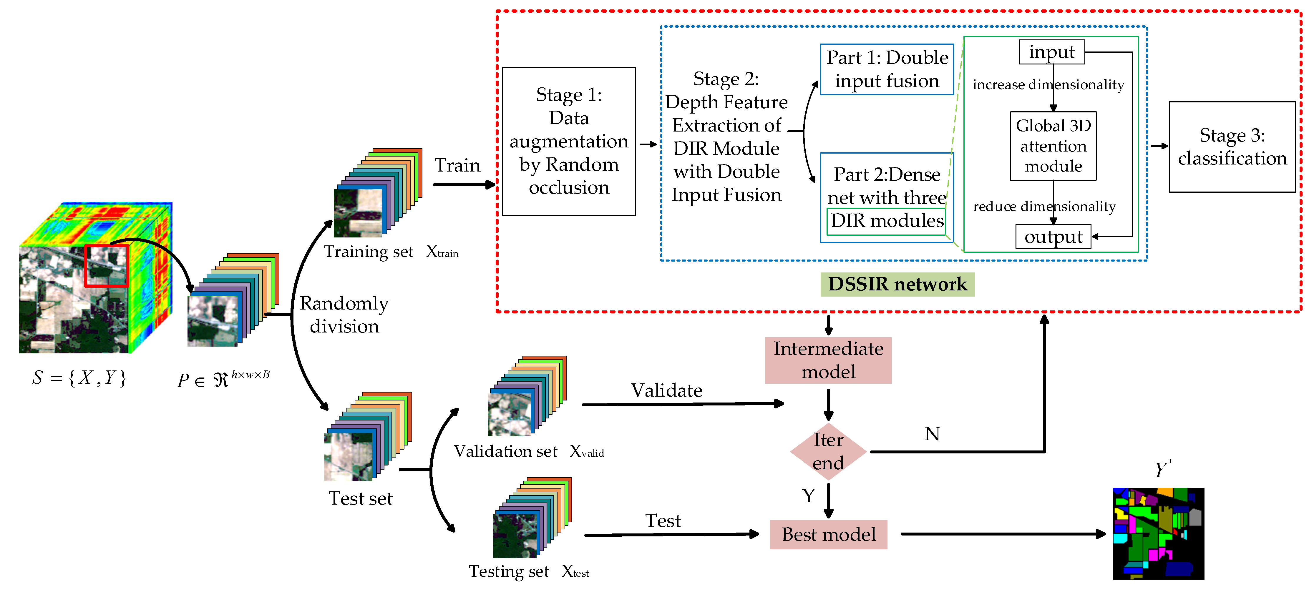
The overall framework of the proposed method is shown in Figure 1. Set $S=\{X,Y\}$ is the input of the model, where $X\in {\Re }^{H\times W\times B}$ is the 3D HSI cube with height $H$, width $W$, and the number of spectral channel $B$, and $Y$ is the label vector of HSI data. Firstly, $X\in {\Re }^{H\times W\times B}$ is randomly divided into some 3D blocks, which are composed of marked central samples and adjacent samples, and are recorded as a new sample set $P\in {\Re }^{h\times w\times B}$, where $h$, $w$, and $B$ represent the height, width, and spectral dimension of the new 3D cube, respectively.

$h$ and $w$ are set to the same value. Then, the training set $X_{train}$ is randomly sampled from the new sample set according to a certain proportion $P$, and then the validation set $X_{valid}$ is randomly sampled from the rest according to the same proportion. Finally, the remaining proportion is used as the test set $X_{test}$. Next, the DSSIRNet is trained with the training set $X_{train}$ to obtain the initial parameters of the model, and the parameters are continuously updated through the validation set $X_{valid}$ until the optimal parameters are obtained. Finally, the test set $X_{test}$ is input into the optimal model to obtain the final prediction results $Y^{\text{'}}$.

2.1. The Overall Framework of the Proposed DSSIRNet

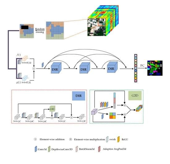
Figure 2 shows the structure of the proposed DSSIRNet. The framework is divided into three stages: data augmentation based on random erasing, deep feature extraction with dual-input fusion and DIR module, and classification. The first stage is designed to solve the problem of limited labeled samples of hyperspectral images. Through block random erasing of training samples, the spatial distribution of the dataset can be fully changed, and the number of available training samples can be effectively increased without parameter increase. In order to improve the robustness of the model, it is necessary to solve the problem of insufficient spectral spatial information extraction of hyperspectral images. The second stage of a deep feature extraction network can solve this problem. The second stage mainly includes two parts: (1) dual-input fusion part; (2) DIR dense connection part. In the second part of this stage, three DIR modules are densely connected to enhance the ability of feature representation. This paper also designs a global 3D attention module in the DIR module to achieve more refined and sufficient global context feature extraction. Finally, the spectral spatial features fully extracted in the second stage are input into the third stage to realize classification.

2.2. Block Random Erasing Strategy for Data Augmentation

In the imaging process, hyperspectral images may be occluded by clouds, shadows or other objects due to the influence of the atmosphere, resulting in the loss of information in the occluded area. The most common interference is cloud cover. Therefore, in the first stage, this paper designs a block random erasing strategy. Before model training, first, the image scene is simulated under cloud erasing conditions, and then the space block with added interference is input into the model for training. It realizes the change of spatial information, increases the available samples, and then improves the classification accuracy. Different from [40], the feature extraction classification model proposed in this paper is three-dimensional. In order to avoid the high complexity of the model, the random erasing under small spatial blocks (i.e., 9 × 9) is studied.

For the training sample set $X_{train}$, $S$ is the spatial area of the original input 3D cube, the erasing probability is set to $p$, the area of the random initialization erasing area is set to $S_e$, the ratio $\frac{S_e}{S}$ is set between $p_l$ and $p_h$, and the ratio $r_e$ of height and width of $S_e$ is set between $r_1$ and $r_2$. First, a probability $p_1=Rand(0,1)$ is randomly obtained. If $p_1<p$ is satisfied, erasure is implemented; otherwise, it will not be processed. In order to obtain the position of the erasing area, first the initial erasing area $S_e=rand(p_l,p_h)\ast S$ is calculated according to the randomly erasing proportion, and then the length and width of the erasing area is calculated according to the random height to width ratio:

$$r_e=rand(r_1,r_2)$$

(1)

$$H_e=\sqrt{S_e\ast r_e}$$

(2)

$$W_e=\sqrt{\frac{S_e}{r_e}}$$

(3)

Then, according to the randomly height and width value, the coordinate $(x_e,y_e)$ of the upper left corner of the erasing area can be obtained. According to the height and width obtained by Formulas (1)–(3), the boundary coordinates of the occluded area $(x_e+W_e,y_e+H_e)$ can be obtained. If the coordinates exceed the boundary of the original space, the above process is repeated. For each iteration of training, random erasing is performed to generate a changing 3D cube, which enables the model to learn more abundant spatial information.

2.3. Dual-Input Fusion Part

Let $x\in X_{train}{}^{h\times h\times l}$ be the data processed by random erasing. After spectral processing $f(\cdot )$ and spatial processing $g(\cdot )$, two groups of feature maps are obtained as the dual input of DIR module. In fact, $f(\cdot )$ and $g(\cdot )$ are the combination functions of three-dimensional convolution, batch normalization (BN), and swish activation functions. The difference between $f(\cdot )$ and $g(\cdot )$ is that the convolution kernel of three-dimensional convolution is different, and the corresponding feature map is

$$M_{spectral}=f\left(x\right)=\sigma (B{N}_{\gamma ,\beta }[(W_1\ast x+b_1)])$$

(4)

$$M_{spatial}=g\left(x\right)=\sigma (B{N}_{\gamma ,\beta }[(W_2\ast x+b_2)])$$

(5)

where $M_{spectral}$ and $M_{spatial}$ are the feature maps obtained by spectral processing and spatial processing, respectively, $\sigma$ represents swish activation function operation, $\ast$ represents three-dimensional convolution operation, $W_i$ and $b_i$ are the weight and bias of two convolution, respectively, and $\gamma$ and $\beta$ represent the trainable parameters of BN operation, respectively. The three-dimensional convolution kernels of spectral processing and spatial processing are $1\times 1\times 9$ and $3\times 3\times 9$, respectively. The number of convolution kernels is 32, the convolution stride is $(1,1,2)$, and the paddings are $(0,0,0)$ and $(1,1,0)$, respectively. Therefore, the size and number of the two groups of feature maps are the same. Then, the obtained two groups of feature maps are directly added and fused element by element, which can be represented as

$$M_{sum}=M_{spectral}\oplus M_{spatial}$$

(6)

where $\oplus$ represents the element by element addition operation, and $M_{sum}$ represents the fused feature map.

2.4. DIR Module

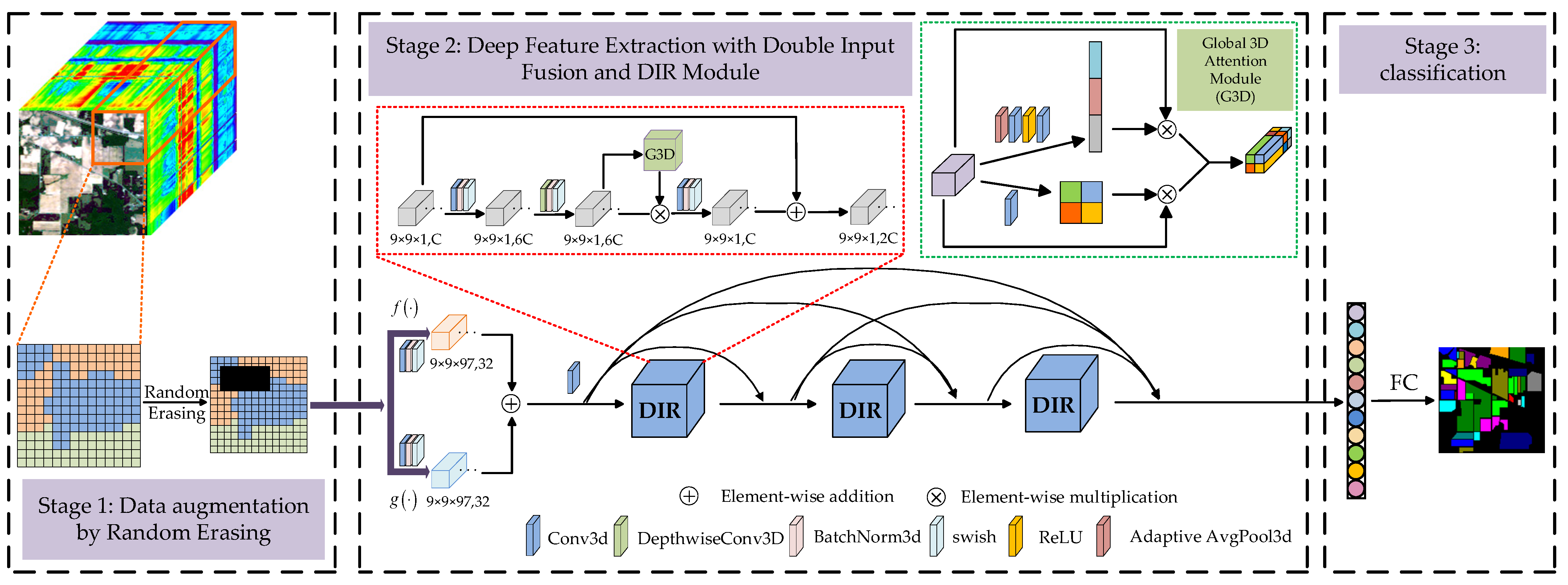
The DIR module designed in this paper is inspired by Mobilenet v3 [42] and Efficientnet [43]. We expand the 2D inverted residual model to 3D inverted residual model. Through a large number of experiments and parameter adjustment, a 3D general module suitable for hyperspectral image classification is designed. Figure 3 shows the schematic diagram of the DIR module.

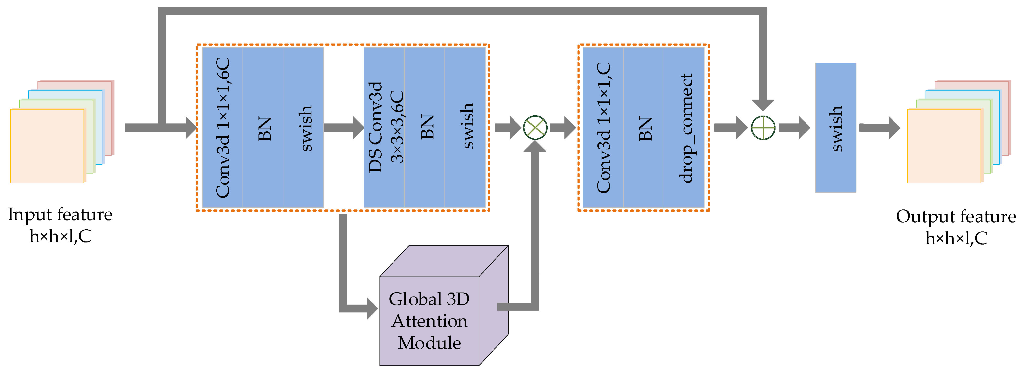
The main idea of deep extraction of spectral spatial features in a DIR module is to expand the low-dimensional representation of input data to high-dimensional representation and filter the feature maps with depthwise separable convolution (DSC). The filtered feature maps are also transmitted to the global 3D attention module for deeper filtering. Following this, the two groups of filtered features are multiplied to enhance feature representation, and then these features are projected back to the low-dimensional representation by standard convolution. Finally, the residual branch is utilized to avoid network degradation. The implementation details of DIR module are described in Algorithm 1.

Algorithm 1 DIR module.

Input: The feature map set $x_l\in {\Re }^{h\times h\times l,C}$ obtained after dual-input fusion.

1: Ascend the dimension of input data $x_l\in {\Re }^{h\times h\times l,C}$ by Conventional 3D convolution. The number of feature maps after convolution is $6C$, and then the feature maps are activated by BN and swish.

2: DSC is performed on the feature maps in two steps: depthwise process and pointwise process. The convolution kernels of the two convolution processes are set to $3\times 3\times 3$ and $1\times 1\times 1$, respectively. The number of feature maps before and after DSC remains the same. Following this, BN and swish activation are performed on these feature maps and then the filtered feature map set $D_{l+1}$ is obtained.

3: Input $D_{l+1}$ into the global 3D attention module for depth filtering and obtain the feature map set $G_{3D}$.

4: Calculate the product of feature maps $\widehat{G_{3D}}=D_{l+1}\otimes G_{3D}$.

5: Reduce the dimension of the multiplied feature map $\widehat{G_{3D}}$ through conventional three-dimensional convolution, and then perform the BN and swish to obtain the reduced feature map set $x_{l+1}\in {\Re }^{h\times h\times l,C}$.

6: Add the input feature map and the reduced dimension feature map, and then activate them with swish to obtain the output feature map set $y_l=\sigma (x_l\oplus x_{l+1})$.

Output: Feature map set $y_l\in {\Re }^{h\times h\times l,C}$ with the same size and number as the input feature map.

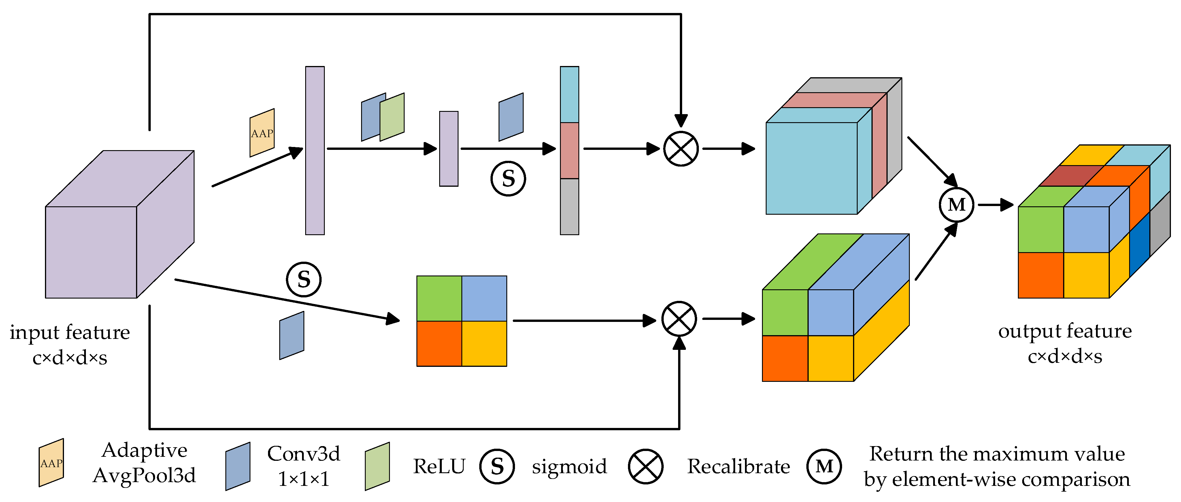
2.5. Global 3D Attention Module

Inspired by csSE [44], this paper designs the global 3D attention module, as shown in Figure 4. The global 3D attention module fully considers the global information and effectively extracts the spectral and spatial context features, so as to enhance the ability of feature representation.

The 3D spectral part: firstly, the input feature map $U=\left[u_1,u_2,\dots ,u_s\right]$ as a combination of spectral channels $u_i\in {\Re }^{d\times d\times s}$, is processed by adaptive average pooling (AAP), and the tensor of element $k$ is obtained:

$$z_k=\frac{1}{d\times d\times s}{\displaystyle \sum _{i=0}^d{\displaystyle \sum _{j=0}^d{\displaystyle \sum _{n=0}^s{U}_k(i,j,n)}}}$$

(7)

Then, two linear layers with size $\frac{c}{2}\times 1\times 1\times 1$ and $c\times 1\times 1\times 1$ are trained to find the correlation between features and classification, and the $s$-dimensional tensor is obtained. Next, the sigmoid function is used for normalization to obtain the spectral attention map. Finally, the obtained spectral attention map is multiplied by the input feature map. The process can be represented as

$$F_c(U)=[\delta (\widehat{z_1})U_1,\delta (\widehat{z_2})U_2,\dots ,\delta (\widehat{z_s})U_s]$$

(8)

where $\delta (\widehat{z_s})$ represents the combination function of two linear layers, ReLU operation and sigmoid activation operation, and $F_c(U)$ is the spectral attention map.

The 3D spatial part: firstly, the image features are extracted through C convolution layers, then the spatial attention map is activated by sigmoid function, and finally the obtained spatial attention map is multiplied by the input feature map. The process can be represented as

$$F_s(U)=[\delta (\widehat{q_1})U_1,\delta (\widehat{q_2})U_2,\dots ,\delta (\widehat{q_s})U_s]$$

(9)

where $\delta (\widehat{q_s})$ is the combination function of one-layer three-dimensional convolution and sigmoid activation operation, and $F_s(U)$ is the spatial attention map.

Finally, the feature maps obtained from the two parts are compared element by element, and the maximum value is returned to generate the final global 3D attention map.

3. Experimental Setting and Results

3.1. Experimental Setting

(1)

Datasets

In order to verify the performance of DSSIRNet, four classical datasets are used in the experiment.

The Indian Pines (IN) dataset was obtained from the airborne visible infrared imaging spectrometer (AVIRIS) sensor in northwestern Indiana. The data size is 145 × 145, a total of 220 continuous imaging bands for ground objects. After excluding 20 bands of 104–108, 150–163, and 200 that cannot be reflected by water, the remaining 200 effective bands are taken as the research object. The spatial resolution is 20 m per pixel and the spectral coverage is 0.4~2.5 μm. There are 16 kinds of crops.

The Pavia University (UP) dataset was collected by ROSIS sensor. It continuously images 115 bands in the wavelength range of 0.43~0.86 μm, with a spatial resolution of 1.3 m. After eliminating the noise influence band, the size of UP is 610 × 340 × 103, including nine types of land cover.

The Salinas Valley (SV) dataset was captured by AVIRIS sensors in Salinas Valley, California. The spatial resolution of the data is 3.7 m, and the size is 512 × 217. The original data is 224 bands. After removing 20 bands of 108–112, 154–167, and 224 with serious water vapor absorption, 204 effective bands are retained. The dataset contains 16 crop categories.

The Botswana (BS) dataset was gathered from the NASA EO-1 satellite over Okavango Delta, Botswana, with a spatial resolution of 30 m and spectral coverage of 0.4~2.5 μm. After excluding the uncalibrated bands covering the water absorption characteristics and noise bands, 145 bands of 10–55, 82–97, 102–119, 134–164, and 187–220 are left for research. The data size is 1476 × 256. The ground truth map can be divided into 14 categories.

In the follow-up experiment, the IN, UP, SV, and BS datasets are divided into training set, validation set, and test set, respectively. The proportion of training, validation, and test randomly selected from each category is the same. The training proportion is equal to the ratio of the number of training samples obtained by random sampling to the total number of samples. The principle of validation proportion and test proportion is similar. Here, in order to avoid missing training samples of some categories in the IN dataset, we randomly select 5% for training, 5% for validation, and the remaining 90% for testing. The proportion of training set, validation set, and test set randomly selected from UP dataset, SV dataset, and BS dataset is the same, which are 3%, 3%, and 94% respectively. The detailed division information of the four datasets is listed in

Table 1. Land cover category and number of samples for training, validation, and testing of IN and UP.

Setting		IN				UP
No	Color	Class	Train	Val	Test	Class	Train	Val	Test
1		Alfalfa	2	2	42	Asphalt	199	199	6233
2		Corn-notill	71	71	1286	Meadows	559	559	17,531
3		Corn-mintill	42	42	746	Gravel	63	63	1973
4		Corn	12	12	213	Trees	92	92	2880
5		Grass-pasture	24	24	435	Painted metal sheets	40	40	1265
6		Grass-trees	36	36	658	Bare Soil	151	151	4727
7		Grass-pasture-mowed	1	1	26	Bitumen	40	40	1250
8		Hay-windrowed	24	24	430	Self-Blocking Bricks	110	110	3462
9		Oats	1	1	18	Shadows	28	28	891
10		Soybean-notill	49	49	874	—	—	—	—
11		Soybean-mintill	123	123	2209	—	—	—	—
12		Soybean-clean	30	30	533	—	—	—	—
13		Wheat	10	10	185	—	—	—	—
14		Woods	63	63	1139	—	—	—	—
15		Building-grass-trees-drives	19	19	348	—	—	—	—
16		Stone-steal-towers	5	5	83	—	—	—	—
Total			512	512	9225	—	1282	1282	40,212

and

Table 2. Land cover category and number of samples for training, validation, and testing of SV and BS.

Setting		SV				BS
No	Color	Class	Train	Val	Test	Class	Train	Val	Test
1		Brocoli-green-weeds-1	60	60	1889	Water	7	7	256
2		Brocoli-green-weeds-2	108	108	3510	Hippo grass	5	5	91
3		Fallow	54	54	1868	Floodplain grasses1	7	7	237
4		Fallow-rough-plow	36	36	1322	Floodplain grasses2	7	7	201
5		Fallow-smooth	78	78	2522	Reeds	7	7	255
6		Stubble	114	114	3731	Riparian	7	7	255
7		Celery	102	102	3375	Fierscar	7	7	245
8		Grapes-untrained	336	336	10,599	Island interior	7	7	189
9		Soil-vineyard-develop	186	186	5831	Acacia woodlands	10	10	294
10		Corn-senesced-green-weeds	96	96	3086	Acacia shrublands	7	7	234
11		Lettuce-romaine-4wk	30	30	1008	Acacia grasslands	10	10	285
12		Lettuce-romaine-5wk	54	54	1819	Short mopane	5	5	171
13		Lettuce-romaine-6wk	24	24	868	Mixed mopane	7	7	254
14		Lettuce-romaine-7wk	30	30	1010	Exposed soils	2	2	91
15		Vineyard-untrained	216	216	6836	—	—	—	—
16		Vineyard-vertical-trellis	54	54	1699	—	—	—	—
Total			1578	1578	50,973	—	95	95	3058

respectively.

(2)

Experimental Setting and Evaluation Index

In the experiment, the batch size of each dataset was set to 16 and the input spatial size was 9 × 9. In this paper, Adam optimizer was adopted. The initial learning rate was set to 0.0003, and the patience value was set to 15 with cosine attenuation. In addition, the maximum training epoch was set to 200. The experimental hardware platform is a server with Intel (R) Core (TM) i9-9900k CPU, NVIDIA GeForce RTX 2080 Ti GPU and 32 G memory. The experimental software platform is based on Windows 10 Visual Studio Code operating system, and adopts CUDA 10.0, Pytorch 1.2.0, and Python 3.7.4. The classification results of all the experiments were the average classification accuracy ± standard deviation through experiments more than 20 times. In order to provide a quantitative evaluation, this paper uses overall accuracy (OA), average accuracy (AA), and kappa coefficient (kappa) as the measures of classification performance. OA represents the ratio of the number of correctly classified samples to the total number of samples. AA indicates the classification accuracy of each category. Kappa coefficient measures the consistency between the results and the real ground map, which is an index to measure the accuracy of classification. Its calculation is based on the confusion matrix. The lower the Kappa value, the more imbalanced the confusion matrix, and the worse the classification effect.

3.2. Classification Results Compared with Other Methods

This paper compares the proposed DSSIRNet with some state-of-the-art classification methods, including SVM_RBF [14], DRCNN [45], ROhsi [40], SSAN [46], SSRN [29], and A²S²K-ResNet [47]. SVM_RBF is a pixel based classification method, DRCNN and ROhsi are 2D-CNN based methods, and SSRN is a method based on RNN and 2D-CNN. The remaining two methods and the proposed DSSIRNet are 3D-CNN based methods.

Table 3. Classification results of different methods on the IN dataset.

Class.	SVM-RBF [14]	DRCNN [45]	ROhsi [40]	SSAN [46]	SSRN [29]	A2S2K-ResNet [47]	DSSIRNet
1	35.17 ± 23.03	95.75 ± 3.41	68.25 ± 4.89	58.26 ± 3.47	97.30 ± 3.52	95.99 ± 6.88	98.88± 1.35
2	62.79 ± 3.24	87.63 ± 4.68	71.01 ± 0.60	65.01 ± 1.98	94.54 ± 3.20	94.88 ± 1.86	96.65± 2.50
3	68.52 ± 3.51	91.40 ± 5.62	79.54 ± 1.34	82.75 ± 13.96	95.13 ± 3.10	94.54 ± 2.04	96.64± 1.22
4	52.79 ± 7.87	88.37 ± 4.10	77.10 ± 5.62	87.10 ± 2.71	96.15 ± 2.02	96.59 ± 2.76	94.81 ± 2.66
5	86.19 ± 3.77	85.87 ± 2.12	85.16 ± 3.29	89.02 ± 2.48	97.67 ± 2.52	98.41 ± 1.10	98.62 ± 1.37
6	85.50 ± 2.78	97.79 ± 3.57	89.05 ± 5.23	96.99 ± 0.68	98.21 ± 0.91	98.38 ± 1.33	99.13± 0.58
7	75.54 ± 10.29	92.26 ± 1.99	71.79 ± 11.02	68.84 ± 16.49	82.07 ± 21.96	85.05 ± 12.34	94.18 ± 5.65
8	89.32 ± 2.00	99.08 ± 2.63	87.78 ± 2.02	98.48 ± 2.92	98.26 ± 3.24	99.75 ± 0.09	99.92± 0.38
9	59.87 ± 20.28	56.75 ± 9.04	40.74 ± 6.92	73.08 ± 36.90	85.91 ± 15.93	72.41 ± 18.63	83.71 ± 18.72
10	68.69 ± 3.36	97.18 ± 2.65	86.69 ± 1.30	93.38 ± 3.11	93.56 ± 2.44	94.72 ± 2.30	97.07 ± 4.77
11	69.97 ± 2.39	92.45 ± 2.78	90.12 ± 0.41	90.39 ± 3.09	97.34 ± 1.01	97.11 ± 1.55	97.65 ± 2.90
12	61.25 ± 5.31	98.03 ± 0.86	86.04 ± 4.54	96.65 ± 1.06	96.85 ± 2.19	95.77 ± 2.22	98.69± 0.92
13	87.18 ± 5.29	99.56 ± 0.18	86.48 ± 5.01	99.05 ± 1.14	99.57 ± 0.84	98.78 ± 1.50	100.0 ± 0.0
14	89.37 ± 1.73	98.23 ± 1.19	96.90 ± 0.28	97.48 ± 1.75	97.54 ± 1.76	97.54 ± 1.41	98.78 ± 1.21
15	69.36 ± 5.32	85.34 ± 0.97	76.50 ± 2.63	96.39 ± 2.75	95.94 ± 3.58.	95.62 ± 2.66	95.76 ± 2.60
16	98.61 ± 2.25	77.04 ± 4.70	81.34 ± 14.16	94.19 ± 7.80	94.17 ± 4.21	92.55 ± 5.62	98.70 ± 1.10
OA (%)	73.74 ± 1.30	94.87 ± 0.92	85.24 ± 0.52	85.79 ± 6.32	96.07 ± 0.73	96.38 ± 0.58	97.18± 0.61
AA (%)	72.50 ± 2.30	90.17 ± 1.59	79.65 ± 1.04	86.71 ± 3.03	95.00 ± 2.38	94.20 ± 1.18	96.82± 3.05
Kappa (%)	69.79 ± 1.49	94.36 ± 1.09	83.12 ± 0.60	83.78 ± 5.51	95.86 ± 0.84	95.88 ± 0.67	96.78± 0.69

,

Table 4. Classification results of different methods on the UP dataset.

Class	SVM-RBF [14]	DRCNN [45]	ROhsi [40]	SSAN [46]	SSRN [29]	A2S2K-ResNet [47]	DSSIRNet
1	88.56 ± 7.71	95.75 ± 0.08	93.63 ± 1.27	94.63 ± 0.21	99.01 ± 0.08	99.44 ± 0.37	99.04 ± 0.53
2	97.12 ± 0.09	94.73 ± 1.20	96.99 ± 0.84	100.0 ± 0.0	98.99 ± 0.20	97.71 ± 3.08	100.0± 0.0
3	81.19 ± 9.07	90.40 ± 3.28	78.44 ± 2.08	76.39 ± 10.09	96.79 ± 1.62	96.11 ± 5.11	98.70± 0.54
4	86.58 ± 7.77	97.37 ± 0.23	96.56 ± 1.16	96.64 ± 0.63	97.98 ± 1.03	99.59 ± 0.18	97.98 ± 0.52
5	98.39 ± 0.08	98.87 ± 0.05	97.49 ± 1.75	97.84 ± 0.74	100.0 ± 0.0	100.0 ± 0.0	100.0 ± 0.0
6	85.63 ± 1.89	95.70 ± 1.34	91.05 ± 0.69	87.90 ± 9.81	99.31 ± 0.55	100.0 ± 0.0	100.0 ± 0.0
7	85.81 ± 3.95	89.06 ± 11.37	84.30 ± 5.07	89.54 ± 8.05	99.69 ± 0.45	99.24 ± 1.01	99.39 ± 0.63
8	83.92 ± 0.98	96.19 ± 0.93	97.73 ± 0.47	92.99 ± 4.67	82.82 ± 1.81	95.95 ± 1.02	97.86 ± 0.51
9	99.12 ± 0.62	96.60 ± 1.32	99.36 ± 0.43	98.55 ± 0.06	99.86 ± 0.21	99.69 ± 0.28	99.89 ± 0.08
OA (%)	91.49 ± 1.04	95.79 ± 0.97	94.57 ± 0.51	94.35 ± 3.31	97.62 ± 0.71	98.22 ± 1.71	99.31 ± 0.06
AA (%)	89.59 ± 5.69	94.96 ± 0.51	92.84 ± 0.81	92.72 ± 1.28	97.16 ± 0.36	98.63 ± 0.99	99.20 ± 0.15
Kappa (%)	88.68 ± 3.08	94.67 ± 0.29	92.80 ± 0.67	92.44 ± 3.09	96.83 ± 1.42	97.62 ± 2.29	99.05 ± 0.08

,

Table 5. Classification results of different methods on the SV dataset.

Class	SVM-RBF [14]	DRCNN [45]	ROhsi [40]	SSAN [46]	SSRN [29]	A2S2K-ResNet [47]	DSSIRNet
1	99.13 ± 0.31	98.84 ± 0.17	99.96 ± 0.04	99.66 ± 0.15	99.92 ± 0.09	100.0 ± 0.0	100.0± 0.0
2	99.22 ± 0.40	99.61 ± 0.09	99.96 ± 0.05	99.94 ± 0.02	100.0 ± 0.0	100.0 ± 0.0	100.0± 0.0
3	99.05 ± 1.70	99.75 ± 0.06	95.80 ± 1.79	96.62 ± 2.16	99.82 ± 0.25	99.74 ± 0.25	99.86± 0.13
4	98.67 ± 0.35	98.79 ± 0.35	99.11 ± 1.25	98.91 ± 0.62	98.90 ± 0.75	99.46 ± 0.40	99.66 ± 0.68
5	97.81 ± 0.19	98.84 ± 1.01	98.62 ± 0.73	99.79 ± 0.04	99.78 ± 0.29	99.58 ± 0.51	99.91 ± 0.82
6	98.62 ± 1.62	99.07 ± 0.80	98.27 ± 0.60	98.17 ± 0.43	99.98 ± 0.02	100.0 ± 0.0	100.0± 0.0
7	99.62 ± 2.02	89.05 ± 9.25	99.80 ± 0.22	99.79 ± 0.28	99.89 ± 0.15	100.0 ± 0.0	100.0 ± 0.0
8	81.91 ± 16.99	97.17 ± 2.23	88.66 ± 1.39	82.53 ± 9.37	99.55 ± 0.17	98.88 ± 0.87	99.07 ± 0.63
9	99.08 ± 0.85	96.88 ± 3.60	98.79 ± 0.20	100.0 ± 0.0	98.91 ± 0.14	99.93 ± 0.08	100.0± 0.0
10	88.26 ± 4.86	89.34 ± 0.41	97.29 ± 0.76	99.25 ± 0.53	98.68 ± 0.75	99.48 ± 0.32	99.79± 0.12
11	91.98 ± 4.17	100.0 ± 0.0	97.18 ± 0.73	99.53 ± 0.17	87.89 ± 14.41	98.59 ± 1.98	97.78 ± 3.00
12	99.14 ± 0.79	95.43 ± 1.37	97.94 ± 1.02	98.72 ± 1.15	99.74 ± 0.20	99.09 ± 1.16	100.0± 0.0
13	98.42 ± 2.43	98.97 ± 0.48	96.90 ± 0.39	96.20 ± 2.97	94.57 ± 7.67	98.50 ± 1.95	99.80± 0.11
14	91.49 ± 5.85	82.24 ± 11.34	97.48 ± 0.48	98.45 ± 0.93	98.99 ± 0.87	99.21 ± 0.51	98.93 ± 1.15
15	71.44 ± 19.45	97.57 ± 1.77	84.76 ± 1.49	90.36 ± 5.02	85.29 ± 5.44	94.06 ± 2.51	98.83± 0.92
16	97.21 ± 2.74	92.72 ± 0.05	88.33 ± 1.87	97.09 ± 1.28	99.93 ± 0.09	99.74 ± 0.18	100.0± 0.0
OA (%)	90.74 ± 0.96	96.63 ± 2.41	94.28 ± 0.16	94.64 ± 4.13	96.80 ± 1.84	98.36 ± 0.56	99.35± 0.09
AA (%)	94.44 ± 0.24	95.89 ± 0.50	96.18 ± 0.07	97.18 ± 2.69	97.62 ± 1.88	99.14 ± 0.55	99.60± 0.22
Kappa (%)	89.68 ± 1.27	94.07 ± 1.83	93.63 ± 0.18	94.02 ± 5.26	96.45 ± 2.05	98.18 ± 0.62	99.27± 0.10

and

Table 6. Classification results of different methods on the BS dataset.

Class	SVM-RBF [14]	DRCNN [45]	ROhsi [40]	SSAN [46]	SSRN [29]	A2S2K-ResNet [47]	DSSIRNet
1	90.94 ± 0.76	84.75 ± 7.20	98.16 ± 0.80	91.13 ± 9.24	98.74 ± 1.35	92.06 ± 3.74	99.96 ± 0.12
2	45.45 ± 31.12	61.00 ± 24.79	68.77 ± 7.56	93.03 ± 4.82	97.47 ± 5.04	100.0 ± 0.0	98.60 ± 1.74
3	94.21 ± 4.87	94.49 ± 0.31	65.81 ± 2.35	87.05 ± 8.24	99.91 ± 0.16	87.45 ± 11.10	100.0 ± 0.0
4	75.12 ± 16.17	82.55 ± 9.35	24.09 ± 9.61	92.99 ± 5.89	96.37 ± 2.96	91.41 ± 1.83	95.74 ± 2.90
5	77.99 ± 9.78	65.47 ± 18.90	52.17 ± 10.31	88.89 ± 10.02	91.05 ± 4.40	82.84 ± 9.50	93.48 ± 3.88
6	65.25 ± 9.65	75.40 ± 11.26	49.14 ± 8.59	50.33 ± 20.13	95.43 ± 4.54	88.66 ± 1.86	96.20 ± 2.97
7	95.65 ± 1.74	99.06 ± 0.03	73.38 ± 3.12	100.0 ± 0.0	100.0 ± 0.0	99.18 ± 0.88	100.0 ± 0.0
8	75.38 ± 16.84	84.20 ± 10.22	54.27 ± 11.85	87.28 ± 5.22	98.37 ± 1.48	97.89 ± 0.70	100.0 ± 0.0
9	81.04 ± 7.52	86.44 ± 7.23	70.27 ± 6.01	71.65 ± 25.43	93.94 ± 4.49	89.98 ± 5.69	99.40 ± 1.18
10	97.01 ± 1.47	87.18 ± 3.05	96.70 ± 3.14	80.24 ± 9.14	99.40 ± 0.42	92.19 ± 3.97	95.41 ± 4.21
11	85.08 ± 7.46	89.70 ± 1.69	83.50 ± 1.99	86.12 ± 7.07	99.82 ± 0.14	96.76 ± 3.64	99.83 ± 1.10
12	58.10 ± 25.59	93.45 ± 3.47	53.60 ± 26.50	67.31 ± 18.24	98.99 ± 0.06	97.00 ± 2.13	99.08 ± 1.54
13	71.65 ± 7.51	77.06 ± 21.13	57.01 ± 4.27	87.07 ± 6.81	99.52 ± 0.94	89.25 ± 7.76	100.0 ± 0.0
14	58.24 ± 7.58	96.95 ± 0.05	98.87 ± 1.58	92.66 ± 5.06	100.0 ± 0.0	100.0 ± 0.0	100.0 ± 0.0
OA (%)	78.80 ± 2.41	86.56 ± 5.77	67.21 ± 4.47	84.17 ± 5.60	97.75 ± 0.44	91.56 ± 0.73	98.14 ± 0.81
AA (%)	76.50 ± 1.92	84.12 ± 4.01	67.55 ± 4.82	83.98 ± 9.54	97.78 ± 0.13	93.19 ± 0.62	98.40 ± 0.67
Kappa (%)	76.98 ± 3.08	84.57 ± 5.18	64.46 ± 4.86	82.87 ± 8.06	97.32 ± 0.47	90.84 ± 0.79	97.96 ± 0.88

list the average classification accuracy of the seven methods on the four datasets. The 2–17 lines record the classification accuracy of specific categories, and the last three lines record OA, AA, and kappa of all categories. In addition, for these experimental results, the best results are highlighted in bold.

As can be seen from Table 3, the classification results of the proposed DSSIRNet method on the IN dataset are obviously superior to those of other state-of-the-art methods, and the best OA, AA, and kappa values are achieved. Because the frameworks based on deep learning (including DRCNN, ROhsi, SSAN, SSRN, A²S²K-ResNet, and DSSIRNet) have excellent nonlinear representation and automatic hierarchical feature extraction capabilities, their classification performances are better than that of SVM_RBF. For the model based on 2D-CNN, the model structures of ROhsi and SSAN are too simple, and the extraction of spectral spatial feature is not sufficient. Therefore, the OAs of the above two methods are 9.63% and 9.08% lower than those of DRCNN, respectively. For the 3D-CNN model, the learning of spectral spatial features of SSRN is separated, and the learned advanced features are not fused. Thus, the OAs of SSRN are lower than that of A²S²K-ResNet and the proposed DSSIRNet method. The proposed DSSIRNet method firstly performed block data augmentation on the input 3D cube to increase the available samples, and then the designed DIR module fully extracted the spectral spatial features. The global 3D attention module also effectively realized the selection and extraction of global context information. The final dense connection operation effectively integrated the joint spectral spatial features learned by the DIR module. Therefore, the OA value of the proposed method on the IN dataset is 0.8% higher than that of A²S²K-ResNet. In particular, the proposed DSSIRNet method also provides a 100% prediction rate for the wheat category.

For the UP dataset and SV dataset, as shown in Table 4 and Table 5, the classification results of all methods exceed 90%. The DRCNN uses multiple input spatial windows, so the OA values are higher than that of SVM_RBF, ROhsi, and SSAN. A²S²K-ResNet can adaptively select 3D convolution kernel to jointly extract spectral spatial features, so its OA values are higher than that of SSRN. Compared with these methods, the OA values obtained by DSSIRNet on the UP dataset are 7.82%, 3.52%, 4.74%, 4.96%, 1.69%, and 1.09% higher than that of SVM-RBF, DRCNN, ROhsi, SSAN, SSRN, and A²S²K-ResNet, respectively. The OA values obtained on the SV dataset are 8.61%, 2.72%, 5.07%, 4.71%, 2.55%, and 0.99% higher than that of SVM-RBF, DRCNN, ROhsi, SSAN, SSRN, and A²S²K-ResNet, respectively. In particular, the proposed DSSIRNet method achieved 100% prediction rate in the three categories of grassland, painted metal plate, and bare soil of UP dataset; on the SV dataset, seven categories achieved 100% prediction rate.

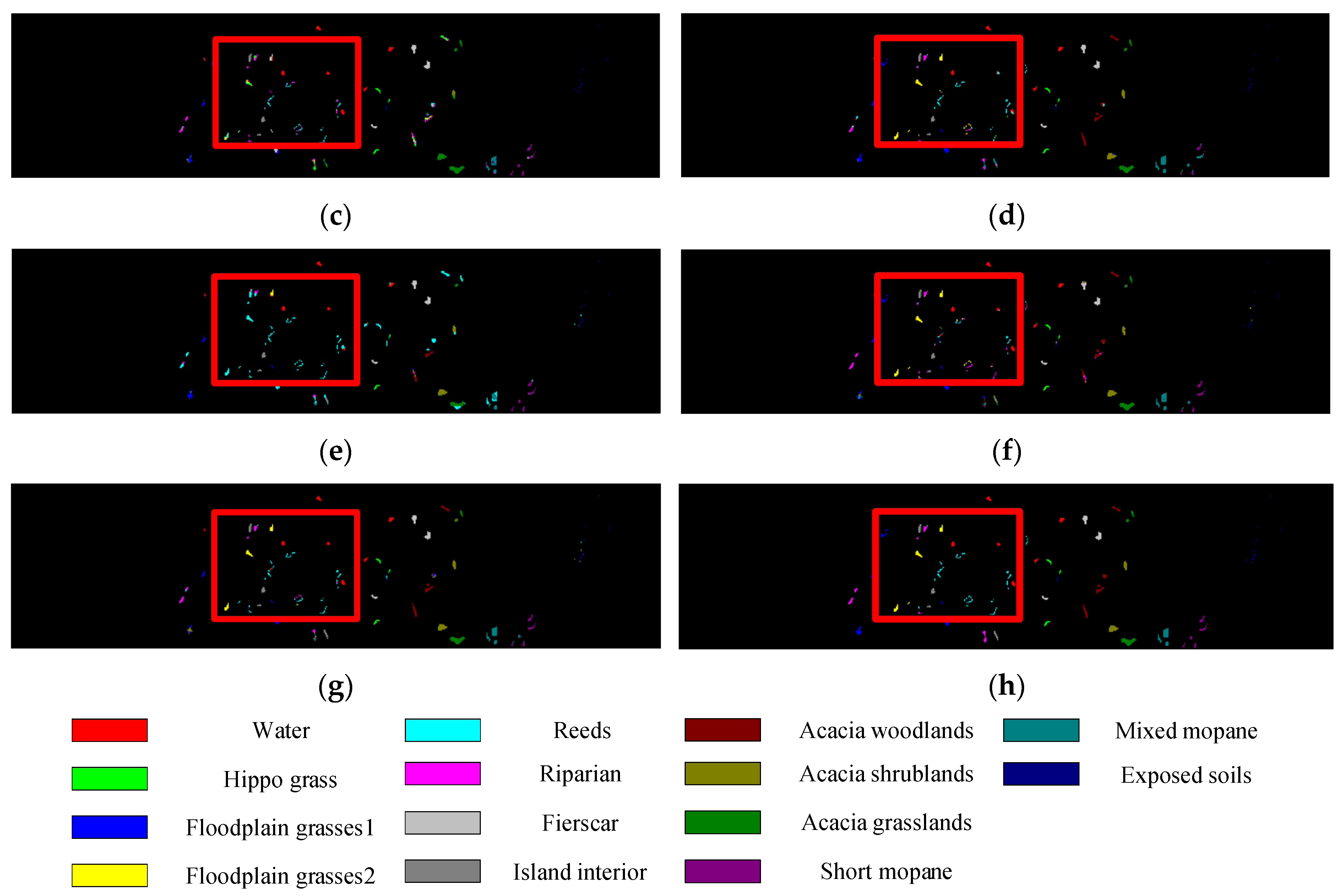
Table 6 shows the classification results of different methods on the BS dataset. Compared with the other three datasets, the BS dataset has the highest spatial resolution, so the classification model is very important for the effective extraction of spatial context information. Obviously, the classification performances based on 3D-CNN (SSRN, A²S²K-ResNet, and DSSIRNet) are higher than other methods, because 3D-CNN can extract spectral and spatial features at the same time. A²S²K-ResNet extracts joint spectral spatial features directly, which may lose spatial context information, so its OA values are lower than that of SSRN. The proposed DSSIRNet method utilized the DIR module to realize the joint extraction of spectral spatial features, and combined the global 3D attention module to focus on the spectral and spatial context features that contribute greatly to the classification, so it achieved the best classification performance.

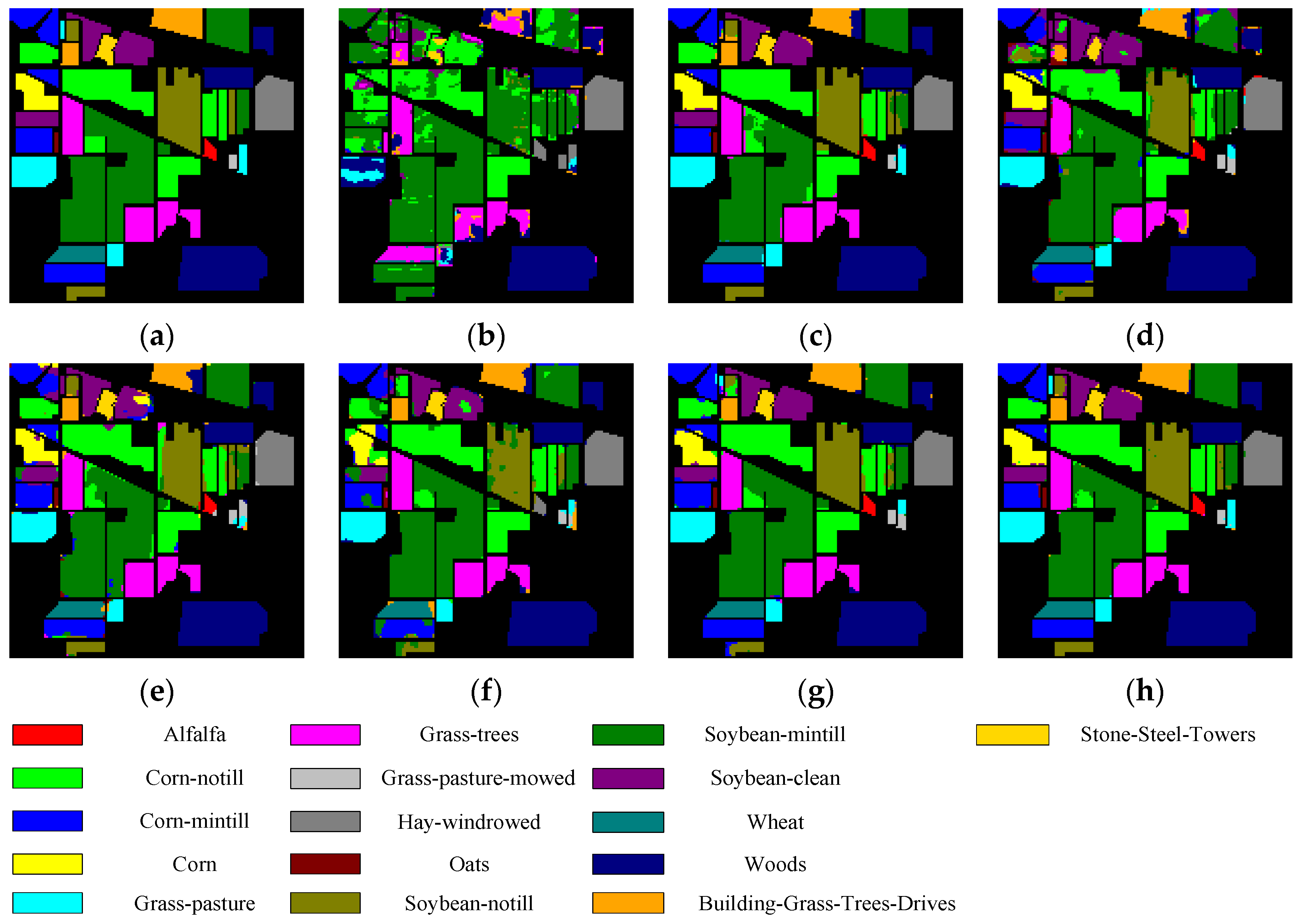
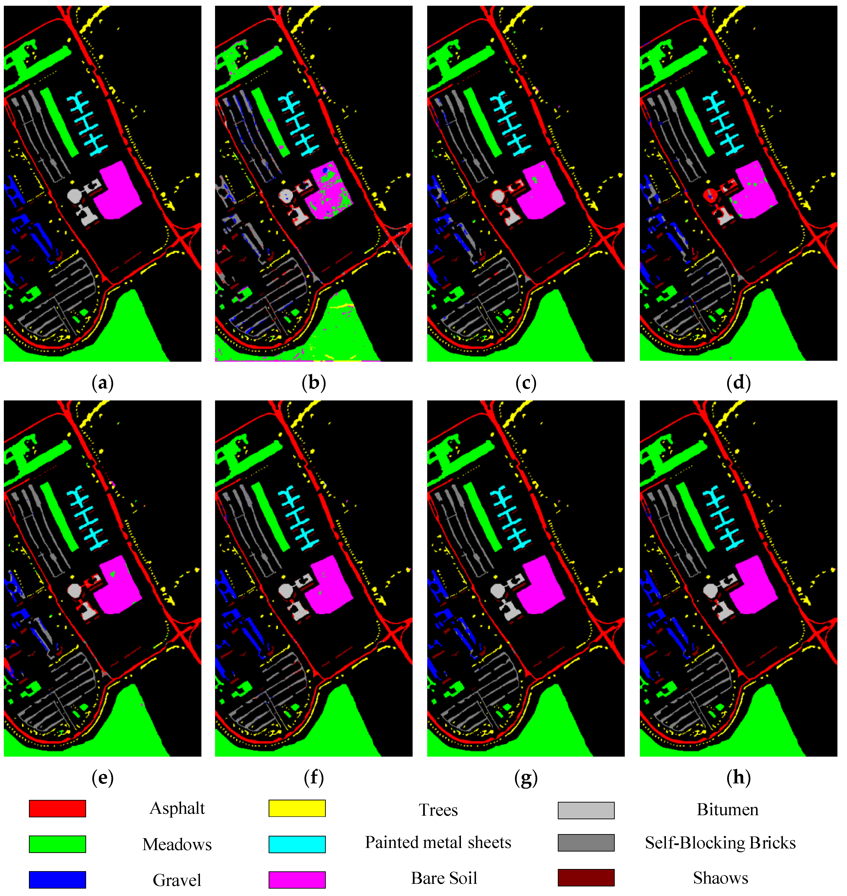
Figure 5, Figure 6, Figure 7 and Figure 8 show the visual classification results obtained by seven methods on four datasets. Taking Figure 5 as an example, the classification maps obtained by SVM_RBF, DRCNN, ROhsi, and SSAN have some noise, especially in the corn-notill, grass-pasture, oats, and soybean-mintill classes. The 3DCNN-based methods (including SSRN, A2S2KResNet and DSSIRNet) extract the spectral spatial features more effectively. Compared with other methods, DSSIRNet greatly improves the regional consistency and make some categories more separable, such as grass-trees, hay-windrowed, and wheat. As can be seen, the probability of misclassification among the categories of SVM_RBF, DRCNN, ROhsi, and SSAN is large, and the misclassification rate among other methods is small. In particular, the proposed DSSIRNet method has the smallest misclassification rate and a clear category boundary, which is closest to the ground real map, which shows the effectiveness of the proposed DSSIRNet method.

4. Experimental Analysis

4.1. Parameter Analysis of Erasing Probability

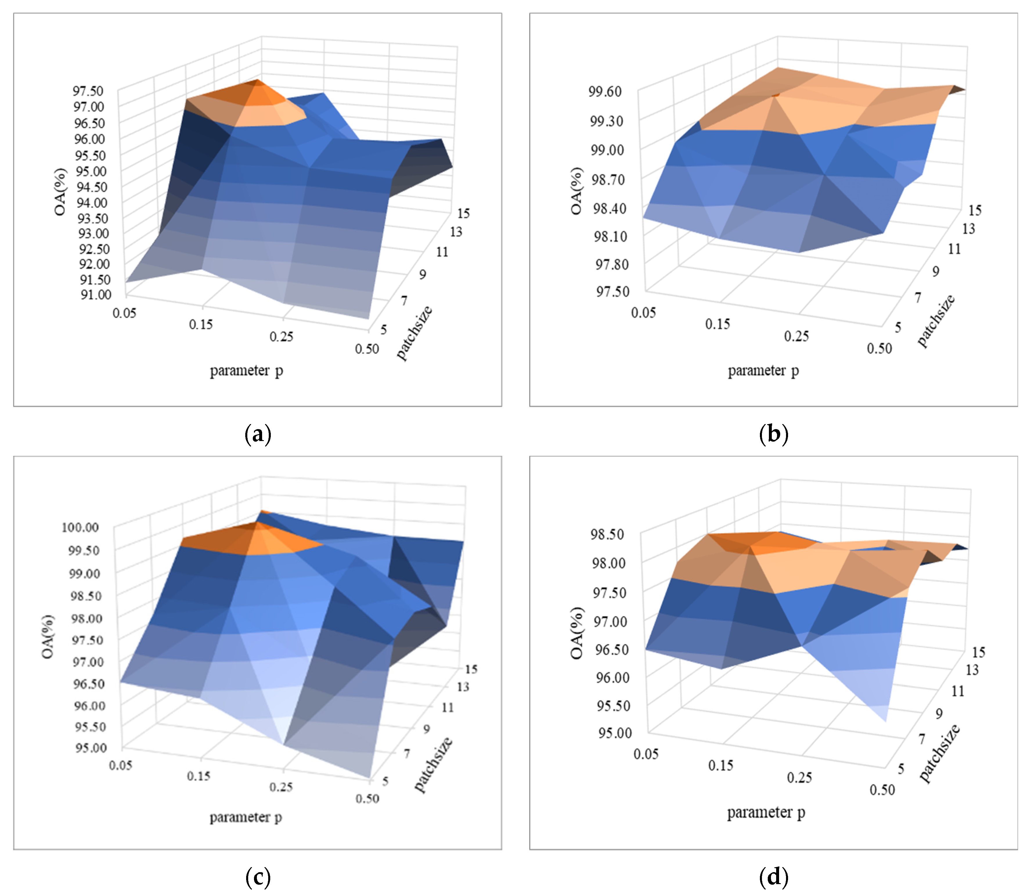
In order to verify the efficiency of random erasing strategy under small spatial blocks, we studied the influence of erasing probability and spatial blocks smaller than 20 × 20 on the classification performance, and showed the comparison results with the surface graph, as shown in Figure 9a–d. It can be seen from Figure 9 that under the same patch size, the OA value reaches the highest value at $p=0.15$, and then the OA values of each dataset begin to decrease with the increase of $p$. From the perspective of patch, for the same parameter $p$, with the increase of patch size, the OA value obtains the highest value of each dataset when the patch size is 9. To sum up, for these hyperspectral datasets, appropriate size of image block (i.e., 9 × 9) and erasing probability (i.e., 0.15) are taken, which not only reduces the computational complexity, but also improves the classification accuracy.

4.2. Run Time Comparison

In addition to classification accuracy, running time is also an important indicator in HSI classification tasks, especially in practical applications.

Table 7. Running time of seven methods on four datasets (s).

	Method	SVM_RBF	DRCNN	ROhsi	SSRN	SSAN	A2S2K-ResNet	DSSIRNet
Dataset
IN		4.7	102.8	83.88	31.7	5.8	39.5	39.6
UP		24.3	142.3	175.5	57.7	23.6	118.5	100.1
SV		55.5	272.7	310.2	120.9	61.1	141.4	219.3
BS		2.5	19.3	27.5	6.9	4.8	10.7	12.7

shows the running time of all methods on four datasets. Compared with other methods based on deep learning, SVM_RBF takes the least time. Because DRCNN uses multiple input space windows for learning, the running time of this method is long. ROhsi sends large space blocks to input 2D-CNN model for training, so the running time is longer than DRCNN. For SSAN, it uses RNN and 2D-CNN to learn spectral spatial features at the same time, where running time is only longer than SVM_RBF. For 3D-CNN models, i.e., SSRN, A²S²K-ResNet, and DSSIRNet, although the proposed DSSIRNet costs slightly more time on SV and BS datasets due to a large number of layers, the running time of it is less than that of DRCNN and ROhsi methods. Therefore, DSSIRNet has moderate computational complexity and can be used in practical applications.

4.3. Efficiency Analysis of Dense Connection of DIR Module

In this section, the efficiencies of the number of DIR modules on four datasets are analyzed, as shown in

Table 8. Number of DIR modules on four datasets (OA%).

Datasets	2 Blocks	3 Blocks	4 Blocks
IN	96.29	97.18	93.91
UP	98.86	99.31	98.99
SV	96.98	99.35	98.85
BS	97.93	98.14	97.85

. As a general module, the DIR module is densely connected, and the joint spectral spatial features extracted by the module can be used most effectively. Firstly, the two DIR blocks are densely connected, and the classification accuracy exceeds that of other methods except 3D-CNN model. When using three DIR modules, the proposed DSSIRNet method achieves the highest classification accuracy. On this basis, after adding another module, the OA value of each dataset decreases significantly. Meanwhile, the number of layers and complexity of the model increase rapidly, which will affect the effective utilization of features. In conclusion, when three DIR modules are adopted, the feature extraction is the most effective and the ability to distinguish features is the strongest.

4.4. Ablation Experiment

In order to verify the performance of the random erasing (RE) strategy and the global 3D attention (G3D) module proposed in this paper, the ablation results of the two modules (strategies) on four datasets are shown in

Table 9. Ablation experiments with different modules or strategies (OA%).

Approach		Datasets
Use RE?	Use G3D?	IN	UP	SV	BS
no	no	95.77	98.56	96.31	97.33
no	yes	95.86	98.94	96.90	98.04
yes	no	96.21	98.89	97.75	98.10
yes	yes	97.18	99.31	99.35	98.14

. It can be seen that when the RE strategy and G3D module are not adopted, the classification accuracy of the four datasets is the lowest. Adding any of these methods will increase the OA value. Because the RE strategy increases the number of available samples, it will have a greater impact on the final classification performance than adding only G3D modules. Obviously, the optimal OA value is obtained by adding both the two methods at the same time (i.e., the proposed DSSIRNet), which can not only realize data augmentation, but also consider the spectral spatial global context information.

4.5. Small Sample Comparative Analysis

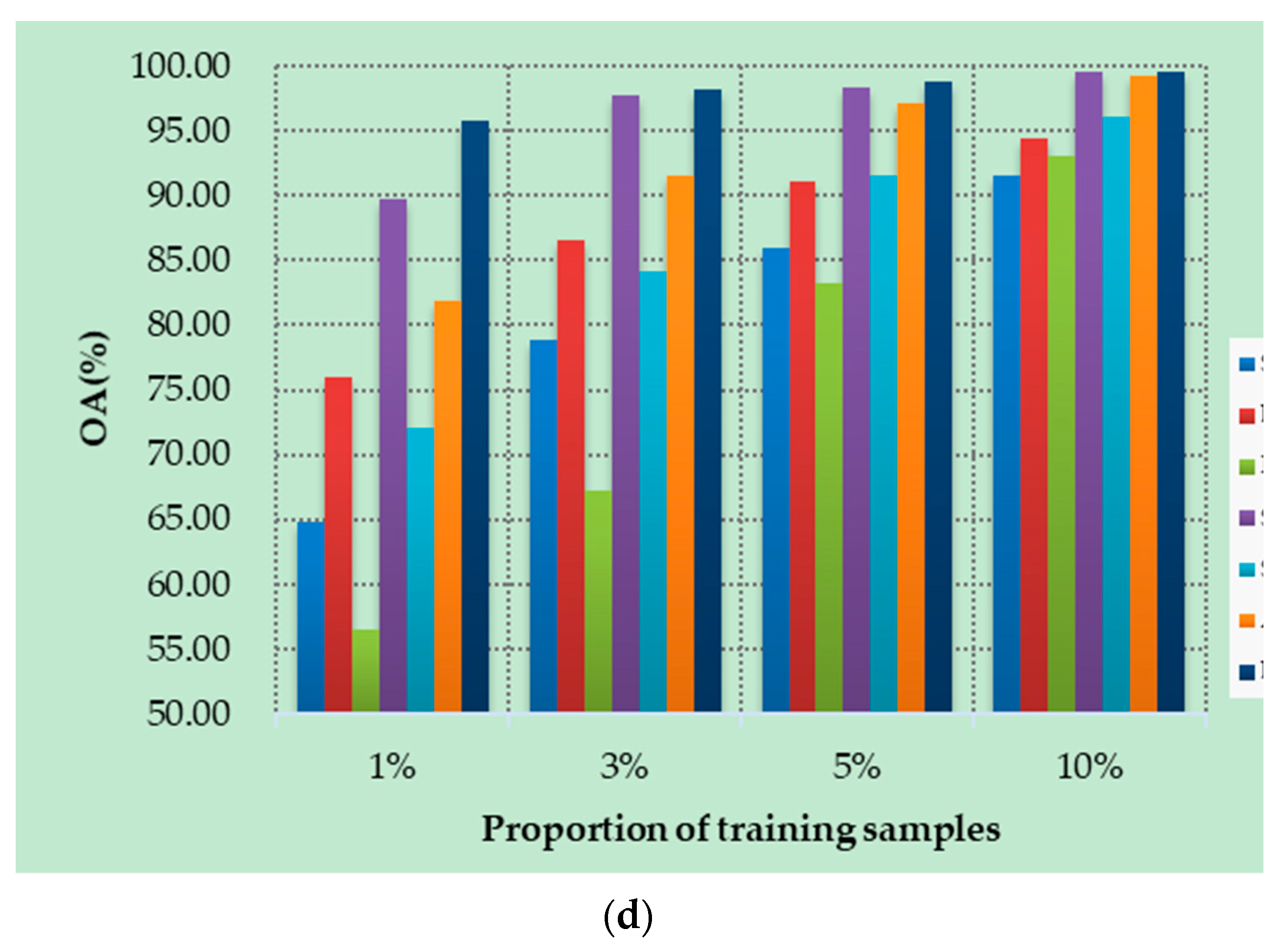
Figure 10a–d show the OAs of all methods on different datasets with different numbers of training samples. Specifically, four datasets are randomly selected from labeled samples, with 1%, 3%, 5%, and 10% training samples in each class. As can be seen from Figure 10, the proposed DSSIRNet method achieves the highest classification accuracy on all four datasets. With the increase of training proportion, the OA values of all methods are improved, and the performance differences between different models are reduced, but the OA value of the proposed method is still the highest. At 1% training samples, compared with other models based on deep learning, ROhsi and SVM_RBF have no advantages. In 5% of the training samples, the OA value of ROhsi on UP and SV increased rapidly, exceeding that of SVM_RBF. Compared with other methods, the proposed DSSIRNet shows the best classification performance in the case of small samples. The reason is that it adopts an effective data augmentation strategy and the DIR module to realize effective feature extraction, which also proves that DSSIRNet has more advantages in the case of small datasets.

5. Conclusions

In this paper, we propose a novel HSI classification network, DSSIRNet. DSSIRNet is divided into three stages. The first stage adopts a random erasing strategy for augmentation of the data of the original 3D cube. The two components of the second stage realize effective joint spectral spatial feature extraction. The third stage classifies high-level semantic features. The full combination of the three stages realizes the optimal classification effect of HSI. In addition, this paper studies the random erasing strategy in small spatial blocks, which can expand the data more effectively without adding parameters. In DSSIRNet, an effective feature extraction module, the DIR module, is designed to fully extract image features. This paper also designs a global 3D attention module to fully consider the global context information of spectral and spatial dimension and further improve the classification performance. The experimental results on four datasets prove the effectiveness of DSSIRNet. In the future, we will study a deep learning framework for HSI classification tasks with low parameters and small samples.

References

- Zhang, X.; Sun, Y.; Shang, K.; Zhang, L.; Wang, S. Crop classification based on feature band set construction and object-oriented approach using hyperspectral images. IEEE J. Sel. Top. Appl. Earth Observ. Remote Sens. 2016, 9, 4117–4128. [Google Scholar] [CrossRef]
- Caporaso, N.; Whitworth, M.B.; Grebby, S.; Fisk, I.D. Non-destructive analysis of sucrose, caffeine and trigonal line on single green coffee beans by hyperspectral imaging. Food Res. Int. 2018, 106, 193–203. [Google Scholar] [CrossRef] [PubMed]
- Tan, H.F.; Luo, T.W.; Yang, G.; Meng, Q.Q. Research on background depression in hyperspectral image anomaly detection. J. Optoelectron. Laser 2016, 27, 177–181. [Google Scholar]
- Yokoya, N.; Chan, J.C.-W.; Segl, K. Potential of resolution enhanced hyperspectral data for mineral mapping using simulated EnMAP and Sentinel-2 images. Remote Sens. 2016, 8, 172. [Google Scholar] [CrossRef] [Green Version]
- Honkavaara, E.; Eskelinen, M.A.; Polonen, I.; Saari, H.; Ojanen, H.; Mannila, R.; Holmlund, C.; Hakala, T.; Litkey, P.; Rosnell, T.; et al. Remote sensing of 3-d geometry and surface moisture of a peat production area using hyperspectral frame cameras in visible to short-wave infrared spectral ranges onboard a small unmanned airborne vehicle (UAV). IEEE Trans. Geosci. Remote Sens. 2016, 54, 5440–5454. [Google Scholar] [CrossRef] [Green Version]
- Zhang, X.; Wang, Y.; Zhang, N.; Xu, D.; Luo, H.; Chen, B.; Ben, G. Spectral-Spatial Fractal Residual Convolutional Neural Network with Data Balance Augmentation for Hyperspectral Classification. IEEE Trans. Geosci. Remote Sens. 2021, 1–15, early access. [Google Scholar] [CrossRef]
- Ahmad, M.; Shabbir, S.; Roy, S.K.; Hong, D.; Wu, X.; Yao, J.; Khan, A.M.; Mazzara, M.; Distefano, S.; Chanussot, J. Hyperspectral Image Classification—Traditional to Deep Models: A Survey for Future Prospects. arXiv 2021, arXiv:2101.06116. [Google Scholar]
- Huang, L.; Chen, C.; Li, W.; Du, Q. Remote sensing image scene classification using multi-scale completed local binary patterns and fisher vectors. Remote Sens. 2016, 8, 483. [Google Scholar] [CrossRef] [Green Version]
- Dalal, N.; Triggs, B. Histograms of oriented gradients for human detection. In Proceedings of the IEEE Computer Society Conference on Computer Visionand Pattern Recognition (CVPR), San Diego, CA, USA, 20–25 June 2005; pp. 886–893. [Google Scholar]
- Oliva, A.; Torralba, A. Modeling the shape of the scene: A holistic representation of the spatial envelope. Int. J. Comput. Vis. 2001, 42, 145–175. [Google Scholar] [CrossRef]
- Ham, J.; Chen, Y.; Crawford, M.M.; Ghosh, J. Investigation of the random forest framework for classification of hyperspectral data. IEEE Trans. Geosci. Remote Sens. 2005, 43, 492–501. [Google Scholar] [CrossRef] [Green Version]
- Li, J.; Bioucas-Dias, J.; Plaza, A. Semisupervised hyperspectral image segmentation using multinomial logistic regression with active learning. IEEE Trans. Geosci. Remote Sens. 2010, 48, 4085–4098. [Google Scholar] [CrossRef] [Green Version]
- Li, W.; Chen, C.; Su, H.; Du, Q. Local binary patterns and extreme learning machine for hyperspectral imagery classification. IEEE Trans. Geosci. Remote Sens. 2015, 53, 3681–3693. [Google Scholar] [CrossRef]
- Melgani, F.; Bruzzone, L. Classification of hyperspectral remote sensing images with support vector machines. IEEE Trans. Geosci. Remote Sens. 2004, 42, 1778–1790. [Google Scholar] [CrossRef] [Green Version]
- Li, S.; Song, W.; Fang, L.; Chen, Y.; Ghamisi, P.; Benediktsson, J.A. Deep learning for hyperspectral image classifification: An overview. IEEE Trans. Geosci. Remote Sens. 2019, 57, 6690–6709. [Google Scholar] [CrossRef] [Green Version]
- Vincent, P.; Larochelle, H.; Lajoie, I.; Bengio, Y.; Manzagol, P.-A. Stacked denoising autoencoders: Learning useful representations in a deep network with a local denoising criterion. J. Mach. Learn. Res. 2010, 11, 3371–3408. [Google Scholar]
- Ng, A. Sparse Autoencoder; Lecture Notes CS294A; Stanford University: Stanford, CA, USA, 2011; pp. 1–19. [Google Scholar]
- Tao, C.; Pan, H.; Li, Y.; Zou, Z. Unsupervised spectral-spatial feature learning with stacked sparse autoencoder for hyperspectral imagery classification. IEEE Geosci. Remote Sens. Lett. 2015, 12, 2438–2442. [Google Scholar]
- Zhang, X.; Liang, Y.; Li, C.; Huyan, N.; Jiao, L.; Zhou, H. Recursive autoencoders-based unsupervised feature learning for hyperspectral image classification. IEEE Geosci. Remote Sens. Lett. 2017, 14, 1928–1932. [Google Scholar] [CrossRef] [Green Version]
- Mou, L.; Ghamisi, P.; Zhu, X. Unsupervised spectral-spatial feature learning via deep residual conv-deconv network for hyperspectral image classification. IEEE Trans. Geosci. Remote Sens. 2018, 56, 391–406. [Google Scholar] [CrossRef] [Green Version]
- Radford, A.; Metz, L.; Chintala, S. Unsupervised representation learning with deep convolutional generative adversarial networks. arXiv 2016, arXiv:1511.06434v2. [Google Scholar]
- Zhu, L.; Chen, Y.; Ghamisi, P.; Benediktsson, J.A. Generative adversarial networks for hyperspectral image classification. IEEE Trans. Geosci. Remote Sens. 2018, 56, 5046–5063. [Google Scholar] [CrossRef]
- Mou, L.; Ghamisi, P.; Zhu, X.X. Deep recurrent neural networks for hyperspectral image classification. IEEE Trans. Geosci. Remote Sens. 2017, 55, 3639–3655. [Google Scholar] [CrossRef] [Green Version]
- Zhang, H.; Li, Y.; Zhang, Y.; Shen, Q. Spectral-spatial classification of hyperspectral imagery using a dual-channel convolutional neural network. Remote Sens. Lett. 2017, 8, 438–447. [Google Scholar] [CrossRef] [Green Version]
- Hao, S.; Wang, W.; Ye, Y.; Nie, T.; Bruzzone, L. Two-stream deep architecture for hyperspectral image classification. IEEE Trans. Geosci. Remote Sens. 2018, 56, 2349–2361. [Google Scholar] [CrossRef]
- Feng, J.; Chen, J.; Liu, L.; Cao, X.; Zhang, X.; Jiao, L.; Yu, T. CNN-based multilayer spatial-spectral feature fusion and sample augmentation with local and nonlocal constraints for hyperspectral image classification. IEEE J. Sel. Top. Appl. Earth Obs. Remote Sens. 2019, 12, 1299–1313. [Google Scholar] [CrossRef]
- Yang, J.; Zhao, Y.-Q.; Chan, J.C.-W. Learning and transferring deep joint spectral-spatial features for hyperspectral classification. IEEE Trans. Geosci. Remote Sens. 2017, 55, 4729–4742. [Google Scholar] [CrossRef]
- Chen, Y.; Jiang, H.; Li, C.; Jia, X.; Ghamisi, P. Deep feature extraction and classification of hyperspectral images based on convolutional neural networks. IEEE Trans. Geosci. Remote Sens. 2016, 54, 6232–6251. [Google Scholar] [CrossRef] [Green Version]
- Wang, W.; Dou, S.; Jiang, Z.; Sun, L. A fast dense spectral-spatial convolution network framework for hyperspectral images classification. Remote Sens. 2018, 10, 1068. [Google Scholar] [CrossRef] [Green Version]
- Zhong, Z.; Li, J.; Luo, Z.; Chapman, M. Spectral–spatial residual network for hyperspectral image classification: A 3-D deep learning framework. IEEE Trans. Geosci. Remote Sens. 2017, 56, 847–858. [Google Scholar] [CrossRef]
- Wang, W.; Dou, S.; Wang, S. Alternately updated spectral-spatial convolution network for the classification of hyperspectral images. Remote Sens. 2019, 11, 1794. [Google Scholar] [CrossRef] [Green Version]
- Fang, B.; Li, Y.; Zhang, H.; Chan, J.C.-W. Hyperspectral images classification based on dense convolutional networks with spectral-wise attention mechanism. Remote Sens. 2019, 11, 159. [Google Scholar] [CrossRef] [Green Version]
- Hu, J.; Shen, L.; Sun, G. Squeeze-and-excitation networks. In Proceedings of the IEEE/CVF Conference on Computer Vision and Pattern Recognition, Salt Lake City, UT, USA, 18–23 June 2018; pp. 7132–7141. [Google Scholar]
- Woo, S.; Park, J.; Lee, J.-Y.; Kweon, I.S. CBAM: Convolutional block attention module. In Proceedings of the European Conference on Computer Vision (ECCV), Munich, Germany, 8–14 September 2018; pp. 3–19. [Google Scholar]
- Zheng, X.; Wang, B.; Du, X.; Lu, X. Mutual Attention Inception Network for Remote Sensing Visual Question Answering. IEEE Trans. Geosci. Remote Sens. 2021, 1–14, early access. [Google Scholar] [CrossRef]
- Roy, S.K.; Dubey, S.R.; Chatterjee, S.; Baran Chaudhuri, B. FuSENet: Fused squeeze-and-excitation network for spectral-spatial hyperspectral image classification. IET Image Process. 2020, 14, 1653–1661. [Google Scholar] [CrossRef]
- Zhan, Y.; Hu, D.; Wang, Y.; Yu, X. Semisupervised hyperspectral image classification based on generative adversarial networks. IEEE Geosci. Remote Sens. Lett. 2018, 15, 212–216. [Google Scholar] [CrossRef]
- Wu, H.; Prasad, S. Convolutional recurrent neural networks for hyperspectral data classification. Remote Sens. 2017, 9, 298. [Google Scholar] [CrossRef] [Green Version]
- Li, W.; Wu, G.; Zhang, F.; Du, Q. Hyperspectral image classification using deep pixel-pair features. IEEE Trans. Geosci. Remote Sens. 2017, 55, 844–853. [Google Scholar] [CrossRef]
- Li, W.; Chen, C.; Zhang, M.; Li, H.; Du, Q. Data Augmentation for Hyperspectral Image Classification with Deep CNN. IEEE Geosci. Remote Sens. Lett. 2019, 16, 593–597. [Google Scholar] [CrossRef]
- Haut, J.M.; Paoletti, M.E.; Plaza, J.; Plaza, A.; Plaza, L. Hyperspectral image classification using random occlusion data augmentation. IEEE Geosci. Remote Sens. Lett. 2019, 16, 1751–1755. [Google Scholar] [CrossRef]
- Howard, A.; Sandler, M.; Chen, B.; Wang, W.; Chen, L.-C.; Tan, M.; Chu, G.; Vasudevan, V.; Zhu, Y.; Pang, R.; et al. Searching for mobileNetV3. In Proceedings of the IEEE/CVF International Conference on Computer Vision (ICCV), Seoul, Korea, 27 October–2 November 2019; pp. 1314–1324. [Google Scholar]
- Tan, M.; Le, Q.V. EfficientNet: Rethinking model scaling for convolutional neural networks. In Proceedings of the International Conference on Machine Learning (ICML), Long Beach, CA, USA, 9–15 June 2019; pp. 6105–6114. [Google Scholar]
- Roy, A.G.; Navab, N.; Wachinger, C. Concurrent spatial and channel ‘squeeze & excitation’ in fully convolutional networks. In Medical Image Computing and Computer Assisted Intervention; Springer: New York, NY, USA, 2018; pp. 421–429. [Google Scholar]
- Zhang, M.; Li, W.; Du, Q. Diverse region-based CNN for hyperspectral image classification. IEEE Trans. Image Process. 2018, 27, 2623–2634. [Google Scholar] [CrossRef] [PubMed]
- Mei, X.; Pan, E.; Ma, Y.; Dai, X.; Huang, J.; Fan, F.; Du, Q.; Zheng, H.; Ma, J. Spectral-spatial attention networks for hyperspectral image classification. Remote Sens. 2019, 11, 963. [Google Scholar] [CrossRef] [Green Version]
- Roy, S.K.; Manna, S.; Song, T.; Bruzzone, L. Attention-Based Adaptive Spectral-Spatial Kernel ResNet for Hyperspectral Image Classification. IEEE Trans. Geosci. Remote Sens. 2021, 59, 7831–7843. [Google Scholar] [CrossRef]
Figure 1.
The overall framework of the proposed method.
Figure 2.
The structure of the proposed DSSIRNet.
Figure 3.
The schematic diagram of DIR module.
Figure 4.
The schematic diagram of the global 3D attention module.
Figure 5.
Classification diagrams of IN datasets obtained by seven methods: (a) the ground truth, (b) SVM-RBF, (c) DRCNN, (d) ROhsi, (e) SSAN, (f) SSRN, (g) A2S2K-ResNet, and (h) DSSIRNet.
Figure 6.
Classification diagrams of UP datasets obtained by seven methods: (a) the ground truth, (b) SVM-RBF, (c) DRCNN, (d) ROhsi, (e) SSAN, (f) SSRN, (g) A2S2K-ResNet, and (h) DSSIRNet.
Figure 7.
Classification diagrams of SV datasets obtained by seven methods: (a) the ground truth, (b) SVM-RBF, (c) DRCNN, (d) ROhsi, (e) SSAN, (f) SSRN, (g) A2S2K-ResNet, and (h) DSSIRNet.
Figure 8.
Classification diagrams of BS datasets obtained by seven methods: (a) the ground truth, (b) SVM-RBF, (c) DRCNN, (d) ROhsi, (e) SSAN, (f) SSRN, (g) A2S2K-ResNet, and (h) DSSIRNet.
Figure 9.
Parametric analysis of erasing probability (parameter ) and spatial block size (parameter patch size) on four HSI datasets: (a) IN, (b) UP, (c) SV, and (d) BS.
Figure 10.
Classification results on four datasets under different training sample proportions: (a) IN, (b) UP, (c) SV, and (d) BS.