Article

Proximal-Sensing-Powered Modelling of Energy-Water Fluxes in a Vineyard: A Spatial Resolution Analysis

1
Department of Civil and Environmental Engineering (DICA), Politecnico di Milano, 20133 Milan, Italy
2
Engineering Department (DI), Università di Palermo, 90128 Palermo, Italy
*
Author to whom correspondence should be addressed.
Remote Sens. 2021, 13(22), 4699; https://0-doi-org.brum.beds.ac.uk/10.3390/rs13224699
Submission received: 16 September 2021 / Revised: 10 November 2021 / Accepted: 16 November 2021 / Published: 20 November 2021

Abstract

:
Spatial resolution is a key parameter in energy–water surface flux modelling. In this research, scale effects are analyzed on fluxes modelled with the FEST-EWB model, by upscaling both its inputs and outputs separately. The main questions are: (a) if high-resolution remote sensing images are necessary to accurately model a heterogeneous area; and (b) whether and to what extent low-resolution modelling provides worse/better results than the upscaled results of high-resolution modelling. The study area is an experimental vineyard field where proximal sensing images were obtained by an airborne platform and verification fluxes were measured via a flux tower. Modelled fluxes are in line with those from alternative energy-balance models, and quite accurate (NSE = 0.78) with respect to those measured in situ. Field-scale evapotranspiration has resulted in both the tested upscaling approaches (with relative error within ±30%), although fewer pixels available for low-resolution calibration may produce some differences. When working at low resolutions, the model has produced higher relative errors (20% on average), but is still within acceptable bounds. This means that the model can produce high-quality results, partially compensating for the loss in spatial heterogeneity associated with low-resolution images.

Graphical Abstract

1. Introduction

The agricultural management of extended crops, on its day-by-day evolution, requires extensive and comprehensive tools that allow a full knowledge of the plants’ status [1,2]. Plant activity can be analyzed through a number of variables, all strictly linked to one another through the energy and water mass balances in the surface–atmosphere layer [3,4,5].
The characterization of the main driving forces allows modelling the water mass exchanges [6]. Evapotranspiration (ET), the sum of the water freely evaporated from the soil (and the leaves surface) and transpired through the leaf stomata in plants, is often considered a proxy for plant growth rate [7,8]. The water mass balance and the energy balance are coupled through the ET-Latent Heat relation [9,10].
The simplest models are lumped: fluxes are computed vertically, for a single point in space, and they are assumed as representative of the entire reference area [11]. In distributed models, the interest area is subdivided as more or less extended
The cells, each with their own local characteristics, and the fluxes are computed for all cells in an attempt to capture their spatial heterogeneity [12]. The improved accuracy comes at the cost of a more extensive data collection and at the risk of worsening model errors through overparameterization [11,13].
In this framework, the galloping progress [14,15] of Remote Sensing (RS) has allowed a boost in distributed modelling: data can be obtained with a relatively high temporal frequency (up to a daily basis) and with varying spatial resolutions (up to 10 m for freely available satellite data with continuous data coverage). Field campaigns with flight-borne tools and Unmanned Aerial Vehicles (UAVs), although money- and time-consuming, can improve these resolutions to 1 m and 1 cm, respectively [16,17]. Thus, the joint use of flux modelling and RS can help determine, with varying time frequencies and spatial accuracies, the crop ET in order to optimize the irrigation water use [18,19,20,21,22].
According to their energy partition principles, energy balance models can be classified as One-Source (1S) or Two-Source (2S). The former assumes complete cell homogeneity in the energy exchanges [23]; the latter identifies a vegetated and a non-vegetated sub-area within the given cell and differentiates the energy exchange dynamics of the two [24,25]. By construction, 1S models are more appropriate for homogeneous crops, like maize and cotton [26,27]; 2S models can better interpret heterogeneous ones, such as arboreal crops [28].
Spatial resolution is a key parameter in the surface energy flux modelling [29]. Pixel homogeneity can be identified as the main issue [13,30]. Ershadi et al. [31] affirm that many models may struggle with aggregation since pixel homogeneity is commonly assumed in terms of meteorological conditions (true for field-scale problems) and land surface characteristics (true only for some crops). For what concerns vegetation, a field-size resolution would be ideal according to Anderson et al. [32], since they showed that vegetation indices heterogeneity within a field can be assumed to be linear, whereas the same cannot be said for intra-field heterogeneity. On the other hand, some crops such as vineyards are “typically characterized by natural spatial variability […] not only among different vineyards but also at smaller scales within the same vineyard” [33]. Liang [34] found linearity in the 30 m–1 km range for the aggregation of leaf area index and albedo, although doubting the efficacy of satellite-retrieved leaf area index in land surface models over heterogeneous regions. Moran et al. [35] found that high relative errors on aggregating land surface temperature (>50%) were due to the non-linearity of the relations between sensors and models. Ershadi et al. [31] focused on the dependency of roughness lengths (used to compute aerodynamic resistances) on spatial resolution.
A number of ET-focused studies have tested the influence of spatial resolution. Kustas et al. [36] employed histograms to investigate the effect of low-resolution input data in latent and sensible heat fluxes modelled with TSEB. Their case study was homogeneous in terms of overall land cover, with a duality in terms of crop type between corn and soybean. The analysis focused mainly on the histogram shapes across scales, trying to identify the two ET peaks corresponding to the two crops, progressively less visible until the 960 m resolution. In their study, Ershadi et al. [31] operated a dual aggregation approach: at a series of resolutions, energy fluxes were computed both as aggregations of high-resolution products (“calculate, then aggregate”) and as model results of aggregated model inputs (“aggregate, then calculate”). In the case of input aggregation, they found major relative errors for the latent heat (>40%), in particular at the coarsest resolution (960 m), attributing them to the land surface heterogeneity and its incompatibility with the low-resolution roughness height parameterization. A similar approach was taken by Sharma et al. [37]. They obtained surface energy fluxes from the SEBS model, employing high resolution (60 m) Landsat temperature data. Using the simple averaging aggregating method, they found that ET data were better preserved with output upscaling than with input upscaling, as in the former case the coarser-scale ET relative error reached, at most, 28%, whereas in the latter it stretched just above 40%.
In this work, scale effects on a distributed hydrological model, FEST-EWB [38] are analyzed. The model closes, for every pixel, the energy and water mass balances employing the Representative Equilibrium Temperature (RET), the model equivalent of the Land Surface Temperature (LST), as an internal variable. By construction, the model is a hybrid between the 1S and 2S models, partitioning the turbulent fluxes (Latent and Sensible Heat) among the vegetated and non-vegetated components of each cell [38]. The test site is a vineyard in Sicily, for which high-resolution (1.7 m) temperature and vegetation data have been gathered in summer 2008 by airborne proximal sensing [39,40]. A high-resolution run of the model is employed as a reference for a comparison between lower-resolution results: on the one hand, model outputs are aggregated to coarser scales; on the other, model inputs are upscaled before independent model runs produce the same outputs directly at the coarser resolutions.
The main objective is to determine the model sensitivity to spatial resolution, in particular providing a more operative and practical perspective by focusing on the ET, frequently used in support of irrigation. As the scales chosen for the analysis are related to those of commonly available RS data (such as reflectance from Sentinel-2 or thermal data from Landsat and MODIS), ranging from 10 to 1000 m, this study aims to evaluate the performance of the model with different input data over a complex and heterogeneous area such as a vineyard.
The main investigation points are:
  • Are high-resolution data strictly necessary to accurately model an area as heterogeneous as a vineyard?
  • Can a high-resolution calibration help the model to interpret low-resolution data?
  • Does the low-resolution model run provide worse results than the upscaled results of a high-resolution run?

2. Materials and Methods

The first part of this work consists of a preliminary step that establishes the calibration and validation of the FEST-EWB distributed hydrological model over the vineyard test-case (Section 3.1). Model inputs include meteorological data from an eddy covariance station in the middle of the test field (Section 2.3.3) and radiometric measurements obtained from five flights conducted in the summer of 2008 (Section 2.3). The model ET results are employed in the validation step and also compared with the other energy balance models, SEBAL Mountain (hereinafter “SEBAL”) and TSEB, detailed by Ciraolo et al. [39] (Section 3.1.2 and Section 3.1.3).
The second step is the scale analysis proper. Both model inputs and outputs are upscaled to four coarser resolutions associated with some common RS products. In Section 3.3, model inputs have been employed to perform new model calibrations at each scale, all independent among themselves and from the original calibration. Finally, the results of these calibrations are contrasted with the upscaled outputs and the native-resolution results in Section 3.4.

2.1. FEST-EWB

The FEST-EWB (Flash-flood Event-based Spatially-distributed rainfall-runoff Transformation Energy–Water Balance) model is a distributed hydrological energy–water balance model [38]. It represents the step forward from the FEST model [41,42]. FEST-EWB has produced valuable ET estimates across all sorts of scales: from field to agricultural district [43,44,45] and river basin scale [46].
FEST-EWB solves, at the same time, the energy and water mass balance equations for each pixel in its distributed pattern. The solution to this system of equations is found iteratively by employing the Representative Equilibrium Temperature (RET) as an internal variable. This is identified as the surface temperature that regulates the energy partition and the water mass fluxes. It can be seen as the model counterpart of the radiometric surface temperature. For applications in RS, it has been assumed that the aerodynamic temperature equals the land surface temperature [47].
The core of the FEST-EWB equations system is described in Equation (1):
{ d S M / d t = ( P R P E E T ) / d z                                     d W / d t = R n G ( H s + H c ) ( L s + L c )
where the first equation refers to the water mass balance: SM is the soil moisture (m3 m−3), z is the relative soil depth (m) and the water mass fluxes (mm h−1) are P for the precipitation rate, R for the runoff flux, PE for the drainage flux and ET as the evapotranspiration rate. The second equation relates the energy balance, with W (J m−2) enclosing the energy storage terms, and the energy fluxes (W m−2): Rn as the net radiation, G as the soil heat flux, H as the sensible heat and L for the latent heat. The “s” and “c” subscripts that follow the sensible and latent heats refer to the “soil” and “canopy” components of the fluxes, respectively. All these terms of the system are functions of the input soil and vegetation parameters.
Although the FEST-EWB is capable of performing long-running hydrological simulations, the analysis performed in this study is composed of separate daily simulations for the flight overpass dates, as the necessary meteorological data are available only on the flight overpass dates. FEST-EWB input data include both stationary and time-varying information. Soil and terrain parameters belong to the former, and include descriptors of the soil water motion (e.g., hydraulic conductivity, pore-size index, bubbling pressure, residual and saturation water contents, active soil depth) and geo-morphological characteristic of the basin (e.g., aspect, elevation, slope). Vegetation (e.g., plant height, vegetation fraction and leaf area index) and meteorological (e.g., rainfall, incoming shortwave radiation, air temperature and relative humidity) parameters, on the other hand, mostly belong to the “time-varying” category. Minimum stomatal resistance (depending on the specific plant) and soil resistance to evaporation (depending on the soil type) are considered to be fixed with time. Finally, all input data can be provided either as single-valued or with their own spatial distribution, depending on data availability.

Calibration and Validation Procedure

The traditional calibration procedure for hydrological models features point-wise measurements of the calibration variable, like river discharge (e.g., for flood management purposes) or soil moisture (e.g., for agricultural applications) collected at specific points, which are limited in number and only represent a part of the basin response to the hydrological cycle. The FEST-EWB hydrological model, on the other hand, allows a pixel-by-pixel calibration, particularizing the calibration parameters with a spatial heterogeneity derived from the calibration variable patterns [46,48,49].
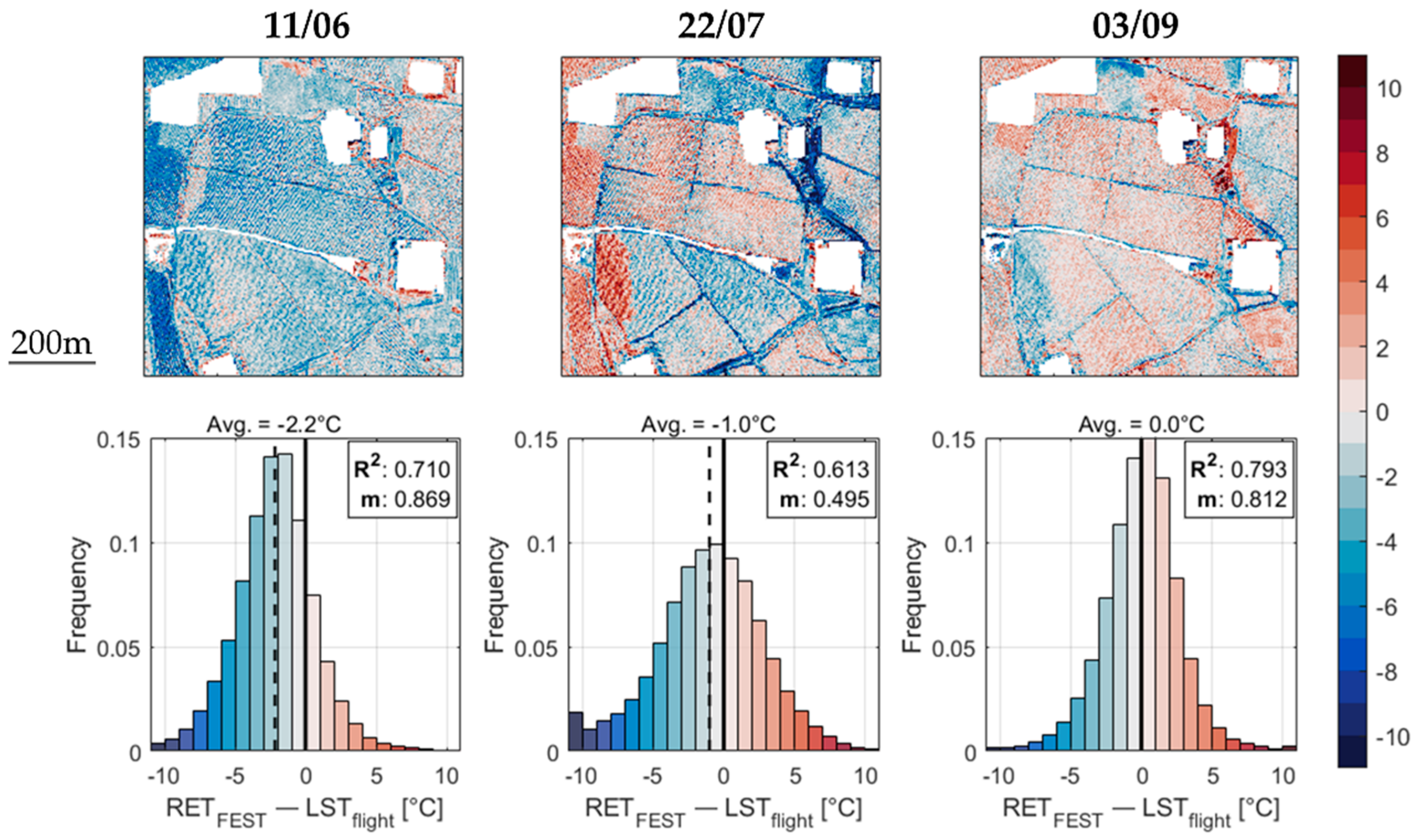
The calibration of the FEST-EWB distributed hydrological model has been performed by means of a pixel-by-pixel comparison between the modelled Representative Equilibrium Temperature (RET) and the remotely-sensed Land Surface Temperature (LST). The calibration process is regulated by the pixel-by-pixel minimization of the average model error, defined as the objective function O (Equation (2)).
O = def 1 n · i = 1 n ( R E T i L S T i ) ,
where n stands for the total number of calibration dates selected. The pixel-by-pixel approach of the calibration process allows to refine the spatial heterogeneity of the calibration parameters involved.
In previous applications of the model [48], four main parameters have been found to be critical for the calibration process: the Brooks–Corey (or pore-size distribution) index, the saturated hydraulic conductivity, the soil depth and the minimum stomatal resistance. Of these, the first three are mainly related to water geodynamics, while the latter is more closely connected to the ET process. As the daily simulations are performed in summer days with no precipitation or irrigation, offering a restricted time window, they are not enough to capture the water dynamics influenced by the former three parameters detailed above, thus decreasing their relative influence in the model performance for this particular application. Hence, it has been decided to calibrate the model working only on the minimum stomatal resistance, given its strong link to the energy partition mechanisms.
Furthermore, some preliminary analyses have shown that also the soil surface resistance (employed in the computation of the soil latent heat) needs to be considered in the calibration. This decision is motivated by the fact that highly heterogeneous canopy structures, like a vineyard’s, create complex air and heat patterns in the zone between the soil surface and canopy roof. These complexities are strongly influenced by the unvegetated areas between the vine rows, which are clearly visible to the model thanks to the high data resolution (1.70 m against the inter-row space of 2.40 m). Thus, the role of the non-vegetated areas among the vine rows needs to be properly addressed by its own soil resistance term in the energy balance equation.
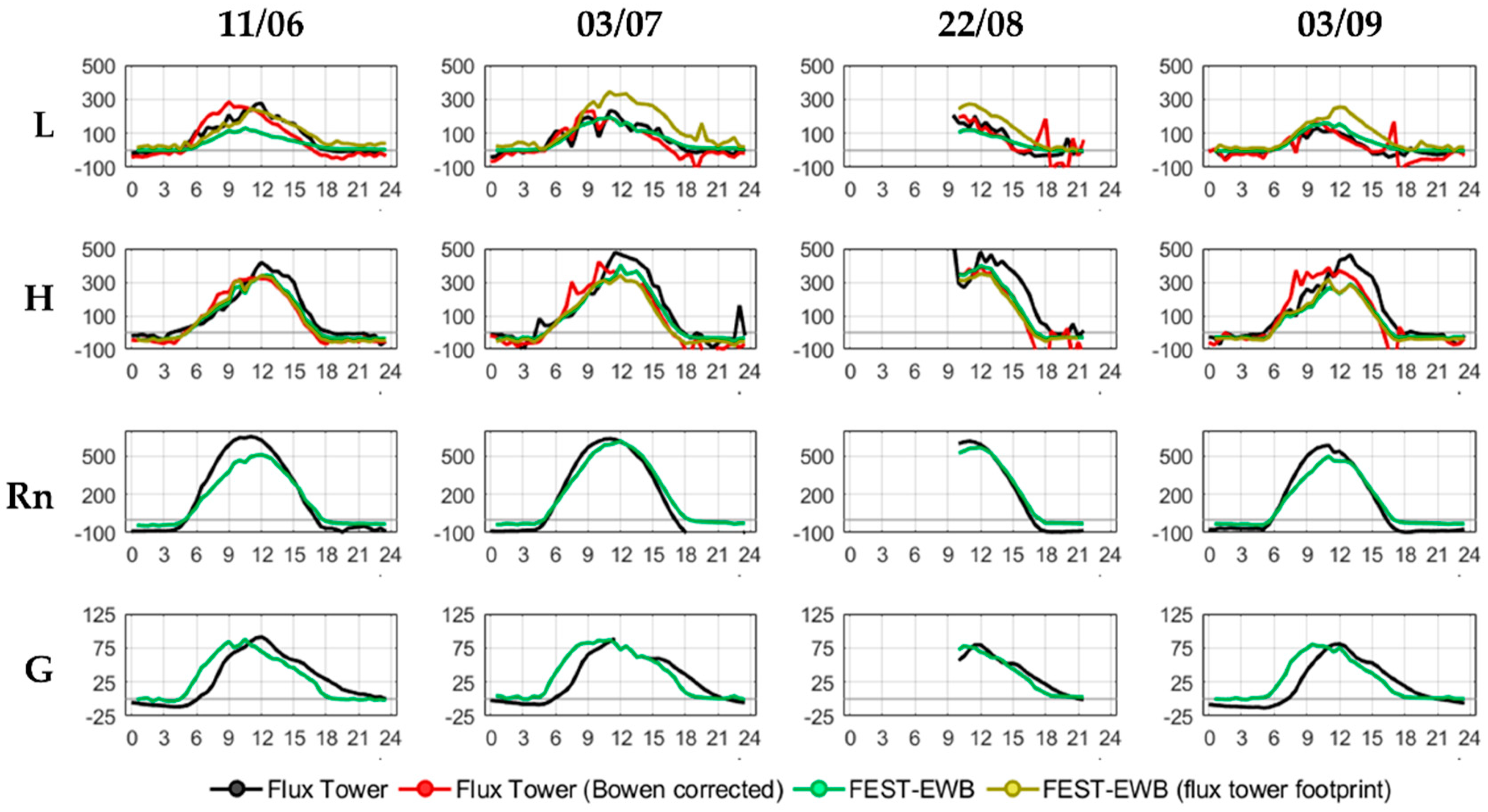
The possibility to calibrate the model using LST and validate it using energy fluxes obtained from an independent source allows a synchronous calibration/validation process. All energy fluxes are involved in the validation process: Net Radiation, Soil Thermal Flux, Sensible Heat and Latent Heat.
In the validation process are also included, as a reference, two widely-used and established energy models: SEBAL [23] and TSEB [10]. They belong to two distinct categories of energy balance models: single-source and two-source, respectively [50]. The former portrays each pixel as a homogeneous area, with a single energy balance equation (Equation (3a)) where the Latent Heat can be obtained residually after obtaining the Sensible Heat as a function of the radiometric/aerodynamic temperature TOH [K] and the aerodynamic resistance RAH [s m−1] (Equation (3b)).
L = R n G H ,
H = ρ C P T O H T A R A H
The two-source models, such as TSEB, partition the energy balance into two distinct equations, one referring to the non-vegetated (Equation (4a)) and the other to the vegetated fraction (Equation (5a)) of the given area. Sensible Heat exchanges are differentiated through a transition zone at air canopy temperature TAC [K], before being summed to gather the overall flux from the pixel. Latent Heat from the canopy (LC, W m−2) is obtained from potential-state formulations, such as Priestley-Taylor’s [51], while its bare-soil counterpart (LS, W m−2) is obtained residually.
L S = R n S G H S ,
H S = ρ C P T S T A C R S ,
L C + H C = R n C ,
H C = ρ C P T C T A C R X
Being the FEST-EWB structure somewhere in between these opposite approaches, these models have been considered in the analysis in order to provide a well-established reference for the FEST-EWB performance. The results used for the comparison are provided by [39], working on the same input data as those employed for the FEST-EWB runs.

2.2. Scale Analysis

The original data employed in this study are obtained by airplane flight and are characterized by a spatial resolution of 1.7 m, relatively high in the field of agricultural applications of remote sensing [
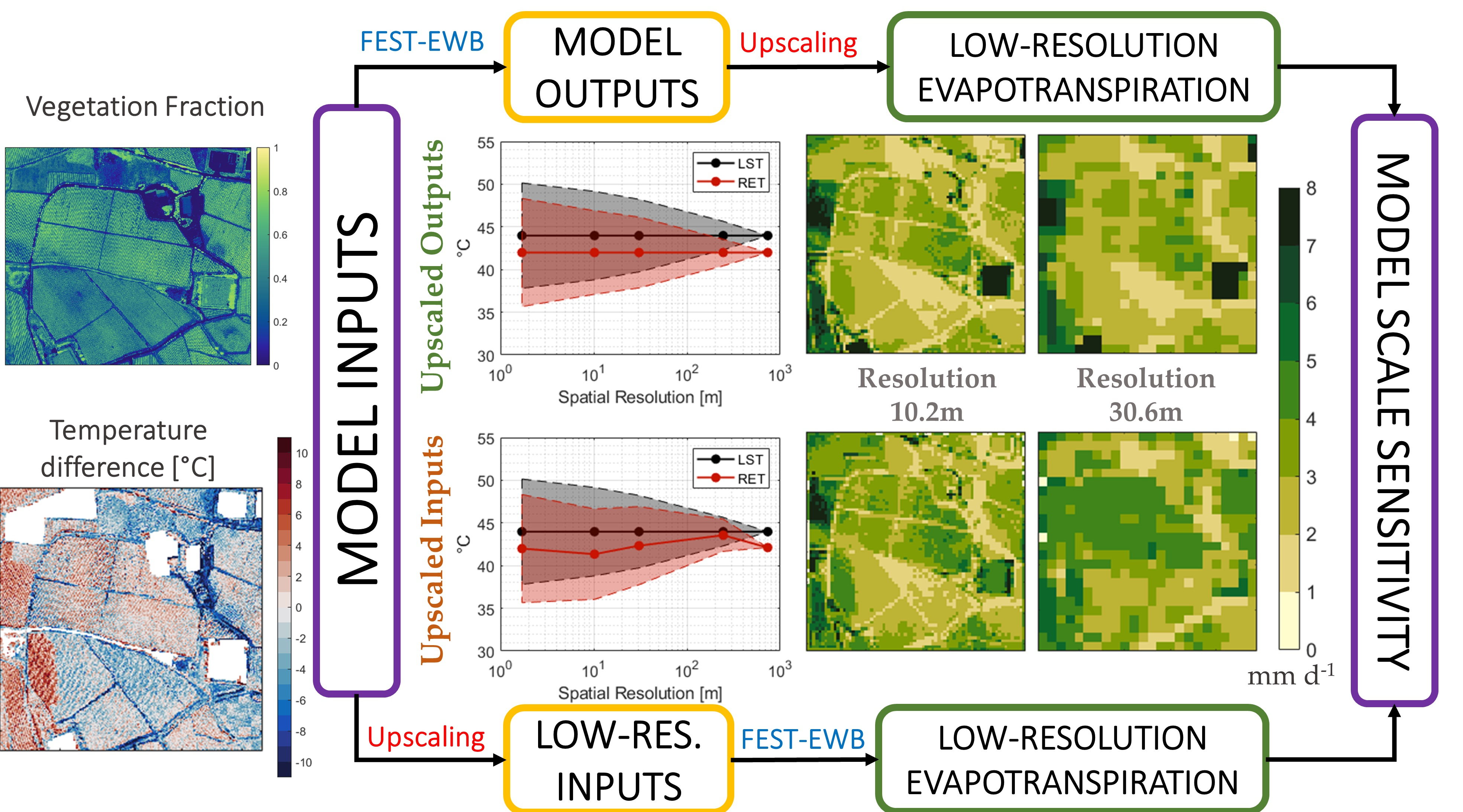
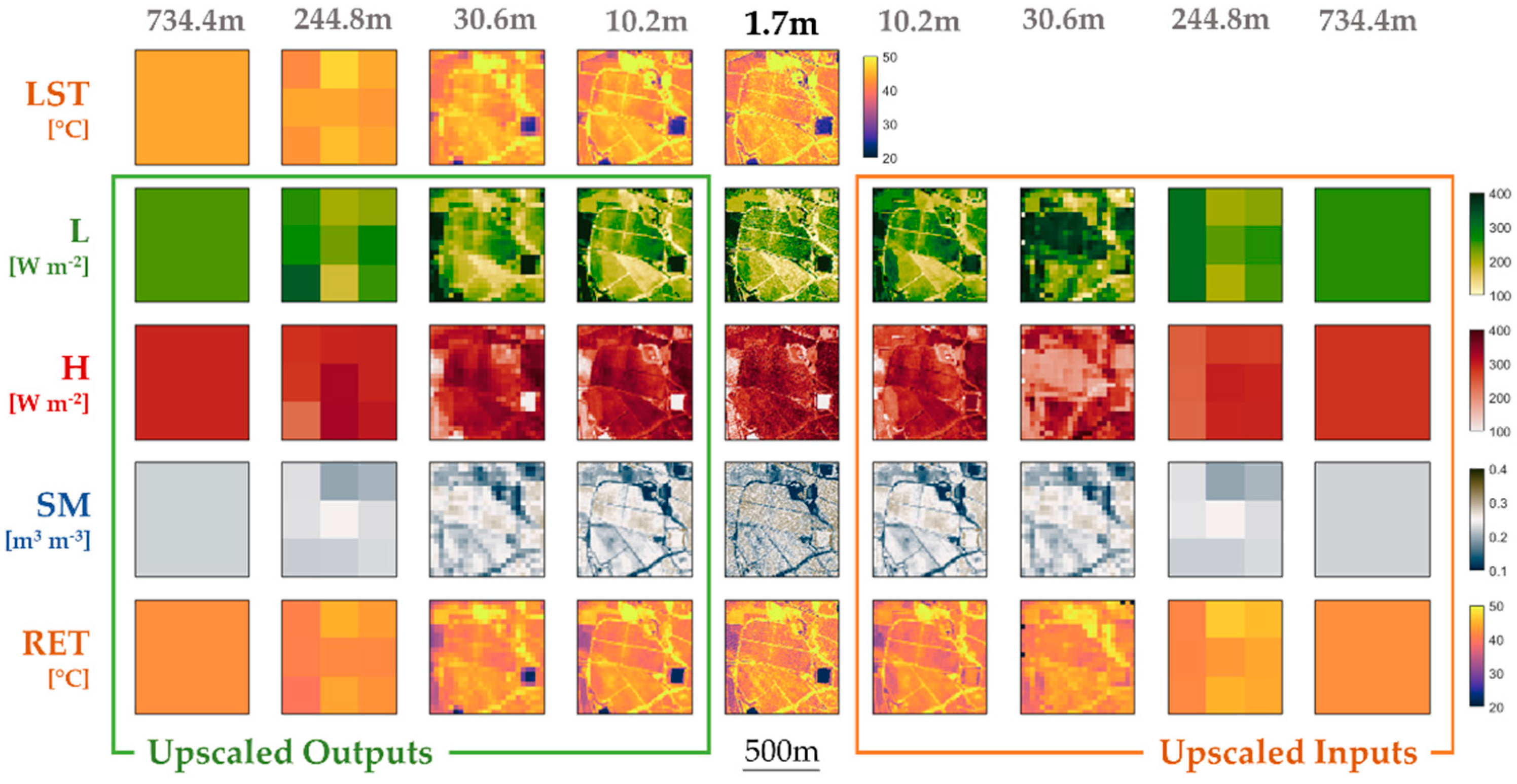
52]. The importance of spatial resolution has been tested on the FEST-EWB through scale analysis (Figure 1). Firstly, the model outputs (latent and sensible heats, soil moisture and representative equilibrium temperature) have been upscaled to some specific spatial resolutions (Section 3.2). Then, the input data have been aggregated to the same scales and fed to the model, which is calibrated anew for each spatial resolution employing the same calibration function of the highest-resolution calibration (Section 3.3). The model results, either originated from the upscaling of the native-resolution results or after the model calibration employing upscaled input data, have then been compared.
The scales chosen for the analysis have been selected by similarity with those of some common satellite products: 10 m for Sentinel-2; 30 m for Landsat multispectral; 250 m for MODIS Visible and 1000 m for MODIS Thermal. To avoid reprojections that could alter the original data, the target scales are picked among the multiples of the native scale (1.7 m): 10.2 m for similarity with Sentinel, 30.6 m with Landsat, 244.8 m for MODIS Visible and 734.4 m (the total extension of the area) for MODIS Thermal.
The upscaling has been performed through simple averaging of the original data to the target resolutions. The process is detailed in the following, as a nominative example, for the production of the 10.2 m upscaled product. The ratio (6:1) between the target (10.2 m) and native (1.7 m) spatial resolutions indicates that any target pixel covers 36 (6 × 6) native pixels. The value to assign to the target pixel is obtained as the average of the 36-pixel sample. For each sample, also the standard deviation is retained as an indirect measure of the pixel heterogeneity. Thus, for each final product, both an average and a standard-deviation map are stored. The process is repeated, always starting from the native 1.7 m spatial resolution, for all the scales involved in the analysis.

2.3. Case Study and Data Overview

The study area is the experimental vineyard field of the “Tenute Rapitalà” farm in the territory of Camporeale (Sicily, Italy). Data for this study have been collected during the June–September 2008 “Digitalizzazione della Filiera Agro-Alimentare” (DIFA) field campaign described in [39,40].
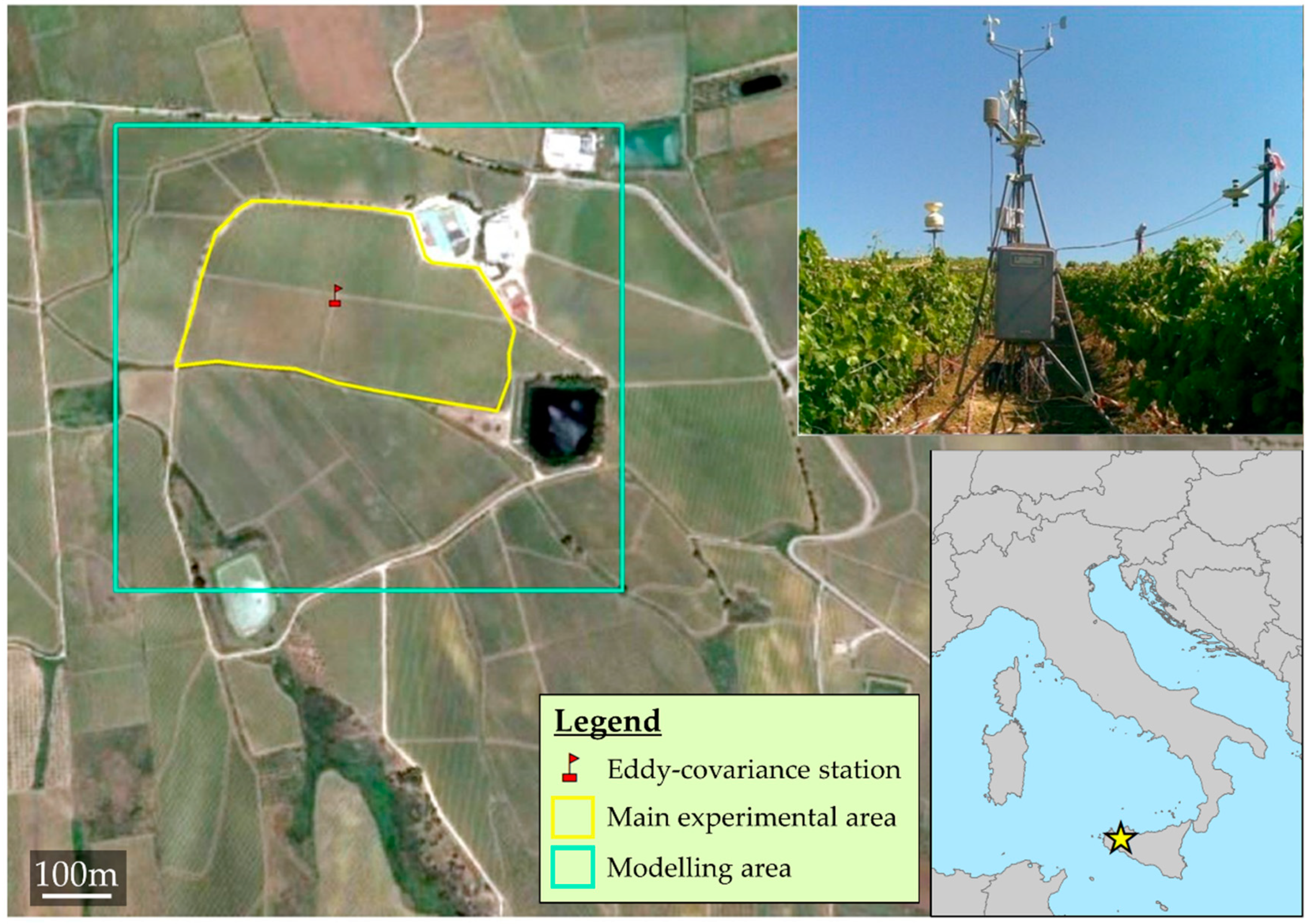
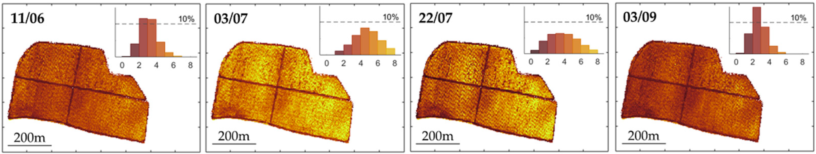
The case study is shown in Figure 2. The cyan square identifies the modelling area, while the central yellow-bordered area identifies the main experimental field, composed of four sectors separated by two cross-positioned paths. This main area hosts the eddy covariance station (photo provided in the upper-right corner) and is thus the main focus for the comparisons with its data. The vineyards are organized in rows 2.4 m apart; in each row, the single plants are positioned every 0.95 m, resulting in a global plant density of 4386 plants per hectare. The terrain shows a mild slope (<10%), oriented towards S-SW. The soil texture is classified as loam (20% clay, 29% silt and 51% sand), with 1.7% organic content. Residual Water Content (RWC) is estimated at 0.04 m3 m−3, whereas Saturation Water Content (SWC) is estimated at 0.45 m3 m−3 [53]. Drip irrigation is the main irrigation practice for the area.

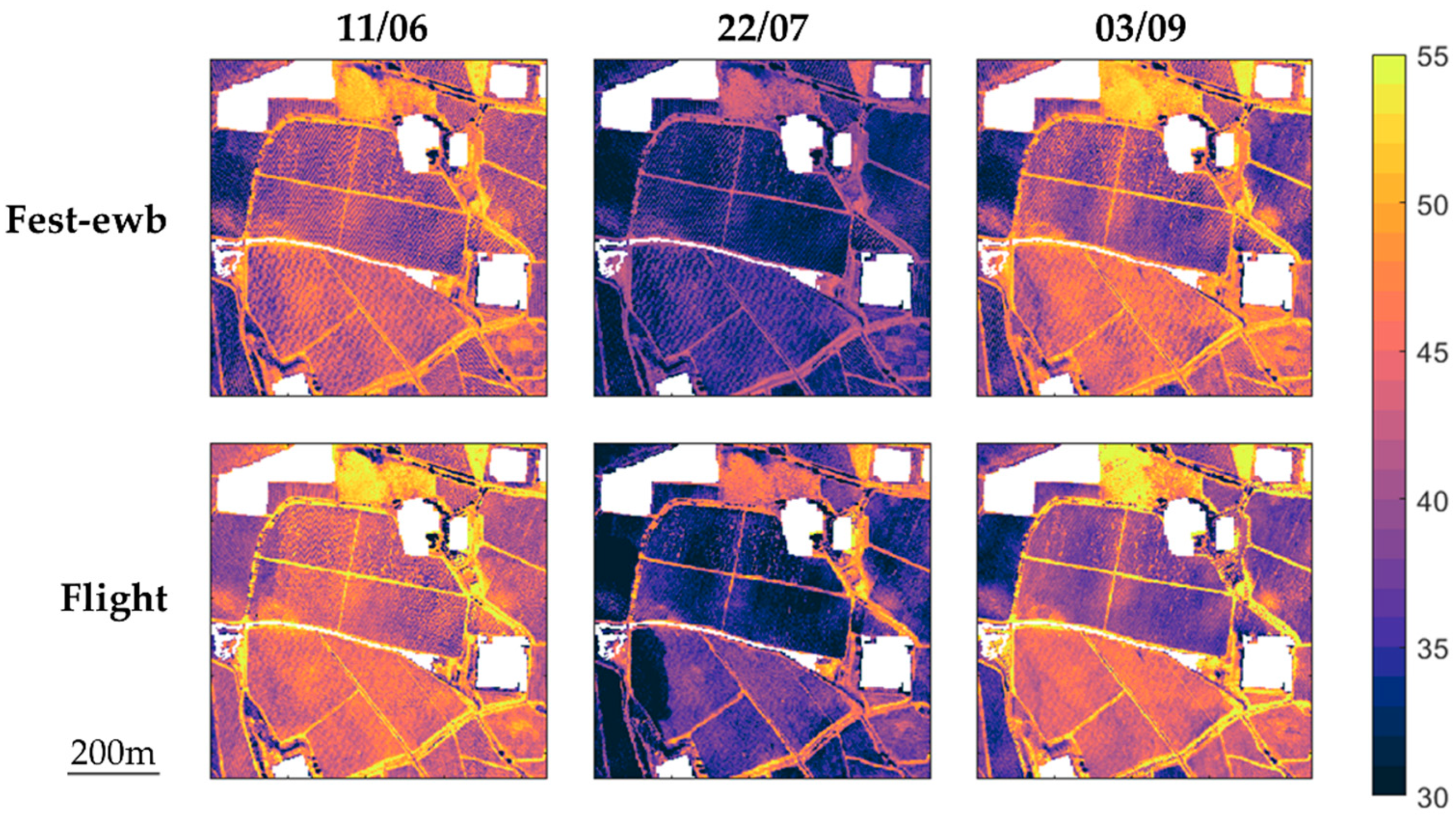
2.3.1. Airborne Proximal Sensing Data: Acquisition and Radiometric Calibration

Five remote sensing acquisitions have been carried out during the summer of 2008, using the airborne platform SKY ARROW 650 TC/TCNS with a sampling height around 1000 m above ground level. A multispectral Duncantech MS4100 camera operating in the 767–832, 650–690 and 530–570 nm bands has been used to retrieve the visible (VIS) and near-infrared (NIR) images; a Flir SC500/A40M camera, working in the 7500–13,000 nm band, provided the thermal infrared (TIR) images. This distinction resulted in a different nominal pixel resolution for the VIS/NIR data (0.7 m) and the TIR data (1.7 m). The original data have been aggregated at 1.7 m using a pixel aggregate method. Thus, the 1.7 m spatial resolution is assumed as reference resolution for scale effects analyses.
The flights were been carried over in 5 days in 2008: 11th June (DOY 163), 3rd (185) and 22nd (204) July, 22nd August (235) and 3rd September (247). These days were all characterized by optimal meteorological conditions to improve the quality of the data collection process.
Further details on the thermal image pre-processing are discussed in Appendix A.
Leaf Area Index (LAI) and vegetation fraction (fV) data have been gathered employing LAI-2000 Plant Canopy analyzer, an optoelectronics instrument. Plant height information has been obtained from NDVI data by means of an empirical relation calibrated in situ.

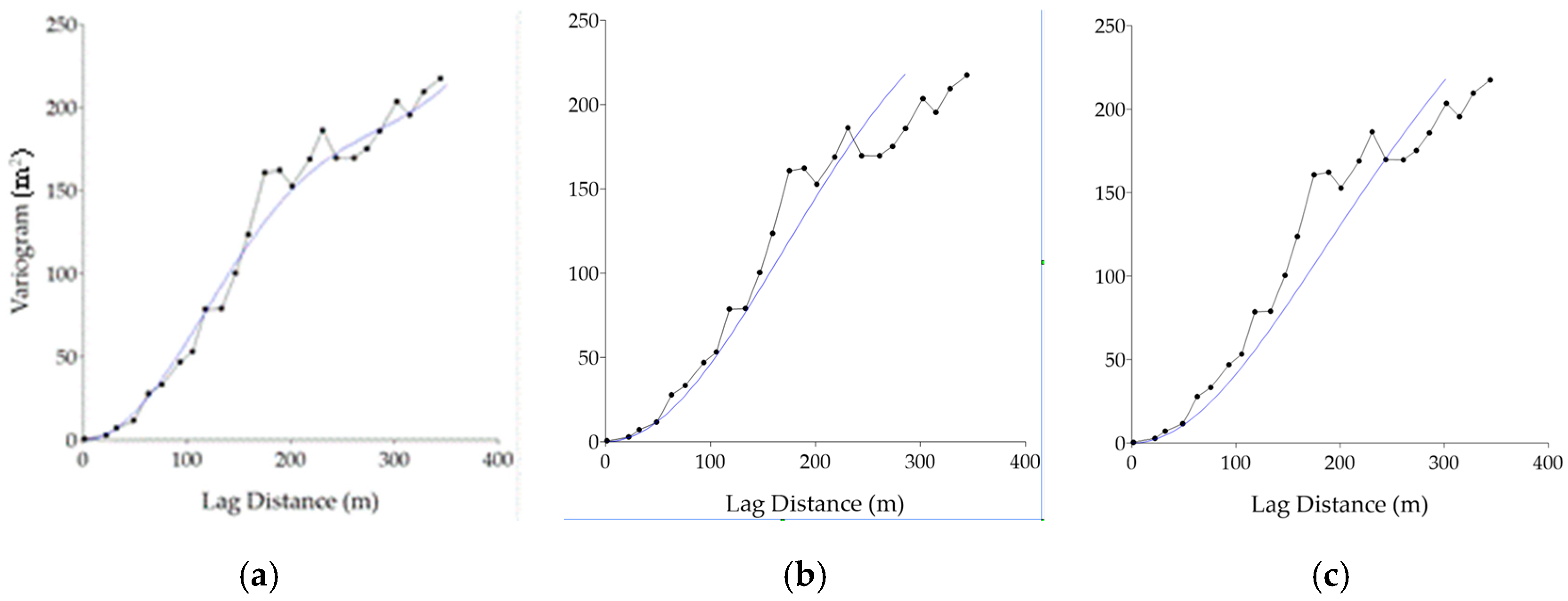
2.3.2. Digital Elevation Model: GNSS Acquisitions and Geostatistical Analysis

The digital elevation model (DEM) was obtained by interpolating orthometric altitudes measured via GNSS (Global Navigation Satellite System). A GNSS receiver, namely a Topcon GMS-2, was mounted on a tractor allowing characterizing the study area altitude by running up and down along the middle of all the vineyard lanes.
A simple Differential GPS (DGPS) provided position solutions with accuracies comparable to the spatial resolution of the images (≈2 m).
Data were acquired on the 17th June (DOY 169) between 7:45 and 12:45 UTC at 5 s time steps, for a total amount of ≈3037 positions. Of these, 136 positions were removed to missing differential correction.
Further information on this pre-processing step is provided in Appendix B.

2.3.3. Eddy Covariance Data

A flux tower was located at the center of the experimental field for the entire duration of the monitoring period. The station is equipped to measure also air temperature and humidity by a sensor placed at 2.75 m above ground and a pluviometer, with 0.2 mm accuracy, installed at 2 m above ground. The eddy covariance setup included a CSAT3 sonic anemometer and an open-path LICOR-7500 IR Gas analyzer operating at 3.40 m above ground and with 20 Hz measurement frequency, although the final data are provided with the 30 min time step common for these kinds of set-ups. The turbulent fluxes exchanges have then been estimated from the vertical wind covariance with several parameters: the air temperature (to determine the sensible heat), the water vapor density (for the latent heat) and the CO2 density (for the carbon dioxide flux). A detailed description of eddy covariance data analysis is provided in [40].
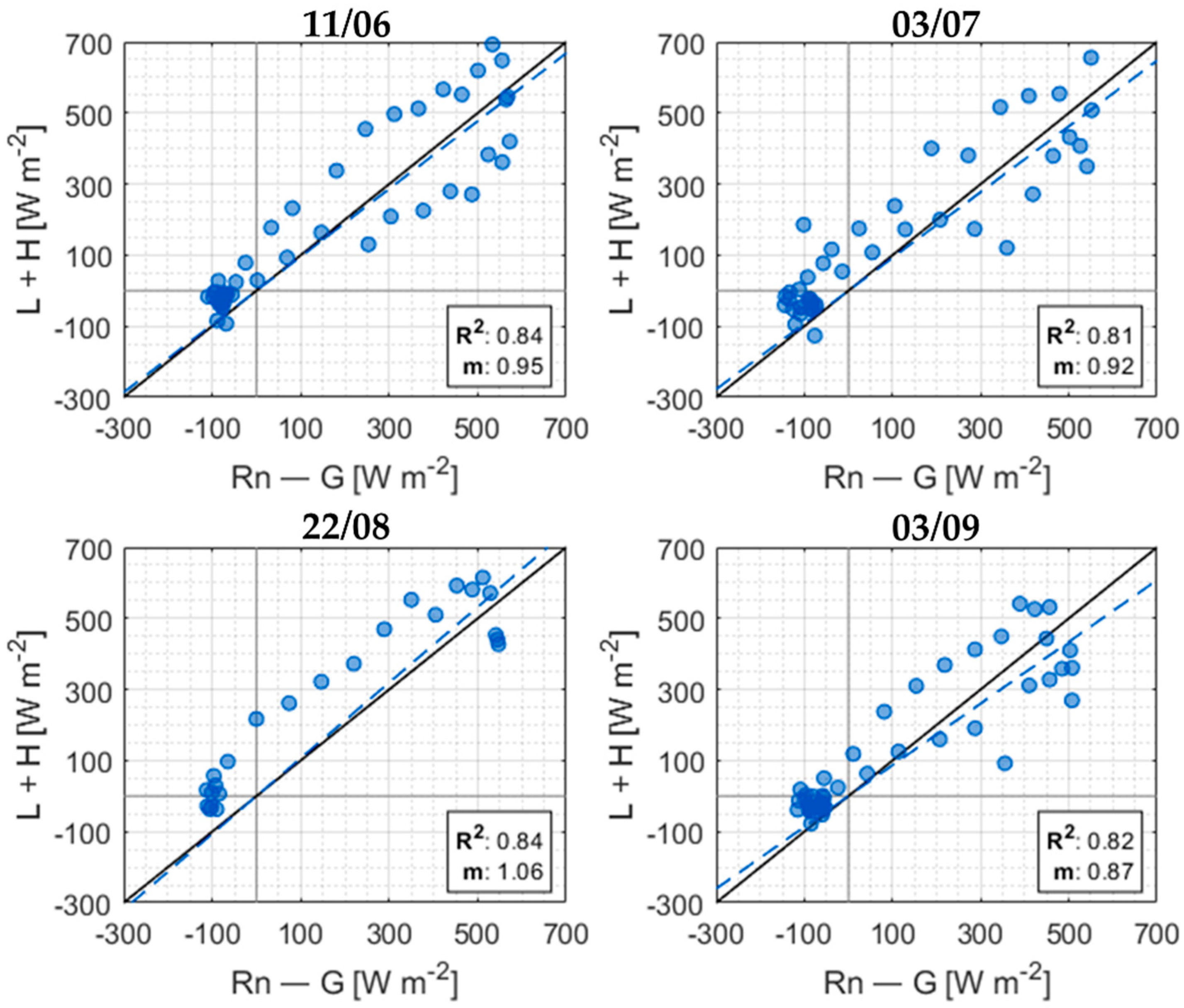
At each time step, the four components of the energy balance are then available: Net Radiation (Rn), Soil Thermal Flux (G), Latent Heat (L) and Sensible Heat (H). The closing of the energy balance is summed up in the average angular coefficient of the energy-balance interpolators, estimated at 0.95, together with the data dispersion value, averaging 0.83. This is consistent with the fact that, when measured with eddy covariance stations, the energy balance is not closed by definition, as the available energy is always higher than the turbulent fluxes (as well known in literature: [54,55]). More insight into the energy closure plots for each measurement day is provided in Appendix C. Due to the nature of surface energy balance models, which are based on the closure of the energy budget, the eddy data must be corrected by distributing the error among the turbulent fluxes according to the Bowen ratio to force the closure of the energy balance [56]. However, because of some low-quality long-wave radiation data, the corrected Latent and Sensible Heats may become out of phase with respect to their “expected” peak time. This issue will be explored more in depth in Section 3.1.2.
Data measured from eddy covariance stations generally do not refer to the single point in space in which the instrument is placed, but are influenced by the aerodynamic conditions of the atmosphere bottom layer in which it is located. An approximate analytical model has been developed [57], to simulate the measurement distance of an instrument for given atmospheric conditions. This model has then been expanded in a bidimensional formulation to compute the areal footprint of the eddy covariance measurement [58].
Local micro-meteorological conditions determine how wide the area that contributes to the actual measure is. For our case study, average day-time conditions determine that 90% of the eddy footprint area covers 10 ha. According to the data spatial resolution, these numbers can mean that a footprint computation is required to aptly simulate the measurement performed by the instrument. Lower resolutions cover most of the footprint with only one pixel, meaning that the simple pixel value is enough for the comparison with the eddy station measurements.

2.3.4. Global Data Overview

The information about the employed data is summed up in Table 1.
Energy fluxes information was unavailable for 22nd July, disqualifying it as a feasible date for the validation step. Meteorological and energy fluxes data for 22nd August were available only for the 10:00–21:30 time range, implying that the conditions at the time of the flight overpass (09:15) could not be simulated using FEST-EWB. This means that this date could not be included in the calibration. Finally, data from 3rd July have been excluded from the calibration step because of incongruencies in the reported flight time with usual registered LSTs. Turbulent flux data, on the other hand, are employed in the validation process. As already stated in Section 2.1, data are available only on single flight dates. Because of this restriction, no continuous model run could be performed. Instead, single daily simulations were executed.

3. Results

3.1. FEST-EWB Calibration/Validation

3.1.1. Calibration

As stated in Section 2.1, the short daily simulations without any precipitation nor irrigation do not allow the possibility for the model to capture the water dynamics influenced by the soil calibration parameters. Hence, the calibration has been restricted to two parameters linked to the evapotranspiration process: the minimum stomatal resistance (rS,min) and the soil surface resistance (rS). These parameters have been corrected across numerous simulations with the aim of minimizing the temperature error, as detailed in the “Calibration and Validation procedure” section. The results of this calibration are detailed in Table 2. Originally, soil surface resistance was set to 500 s/m for all the pixels; minimum stomatal resistance, on the other hand, was set to 200 s/m for highly vegetated pixels and to 50 s/m for the remaining pixels, based on the well-established literature values for vineyards and grass patches, respectively.
The comparison between modelled RET and estimated LST is shown in Figure 3 for the three calibration dates. The results show a good correspondence, especially in the distinction between warmer bare-soil areas and cooler vegetated patches. Some areas have been blanked out, as they are not pertinent to the analysis (artificial basins, tarmac, and buildings).
Model biases (difference between modelled RET and estimated LST) are plotted in detail in Figure 4, both in map and histogram formats. Model errors seem to be normally distributed around their average value, with most of the pixels (61%, 59% and 78% for each date, respectively) displaying an error within ±3°C of the target LST. For what concerns the spatial distribution of the error, different trends are visible for each date. While 11th June seems to have a uniform error distribution, 22nd July shows important underestimation-errors in the non-vegetated areas, and 3rd September displays a diffused overestimation in the vegetated part. In all three dates, however, some “spot”-like errors are present, mostly found in the western part of the image. For these “spot”-like areas, the model error seems to be distinguished from that of the nearby area: on 11th June, the model is much cooler than the LST in that area with respect to the central part of the test site, and on 22nd July, a sudden change in the model trend (from a sharp overestimation to a mild underestimation) is clearly visible. These problems may be due to the nature of the LST images employed, which are the result of a composition of different passages of the same airborne instrument over the area. Thus, some areas, although geographically close, can be sensed by the instrument in similar, but different, time intervals; a cloud temporarily obscuring the sun can then be enough to produce a sharp temperature difference between relatively close areas. The extent of these areas can be assessed in the original LST images from Figure 3. On the other hand, some discontinuities in the RET distribution can also be detected for 11th Jun and 3rd Sep. These may be linked to similar image composition problems in the input vegetation data.
The adaptation statistics for the calibration process are detailed in Table 3. On the left-hand side of the table, classic adaptation statistics are displayed: model-to-data bias (B), slope of the linear regression (m) and determination coefficient (R2). On the right-hand side, the surface temperature error (expressed in terms of Root Mean Square Error, RMSE) is sorted by vegetation degree (in terms of Leaf Area Index, LAI) of the relative pixel. Generally, lower errors are found for medium-to-high vegetation levels, although the 11th June test date shows a less definite trend.

3.1.2. Validation Results

Among the FEST-EWB results, components of the energy balance for each pixel are available. These outputs can be compared with the quantities measured by the eddy covariance instruments, as detailed in Figure 5. For the modelled turbulent fluxes (L and H), both information extracted for the eddy footprint area and data from the station pixel itself are provided. For the purpose of validation, both original (black line) and Bowen-corrected (red line) eddy covariance data are shown for both Latent and Sensible Heat. The corrected ones appear out-of-phase with the others, as a result of some problems with the longwave radiation data. These have been employed for the validation statistics detailed below, but original data have been preserved in Figure 5.
In the lower panels, Net Radiation (Rn) and Soil Heat Flux (G) are compared, with positive results, although a slight out-of-phase relation between modelled and measured fluxes is noticeable, in particular for the Soil Heat Flux. This, however, is consistent with the slight shift observed in the eddy station data, as mentioned earlier in Section 2.3.3, and can be blamed on some reference data inconsistencies. In the upper panels, Latent and Sensible Heats are displayed. The green line details the flux modelled in the station pixel; the yellow line depicts the average flux in the station footprint area. As detailed in Section 2.3.3, the physics of the turbulent flux measurement require knowledge of a certain footprint area, highly dependent on the meteorological conditions, such as wind intensity and direction and atmospheric temperature. The presence of a consistent bare-soil area around the station is evident in the higher values of the Sensible Heat as opposed to the Latent Heat registered by the station. These dynamics are all well-captured by the model interpretation.
The visual adaptation shown in Figure 5 is detailed in Table 4 with some common statistics. Linear interpolation slope (m), determination coefficient (R2) and Nash–Sutcliffe Efficiency (NSE) are provided for all the curves displayed in Figure 5. A comprehensive average column has been added to the right of the table. The turbulent fluxes are overall well-interpreted by the model (NSE > 0.5) when referred to the station pixel. As footprint filtration is introduced, model performances generally decrease (only the Latent Heat for 11th June presents a performance increase when employing the footprint). This may be attributed to the extremely heterogeneous conditions of the vineyard crop structure which constrains the flux tower measurements to its immediate vicinity by hindering water vapor (for latent heat) and heat (sensible heat) horizontal motion across the field.

3.1.3. Evapotranspiration Output

Modelled evapotranspiration for the main experimental vineyard area is also evaluated. The modelled ET is presented for the main experimental area, in form of histograms and spatial distributions, in Figure 6. Bare-soil paths are clearly visible in every date, together with an alternance between high- and low-ET pixels in the vine rows area.
The averaged values have been compared with others, as reported in Figure 7. First, the Flux Tower estimated ET, which is relative only to the flux footprint area. Then, the global area ET (as shown in Figure 6) is estimated by two energy-balance models already employed in the comparison in [39]: the single-source SEBAL and the two-source TSEB. The modelled results seem quite in line with those of the other energy-balance models. This may be explained by the presence of vegetation (low grass) in the vines interrow, which participates in the overall evapotranspiration. The overall area, although not homogeneous, is less heterogeneous and can thus be portrayed with comparable accuracy by models with approaches both “extreme” to one another (SEBAL and TSEB) and “hybrid” between the two (FEST-EWB). Flux Tower results are quite low, with respect to the modelled ones, for the 3rd Jul and 3rd Sep dates. This can be explained by the fact that, in those days, the dominant wind direction is WNW, which is partially aligned with the main bare path, reducing the overall measured daily ET. By also displaying the eddy-pixel modelled data, without accounting for the station footprint, results similar to those measured by the eddy can be detected for the dates of 3rd July and 3rd September, while an underestimation is observed for 11th June. This could be explained by particularly turbulent conditions in the proximity of the station, which caused the station to measure quantities much more in its immediate vicinities. Thus, its measured value results are much closer to that of the station pixel than that suggested by the eddy station footprint theory. These results reflect the time series displayed in Figure 5, and the performance statistics detailed in Table 4, with low NSE values for the footprint-corrected data in the July and September dates (negative values) and higher values for the uncorrected modelled values (bigger than 0.5).

3.2. Upscaled Outputs (UO)

The aggregated maps employed in the scale analysis are shown in Figure 8. In the example 11th June date (11:00 local time): airborne-sensed Land Surface Temperature (LST), Latent Heat (L), Sensible Heat (H), Soil Moisture (SM) and Representative Equilibrium Temperature (RET) are shown. The results of the Upscaled Outputs approach are displayed on the left-hand side of the image. It appears that some surface heterogeneity features (e.g., bare-soil paths) are clearly preserved in the first step (10.2 m) and still distinguishable in the second (30.6 m), where the scale ratio is 18:1. From the third step (244.8 m) all heterogeneity is lost. The information degradation process that follows the aggregation is also visible when comparing the LST and RET evolution. Although the colors suggest slightly different values, the obliteration of the field-characterizing features is definitely similar.

Data Variance across Scales

In Figure 9, the evolution of the frequency distribution for the same data displayed in Figure 8 for 11th June (11:00) across the different scales is detailed. The first row displays the Upscaled Outputs results. FEST-EWB RET and flight-gathered LST (Figure 9a), modelled Latent and Sensible Heats (Figure 9b) and modelled soil moisture (Figure 9c) are shown. For each plot, the darkened area identifies the one-standard-deviation-range (±σ) around the average value. As scales progress, the overall data average is unaffected, whereas fewer pixels covering the same area determine a decreasing heterogeneity of the data. As the 734.4 m step is made up of just one pixel, all standard deviations are null at that stage.
In Figure 9a, the positive model interpretation of the LST transpires from the similar shape of the two plots. The bias that separates them at the native resolution, detailed in Table 5, is preserved along the aggregation process. In Figure 9b, it can be observed how Latent Heat tends to be more widely distributed than Sensible Heat. This distinction holds until the 30.6 m threshold, with the two fluxes gaining similar heterogeneity by the 244.8 m step. This is consistent with the observations in Figure 8, where the heterogeneity features are shown to hold until the 30.6 m upscaling step. The entity of these heterogeneity shifts is detailed in Table 5. For each product and each scale, the variation coefficient (standard deviation normalized with the average value) is shown, progressively decreasing with the increase of the spatial resolution.

3.3. Upscaled Inputs (UI)

In the second part of the scale analysis, data inputs have been upscaled to the different target scales before being employed in the model. Thus, after calibration, the model results are produced directly at the target scale, simulating the functioning of the model at coarser resolutions for the same data set. In order to identify the heterogeneity loss with spatial resolution of the model inputs, some of them are described in Table 6. Heterogeneity information is presented in terms of Variation Coefficient for all scales except the coarser (744.8 m), for which only one pixel is available. Since the aggregation is performed with the simple averaging approach, the average value of each parameter is preserved, just like the UO results. Variation coefficients decrease to about one fourth of their highest-resolution value by the last scale step, indicating a quite uniform data levelling for the model input.
A similar effect is visible on the calibration parameters, and is detailed in Table 7 for all the calibration steps. The Variation Coefficient stays high (above 50%) until the 30.6 m step, before plummeting to the 25% value of the 244.8 m scale. The calibration functions employed for the two parameters are practically the same, except for overestimated values. This distinction brings about different calibrated datasets until the 10.2 m step. By the 30.6 scale, the most extreme overestimations have been smoothed out, and the two parameters converge to similar distributions.
The scale evolutions for LST, RET, Latent Heat, Sensible Heat and Soil Moisture are portrayed in Figure 9 (lower row) for 11th June, 11:00 local time, with the relative variation coefficients detailed in Table 5. Turbulent fluxes (Figure 9e) show similar behaviors to those of the upscaled outputs (Figure 9b), with smaller variation coefficients, in particular in the Latent Heat and the higher-resolution steps. This may be attributed to the loss in spatial heterogeneity caused by the upscaling process: working on less heterogeneous input data, the model provides less heterogeneous outputs. Analyzing the values in Table 6 and those in Table 5, it can be observed that, for the 10.2 m and 30.6 m scales, UI Latent Heat presents six-tenths of the diversity shown by its UO counterpart. However, the former is originated from the input data with six- to seven-tenths of the heterogeneity of the UO one.
These concepts are less visible for the Soil Moisture, as evident by the similarity between Figure 9c and Figure 9f. The difference is minimal, being slightly perceptible only in the numbers in Table 6, because of the reduced soil moisture dynamics due to the brevity of the simulated period. Most pixels retain values very close to those of the starting condition, which is obviously uninfluenced by the upscaling approach.

3.4. Approaches Comparison

3.4.1. Temperature Biases

Figure 10 displays the summed-up surface temperature results for the two upscaling approaches. Green dots identify the average temperature biases (model RET against flight LST) obtained by upscaling the model outputs. The green area highlights the one-standard-deviation-range around the mean value (±σ). As already discussed, the averaging process preserves the global mean. On the other hand, the orange dots provide the average temperature biases for the upscaled-input model results, with the orange areas identifying the standard deviation range as above. The independent calibrations that produce the upscaled-input results, although completely unrelated to the upscaled-output data, provide quite similar temperature biases. For high resolutions (10.2 m and 30.6 m), the average biases are particularly similar to the upscaled-output results. Coarser resolutions lose some of that similarity (in particular on 3rd September), but the overall comparison of the two datasets remains remarkable. Generally, low (absolute) biases can be attained with either of the upscaling approaches, as in both, the error-minimization calibration rationale is employed.

3.4.2. Global Evapotranspiration

The comparison between the two approaches is investigated also in terms of daily evapotranspiration, focusing on the main vineyard area. Figure 11 provides the absolute-value results of this comparison in the left-hand column. The golden bar identifies the calibrated-model ET result for the native resolution; the green bar identifies the upscaled-outputs approach result, whereas the orange one is the upscaled-inputs result. The UO and UI results are never equal, but they are fundamentally never far from each other. Varying on the days, the differences can be more or less marked, but the overall value is similar, with no clear over-estimation of one over the other. Furthermore, both values are generally in the vicinity of the daily ET computed at the highest resolution (the golden bar). This aspect is further investigated in the right-hand column of Figure 11, which displays the Relative Error (RE), for both approaches, between the ET valued at the coarser scale and the highest-resolution ET assumed to be the most accurate. The green line identifies the UO approach again, and shows an error increasing monotonously and coherently with the simple averaging method at its origin. The line for the 3rd July, although seemingly constant at the null value, presents non-null errors, poorly distinguishable as always below 1%. The orange line represents the UI results, with a more erratic scale evolution, as already seen in Figure 10 for the independent calibrations. The RE data are useful because of the limited variability of the ET values, which hinders a clear understanding of the possible error. The results shown confirm this assumption, as non-negligible errors as high as ±30% can be detected. Generally, UI errors are higher than those of UO, but, being subject to calibration, can be even lower (as is the case for the 734.4 m scale in the 11th Jun and 3rd Sep dates). While UO, by construction of the simple averaging methods, is monotonically increasing, UI has no pre-defined behavior.
Given the nature of the scale analysis, further insight into the effects of spatial resolution over model application can be obtained by analyzing the spatial distribution, instead of the average value, of ET. Figure 12 shows the different ET spatial distributions across the four scales of our analysis, for the example date of 11th June and comparing both scaling approaches. For the 10.2 m scale step, little differences can be detected, in line with the average value featured in Figure 11. The pattern of slightly higher ET in the eastern half of the vineyard is visible in both approaches, while the western half shows some discrepancies between the two. In the shift towards the 30.6 m step, the different calibration of the UI approach is quite evident (as foretold by the higher average value in Figure 11), although spatial patterns start to fade out. The low-ET roads surrounding the vineyard are clearly distinguishable in both approaches, as the empty fields are directly north and south of the main vineyard area. Finally, in the 244.8 m step, both approaches seem to converge to similar values for the pixels involving the main vineyard area, as the lumped nature of pixels at this coarse spatial resolution flattens out most singularities in the target area.

4. Discussion

Numerous doubts regarding the scale issues with energy fluxes involve the common assumption of pixel homogeneity in most surface energy balance models [31]. These concerns revolve around the modelling of non-linearities, which do not cope well with the (often) linear aggregation processes. Non-linearities are all the more evident for heterogeneous pixels. Again, Ref. [31] focused on the dependency of modelling roughness lengths (used to compute aerodynamic resistances) on spatial resolution, postulating that all models following the Monin–Obukhov Similarity Theory (MOST) face this challenge.
The scale analysis shown in this study aims at testing the FEST-EWB sensitivity to modelling non-linearities across common spatial resolutions for a remote sensing product. Two approaches are contrasted: aggregating model results obtained at high resolution (Upscaled Outputs approach, or “UO”); aggregating model inputs before calibrating the model anew (Upscaled Inputs approach, or “UI”). Faced with this double approach, the FEST-EWB model has shown consistent results.
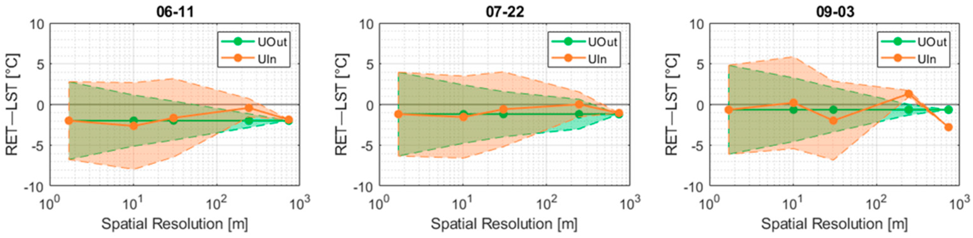
In the calibration phase (Figure 10), the temperatures are comparable between the two approaches. The calibration process, employing the same calibration functions for both approaches, was demonstrated to be only slightly hampered by the spatial resolution. This is all the more impressive provided the loss in spatial information brought on by the upscaling process, both in the actual results for UO and in the input data for UI, as testified by Table 6. Although data inputs become up to three-fourths less diverse, the model still manages, with the appropriate calibration, to provide low temperature biases. The aggregated fluxes (Figure 9) reflect this decreased data diversity with less heterogeneous UI latent and sensible heats with respect to their UO counterparts.
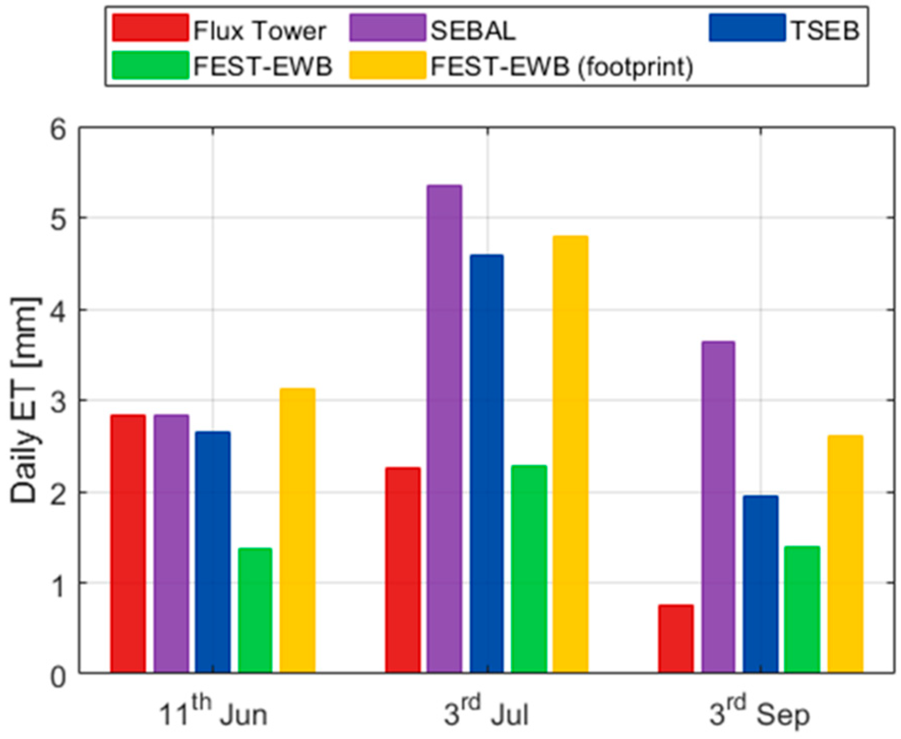
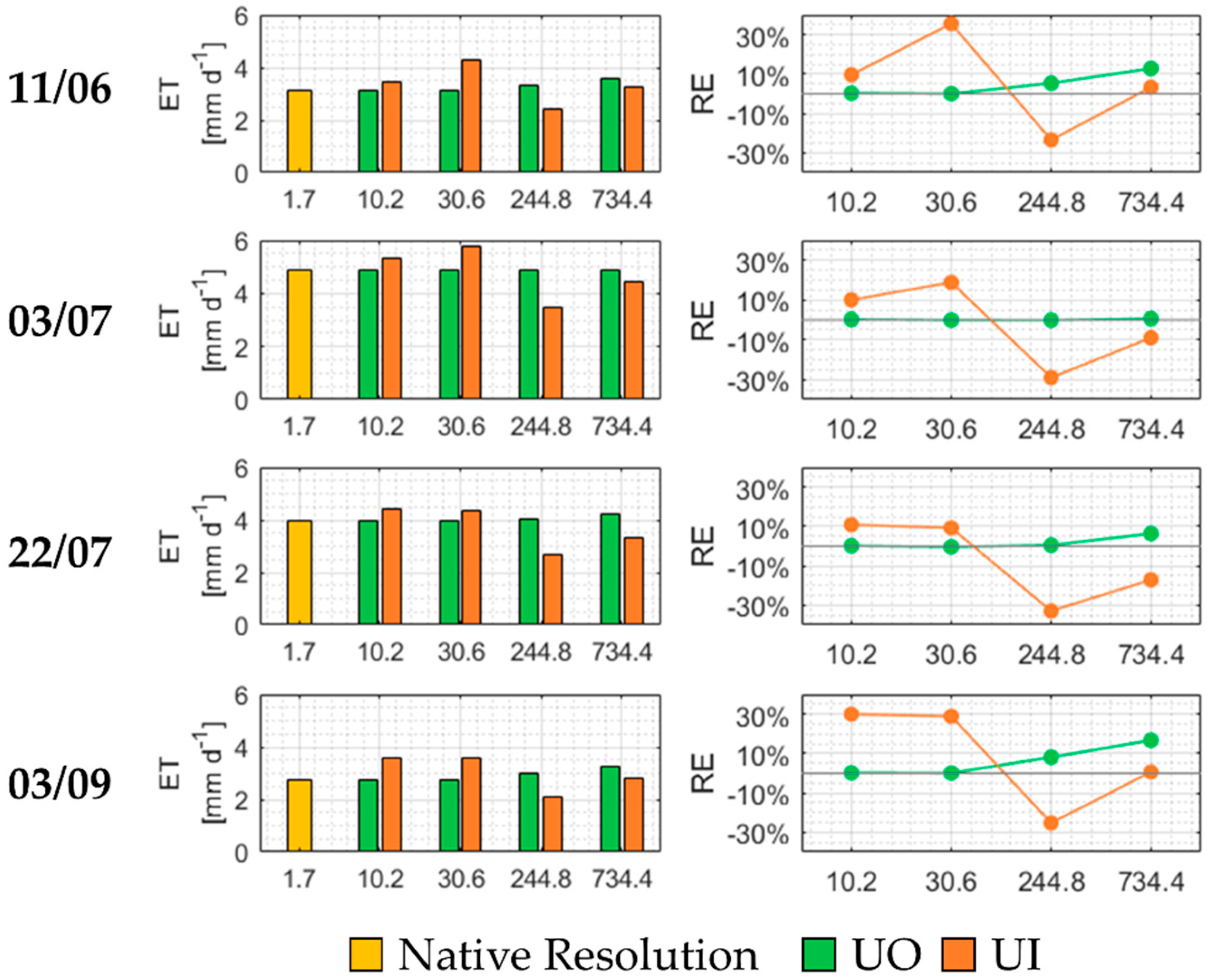
To provide an operative estimate for the model performance in coarser-resolution scenarios, ET global estimates for the vineyard area are computed with both approaches and compared to their high-resolution counterparts. This adaptation is detailed in Figure 11, with the two different scale evolutions for the UO and UI results. While the simple averaging approach provides a monotonous relative error increase in the UO scenario, the independent calibrations set a more erratic error distribution for the UI approach. Clearly, the UI errors appear overall higher than the UO ones, in agreement with [37]. They found that ET was better preserved with output upscaling than with input upscaling, as in the former case the coarser-scale ET relative error reached, at most, 28%, whereas in the latter it stretched just above 40%. The results of input upscaling for their work was obtained for a model (SEBS) which did not require calibration; probably for this reason, the upscaled-input ET showed a monotonously increasing error which is not the case for this study, as shown in Figure 11. The overall error values are, however, in tune with what was found in this study.
Some further considerations are due for the UI results shown in Figure 11. As the model is subject to a new calibration for each scale, low errors are theoretically possible even for coarse resolution, which is not the case for the UO results. However, as scales progress, fewer and fewer pixels cover the same area; in this case, only 1 pixel for the 734.4 m scale and 9 for the 244.8 m one. Fewer available pixels dramatically hinder the perks of employing a distributed hydrological model, as less parameter values can be tuned during the calibration process. Thus, while low relative errors are theoretically possible for coarse scales in the UI approach—as for the 11th Jun and 3rd Sep dates in this case, for the 734.4 m scale—the calibration process can provide worse results, as is the case for the 244.8 m scale.
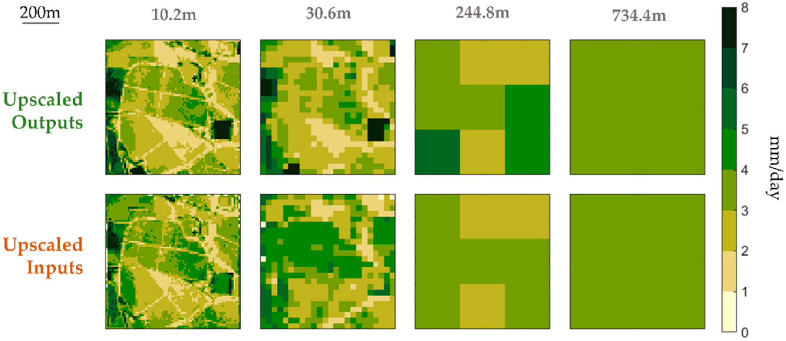
Finally, some positive insights of high resolution data can be gathered by the ET spatial patterns shown in Figure 12. The differences between the two scaling approaches seem quite in line with those of the averaged values discussed above. This is particularly true for the highest resolution of the scale analysis (10.2 m), the closest to the native resolution. As scales progress, some discrepancies emerge between the approaches, in particular for the medium-range spatial resolution (30.6 m), while coarser resolutions seem less affected. This is in line with the fact that 30.6 m is a critical resolution value not high enough to encompass large field portions (like 244.8 m) and not low enough to clearly distinguish the main features of the field (such as the bare-soil paths within the vineyard area, clearly visible at 10.2 m). In such mid-range resolutions, the model does seem to struggle in capturing the heterogeneity of the different contributions to the global ET.

5. Conclusions

The main focus of the analysis presented here is to evaluate the effect of spatial resolution on hydrological modelling when analyzing a particularly complex and heterogeneous area such as a vineyard. After the calibration of the FEST-EWB distributed hydrological model (at high resolution), a two-fold approach has been adopted: coarse-resolution temperature and evapotranspiration results of the model have been compared when either (a) obtained from a simple aggregation of high-resolution model results or (b) provided by the model following independent calibrations performed directly at the target scale. The reason for such a comparison was to determine how the model performed when employed in heterogeneous areas and with a low resolution. In particular, two main driving questions were: (i) does the model require high-resolution data to positively interpret heterogeneous areas, and (ii) can a high-resolution calibration help the model in interpreting low-resolution data?
Strikingly similar surface temperature distributions between output- and input-aggregated model runs prove that similar results can be obtained by the model independently of the input data resolution. This result markedly testifies to the model’s own robust adaptability to high-heterogeneity scenarios. A further insight is brought on by the ET results. Apart from minor differences, the global evapotranspiration of the vineyard is practically the same, whether it is computed from aggregated high-resolution data or low-resolution information. However, looking at relative errors, some discrepancies between the two approaches can emerge, linked to the difficulties of a distributed model calibration with few available pixels (as is the case for the coarser resolutions). An analysis of the ET spatial patterns reveals good adaptation for the highest resolution, while some difficulties emerge from mid-range resolutions, where surface singularities start to be mingled with the main vineyard pattern.
The overall flexibility of the model allows to obtain good ET estimates even employing low-resolution data, which are commonly more economic and easier to retrieve. From an agricultural water management perspective, this means being able to enforce a continuous and accurate control over the crop with moderate costs. However, spatial resolution of the available data is still a key parameter towards the final profitability of the results, with intermediate-resolution pixels appearing to cause the most issues.
Possible future developments of this study include: (a) performing a continuous, long-running simulation, in order to assess the amount of error propagation at the different scales; (b) testing the model performance and the analysis approach over different fields, both in terms of crop pattern and of boundary meteorological conditions; (c) stretching the limits of the scale analysis, by employing both higher (below 1 m, using UAVs or remote sensing data, e.g., from the DigitalGlobe constellation) and lower (above 1 km, although a larger field would be required to minimize disturbances from nearby areas) resolutions.

Author Contributions

Fluxes modelling methodology: N.P., C.C., G.C. and M.M.; flights planning, GNSS and spectroradiometric data acquisitions and processing: A.M.; Scale analysis methodology: all authors; eddy covariance and hydrological data acquisition and processing G.C.; validation: N.P., C.C. and G.C. All authors have read and agreed to the published version of the manuscript.

Funding

Airborne images were acquired in the framework of “Digitalizzazione della Filiera Agro-Alimentare” (DIFA) project. Elaborations were performed within the framework of “SMARTIES-Real time smart irrigation management at multiple stakeholders’ levels” (PRIMA Programme)–2020–2023 funded by the Italian Ministry of Education (MIUR).

Institutional Review Board Statement

Not applicable.

Informed Consent Statement

Not applicable.

Data Availability Statement

The data presented in this study are available on request from the corresponding author. The data are not publicly available due to ongoing research activities.

Acknowledgments

The authors express their gratitude to A.A. Rapitalà for hosting the experiment. The authors would also like to acknowledge the contribution of the Department of Civil and Environmental Engineering (DICA) of the Politecnico di Milano for the support in the realization and dissemination of this research activity.

Conflicts of Interest

The authors declare no conflict of interest.

Appendix A

The images acquired by the Duncantech camera were affected by radiometric inhomogeneity including vignetting [59,60] and additional distortions due to the combined effects of the optical prism and the coating treatment on the faces, besides the sensitivity and response of the sensor. Radiometric correction factors for the three spectral bands were determined by carrying out laboratory measurements with an integrating sphere, an Extended Range Lamp (EKE-ER) and an ASD Hi-Res Fieldspec spectroradiometer, and are detailed in Figure A1.
Figure A1. Correction factors for: (a) the NIR, (b) R and (c) G bands.
Remotesensing 13 04699 g0a1
Minimum (min), maximum (max), range of variability (range) and mean statistics characterizing the correction factors images were: for the NIR band: min–max: 0. 9259–2.2371 (range: 1.3112), mean: 1.2157; for the red band: min–max: 0.6047–1.3787 (range: 0.7740), mean: 0.8750; and for the green band: min–max: 0.7178–1.4318 (range: 0.7141), mean: 1.0157.
Images were, then, converted in spectral radiance (W m−2 sr−1 nm−1) by applying the following gains and offsets (Table A1).
Table A1. Radiometric calibration factors.
Spectral BandGainOffset
NIR0.00126740.0003235
R0.0010316−0.0010287
G0.0004399−0.0009141
Spectral radiance at airborne altitude were finally calibrated into reflectance at the ground by applying the Empirical Line Method [61]. Analogously, thermal images were calibrated into surface temperature at ground by applying the Emissive Empirical Line Method [62].

Appendix B

The digital elevation model (DEM) was obtained by interpolation of orthometric GNSS altitude data both from Glonass (Global’naja Navigacionnaja Sputnikovaja Sistema) and GPS (Global Positioning System).
A simple Differential GPS (DGPS) provided position solutions with accuracies comparable to the spatial resolution of the images (≈2 m). The wide area augmentation (system) European Geostationary Navigation Overlay Service, WAAS EGNOS, provided, along with DGPS corrections, data integrity information.
Satellites geometric configuration with respect to receiver affects the quality of the measurements. Indicators of the Dilution Of Precision (DOP) are reported in Table A2 (non-dimensional units): the Horizontal DOP (HDOP) to assess the quality of precision in the planimetric component, the Vertical DOP (VDOP) for expected precision on the elevation component, the Positional DOP (PDOP) combining both the planimetric and vertical precisions and the Geometric DOP (GDOP) accounting also for the fourth dimension (time).
Table A2. DOP indicators of the GNSS data.
StatisticHDOPVDOPPDOPGDOP
Mean0.3680.4982.1162.437
Min0.0580.0781.4681.625
Max5.7704.92213.54216.961
Dev.st.0.2220.3030.5840.741
Solutions with a value of DOP higher than 5 were removed from the database, for a total of 9 positions, resulting in 2082 useful positions.
According to the classification from [63], measured DOPS can be rated on the average as ideal (HDOP and VDOP < 1) or good (PDOP and GDOP < 5). We considered the positional measurements accurate enough to produce a digital terrain model to be employed in the energy and mass models.
To interpolate the altitude values, three experimental variograms were computed (Surfer 8 by Golden Software, LLC) by setting a maximum lag distance of 350 m (Figure A2) and applying a radius of 350 m during the gridding phase. All theoretical semi-variograms (blue lines) were calibrated by fitting the empirical variogram (black line with dots) with a simple weighted least squares method that minimizes the sum of the square of the errors [64]. After fitting the empirical semi-variogram, it was possible to customize an Ordinary Point Kriging algorithm [64] to interpolate the orthometric altitudes over the area at the same spatial resolution of the thermal data. Univariate Cross-Validation Statistics of the residual altitude Z (m) were, then, calculated to evaluate the accuracy of the digital elevation model.
Firstly, a theoretical variogram was obtained by selecting power [65] and wave (hole effect) [66] variogram components (Figure A2a). It resulted for the power component in the following scale, length and power parameters (0.012, 6 and 2, respectively), while the wave component was characterized by the following scale and length parameters (90 and 60, respectively). Residual errors for altitude were characterized by a mode value close to 0.02 m, with 25th, 50th and 75th percentiles around −0.06, 0.02 (as the mode) and 0.27 m, respectively (Table A3). A Gaussian empirical variogram was also employed (Figure A2b) [66], with resulting scale and length parameters of 286 and 425, respectively. After gridding, its residual errors were characterized by a mode value of ≈0.12 m, with −0.21, 0.04 and 0.27 m as 25th, 50th and 75th percentiles. Finally, a Rational quadratic model (Figure A2c) [64] was used, with scale and length parameters of 463 and 575, respectively. The residual errors had a similar mode of ≈0.12 m with the percentiles at −0.17, 0.04 and 0.23 m (Table A3). The results across all variograms were similar, as the highest relevance within the variogram lays in the very first part: according to Morgano [67], “the most important aspect of the fitted semi-variogram model is the nugget-effect and the slope near the origin”, while Armstrong [68] reports that the behavior of the semi-variogram at and near the origin significantly influences kriging results.
For all the tested gridding strategies, residuals were much lower than the range of variability of the DEM (≈255 m). Smallest absolute values for mode, 25th and 50th percentiles were obtained by using the power and wave (hole effect) components, while the smallest absolute 75th percentile was obtained with the rational quadratic model. Thus, the power and wave (hole effect) variogram components were those chosen to produce the final Digital Elevation Model employed in the analysis.
Figure A2. Theoretical variogram (blue line) calibrated by fitting the empirical variogram (black line with dots): (a) power and wave (hole effect) components, (b) Gaussian model and (c) rational quadratic model.
Remotesensing 13 04699 g0a2
Table A3. Statistics of the residual errors of the tested variogram components.
Variogram Component(s)Residual Errors for Altitude [m]
Mode25th Percentile50th Percentile75th Percentile
Power and wave (hole effect)0.025−0.0640.0250.274
Gaussian0.122−0.2070.0440.270
Rationale quadratic0.124−0.1720.0420.226

Appendix C

The energy balance closure for the eddy covariance measurement is portrayed in Figure A3, where each point refers to the available (Rn-G) and turbulent (L + H) energy at a given time. Data from 22nd August refers only to the 09:30–21:30 (local time) period, as data for the rest of the day was unavailable due to a malfunctioning of the instrument. For each date, both the angular coefficient of the linear interpolation (m) and the data dispersion value (R2) are provided. Generally, the data dispersion seems consistent with a slight shift between the different components of the energy balance as measured by the eddy covariance station.
Figure A3. Energy balance closure check for the eddy covariance data on the four available dates. Turbulent energy (L + H) against Available energy (Rn–G).
Remotesensing 13 04699 g0a3

References

  1. Lanari, V.; Silvestroni, O.; Palliotti, A.; Green, A.; Sabbatini, P. Plant and Leaf Physiological Responses to Water Stress in Potted ‘Vignoles’ Grapevine. HortScience 2015, 50, 1492–1497. [Google Scholar] [CrossRef] [Green Version]
  2. Valdés-Gómez, H.; Celette, F.; de Cortázar-Atauri, I.G.; Jara-Rojas, F.; Ortega-Farías, S.; Gary, C. Modelling soil water content and grapevine growth and development with the STICS crop-soil model under two different water management strategies. OENO One 2009, 43, 13–28. [Google Scholar] [CrossRef] [Green Version]
  3. Quintana-Seguí, P.; Barella-Ortiz, A.; Regueiro-Sanfiz, S.; Miguez-Macho, G. The Utility of Land-Surface Model Simulations to Provide Drought Information in a Water Management Context Using Global and Local Forcing Datasets. Water Resour. Manag. 2020, 34, 2135–2156. [Google Scholar] [CrossRef] [Green Version]
  4. Ferguson, C.R.; Wood, E.F. Observed Land–Atmosphere Coupling from Satellite Remote Sensing and Reanalysis. J. Hydrometeorol. 2011, 12, 1221–1254. [Google Scholar] [CrossRef]
  5. Rahman, M.; Sulis, M.; Kollet, S. The subsurface–land surface–atmosphere connection under convective conditions. Adv. Water Resour. 2015, 83, 240–249. [Google Scholar] [CrossRef]
  6. Sorooshian, S.; Hsu, K.-L.; Coppola, E.; Tomassetti, B.; Verdecchia, M.; Visconti, G. Hydrological Modelling and the Water Cycle; Springer: Berling/Heidelberg, Gremany, 2008. [Google Scholar]
  7. Monteith, J.L. Evaporation and Environment. Symp. Soc. Exp. Biol. 1965, 19, 205–234. [Google Scholar]
  8. Allen, R.G.; Pereira, L.S.; Raes, D.; Smith, M. Crop Evapotranspiration; FAO: Roma, Italy, 1998. [Google Scholar]
  9. Campbell, G.S.; Norman, J.M. An Introduction to Environmental Biophysics, 2nd ed.; Springer: New York, NY, USA, 1998. [Google Scholar]
  10. Colaizzi, P.; Agam, N.; Tolk, J.; Evett, S.; Howell, T.; Gowda, P.; O’Shaughnessy, S.; Kustas, W.; Anderson, M. Two-Source Energy Balance Model to Calculate E, T and ET: Comparison of Priestley-Taylor and Penman-Monteith Formulations and Two Time Scaling Methods. Trans. ASABE 2014, 57, 479–498. [Google Scholar]
  11. Khakbaz, B.; Imam, B.; Hsu, K.; Sorooshian, S. From lumped to distributed via semi-distributed: Calibration strategies for semi-distributed hydrologic models. J. Hydrol. 2012, 418, 61–77. [Google Scholar] [CrossRef] [Green Version]
  12. Bergström, S.; Graham, L. On the scale problem in hydrological modelling. J. Hydrol. 1998, 211, 253–265. [Google Scholar] [CrossRef]
  13. Beven, K. How far can we go in distributed hydrological modelling? Hydrol. Earth Syst. Sci. 2001, 5, 1–12. [Google Scholar] [CrossRef]
  14. Cracknell, A.P. The development of remote sensing in the last 40 years. Int. J. Remote Sens. 2018, 39, 8387–8427. [Google Scholar] [CrossRef] [Green Version]
  15. Zhu, L.; Suomalainen, J.; Liu, J.; Hyyppä, J.; Kaartinen, H.; Haggren, H. A Review: Remote Sensing Sensors. In Multi-Purposeful Application of Geospatial Data; IntechOpen: London, UK, 2018; pp. 19–42. [Google Scholar]
  16. Matese, A.; Toscano, P.; Di Gennaro, S.F.; Genesio, L.; Vaccari, F.P.; Primicerio, J.; Belli, C.; Zaldei, A.; Bianconi, R.; Gioli, B. Intercomparison of UAV, Aircraft and Satellite Remote Sensing Platforms for Precision Viticulture. Remote Sens. 2015, 7, 2971–2990. [Google Scholar] [CrossRef] [Green Version]
  17. Chadwick, K.D.; Brodrick, P.G.; Grant, K.; Goulden, T.; Henderson, A.; Falco, N.; Wainwright, H.; Williams, K.H.; Bill, M.; Breckheimer, I.; et al. Integrating airborne remote sensing and field campaigns for ecology and Earth system science. Methods Ecol. Evol. 2020, 11, 1492–1508. [Google Scholar] [CrossRef]
  18. Hashem, A.; Engel, B.; Bralts, V.; Marek, G.; Moorhead, J.; Rashad, M.; Radwan, S.; Gowda, P. Landsat Hourly Evapotranspiration Flux Assessment using Lysimeters for the Texas High Planes. Water 2020, 12, 1192. [Google Scholar] [CrossRef]
  19. Foster, T.; Gonçavales, I.Z.; Campos, I.; Neale, C.M.U.; Brozovic, N. Assessing landscape scale heterogeneity in irrigation water use with remote sensing and in situ monitoring. Environ. Res. Lett. 2019, 14, 024004. [Google Scholar] [CrossRef]
  20. Niyogi, D.; Jamshidi, S.; Smith, D.; Kellner, O. Evapotranspiration Climatology of Indiana Using In Situ and Remotely Sensed Products. J. Appl. Meteorol. Clim. 2020, 59, 2093–2111. [Google Scholar] [CrossRef]
  21. Anderson, M.C.; Yang, Y.; Xue, J.; Knipper, K.R.; Yang, Y.; Gao, F.; Hain, C.R.; Kustas, W.P.; Cawse-Nicholson, K.; Hulley, G.; et al. Interoperability of ECOSTRESS and Landsat for mapping evapotranspiration time series at sub-field scales. Remote Sens. Environ. 2020, 252, 112189. [Google Scholar] [CrossRef]
  22. Huang, J.; Gómez-Dans, J.L.; Huang, H.; Ma, H.; We, Q.; Lewis, P.E.; Liang, S.; Chen, Z.; Xue, J.-H.; Wu, Y.; et al. Assimilation of remote sensing into crop growth models: Current status and perspectives. Agric. For. Meteorol. 2019, 276, 107609. [Google Scholar] [CrossRef]
  23. Bastiaanssen, W.; Menenti, M.; Feddes, R.; Holtslag, B. A remote sensing surface energy balance algorithm for land (SEBAL). 1. Formulation. J. Hydrol. 1998, 212, 198–212. [Google Scholar] [CrossRef]
  24. Kustas, W.P.; Norman, J.M. Evaluation of soil and vegetation heat flux predictions using a simple two-source model with radiometric temperatures for partial canopy cover. Agric. For. Meteorol. 1999, 94, 13–29. [Google Scholar] [CrossRef]
  25. Colaizzi, P.; Kustas, W.; Anderson, M.; Agam, N.; Tolk, J.; Evett, S.; Howell, T.; Gowda, P.; O’Shaughnessy, S. Two-source energy balance model estimates of evapotranspiration using component and composite surface temperatures. Adv. Water Resour. 2012, 50, 134–151. [Google Scholar] [CrossRef] [Green Version]
  26. Gonzalez-Dugo, M.; Neale, C.; Mateos, L.; Kustas, W.; Prueger, J.; Anderson, M.; Li, F. A comparison of operational remote sensing-based models for estimating crop evapotranspiration. Agric. For. Meteorol. 2009, 149, 1843–1853. [Google Scholar] [CrossRef]
  27. Grosso, C.; Manoli, G.; Martello, M.; Chemin, Y.; Pons, D.; Teatini, P.; Piccoli, I.; Morari, F. Mapping Maize Evapotranspiration at Field Scale Using SEBAL: A Comparison with the FAO Method and Soil-Plant Model Simulations. Remote Sens. 2018, 10, 1452. [Google Scholar] [CrossRef] [Green Version]
  28. Minacapilli, M.; Agnese, C.; Blanda, F.; Cammalleri, C.; Ciraolo, G.; D’Urso, G.; Iovino, M.; Pumo, D.; Provenzano, G.; Rallo, G. Estimation of actual evapotranspiration of Mediterranean perennial crops by means of remote-sensing based surface energy balance models. Hydrol. Earth Syst. Sci. 2009, 13, 1061–1074. [Google Scholar] [CrossRef] [Green Version]
  29. Gibson, C.C.; Ostrom, E.; Ahn, T. The concept of scale and the human dimensions of global change: A survey. Ecol. Econ. 2000, 32, 217–239. [Google Scholar] [CrossRef]
  30. Bloschl, G.; Sivapalan, M. Scale issues in hydrological modelling: A review. Hydrol. Process. 1995, 9, 251–290. [Google Scholar] [CrossRef]
  31. Ershadi, A.; McCabe, M.; Evans, J.; Walker, J. Effects of spatial aggregation on the multi-scale estimation of evapotranspiration. Remote Sens. Environ. 2013, 131, 51–62. [Google Scholar] [CrossRef]
  32. Anderson, M.C.; Neale, C.M.; Li, F.; Norman, J.M.; Kustas, W.P.; Jayanthi, H.; Chavez, J. Upscaling ground observations of vegetation water content, canopy height, and leaf area index during SMEX02 using aircraft and Landsat imagery. Remote Sens. Environ. 2004, 92, 447–464. [Google Scholar] [CrossRef]
  33. Di Gennaro, S.F.; Matese, A.; Gioli, B.; Toscano, P.; Zaldei, A.; Palliotti, A.; Genesio, L. Multisensor approach to assess vineyard thermal dynamics combining high-resolution unmanned aerial vehicle (UAV) remote sensing and wireless sensor network (WSN) proximal sensing. Sci. Hortic. 2017, 221, 83–87. [Google Scholar] [CrossRef]
  34. Liang, S. Numerical experiments on the spatial scaling of land surface albedo and leaf area index. Remote Sens. Rev. 2000, 19, 225–242. [Google Scholar] [CrossRef]
  35. Moran, S.; Humes, K.; Pinter, P. The scaling characteristics of remotely-sensed variables for sparsely-vegetated heterogeneous landscapes. J. Hydrol. 1997, 190, 337–362. [Google Scholar] [CrossRef]
  36. Kustas, W.; Li, F.; Jackson, T.; Prueger, J.; MacPherson, J.; Wolde, M. Effects of remote sensing pixel resolution on modeled energy flux variability of croplands in Iowa. Remote Sens. Environ. 2004, 92, 535–547. [Google Scholar] [CrossRef]
  37. Sharma, V.; Kilic, A.; Irmak, S. Impact of scale/resolution on evapotranspiration from Landsat and MODIS images. Water Resour. Res. 2016, 52, 1800–1819. [Google Scholar] [CrossRef] [Green Version]
  38. Corbari, C.; Ravazzani, G.; Mancini, M. A distributed thermodynamic model for energy and mass balance computation: FEST-EWB. Hydrol. Process. 2011, 25, 1443–1452. [Google Scholar] [CrossRef]
  39. Ciraolo, G.; Cammalleri, C.; Capodici, F.; D’Urso, G.; Maltese, A. Mapping evapotranspiration on vineyards: A comparison between Penman-Monteith and Energy Balance approaches for operational purposes. Remote Sens. Agric. Ecosyst. Hydrol. 2012, 8531, 85310Q. [Google Scholar]
  40. Maltese, A.; Cammalleri, C.; Capodici, F.; Ciraolo, G.; Colletti, F.; La Loggia, G.; Santangelo, T. Comparing Actual Evapotranspiration and Plant Water Potential on a vineyard. Remote Sens. Agric. Ecosyst. Hydrol. 2011, 8174, 81740O. [Google Scholar]
  41. Mancini, M. La Modellazione Distribuita Della Risposta Idrologica: Effetti Della Variabilità Spaziale e Della Scala di Rappresentazione del Fenomeno Dell’assorbimento; Politecnico di Milano: Milano, Italy, 1990. [Google Scholar]
  42. Rabuffetti, D.; Ravazzani, G.; Corbari, C.; Mancini, M. Verification of operational Quantitative Discharge Forecast (QDF) for a regional warning sustem—The AMPHORE case studies in the upper Po River. Nat. Hazards Earth Syst. Sci. 2008, 8, 161–173. [Google Scholar] [CrossRef] [Green Version]
  43. Corbari, C.; Sobrino, J.A.; Mancini, M.; Hidalgo, V. Mass and energy flux estimates at different spatial resolutions in a heterogeneous area through a distributed energy–water balance model and remote-sensing data. Int. J. Remote Sens. 2012, 34, 3208–3230. [Google Scholar] [CrossRef]
  44. Ravazzani, G.; Corbari, C.; Ceppi, A.; Feki, M.; Mancini, M.; Ferrari, F.; Gianfreda, R.; Colombo, R.; Ginocchi, M.; Meucci, S.; et al. From (cyber) space to ground: New technologies for smart farming. Hydrol. Res. 2016, 48, 656–672. [Google Scholar] [CrossRef] [Green Version]
  45. Corbari, C.; Skokovic Jovanovic, D.; Nardella, L.; Sobrino, J.; Mancini, M. Evapotranspiration Estimates at High Spatial and Temporal Resolutions from an Energy-Water Balance Model and Satellite Data in the Capitanata Irrigation Consortium. Remote Sens. 2020, 12, 4083. [Google Scholar] [CrossRef]
  46. Corbari, C.; Mancini, M. Intercomparison across scales between remotely sensed land surface temperature and representative equilibrium temperature from a distributed energy water balance model. Hydrol. Sci. J. 2014, 59, 1830–1843. [Google Scholar] [CrossRef] [Green Version]
  47. Castellví, F.; Cammalleri, C.; Ciraolo, G.; Maltese, A.; Rossi, F. Daytime sensible heat flux estimation over heterogeneous surfaces using multitemporal land-surface temperature observations. Water Resour. Res. 2016, 52, 3457–3476. [Google Scholar] [CrossRef] [Green Version]
  48. Corbari, C.; Mancini, M. Calibration and Validation of a Distributed Energy–Water Balance Model Using Satellite Data of Land Surface Temperature and Ground Discharge Measurements. J. Hydrometeorol. 2014, 15, 376–392. [Google Scholar] [CrossRef]
  49. Corbari, C.; Mancini, M.; Jia, L.; Su, Z. Can satellite land surface temperature data be used similarly to ground discharge measurements for distributed hydrological model calibration? Hydrol. Sci. J. 2015, 60, 202–214. [Google Scholar] [CrossRef]
  50. Kustas, W.; Anderson, M. Advances in thermal infrared remote sensing for land surface modeling. Agric. Meteorol. 2009, 149, 2071–2081. [Google Scholar] [CrossRef]
  51. Priestley, C.H.B.; Taylor, R.J. On the Assessment of Surface Heat Flux and Evaporation Using Large-Scale Parameters. Mon. Weather Rev. 1972, 100, 81–92. [Google Scholar] [CrossRef]
  52. Weiss, M.; Jacob, F.; Duveiller, G. Remote sensing for agricultural applications: A meta-review. Remote Sens. Environ. 2019, 236, 111402. [Google Scholar] [CrossRef]
  53. Maltese, A.; Cammalleri, C.; Capodici, F.; Ciraolo, G.; La Loggia, G. Surface soil humidity retrieval using remote sensing techniques: A triangle method validation. Remote Sens. Agric. Ecosyst. Hydrol. 2010, 7824, 782452. [Google Scholar]
  54. Foken, T. The energy balance closure problem: An overview. Ecol. Appl. 2008, 18, 1351–1367. [Google Scholar] [CrossRef]
  55. Franssen, H.H.; Stöckli, R.; Lehner, I.; Rotenberg, E.; Seneviratne, S.I. Energy balance closure of eddy-covariance data: A multisite analysis for European FLUXNET stations. Agric. For. Meteorol. 2010, 150, 1553–1567. [Google Scholar] [CrossRef]
  56. Twine, T.; Kustas, W.; Norman, J.; Cook, D.; Houser, P.; Meyers, T.; Prueger, J.; Starks, P.; Wesely, M. Correcting eddy-covariance flux underestimates over a grassland. Agric. Meteorol. 2000, 103, 279–300. [Google Scholar] [CrossRef] [Green Version]
  57. Hsieh, C.-I.; Katul, G.; Chi, T.-W. An approximate analytical model for footprint estimation of scalar fluxes in thermally stratified atmospheric flows. Adv. Water Resour. 2000, 23, 765–772. [Google Scholar] [CrossRef]
  58. Li, F.; Kustas, W.P.; Anderson, M.C.; Prueger, J.H.; Scott, R.L. Effect of remote sensing spatial resolution on interpreting tower-based flux observations. Remote Sens. Environ. 2008, 112, 337–349. [Google Scholar] [CrossRef]
  59. Mikhail, E.M.; Bethel, J.S.; McGlone, J.C. Modern Photogrammetry; Wiley & Sons: New York, NY, USA, 2001. [Google Scholar]
  60. Lelong, C.; Burger, P.; Jubelin, G.; Roux, B.; Labbé, S.; Baret, F. Assessment of Unmanned Aerial Vehicles Imagery for Quantitative Monitoring of Wheat Crop in Small Plots. Sensors 2008, 8, 3557–3585. [Google Scholar] [CrossRef] [PubMed]
  61. Karpouzli, E.; Malthus, T. The empirical line method for the atmospheric correction of IKONOS imagery. Int. J. Remote Sens. 2003, 24, 1143–1150. [Google Scholar] [CrossRef]
  62. DiStasio, R.J.; Resmini, R.G. Atmospheric Compensation of Thermal Infrared Hyperspectral Imagery with the Emissive Empirical Line Method and the In-Scene Atmospheric Compensation Algorithms: A Comparison. Proc. SPIE 2010, 7695, 7695B. [Google Scholar]
  63. Isik, O.K.; Hong, J.; Petrunin, I.; Tsourdos, A. Integrity Analysis for GPS-Based Navigation of UAVs in Urban Environment. Robotics 2020, 3, 66. [Google Scholar] [CrossRef]
  64. Isaaks, E.H.; Srivastava, R.M. An Introduction to Applied Geostatistics; Oxford University Press: New York, NY, USA, 1989; p. 561. [Google Scholar]
  65. Pannatier, Y. VarioWin—Software for Spatial Data Analysis in 2D; Springer: New York, NY, USA, 1996; p. 91. [Google Scholar]
  66. Cressie, N. Statistics for Spatial Data; John Wiley and Sons: New York, NY, USA, 1991; p. 900. ISBN 0-471-84336-9. [Google Scholar]
  67. Morgano, C.J. Analysing Spatial Data via Geostatistical Methods; University of the Witwatersrand: Johannesburg, South Africa, 2005. [Google Scholar]
  68. Armstrong, M. Basic Linear Geostatistics; Springer: Berlin/Heidelberg, Germany, 1998. [Google Scholar]
Figure 1. Flowchart of the two approaches compared in the scale analysis. The calibration/validation process for the FEST-EWB model is also detailed in the lowermost box.
Remotesensing 13 04699 g001
Figure 2. Location of the target area in Sicily. In the upper-right corner, a photograph of the eddy covariance station, from [39].
Remotesensing 13 04699 g002
Figure 3. Comparison between FEST-EWB generated RET (upper row) and proximally sensed LST (lower row) for the three calibration dates.
Remotesensing 13 04699 g003
Figure 4. Temperature differences (RET–LST) for the three calibration dates: spatial distributions (upper row) and histograms (lower row).
Remotesensing 13 04699 g004
Figure 5. Daily energy fluxes, expressed in W m−2 against time (in hours). Fluxes are grouped by row (“L” = Latent Heat, “H” = Sensible Heat, “Rn” = Net Radiation, “G” = Soil Heat Flux), whereas validation dates are organized by column.
Remotesensing 13 04699 g005
Figure 6. Daily evapotranspiration (in mm d−1) maps and histograms for the main experimental area.
Remotesensing 13 04699 g006
Figure 7. Average daily evapotranspiration for the main experimental area computed from the eddy covariance measurements (Flux Tower), the SEBAL, TSEB and FEST-EWB models (both pixel-wise and corrected by station footprint).
Remotesensing 13 04699 g007
Figure 8. Overview of Land Surface Temperature (LST) and four FEST-EWB outputs across the selected scales and the two aggregation approaches: Latent Heat (L), Sensible Heat (H), Soil Moisture (SM) and Representative Equilibrium Temperature (RET).
Remotesensing 13 04699 g008
Figure 9. Average (solid line) and Standard Deviation (shaded area) of the remotely-sensed Land Surface Temperature (LST) some FEST-EWB outputs: Representative Equilibrium Temperature (RET, a,d), Latent (L) and Sensible Heats (H, b,e) and Soil Moisture (SM, c,f). Data from the Upscaled Outputs approach (upper row, ac) and the Upscaled Inputs approach (lower row, df).
Remotesensing 13 04699 g009
Figure 10. Evolution of the model temperature bias (RET-LST) across different scales: average value (solid line) and standard deviation range (shaded area).
Remotesensing 13 04699 g010
Figure 11. Average daily ET of the main experimental area for some of the test days. In the left-hand column, absolute-value comparisons between the upscaling approaches and the native-resolution value. In the right-hand column, Relative Errors (RE) with respect to the highest-resolution ET.
Remotesensing 13 04699 g011
Figure 12. Spatial distribution of ET across the different scales (columns) and both scaling approaches (UO for the upper row and UI for the lower). Data about the example date of 11th June.
Remotesensing 13 04699 g012
Table 1. Overview of available data. “✔” sign for available data, “✘” for absence of data.
Test Days11th Jun3rd Jul22nd Jul22nd Aug3rd Sep
DOYs (year 2008)163185204235247
Meteorological dataPartial
Energy FluxesPartial
Flight time (local, UTC + 2)10:4508:1508:4509:1508:45
Land Surface Temperature
Calibration dateYesNoYesNoYes
Validation dateYesYesNoYesYes
Table 2. Parameter statistics before and after the calibration process.
ParameterBefore CalibrationAfter Calibration
AverageMin–MaxAverageMin–Max
rS,min128 s/m50–200 s/m606 s/m50–1920 s/m
rS500 s/m-603 s/m0–1920 s/m
Table 3. Calibration statistics: Bias (B), linear interpolation slope (m) and determination coefficient (R2) on a global level. Root-Mean-Square-Error (RMSE) global and sorted by Leaf Area Index (LAI).
DateBmR2RMSE [°C] by LAI [m2/m2] (Pixel Num.)Global RMSE
<0.50.5–11–1.51.5–2≥2
11th Jun−2.2°C0.870.7103.5 (18%)2.8 (27%)3.0 (22%)3.8 (15%)4.5 (17%)3.5°C
22nd Jul−1.0°C0.500.6135.6 (13%)4.4 (13%)3.7 (16%)3.4 (15%)3.3 (42%)3.9°C
3rd Sep+0.0°C0.810.7933.8 (25%)2.7 (18%)2.3 (20%)2.0 (16%)2.2 (22%)2.8°C
Table 4. Validation statistics by energy flux: linear interpolation slope (m), determination coefficient (R2) and Nash–Sutcliffe Efficiency (NSE) for the four validation dates together with their average (Avg.).
Energy FluxStat.11th Jun3rd Jul22nd Aug3rd SepAvg.
Latent Heatm0.410.740.491.060.68
R20.850.800.850.860.84
NSE0.4460.7900.7760.5730.646
Latent Heat
(flux tower footprint)
m0.741.31.11.41.14
R20.930.800.850.810.85
NSE0.880−0.3710.544−1.09−0.009
Sensible Heatm0.860.790.810.630.77
R20.870.890.730.860.84
NSE0.8460.8490.8110.6930.800
Sensible Heat
(flux tower footprint)
m0.870.720.730.650.74
R20.800.780.690.790.77
NSE0.7610.6950.7430.6530.713
Net Radiationm0.750.920.940.820.86
R20.970.940.970.960.96
NSE0.8970.9400.9670.9290.933
Soil Heat Fluxm5.56.46.95.76.13
R20.840.810.780.820.81
NSE0.6990.6470.8880.6500.721
Table 5. Variation coefficient for the variables shown in Figure 9 across all the tested scales. Data for the 734.4 m scale not included, since the value is, by definition, 0%. Model results described both from the Upscaled Outputs (UO) and Upscaled Inputs (UI) approaches.
DatasetLSTRET (UO)RET (UI)L (UO)L (UI)H (UO)H (UI)SM (UO)SM (UI)
1.7 m14%15%63%34%26%
10.2 m12%12%13%57%34%30%22%20%19%
30.6 m10%10%11%49%31%26%27%16%16%
244.8 m4%4%4%18%17%10%9%7%7%
Table 6. Variation coefficient for selected FEST-EWB model inputs across the selected scales.
Parameter1.7 m10.2 m30.6 m244.8 m
Albedo27%24%21%8%
Vegetation Fraction51%38%31%13%
Leaf Area Index65%45%37%15%
Vegetation Height43%32%27%12%
Table 7. Average and variation coefficient for the calibration parameters of the different steps in the scale analysis.
ParameterrS,minrS
AverageVar. Coeff.AverageVar. Coeff.
Original127 s/m59%500 s/m-
Calibrated, 1.7 m579 s/m63%603 s/m63%
Calibrated, 10.2 m410 s/m51%407 s/m52%
Calibrated, 30.6 m355 s/m58%355 s/m58%
Calibrated, 244.8 m399 s/m25%399 s/m25%
Calibrated, 734.4 m310 s/m-310 s/m-
Publisher’s Note: MDPI stays neutral with regard to jurisdictional claims in published maps and institutional affiliations.

