
Uncertainty Introduced by Darkening Agents in the Lunar Regolith: An Unmixing Perspective


Image Analysis Group, TU Dortmund University, Otto-Hahn-Straße 4, 44227 Dortmund, Germany
*
Author to whom correspondence should be addressed.
Remote Sens. 2021, 13(22), 4702; https://0-doi-org.brum.beds.ac.uk/10.3390/rs13224702
Submission received: 24 September 2021
/
Revised: 13 November 2021
/
Accepted: 18 November 2021
/
Published: 21 November 2021
(This article belongs to the Special Issue Cartography of the Solar System: Remote Sensing beyond Earth)
Abstract
:On the Moon, in the near infrared wavelength range, spectral diagnostic features such as the 1-m and 2-m absorption bands can be used to estimate abundances of the constituent minerals. However, there are several factors that can darken the overall spectrum and dampen the absorption bands. Namely, (1) space weathering, (2) grain size, (3) porosity, and (4) mineral darkening agents such as ilmenite have similar effects on the measured spectrum. This makes spectral unmixing on the Moon a particularly challenging task. Here, we try to model the influence of space weathering and mineral darkening agents and infer the uncertainties introduced by these factors using a Markov Chain Monte Carlo method. Laboratory and synthetic mixtures can successfully be characterized by this approach. We find that the abundance of ilmenite, plagioclase, clino-pyroxenes and olivine cannot be inferred accurately without additional knowledge for very mature spectra. The Bayesian approach to spectral unmixing enables us to include prior knowledge in the problem without imposing hard constraints. Other data sources, such as gamma-ray spectroscopy, can contribute valuable information about the elemental abundances. We here find that setting a prior on TiO2 and Al2O3 can mitigate many of the uncertainties, but large uncertainties still remain for dark mature lunar spectra. This illustrates that spectral unmixing on the Moon is an ill posed problem and that probabilistic methods are important tools that provide information about the uncertainties, that, in turn, help to interpret the results and their reliability.

1. Introduction
Reflectance spectroscopy can provide valuable insights into the composition of planetary surfaces. On the lunar surface, the mineral composition is dominated by plagioclase and pyroxenes [1], which show diagnostic absorption bands in the near-infrared wavelength range at 1-m and 2-m (e.g., [2]). These spectral features enable us to estimate the abundance of certain minerals or elements. Correlations between spectral parameters and spectra with known composition can be used to create large-scale maps of, for example, compounds of chemical elements, such as FeO or TiO2 (e.g., [3,4,5]). To determine the abundances of known materials, spectral unmixing can be performed (e.g., [6,7]). With higher spatial and spectral resolution data available in the last decade, such as data from the Moon Mineralogy Mapper (M3) instrument on-board the Chandrayaan-1 spacecraft [8], it is possible to investigate the composition of the Moon in more detail and to gain insight into the evolution and geology of the Moon.
Unmixing describes the process of determining the abundances of a set of constituent materials (endmembers) for a given spectrum employing radiative transfer modeling to describe the interaction of light with the different endmembers. Here, it must be differentiated between a surface where the endmembers build a macroscopic mixture, such that they are spatially separated as in a checkerboard pattern. This type of mixture can be described by a linear superposition of endmember reflectance spectra. The Moon, however, is covered by a layer of grains from crushed rocks, the so-called regolith. This constitutes a typical intimate mixture, where light interacts with the different particles by multiple scattering inside the medium. Intimate mixtures cannot be described by a linear mixture of reflectance spectra in the near infrared. It has, however, been shown (e.g., [6]) that the single scattering albedo (SSA) spectra can be unmixed linearly. Models such as the Hapke model [9] can be used to calculate the SSA spectra, thus transforming a non-linear problem into a linear unmixing problem.
The vast majority of unmixing approaches rely on classical optimization techniques (e.g., gradient descent or Levenberg Marquardt algorithm) to fit the parameters of the model, such as abundances or grain size, to match the measured spectrum. This has been done for several planetary bodies, such as on Mars (e.g., [10,11]) or on the Moon (e.g., [2,12,13]). The endmembers can for example be extracted from the image itself such that they span a simplex. Each spectrum in the image can then be calculated as a linear superposition of the edges of the simplex (endmembers) [6]. While this has the advantage of being applied easily, it has the disadvantage that the composition of these so called image endmembers might not be known. A different approach is to select endmember spectra from a library of laboratory samples of known composition [6]. This way the composition can be directly determined, but the endmembers must be selected carefully and some spectra might still lie outside of the resulting simplex.
Spectra obtained under lunar conditions, however, are systematically different compared to laboratory spectra of earth-analogs measured in the laboratory. Due to the lack of an atmosphere, the lunar regolith is subject to the continuous influence of the space environment. Micrometeorite bombardment and solar wind change the physical and chemical characteristics of the upper layers of the regolith [14,15]. These changes include (1) creation of submicroscopic iron particles (smFe0) [14,15], (2) selective comminution of larger grains into smaller grains, (3) melting of grains into agglutinates [15] and (4) an increase in porosity creating a ’fairy-castle’ structure [14]. The smFe0 particles can be grouped into two categories. Firstly, the smaller nanophase iron (npFe0) particles, which mostly redden the overall spectrum and dampen the absorption bands, but also darken. These particles are about 2–30 nm in diameter and accumulate in the rims of the mineral grains [15]. Secondly, the microphase iron (mpFe0) particles which darken, but do not lead to an increase in spectral slope [16]. All these changes significantly influence the optical properties of the lunar surface and make it substantially more difficult to distinguish between minerals. For example, Sunshine and Pieters [17] and Mustard and Pieters [2] found that, due to low spectral resolution and signal-to-noise ratio multiple solutions might result in similar least squares fits, but are physically implausible.
Therefore, unmixing lunar spectra either rely on image endmembers or mature samples returned by the Apollo missions. A catalog that covers a variety of compositions of the maria is the Lunar Soil Characterization Consortium (LSCC) catalog [18,19]. However, because the simplex is limited to only the main mare compositions and a few highland samples, this catalog cannot cover the entire mineralogy of the lunar surface. For example, the highlands are dominated by plagioclase (90%) [1] and the LSCC catalog cannot accurately describe the typical highland spectra [20]. Further, uncommon compositions such as the spinel-rich regions detected by Pieters et al. [21] cannot be explained by unmixing purely based on the LSCC catalog.
Usually, when unmixing a spectrum, only a single best-fit solution is obtained by using one of the optimization techniques mentioned above. Rommel et al. [13] used a similarity measure between the measured and the modeled spectrum to select the best combination between all possible combinations of endmembers. The differences between best fit solution for a particular combination of endmembers and the measured spectra for many combinations are, however, quite similar. Tiny changes in the spectrum could result in an entirely different combination to be selected as the best solution. Lapotre et al. [22] showed with a variety of experiments that the uncertainties of the endmember abundances and grain size are relatively large and many solutions are equally likely. On the Moon, these uncertainties are likely to be even higher, with the influence of space-weathering. In Rommel et al. [13] the best-fit solution often contained the ilmenite endmember, in contrast to the absence of ilmenite in the actual mixture. Mineral darkening agents such as ilmenite, which is abundant in some lunar maria, add another layer of complexity to the unmixing as they are almost featureless and, therefore, mostly darkened.
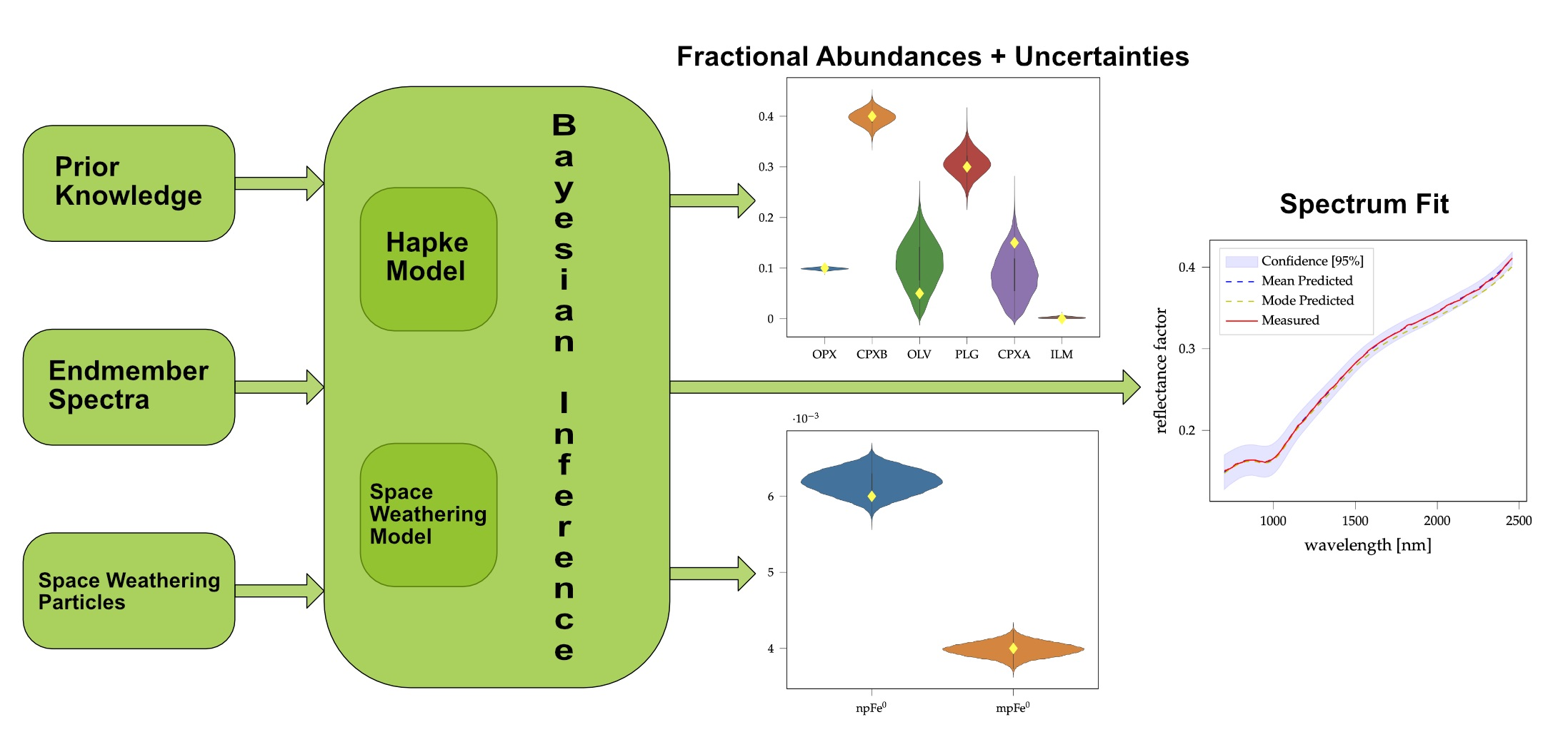
In this work, we develop a Bayesian approach to unmixing. In Bayesian inference (e.g., [23]), all parameters of the model are considered probabilistic variables. In this framework, in addition to the point estimates of the best fit, we also estimate the uncertainties of the parameters. Due to the darkening agents, which darken the spectra and dampen the absorption bands, the uncertainties of the mineral abundances are likely to be higher on the Moon than on other planetary bodies with an atmosphere (e.g., [22]). Additional prior information can be conveniently incorporated in the Bayesian framework. To reduce uncertainties of the mineral abundances, estimates of elemental abundances can be included such that the algorithm will prefer solutions that use endmember combinations with similar elemental compositions.
2. Methods
Generally, the methods employed in this work can be subdivided into two main frameworks. Firstly, the radiative transfer model describes the scattering and absorption behavior of the materials. This framework is built upon the Hapke model [9] and the space weathering model of Wohlfarth et al. [24]. Secondly, the Bayesian framework formalizes the probabilistic perspective of the problem. In the following section, we will describe the choices of the models and their parameters.
2.1. Radiative Transfer Models
2.1.1. Hapke Model
The semi-empirical Hapke model has become the quasi-standard for the analysis of particulate planetary surfaces. Over the years the original model [25] has been refined to also include opposition effects and better approximations for the phase function and Chandrasekhar’s H-function to model multiple scattering inside of the medium. The Modified Isotropic Multiple-Scattering Approximation (MIMSA) formulation of the model [26] is as follows:
The single scattering albedo (SSA) can be calculated by inverting the equation for . The cosines of the incidence () and emittance () angles are denoted as and , respectively. The phase angle g is the angle between the incident and emitted light rays. The phase function is denoted as , the opposition effect is subsumed in the terms for shadow hiding and coherent backscattering . We also include corrections for macroscopic surface roughness as described in Hapke [27], but for the laboratory mixtures used in this work, this effect is not relevant. The multiple scattering term M(,) models the scattering between the particles inside the medium and is described in detail in Hapke [26] and not repeated here.
In general, the phase function p(g) can be represented by a sum of Legendre polynomials weighted with the material-specific Legendre coefficients :
Specifically, the phase function p(g) of the soil can be approximated with the double Heney–Greenstein function [28]:
with the parameter being a measure for the amplitude of the backscattering lobe to the forward scattering lobe. denotes particles that are mainly backscattering. The parameter is a measure of the width of the lobe. For the lunar regolith, Warell [29] found the standard values for the parameter bDHG and cDHG to be 0.21 and 0.7, respectively. According to Yang et al. [30], ilmenite is more back-scattering while the other lunar minerals are mainly forward-scattering. We adopt the parameters for ilmenite from Yang et al. [30] and set bDHG = 0.19 and cDHG = 0.33 for the ilmenite endmembers. For the other endmembers we use the parameters from Warell [29] to be consistent with the previous work of, for example, Rommel et al. [13].
By expanding the Double Heney Greenstein function the Legendre coefficients can be derived from the parameters bDHG and cDHG as follows [26]:
The multiple scattering term in Hapke [26] is derived from the Legendre coefficients of the single scattering phase function p(g). Using only the first 15 coefficients is sufficient, as the decreases with increasing n.
Under small phase angles, the surface appears brighter than would be expected. This is accounted for in the model by the correction terms BSH and BCB, denoting the shadow hiding and coherent backscatter effects, respectively [26]. The samples used in this work were acquired under a phase angle of 30°, therefore, we will assume that the opposition effect is negligible, if not mentioned otherwise.
This model is inverted to find the best fit albedo for the measured reflectance values. This procedure is applied to the endmember spectra that are then used according to the forward mixing model.
2.1.2. Forward Mixing Model
The single scattering albedos of the endmembers obtained by inverting the Hapke MIMSA model are subsequently used to calculate the SSA spectra of the mixture. According to Hapke [9] the single scattering albedo is defined as the scattering coefficients (S) divided by the extinction coefficient (E) of the mixture,
with as the number of particles of particle type i per unit volume and as the cross-sectional area, where denotes the radius of the corresponding particle type [9]. The scattering efficiency is , such that the mixing formula becomes:
The bulk density of particle type i is denoted Mi and the average particle diameter is Di. Assuming that the endmembers have the same average grain size and the same extinction efficiencies , the fraction can be reduced. The albedo of the mixture can then be expressed as a linear superposition of the endmember SSA spectra weighted with the Hapke coefficients ,
For a mixture of typical lunar minerals, the extinction efficiencies, grain size, and density are constant and approximately equal among the endmembers; therefore, these simplifications will be used to calculate the SSA spectrum of the mixed mineral endmembers. This spectrum is then subsequently used as the input to the space weathering framework to calculate the reflectance spectra of the mixture.
When the mixture directly results from the particular known endmembers used in the unmixing, the sum of the weights should be equal to one (). In this work we are not enforcing this constraint, but prefer solutions where the sum is close to one. By not enforcing the sum-to-one constraint for the fractional abundances the sum can be seen as a “catch-all” parameter for all linear, wavelength independent, differences among the endmembers and compared to the examined sample. It is, however, physically implausible to have endmembers with a negative contribution. Therefore, all endmember weights must be larger than zero, that is, .
Apart from the mineral composition and maturity of the sample, other physical properties and the laboratory setups themselves also influence the measured spectra. In this work, we use samples and endmembers of the same grain size fraction to remove the influence of the grain size that has a strong effect on the overall spectra (e.g., [31]). The grain size also introduces large uncertainties for immature spectra [22] and would, therefore, influence the dependencies of the parameters we want to examine in this work.
The porosity or compactness [32] of a sample changes the brightness of a sample almost without introducing a change to the continuum slope. Therefore, this parameter introduces a scaling factor on the weights of the endmembers depending on the compactness of the sample.
Depending on the laboratory setup, other factors might influence the measured spectra. For example, the gain of the sensor might be different such that a linear offset is introduced, when comparing the measurements of the same mineral for different laboratories.
2.1.3. Space Weathering
Space weathering poses a major challenge for unmixing mineral abundances. In addition to the darkening and reddening, the diagnostic absorption features are obscured by the optical influence of the space weathering particles. This makes it harder to differentiate between the different minerals. While the band position remains constant the depth of the absorption that could normally be used to estimate the fraction of the constituent minerals is less clear.
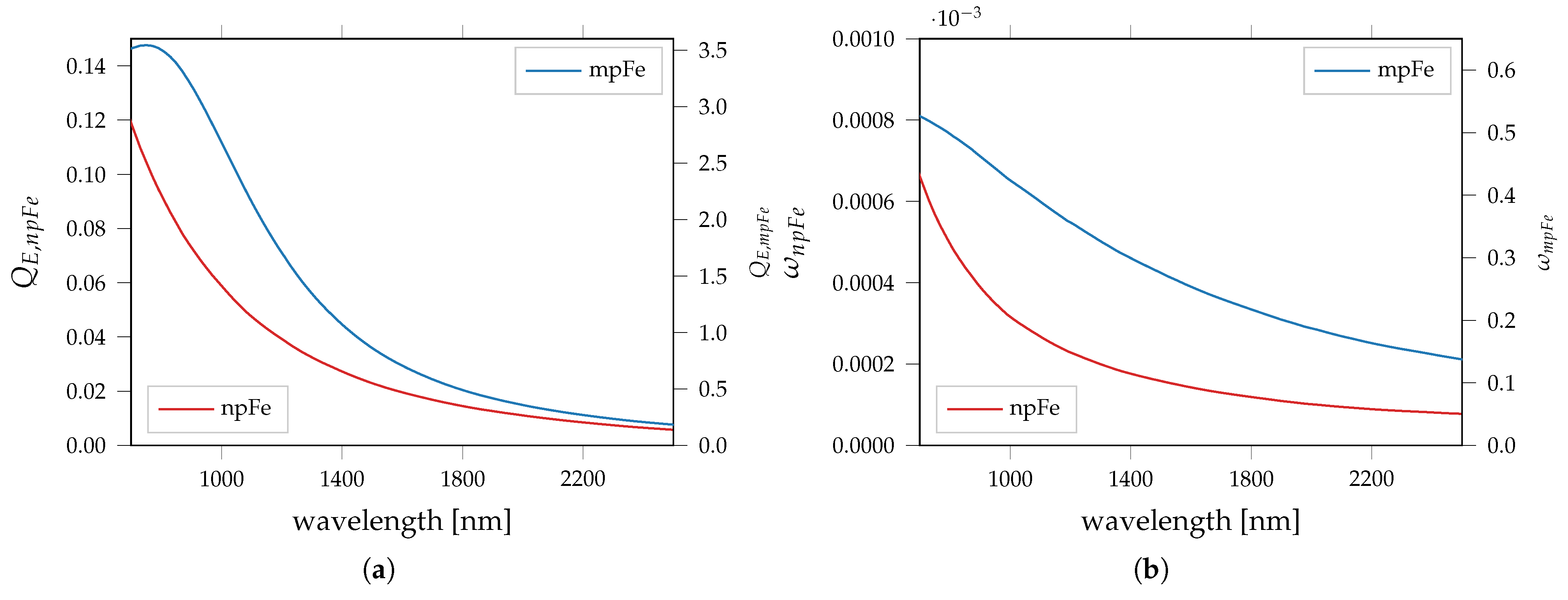
Wohlfarth et al. [24] defined a framework based on ab-initio Mie modeling to characterize the effects of the space weathering particles. We include these characteristics in the unmixing framework. It is important to note that extinction efficiencies are not constant over the wavelength and are very different for the mineral endmembers and for each of the iron particles (see Figure 1a). As a result, the fraction in Equation (7) cannot be reduced. The SSA spectrum of the mixed mineral endmembers () according to Equation (7) is then used as the starting value for the mixture with the iron particles. It is here assumed that all endmembers have a similar grain size distribution, density and extinction efficiencies. The values are adapted from Wohlfarth et al. [24] and listed in Table 1. The mixture of the iron particles and the medium is then defined as:
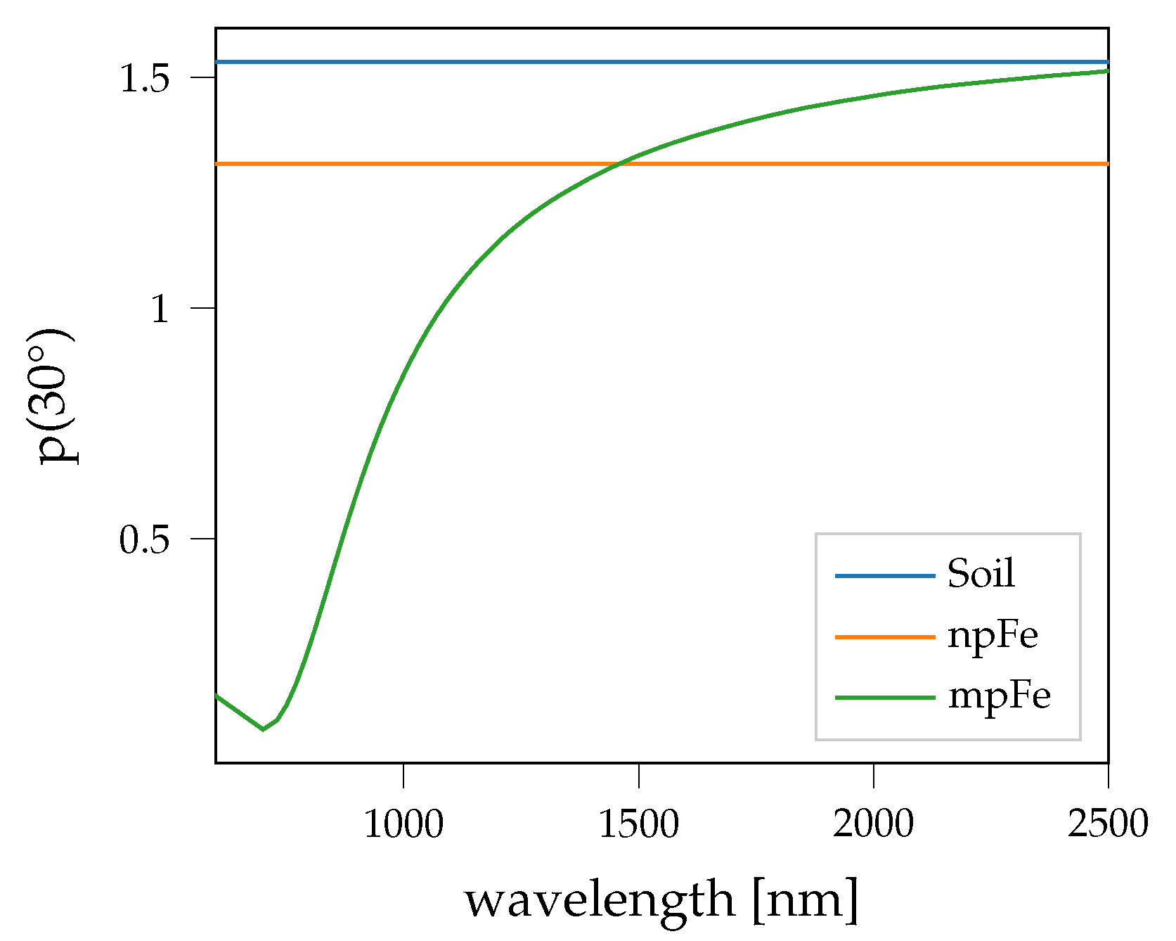
The phase function of a mixture is also defined by the weighted sum of the phase functions of the components. The phase functions of the soil and the small npFe0 particles are independent of wavelength, but the larger mpFe0 particles have a wavelength dependent phase function (see also Figure 2), which is, therefore, given as a vector.
The phase functions are defined by the Legendre coefficients as in Equation (2). These are calculated based on the refractive indices, grain size, and the Legendre expansion of the Mie phase function from Fowler [33]. By equating the coefficients it can be shown that the of the mixture are also the weighted of the soil, npFe0, and mpFe0 particles. The Legendre coefficients of the mixture are then used to calculate the wavelength dependent phase function of the mixture and are additionally used in the multiple scattering term M(). Finally, we obtain reflectance spectra of the mixture, according to Equation (1).
2.1.4. Endmember Catalogs
In order to generate spectra similar to lunar conditions, we need to select endmembers representative of the general mineralogy of the Moon. We are using only mineral endmembers and are not trying to model the influence of agglutinate glasses. This glassy fraction usually has a similar composition to the mineral fraction [34], as it is created endogenously. The absorption band depth is also not affected by glasses, but by a large amount of smFe0 in the agglutinates [35]. Agglutinates here are only relevant for the unmixing of the LSCC catalog in Section 3.3, but this should be kept in mind when evaluating the results.
The highlands are dominated by plagioclase (around 90 wt.%) with the remaining fraction mainly consisting of pyroxenes and minor phases of olivine and spinels [1]. The composition of the maria is more diverse. About 30–40 wt.% are pyroxenes and plagioclase still forms a major part of the composition with up to 60 wt.% of the mineral composition. Olivine contributes up to 10 wt.% and the opaque mineral ilmenite is abundant in some mare areas with up to 20 wt.% at maximum [1].
Among these groups of minerals are also variations depending on the elemental composition. For example, Sun and Lucey [36] showed that by generating albedo spectra based on the magnesium number and grain size the abundance estimation of olivine and pyroxenes can be improved. We will use fixed albedo spectra as endmembers that are chosen to be a good representation of a wide variety of possible true endmembers while retaining the most distinct endmembers.
In general, we want to have one representative of each of the major minerals on the Moon. Pyroxenes can be subdivided into low calcium pyroxenes (LCP), mainly orthopyroxenes (OPX), and high calcium pyroxenes (HCP), usually clinopyroxenes (CPX). The LCP pyroxenes exhibit an absorption 0.9-m and 1.9-m [37,38]. The HCP pyroxenes can be further subdivided into two spectrally distinct groups. Type A, with an absorption at 0.9-m and at 1.15-m, but no absorption around 2-m [37] similar to olivine. Type B, exhibits absorption bands at 1.05-m and 2.35-m [37]. The absorption band positions, however, are not fixed, but vary with Mg2+, Fe2+, and Ca2+ content [39,40]. For the unmixing, the distinction between these three types of pyroxenes (HCP, LCP-A, and LCP-B) is, however, beneficial, because we want to minimize the linear dependencies between the endmember spectra.
2.2. Bayesian Inference
From experience of using unmixing algorithms based on an exhaustive search of all possible endmember combinations (e.g., [13]), we know that several possible combinations can produce similar results. The solution is, therefore, not unique. There might be multiple local minima and some endmembers that are similar, when they become mature, are even gradually interchangeable, without significantly reducing the quality of the fit. Classical unmixing techniques, that are based on finding the best fit in the least squares sense, ignore these uncertainties and only take a single solution, which by a somewhat arbitrary similarity measure best describes the measured spectrum. By exploring the parameter space more thoroughly we can obtain uncertainties and can also learn more about the dependencies among the model parameters.
The process of estimating the probability distributions of parameters of a model based on a set of data and additional assumptions or knowledge about the data is called Bayesian inference (see e.g., [23]). All parameters of the model are described as probability distributions. The goal, therefore, is to estimate the probability densities of the parameters given some data D. This is called the posterior distribution . According to Bayes’ rule the posterior density can be described as:
The data are not changing for one observation, therefore, we can assume that is constant. Consequently, we can define the unnormalized posterior density [23] as:
The probability of the parameters is the prior distribution and can introduce already known information about the distribution of the parameters into the procedure or it can be uninformative. The probability of the data given a set of parameters is denoted as the likelihood (). The likelihood is evaluated as a function of and gives us an estimate on how likely the data have originated from the current parameters.
This unnormalized posterior distribution can be calculated analytically if the probability distributions are chosen in a specific way, which might be limiting in practice. With the advancement of computer technology and the introduction of Markov Chain Monte Carlo (MCMC) methods [41], such as the Metropolis-algorithm [42], it is possible to estimate complex probability distributions numerically. The algorithm used in this work to sample from the posterior density distribution is described in the following section.
2.2.1. Sampling Algorithm
The goal of the Monte Carlo simulation is to approximate the posterior distribution. Most of the sampling algorithms as well as our approach are based on the Metropolis algorithm [42], which was subsequently generalized to non-symmetrical proposal distributions and is then called Metropolis–Hastings algorithm [43]. This algorithm describes a random walk through the posterior space such that for a large number of samples, the samples converge to the posterior distribution. Generally, at each step of the Markov Chain a proposal ) is randomly generated based on the current location in parameter space. This proposal is then either accepted or rejected and the current parameters are consequently used for the next proposal. If the proposal is more probable than the current sample, then the proposal is always accepted; if the proposal is less likely than the current sample, it is accepted with a certain probability. Therefore, less probable solutions are also sometimes accepted.
The random walk behavior of the Metropolis algorithm can, however, lead to slow convergence because many proposals are rejected (e.g., [23]) and correlated parameters can make the algorithm much less efficient [44]. Modified versions of the Metropolis algorithm improve the proposals by, for example, estimating the covariance matrix on the previous examples and scaling the proposal distribution accordingly (e.g., [45]) or by additionally proposing an alternative step that is chosen based on the rejection of the first proposal [46]. However, it still remains that these methods tend to be less efficient for non-linearly correlated parameters, due to their inherent random walk behavior [44].
Hamiltonian Monte Carlo (HMC) borrows ideas from Hamiltonian dynamics [47] and introduces a ’momentum’ variable. As in Hamiltonian dynamics, the momentum variable and the position are building a dynamic system. The entire sampling process is subdivided into simulations of L leapfrog steps each of length . To calculate the momentum at a position in posterior space we need to calculate the derivative of the posterior density for the local environment. With the advances in automatic differentiation in tools like, for example, Theano [48], which is used in the pymc3 framework [49], it is possible to quickly calculate the derivatives of more complex functions.
The two parameters of HMC (L and ), however, must be tuned by hand and strongly influence the performance of the algorithm. The parameter L determines the length of one simulation of Hamiltonian dynamics and, if chosen too large, the leapfrog steps tend to do a U-turn and return to the starting location [23]. The No U-Turn Sampler (NUTS) [44] is an extension to HMC that automatically stops one simulation of Hamiltonian dynamics when the leapfrog step would not increase the distance to the starting location and, therefore, removes the need to tune the L parameter by hand [44]. This way, the NUTS sampler can effectively explore the posterior space.
This algorithm is likely the best choice for our problem, because we can effectively sample from a posterior distribution where we expect some parameters to be correlated and the target distribution might be multimodal.
2.2.2. Likelihood
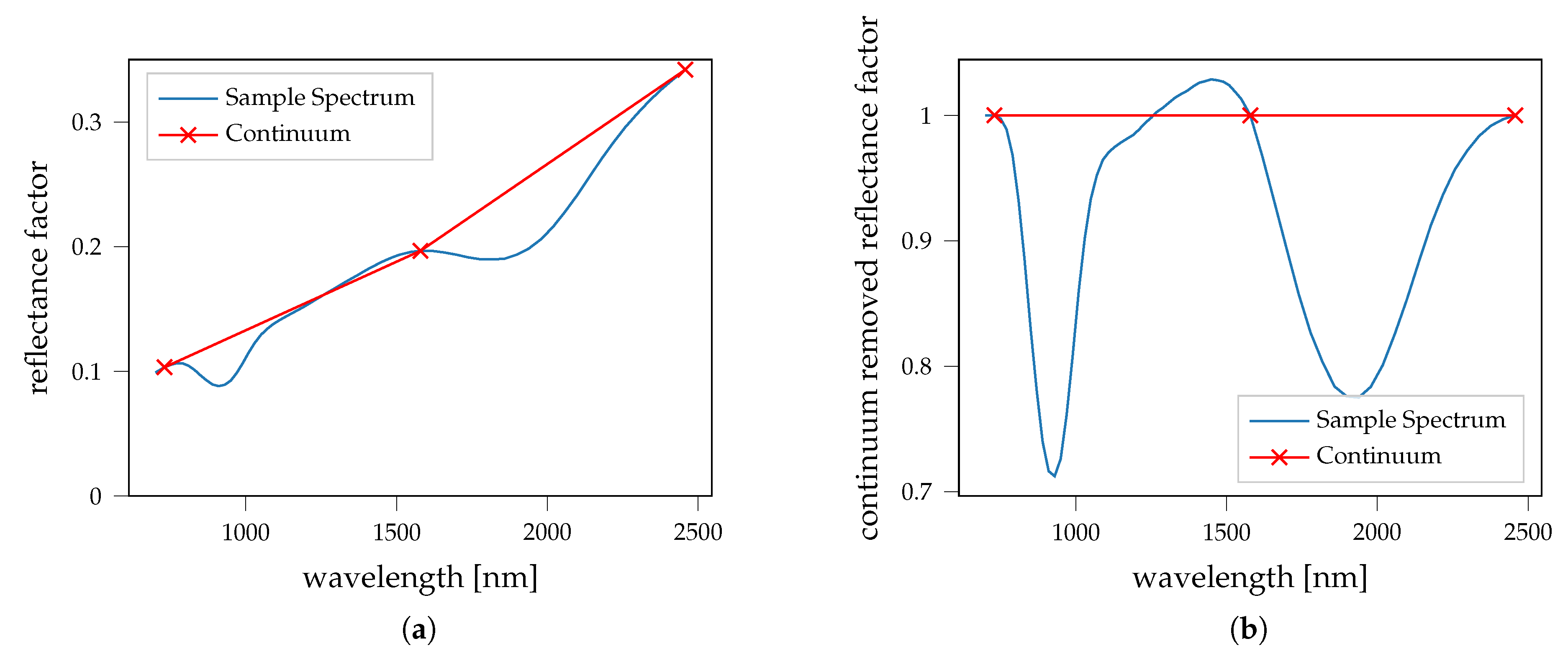
The unmixing problem according to Section 2.1 is that the abundances () of the endmembers and the space weathering components npFe0 and mpFe0 () with known albedo spectra, extinction efficiencies and phase functions must be determined. They are the parameters we estimate with the help of MCMC. The known data that is used to calculate the reflectance spectra are denoted as . The likelihood/goodness of fit of the current parameter estimates is evaluated with both the reflectance spectrum () and the continuum removed spectrum () to emphasize the absorption band depths over the absolute fit. The continuum removed spectrum is calculated in a straightforward way such that certain fixed wavelengths are chosen as the points of the continuum (see, Figure 3). Usually, the continuum is defined by the convex hull of the spectrum (e.g., [50]). Calculating the continuum in this way is very time consuming considering that the function and its derivative must be evaluated thousands of times. The convex hull is not a linear function such that it is inefficient to implement it in Theano because the derivatives cannot be determined easily. The indices of the local maxima would be dependent on the current spectrum. Because for each of the current parameters of the Markov Chain the continuum is different and depends on the slope, it cannot be computed prior to the sampling. Both the method using the convex hull and the method using fixed wavelengths used in this work are able to characterize the absorption bands usually found on the Moon.
Therefore, the concatenation of the spectrum and the continuum removed spectrum represents the data S. The output of the model is, therefore, a function of the parameters and such that:
The likelihood is then evaluated by building the sum over all log likelihoods or the product of all probability density function values at the measured data (), given a normal distribution around the modeled data and some variance , which is also considered a parameter of the model and, therefore, is also sampled.
K denotes the number of channels. If we know that the model’s accuracy is wavelength dependent, it is reasonable to include this information in the likelihood function. Therefore, we introduce a wavelength dependent scaling factor () that can be used to emphasize, or de-emphasize certain wavelength channels.
2.2.3. Prior
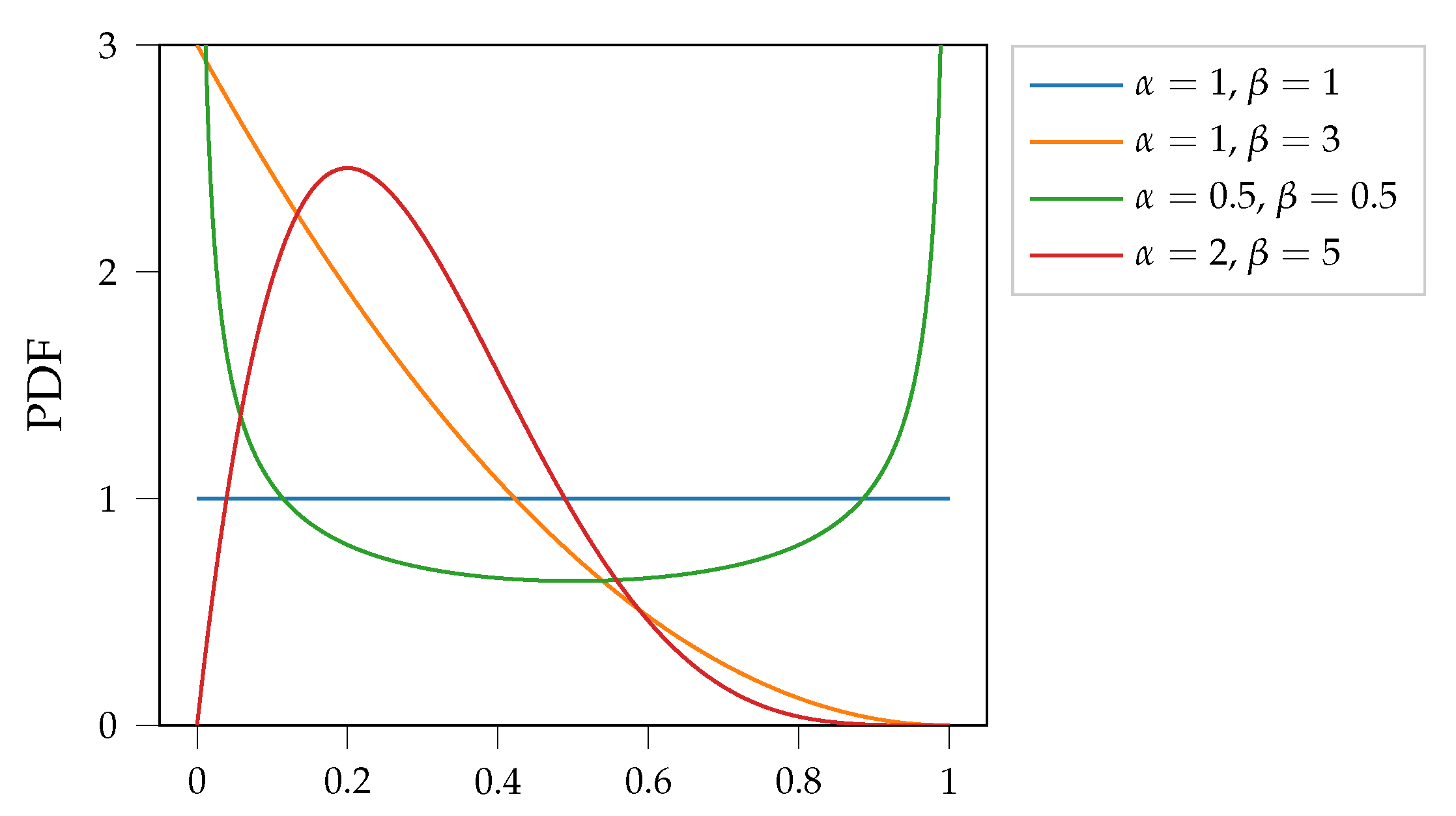
Bayesian inference offers a convenient way to include a-priori knowledge in the sampling process. As described in Equation (11), the posterior is proportional to the likelihood and the prior . For multiple priors, the joint probability is given by the product of the individual probability. Because our parameters are usually limited to the interval of [0, 1], a good choice for the priors on our parameters is the Beta distribution, which is defined by two shape parameters and as follows [51]:
with denoting the gamma-function. Choosing and controls the shape of the Beta distribution. Some examples are shown in Figure 4. For example, for a distribution with and , the mode of the distribution is 0.2, but for a distribution with and , the mode is zero and the probability decreases for increasing values. For values outside the interval [0, 1], the probability is zero.
The prior distribution on the endmember abundances can be set as follows, with the shape parameters being chosen depending on the application:
The space weathering components, namely npFe0 and mpFe0, form only a small fraction of the composition. Therefore, we can choose the prior similar to and in Figure 4 for each abundance of npFe0 and mpFe0 ()
The shape parameters will be chosen such that small values are preferred by the sampler.
We do not enforce the sum to one constraint to account for differences in the laboratory setups of the endmembers as well as porosity and other influences. Nonetheless, it is sensible to set a prior on the sum of the endmember weights :
This prior is centered around one such that solutions where the sum of the endmembers is close to one are favored. The variance is chosen depending on the differences among the endmembers and the investigated samples.
The elemental abundances can be relatively well characterized remotely with, for example, gamma ray spectroscopy (e.g., [52]). Spectral parameters in the UV (e.g., [3,4]) or in the NIR (e.g., [5]) can also be used to estimate the elemental abundances, but should be used with care. For example, according to the TiO2 maps of Sato et al. [4] the swirl Reiner Gamma is deprived of TiO2 compared to its surroundings, which is physically implausible, as the optical differences are likely due to a difference in maturity and/or compaction [53]. Setting a prior, however, does not rule out solutions that do not confirm with prior knowledge, as long as the probability of the prior does not become zero. If, for example, the spectrum fits better for a high ilmenite concentration, this solution will be found to be more likely.
The RELAB database provides elemental abundances for many of the samples (e.g., [37]) and the elemental composition of the endmembers from Rommel et al. [13] were determined by electron microprobe analysis. We here use endmembers with well-defined elemental abundances (, matrix, for M elemental abundances and N endmembers) and use the estimated elemental abundances of the samples (, ) as prior information. If the samples are mixed directly from the endmembers with weights () the actual elemental abundances can be calculated as
For realistic mixtures, this relationship produces highly non-unique solutions for the mineral weights because, for example, the MgO abundance could be attributed to a pyroxene or an olivine. For each sample the elemental abundances are calculated based on the proposed parameters of the mineral abundances according to:
As the beta distribution should be centered around the estimated elemental abundance we want to enforce the mode of that distribution to be equal to the estimated elemental abundance. The mode of the Beta distribution for and is given by:
By increasing (), the variance of the distribution decreases. Therefore, we choose a approximately according to the desired variance of that particular element and calculate according to Equation (20) such that:
Consequently, we define the prior for the elemental abundances to be:
This distribution then effectively acts as a prior on the weights of the mineral endmembers, but there are multiple combinations that fit equally well.
3. Results
The measured spectrum of a mixture is influenced by several factors, namely (1) composition (2), space weathering, (3) grain size, and (4) porosity. To disentangle the effects, we designed several experiments. The grain size is constant for all experiments and is expected to be known. Firstly, we calculate mature synthetic spectra to remove effects not described by the mixing model itself, except for noise. This can also be interpreted as a general validation of the sampling approach. Secondly, to remove the influence of space weathering and to test the general viability of the mixing model we used laboratory mixtures of known endmember spectra. Thirdly, we apply the full framework to unmix the LSCC spectra with endmember spectra from the RELAB catalog and include space weathering particles. These LSCC spectra can be seen as a good representation of different maturity levels and the general mineralogy of the lunar maria.
3.1. Synthetic Mixtures
This experiment is designed to estimate the uncertainties of the mixtures when all influences not covered by the model are removed. Spectra are generated with the mixing model including additional Gaussian noise with a standard deviation of . This corresponds to a signal-to-noise ratio (SNR) between approximately 170 and 400 (with SNR ) depending on the channel.
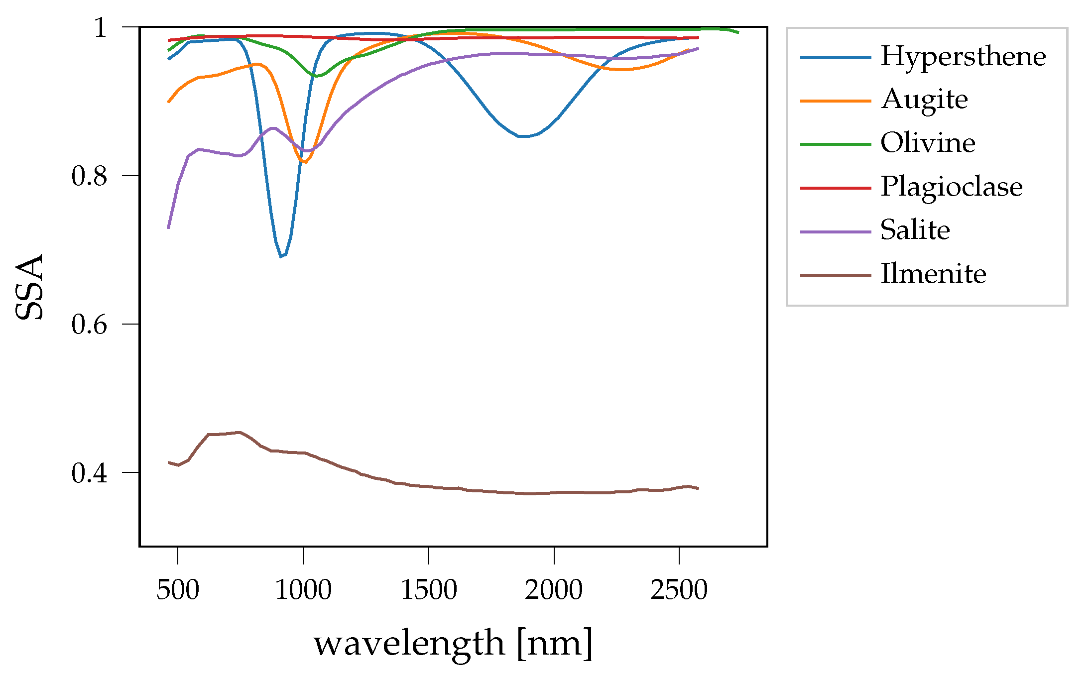
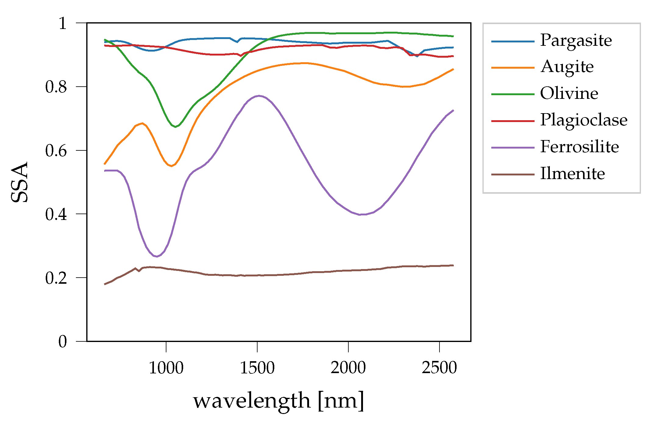
We selected the endmembers according to the categorizations above (see Section 2.1.4). A representative of each of the classes LCP, HCP Type A, HCP Type B, Olivine, Plagioclase, and Ilmenite is selected from the RELAB catalog (https://pds-geosciences.wustl.edu/spectrallibrary/default.htm, accessed on 1 November 2020) and the SSA values are obtained by inverting the Hapke model and displayed in Figure 5. All endmembers are samples of the 0–45 m size fraction. The elemental abundances of the endmembers are listed in Table A1.
The generated mixtures are based on a mare composition of the endmembers of 10 wt.% hypersthene, 40 wt.% augite, 5 wt.% olivine, 30 wt.% plagioclase, and 15 wt.% diopside. The ilmenite abundance is varied between 0 wt.% and 16 wt.% and the remaining fraction is normalized, such that the endmember weights again sum up to unity. The abundances of npFe0 and mpFe0 is varied between 0 wt.% and 2.2 wt.%, and 0 wt.% and 1.2 wt.%, respectively. Ultimately, 48 synthetic mixtures (mix0–mix47) are created. The detailed results for all mixtures are listed in Table A3 and Table A4.
Generally, all endmembers are measured under similar conditions. According to these conditions the priors have to be chosen. In our case, we do not want to directly employ knowledge about mineral abundances (). Therefore, we choose an uninformative prior, that is:
Both shape parameters of the Beta distribution are set to one for the prior distribution, such that the prior is a uniform distribution between zero and one. Because negative weights are physically implausible, these samples are always rejected.
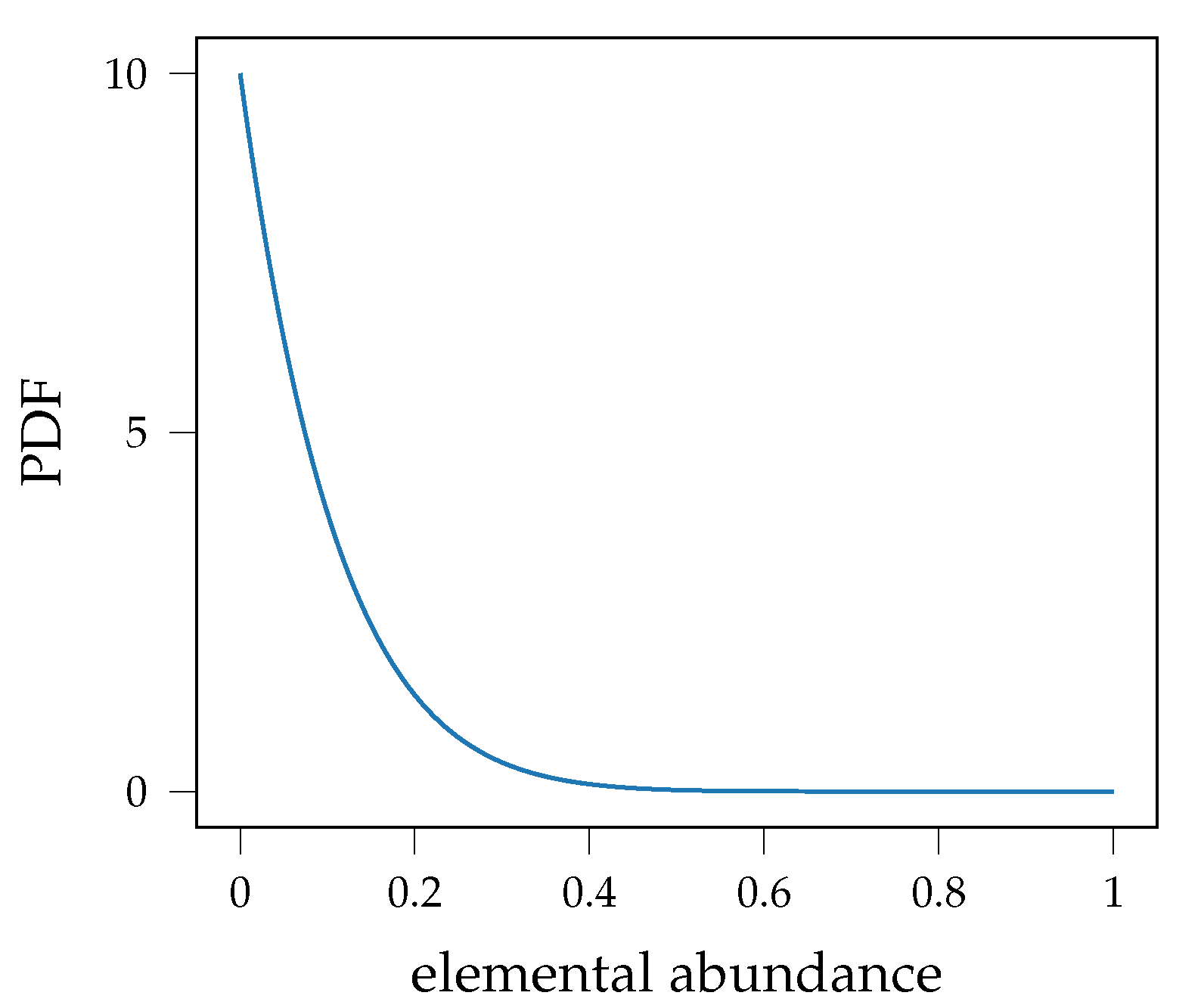
The mixtures are synthetically generated, such that we set to prefer solutions where the sum of the fractional abundances is close to one. The experiment is carried out once with no prior on the elemental abundances and once with an elemental prior on the abundances of TiO2 and Al2O3 (see also Table 2). For theoretical abundances below 1 wt.% the variance becomes very low when using the method mentioned above. Therefore, we set and for the shape of the prior, making the mode zero and the PDF is given in Figure 6.
In general, we set the shape parameters for npFe0 and mpFe0 to and . These parameters were tuned by hand such that 80% of the probability density is distributed in the interval [0 wt.%, 5 wt.%]. Higher values than 5% are physically implausible. Trang and Lucey [54] found about 2 wt.% of smFe at the maximum for the Moon, excluding the polar regions. The model of Trang and Lucey [54], first versions of which were introduced in Trang et al. [55] and Lucey and Riner [16], differs from the model of Wohlfarth et al. [24], for example, Trang et al. [55] do not consider the influence of the phase function. Therefore, the predicted concentration of npFe0 and mpFe0 is not necessarily the same, leading us to set a relatively uninformative prior on each of the smFe abundances. The prior on the abundance of smFe particles is consistent throughout this work and is not changed between experiments.
Generally, the mean predicted solution does not necessarily correspond to the actual mixture coefficients used, but the theoretical values are always part of the solution. Classical unmixing approaches are limited to just one solution and small changes may lead to different optimal solutions, which are also not necessarily equal to the ground truth values.
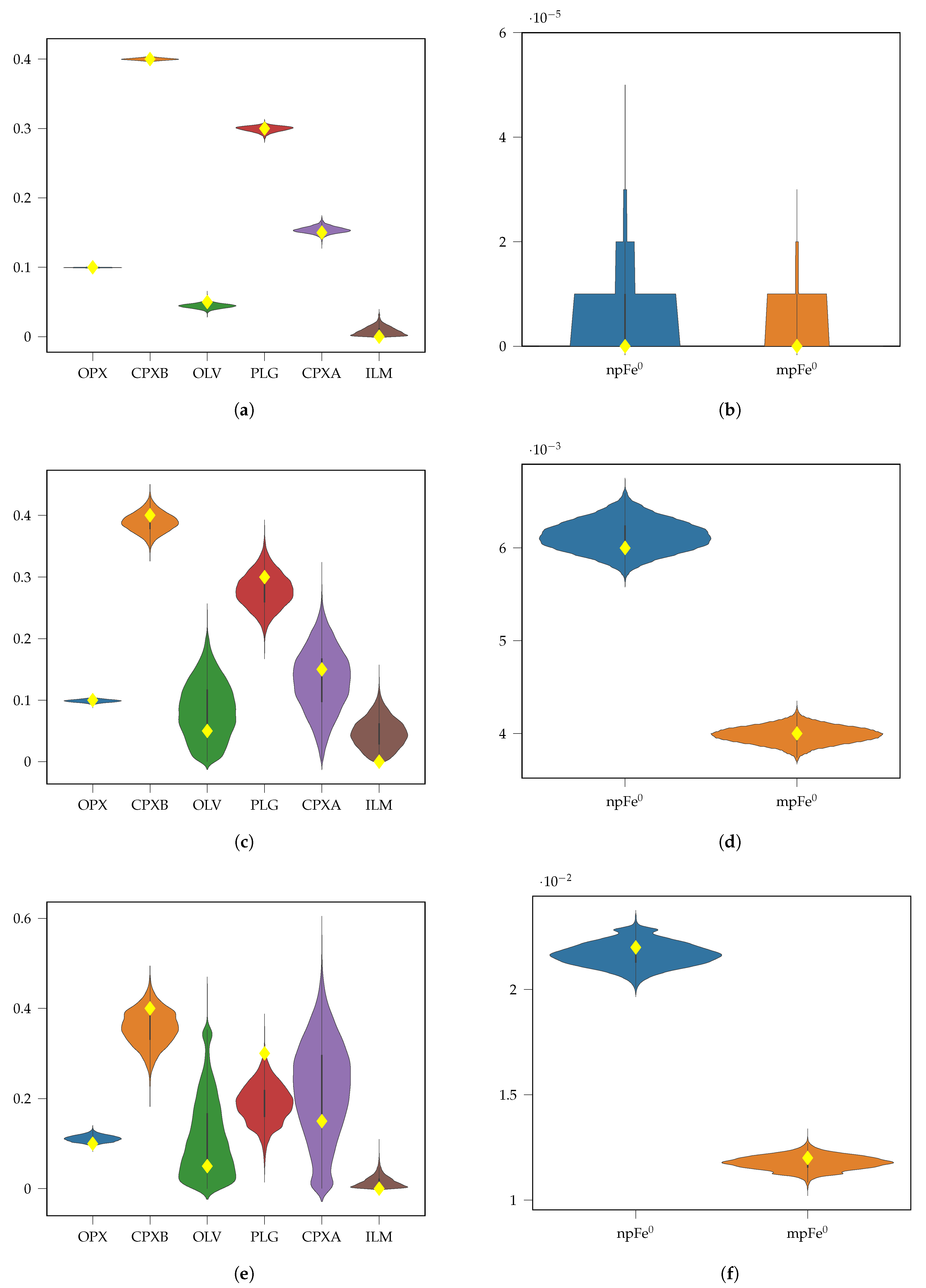
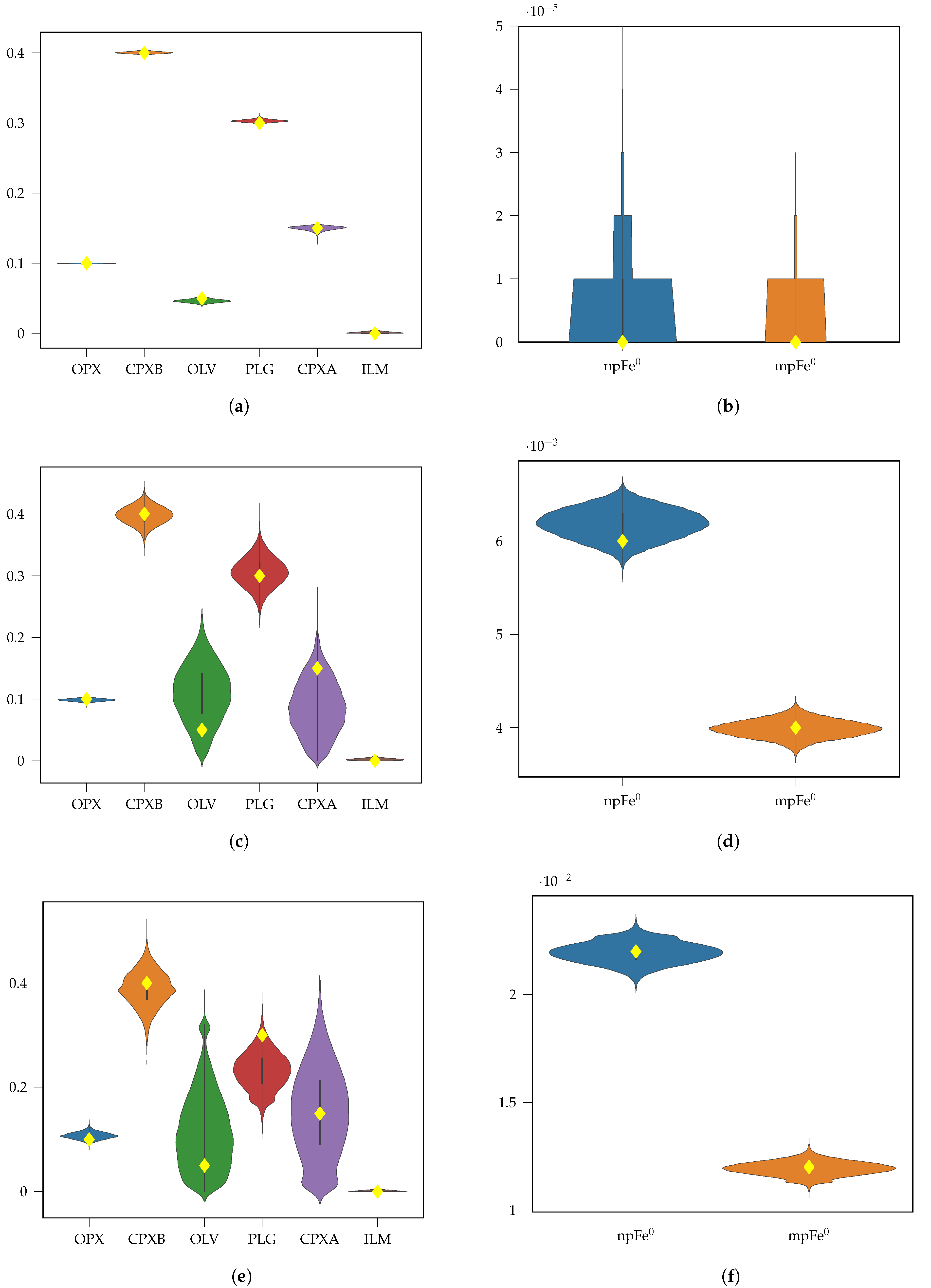
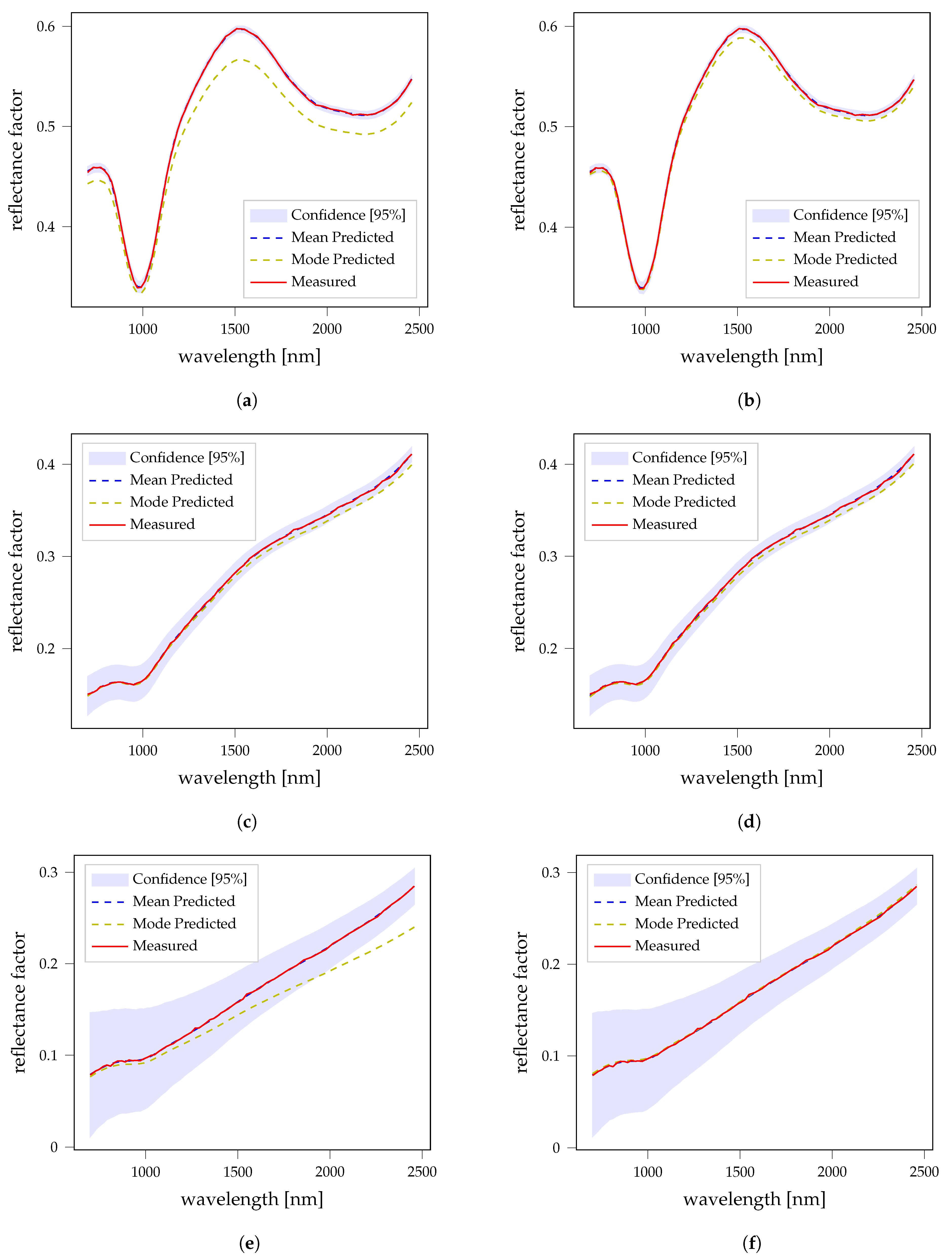
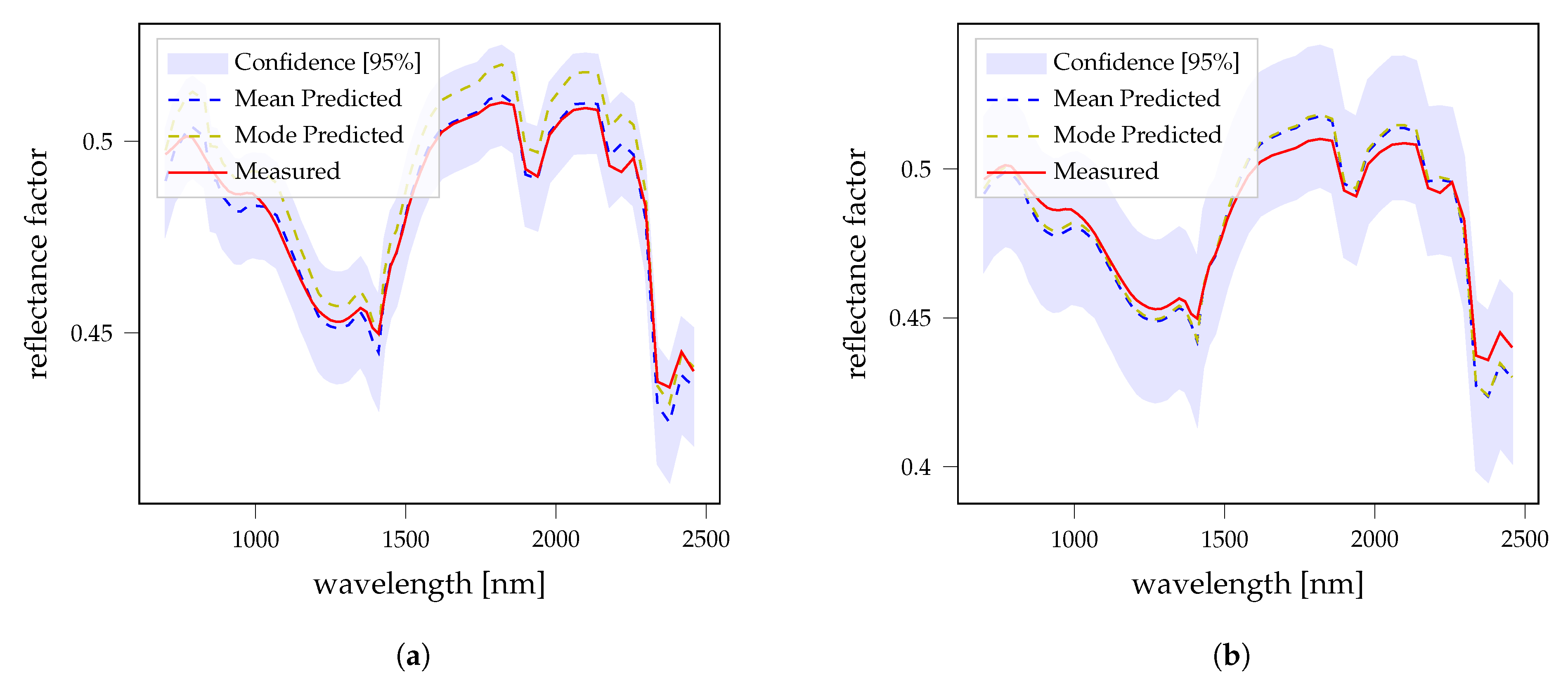
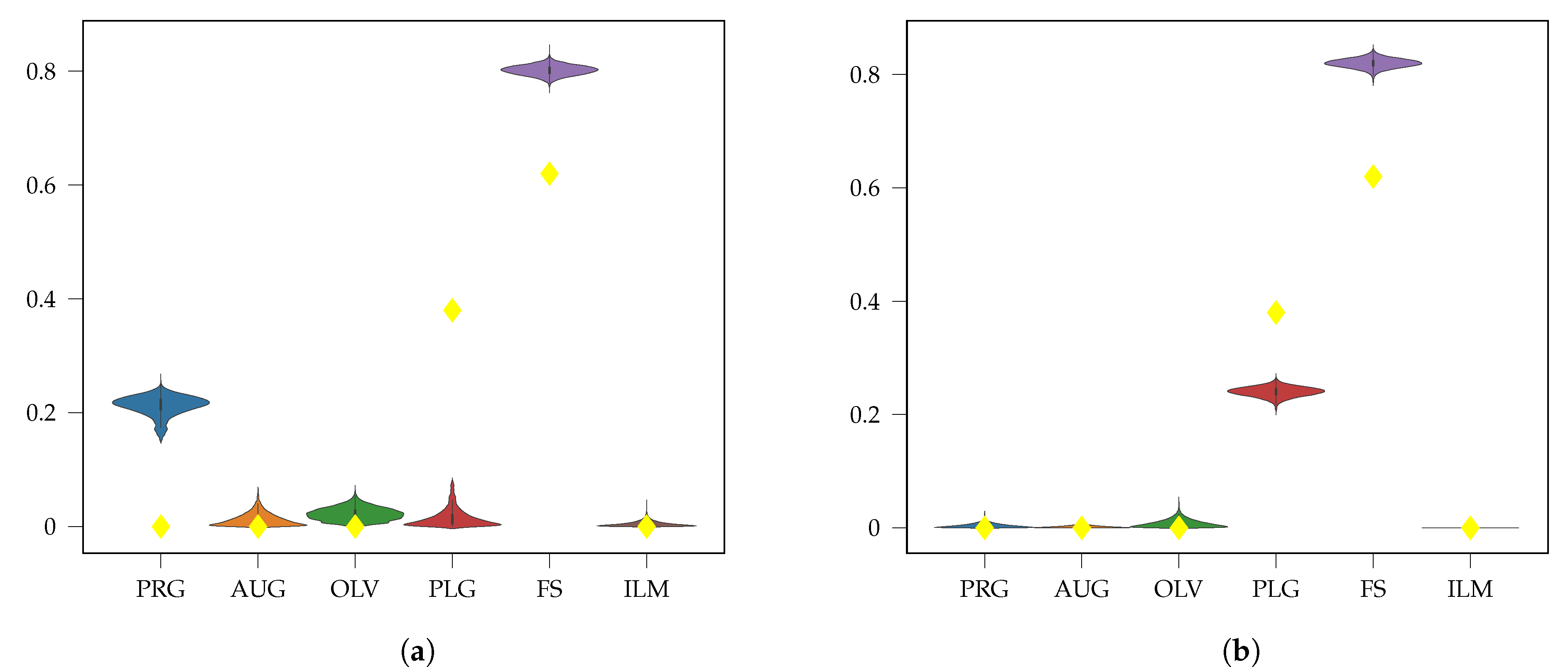
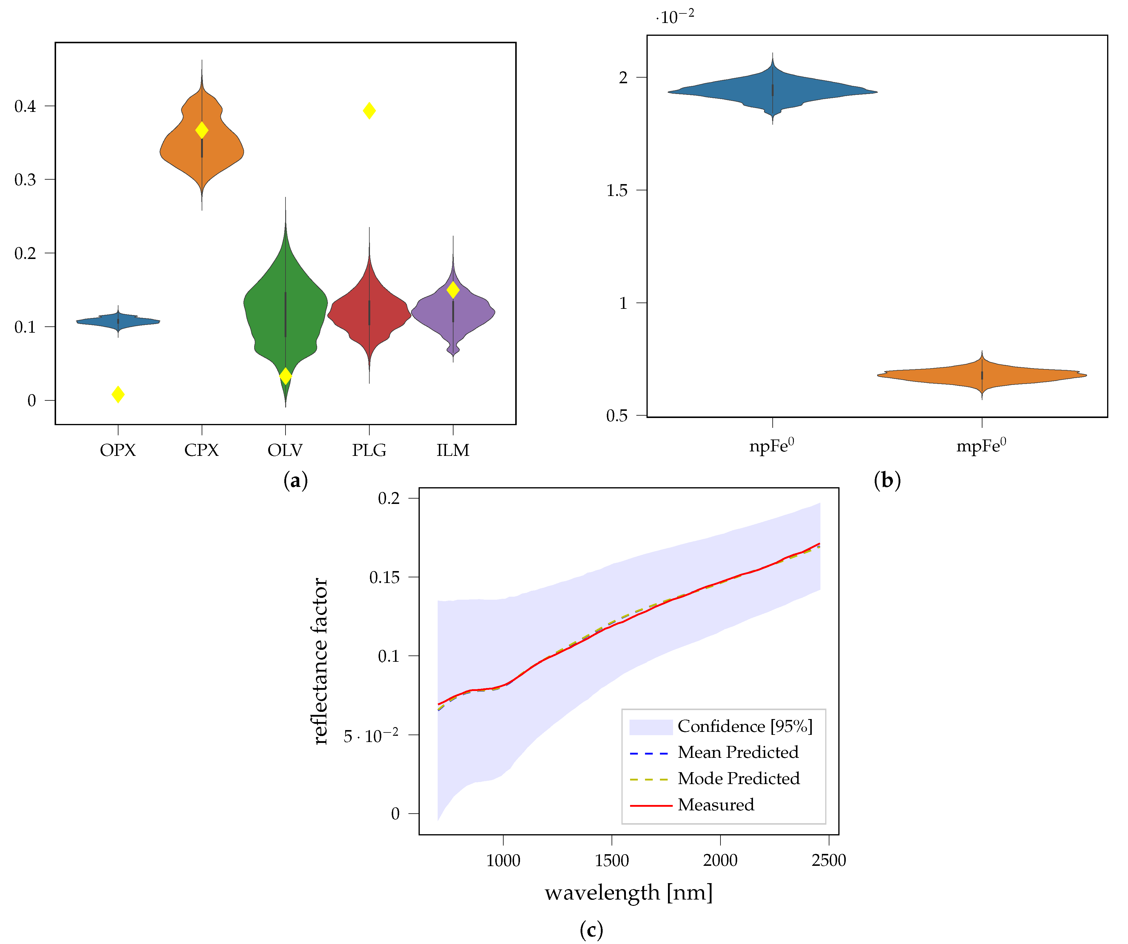
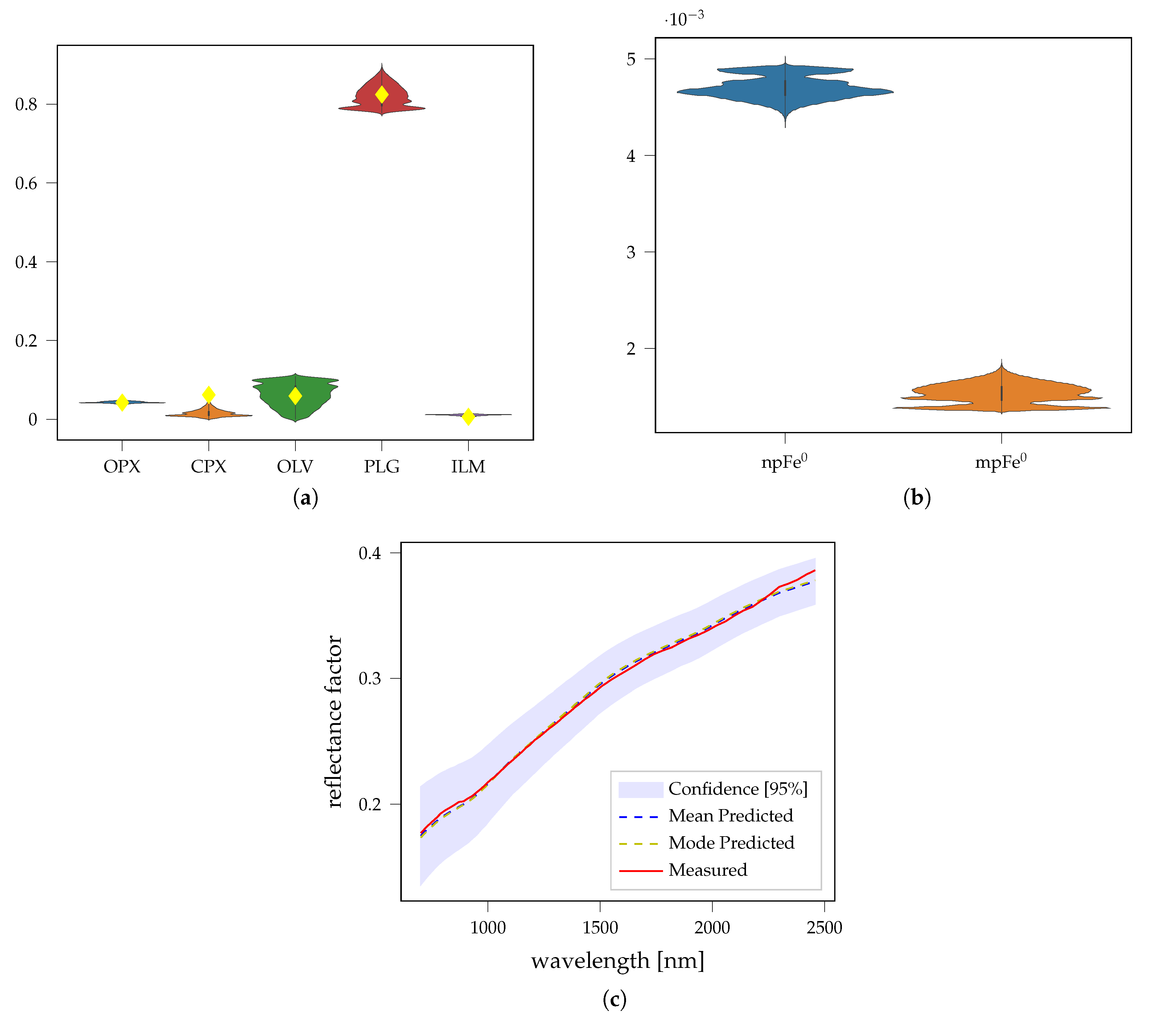
Ilmenite shows, compared to the mafic minerals, an almost featureless spectrum in the NIR wavelength range. Because of its low albedo, the abundance of ilmenite also dampens the absorption bands and darkens the overall spectrum. This is, to some extent, similar to the spectral influence of mpFe0 particles. If the absolute reflectance is poorly defined, so is the ilmenite abundance. Consequently, depending on the prior setup and the sum constraint the uncertainties of ilmenite are different. If no prior on the elemental or mineral abundances is set, the abundance of ilmenite is relatively poorly defined. For the mixtures that, in theory, do not contain ilmenite, a majority of the accepted mixtures contain significant amounts of ilmenite (see Figure 7). A combination of ilmenite and other endmembers can, therefore, equally explain the measured spectrum. This effect can be mitigated when a prior is used (see Figure 8). For the fresh mixture (mix0), without any smFe particles, the uncertainty of the spectrum is small (see Figure 9). The mineral uncertainties are small, but for the other mixtures, the uncertainties significantly increase. The majority of posterior density of plagioclase (PLG) is generally lower than the actual abundance, and for olivine (OLV) and/or diopside (CPXA) the majority of posterior density is below the actual value. This suggests that a mixture of olivine/diopside and ilmenite produces very similar results to plagioclase. Olivine and diopside have similar absorptions at about 1-m, making them interchangeable to some extent when the maturity increases. For example, for mix15 there are two distinct modes with either high concentration of diopside or olivine. The mineral uncertainties of mix5 are large, but the spectrum is clearly defined. This highlights that there are several solutions that produce nearly identical spectra. Sometimes, however, the modal abundance values do not sum up to one, because, for example, just one of the distributions is skewed. This can lead to mode predicted spectra outside of the confidence band. The modal abundance values were likely never sampled in this particular combination.
Ilmenite is the only endmember that contains significant amounts of TiO2. Including prior knowledge about the abundance of TiO2 can, therefore, favor solutions that are close to the true ilmenite value. In Figure 8 the violin plots of the acceptable solutions considering the TiO2 and Al2O3 prior are displayed. The abundance of ilmenite is then much more clearly defined. The uncertainties of the other minerals also mostly decrease, while the uncertainties of the spectra remain similar.
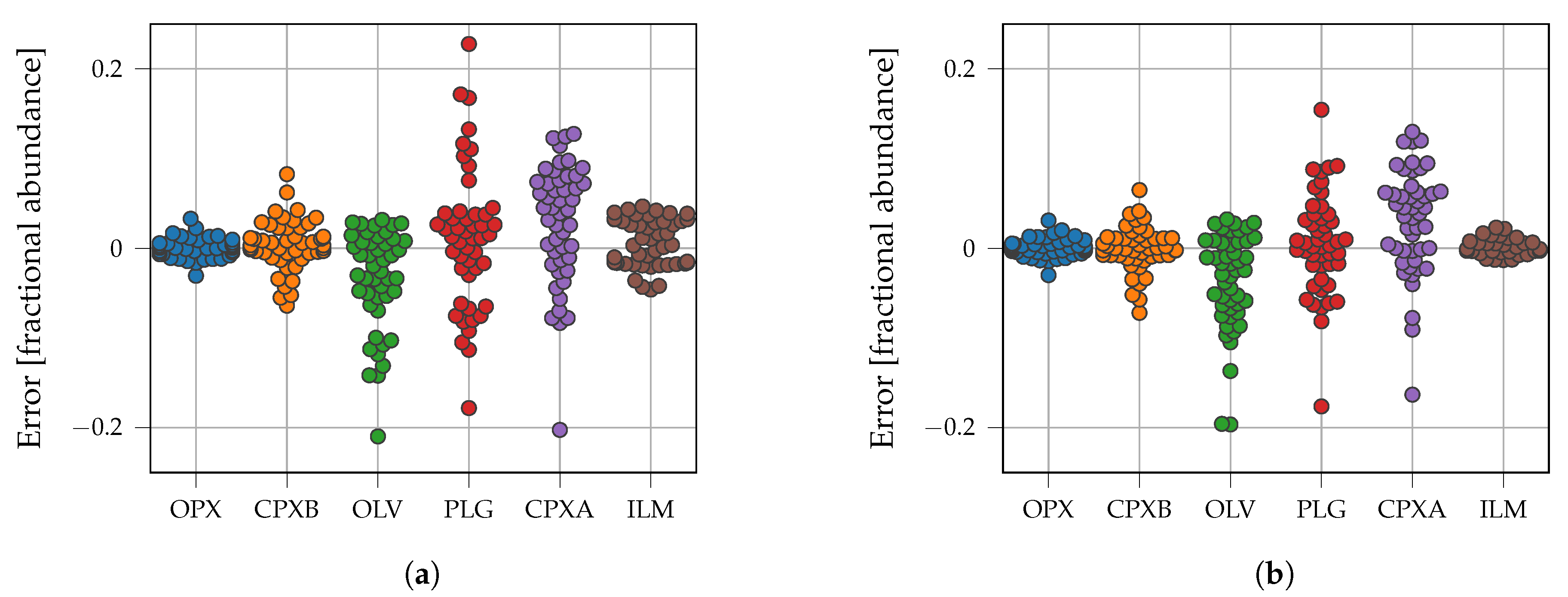
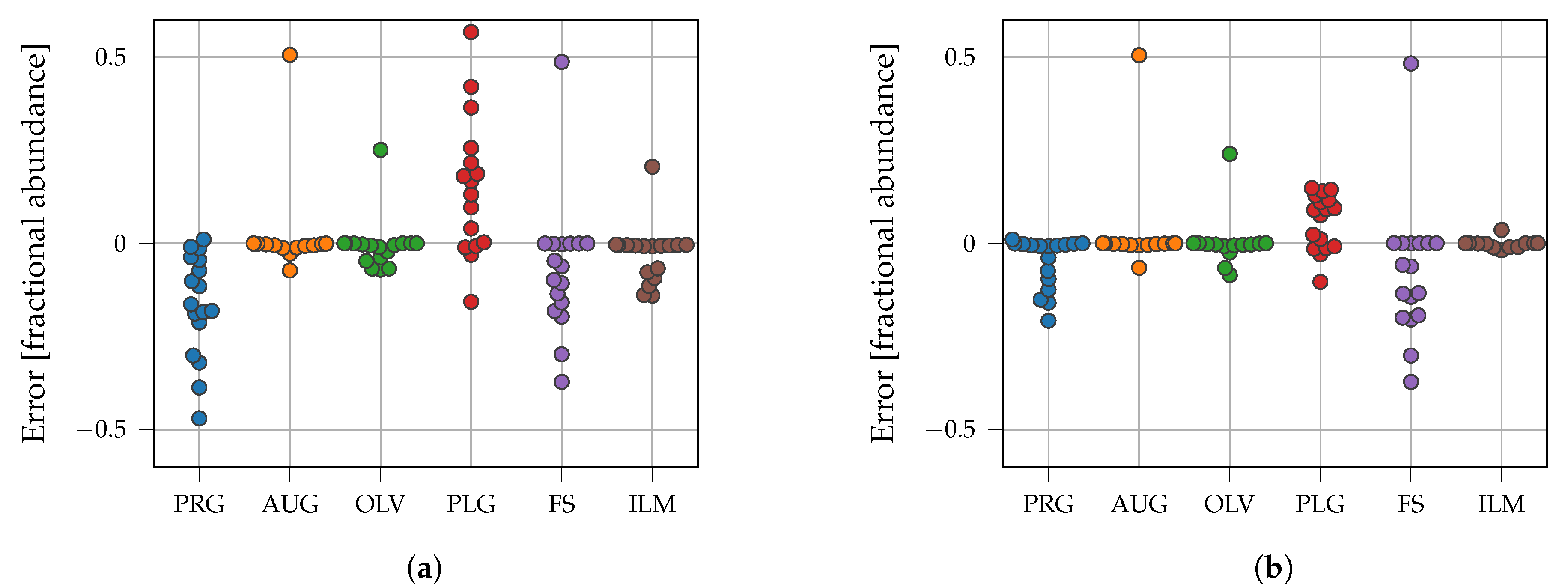
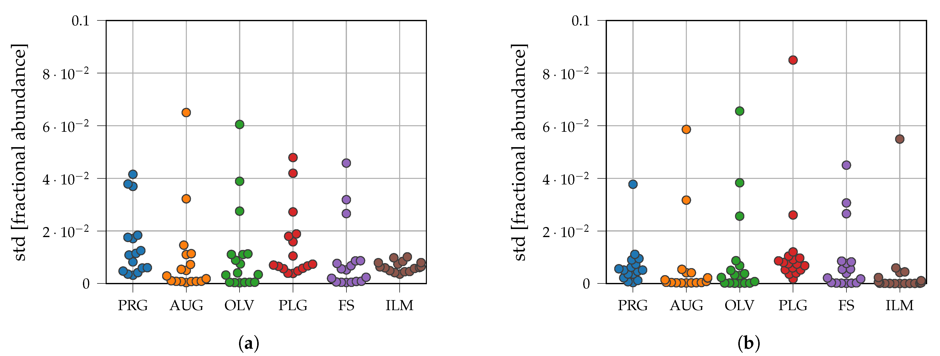
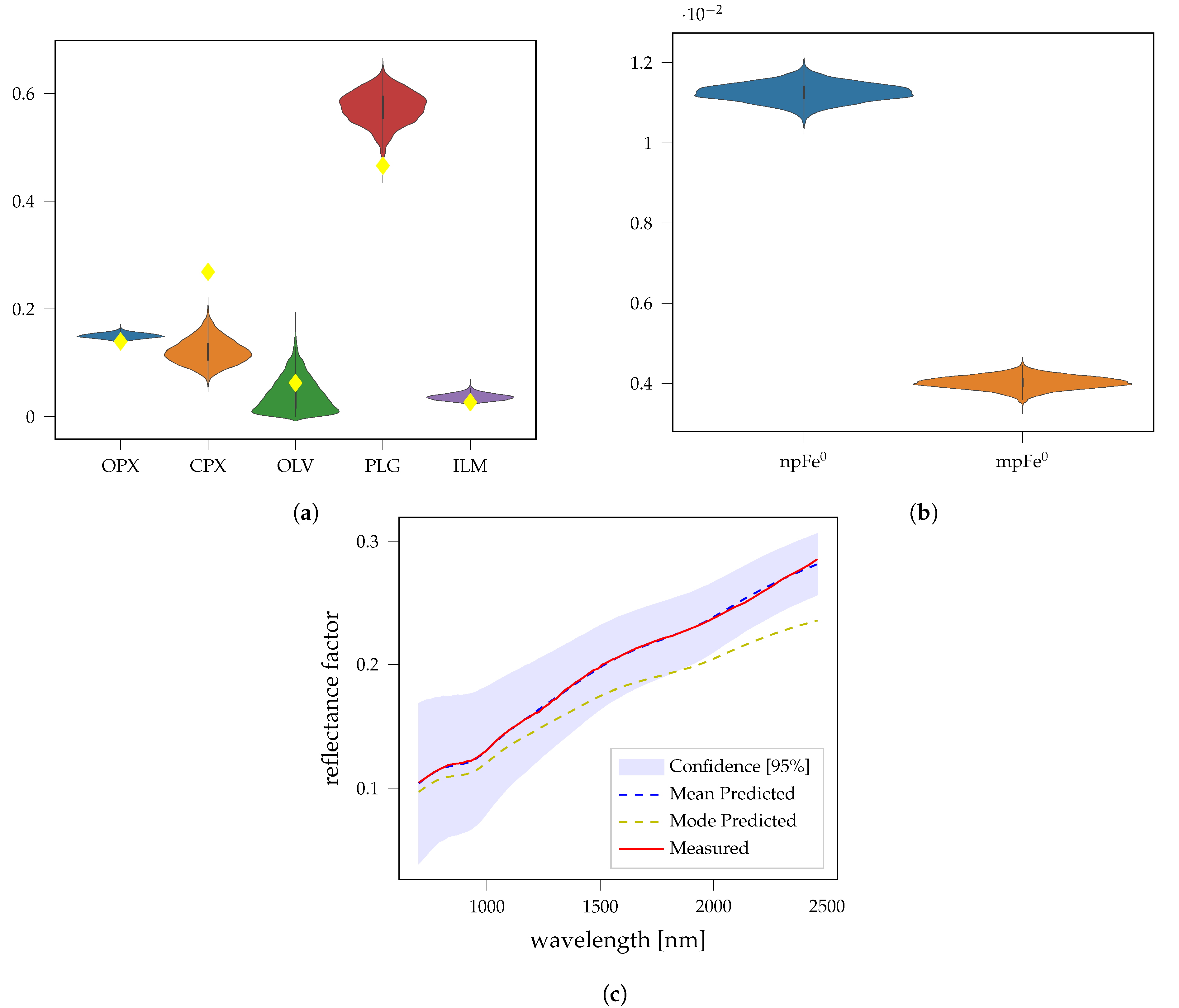
The results for the most mature spectrum with the highest abundance of ilmenite are shown in Figure 10. With the prior, the uncertainties of all endmembers can be reduced. The confidence plots remain very similar. Figure 11 shows the distribution of the differences between theoretical values and mean predicted abundance. By including the prior the differences can be reduced. The mean of olivine is usually above the true value, while the mean of plagioclase and clinopyroxene is usually below the theoretical value. The theoretical abundance of olivine is relatively small compared to the other minerals, consequently, the mean is usually higher. The uncertainties of olivine and clinopyroxenes are high for both with and without the prior. This can be seen in Figure 12. Including prior knowledge about the elements Al2O3 and TiO2 the uncertainties of all mineral abundances are mitigated. This is despite the fact that these elements are almost depleted in the pyroxenes and olivine.
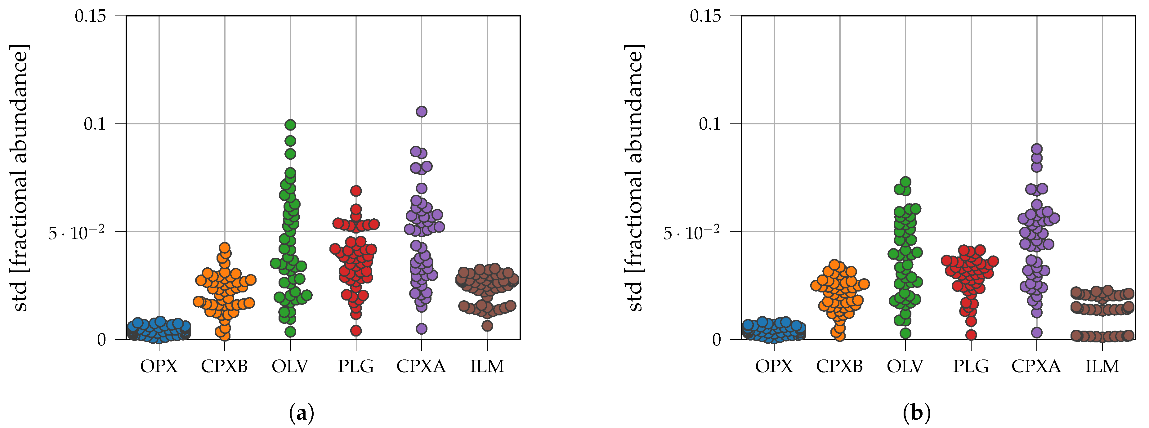
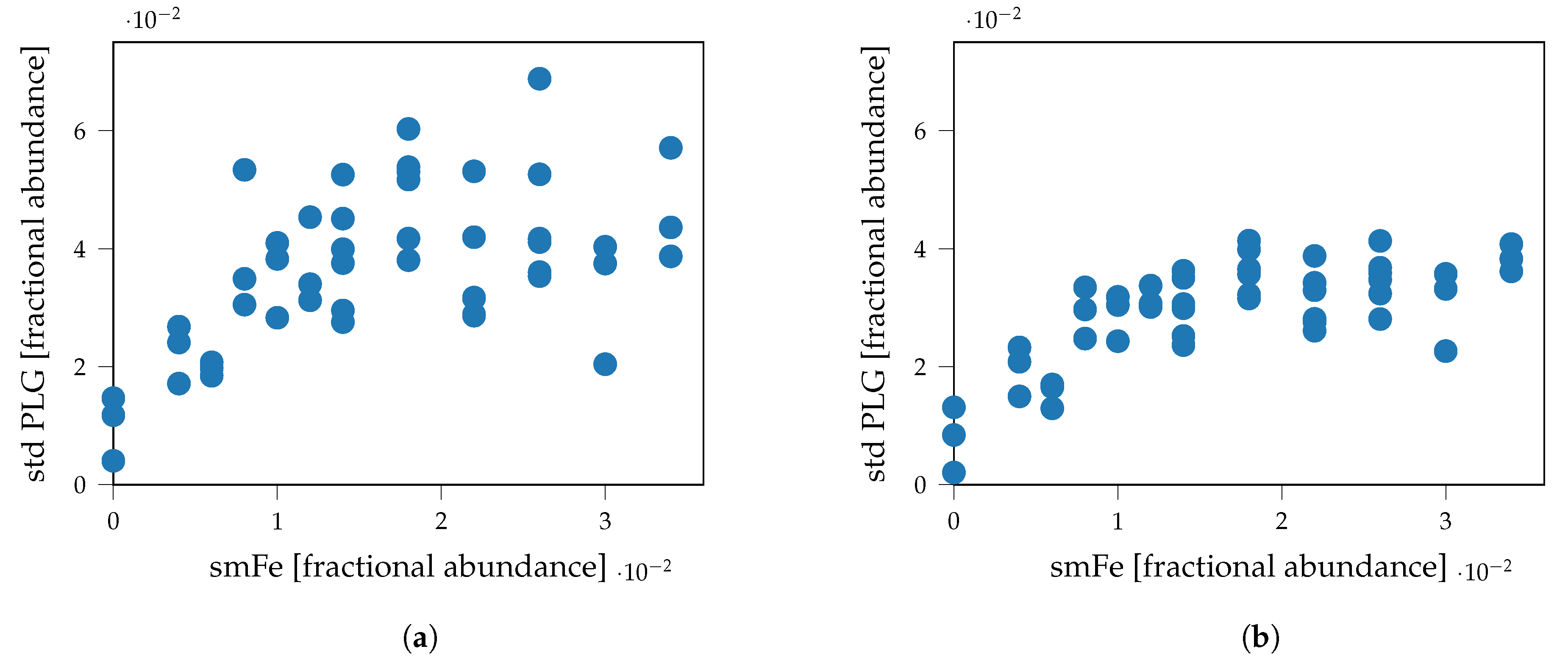
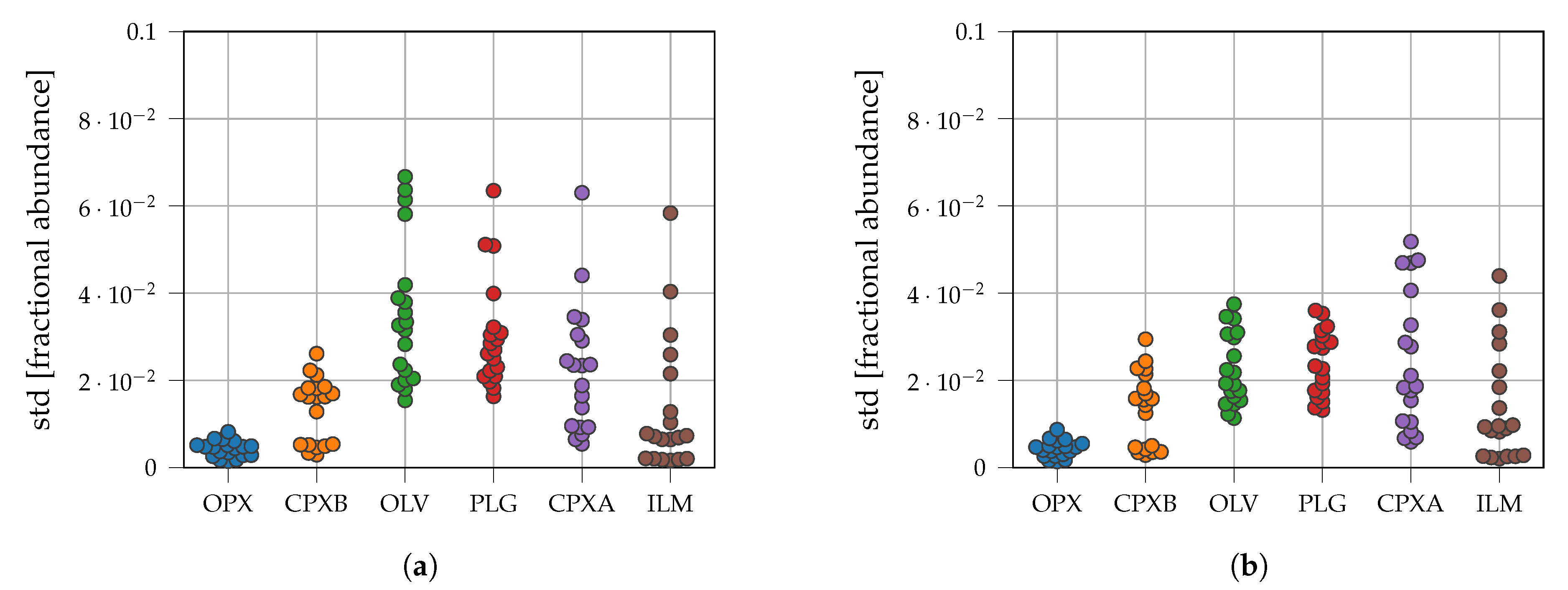
The abundance of npFe0 and mpFe0 is usually well defined, as changes to the abundance of npFe0 and mpFe0 can have a strong influence on the modeled spectrum. In Figure 7, Figure 8 and Figure 10 it can be seen that the predicted npFe0 and mpFe0 do not change significantly with the introduction of a prior. In Table 3 the correlation coefficients between true smFe abundance and the standard deviation of the minerals is listed. For all minerals it can be seen that the correlation coefficients are positive. Therefore, the higher the abundance of smFe is, the larger the uncertainties become. The uncertainty of ilmenite is, however, uncorrelated to the smFe abundance, even if no prior knowledge is used. Because ilmenite does not show a prominent absorption band such a feature cannot be obscured by the smFe particles. This is visible in Figure 13. While the overall uncertainties decrease with a prior on the elemental abundances, the trend that the uncertainties increase with increasing maturity is visible for both with and without a prior.
Generally, it can be seen that the ilmenite abundance is difficult to determine reliably without prior information, for both immature and mature spectra. For mature spectra, the uncertainties of all mineral abundances become very large, even for an almost perfect case, where influences which are not modeled, are removed. This illustrates that unmixing on the Moon is an ill-posed problem, and additional knowledge about the composition is necessary. The addition of a prior to indirectly include information about the plagioclase and ilmenite abundance is effective in reducing some of the uncertainties.
3.2. Fresh Laboratory Mixtures
This experiment is set up to unmix real laboratory mixtures (see also Rommel et al. [13]) from laboratory endmembers. Thus, we select the same endmembers as in Rommel et al. [13] but omit one of the two labradorites (plagioclases) as the two are very similar, and we want to select endmembers that are spectrally distinct. We also omit the diallagite endmember, to reduce the catalog to the same size as for the other experiments and this endmember is only present in one mixture, which is, consequently, also omitted here. The amphibole endmember pargasite (PRG) was selected in Rommel et al. [13] to test whether uncommon minerals can also be detected by the algorithm. We keep this endmember for our analysis even though it is not present on the Moon.
For the inversion of the Hapke model, the parameters are chosen in the same way as in Rommel et al. [13] for comparability. Therefore, the term for the shadow hiding opposition effect is not set to zero, but = 3.1 and = 0.11 are adopted from Rommel et al. [13]. The resulting SSA spectra are shown in Figure 14.
The elemental abundances of the endmembers were determined in Rommel et al. [13] based on electron microprobe analysis in the laboratory (see Table A5) and the modes and shape parameters are determined according to Section 2.2.3. The results were obtained by using no elemental priors on the one hand and using a prior for the TiO2 abundance on the other hand (see first two rows of Table 2).
The true values of the abundance of submicroscopic iron particles in this experiment is zero. In order to test whether fresh and mature spectra can be reliably distinguished from each other, we still employ the same prior for smFe as for the other experiments.
All endmembers and mixtures were measured in the same laboratory and the mixtures are directly mixed from the endmembers; therefore, the weights of the endmembers should sum up to a value close to one. We set a prior on the sum according to Equation (17) with a standard deviation of .
The detailed results of the unmixing without a prior on the elemental abundances and with a prior on the TiO2 abundance are listed in Table A7 and Table A8, respectively. Generally, the mean predicted results are very similar to those of Rommel et al. [13] considering that the endmembers labradorite A and diallagite were omitted. Even though we did not use a strong prior on the abundance of iron particles, the predicted abundances are almost exclusively below 0.02 wt.% or a fraction smaller than .
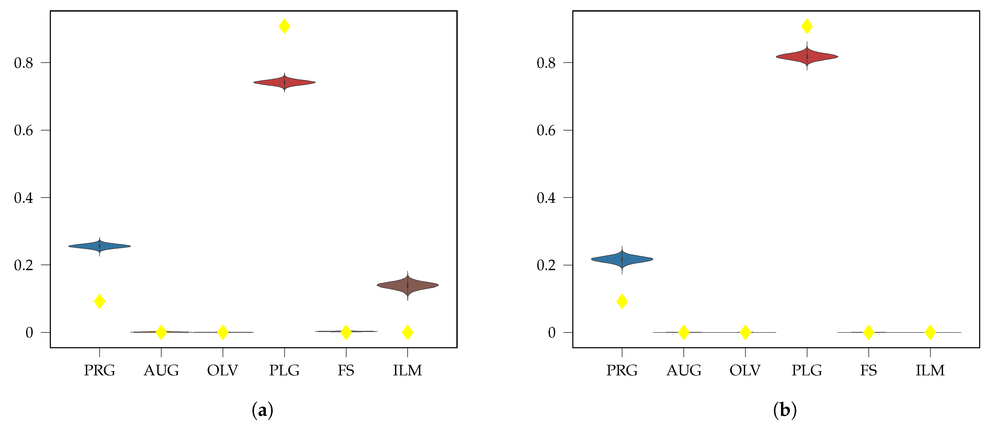
For the version without a prior on the TiO2 abundance, ilmenite is erroneously predicted in the mixtures of pargasite and plagioclase. For example, Figure 15 shows the violin plots of all similarly well-fitting solutions. It can be seen that ilmenite is predicted to be present, and a solution without ilmenite is not part of the uncertainty. Therefore, a solution with ilmenite fits better than one without ilmenite. If we, however, prefer solutions where the contribution of ilmenite is close to zero, we obtain a better result and the errors in pargasite and plagioclase abundance are reduced. In Figure 16 the confidence plots are plotted. Here it can be seen that the mean and mode predicted spectra fit quite well for both prior setups. By introducing the prior for the TiO2 abundance, the uncertainties of the fit increase ( = 0.006 compared to = 0.003 for no prior). Therefore, slightly less well fitting solutions are accepted if the ilmenite abundance confirms better with the prior knowledge.
In the mixtures containing plagioclase and ferrosilite, plagioclase is confused with pargasite if no prior knowledge is included. The two endmembers are spectrally very similar and are both bright (see Figure 14). In Figure 17, an example violin plot is shown, where the confusion of plagioclase and pargasite can be seen in Figure 17a. Small contributions of ilmenite can already dampen the absorption band of the pargasite endmember, such that the similarity to plagioclase increases. The mean predicted abundance of ilmenite is quite low with 0.48 wt.% for the version without a prior, but still leads to a significantly different solution. The confidence plots in Figure 18 look nearly identical, except that for the TiO2 prior to the uncertainty of the 0.9 m absorption band slightly increases. This suggests that both solutions, with and without ilmenite, represent regions of high posterior density. It is, however, very difficult for the sampler to traverse from one region to the other, as the two are far apart and due to the prior on the sum it is unlikely for a limited number of samples that both regions are sampled. However, with a relatively uninformative prior as in Figure 6 this ambiguity can be removed, such that the solutions with no ilmenite are preferred. This trend illustrated by the two examples above, can also be seen in Figure 19. The differences between mean predicted solution and true abundance for the endmembers augite, olivine, and ferrosilite are not improved by including prior knowledge about the TiO2 abundance. This is likely because of inaccuracies of the data and the simple mixing model and also a problem in Rommel et al. [13]. The inherent simplifications of the Hapke model makes it such that the fractional abundances are not necessarily equal to their actual weight fraction (e.g., [56]). Similar to a regularization term in classical optimizations, we can use the prior to favor certain solutions, without imposing hard constraints. Generally, without prior knowledge the abundance of plagioclase is usually underestimated, while the abundance of ilmenite and pargasite is overestimated. The uncertainties are mostly small, both with and without TiO2 prior (see Figure 20).
3.3. LSCC Samples
In the final experiment, we unmix spectra from the LSCC catalog with laboratory mineral endmembers and the npFe0 and mpFe0 particles. The LSCC catalog contains mature samples that were returned from the lunar surface by the Apollo missions and is, therefore, a good representation of lunar mineralogy. We use the <45 m size fraction spectra for the unmixing, and because there is no data on the mineral abundances of this size fraction we use the mineral abundances from the 20–45 m size fraction, which correspond to a large portion of the weight, as a reference for evaluating the results. The endmembers are the same samples from the RELAB library listed in Section 3.1. These endmembers do not correspond to the actual constituent minerals and there are additional minerals that are not covered by the endmember catalog, for example, spinel. Additionally, the endmember catalog does not contain agglutinates in comparison to the LSCC samples with large fractions of agglutinates. The ground truth abundances are obtained from the tables of Taylor et al. [18,19]. The abundances of the minerals were grouped into clinopyroxene, orthopyroxene, olivine, plagioclase, and ilmenite. The abundances were then normalized to the mineral fraction because we are not considering glasses. We have seen that, without a prior on the elemental abundances, the uncertainties become very large for mature spectra. Therefore, we will use the same prior once on TiO2 and Al2O3 abundances, which in the previous experiments reduced the uncertainties effectively for plagioclase and ilmenite, but also for many of the other minerals. Additionally, we will employ a prior on all elements with a relevant abundance on the Moon, which might contribute to distinguishing between minerals (see also Table 2). The elemental abundances of the LSCC samples are listed in Table A9. The spectra were measured under laboratory conditions, but the mixtures are much more complex compared to the laboratory mixtures from Section 3.2. We are, therefore, not enforcing the sum-to-one constraint as strongly, as we set . Because plagioclase and ilmenite have both almost featureless flat spectra, the uncertainties between these two increase significantly the more relaxed the prior on the sum is. Therefore, the prior knowledge about TiO2 and Al2O3 abundance becomes even more essential.
Detailed results for the unmixing of all LSCC spectra are listed in Table A10 and Table A11 for the two experiments with different priors. Generally, the uncertainties are similar between both versions, but for some samples the priors on the other elements help in reducing the uncertainties. This can be seen in Figure 21. Therefore, we will focus on the Ti/Al prior version.
In some cases, the plagioclase abundance is underestimated; such an example can be seen in Figure 22. For the violin plots, the two clinopyroxenes are grouped together. The spectrum fits quite well and the true plagioclase abundance is not part of the uncertainty. Therefore, a prior cannot mitigate the differences between mean predicted and theoretical abundance. Instead, olivine and orthopyroxene abundances are overestimated. A similar problem can be seen for 12001 and 15041. These samples are the ones with the highest fraction of agglutinic glasses (12001: 56.2 wt%, and 15041: 51.3 wt%, and 10084: 53.9 wt%) among the mare samples. For all other samples, the predicted abundances are close to the true values.
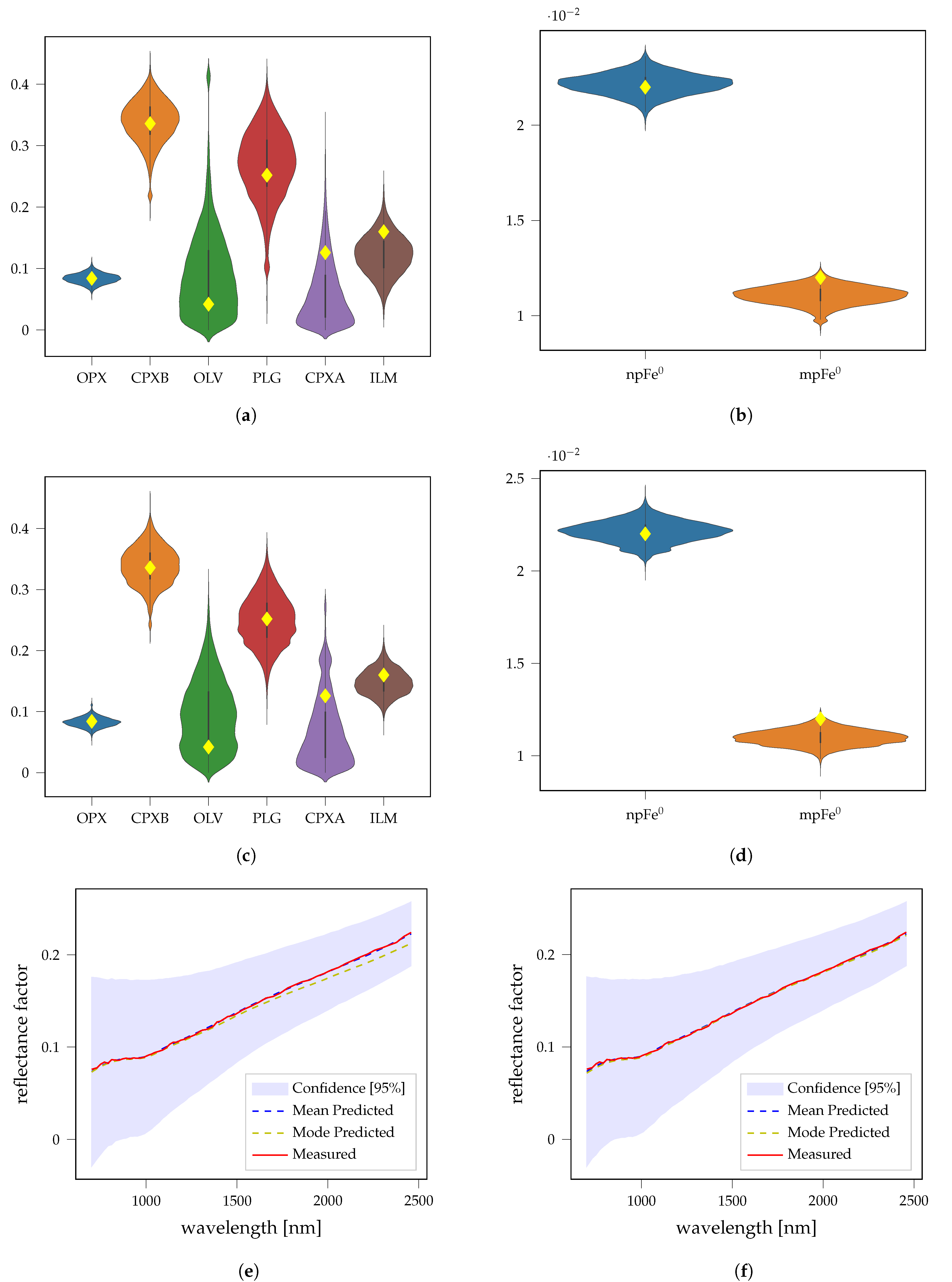
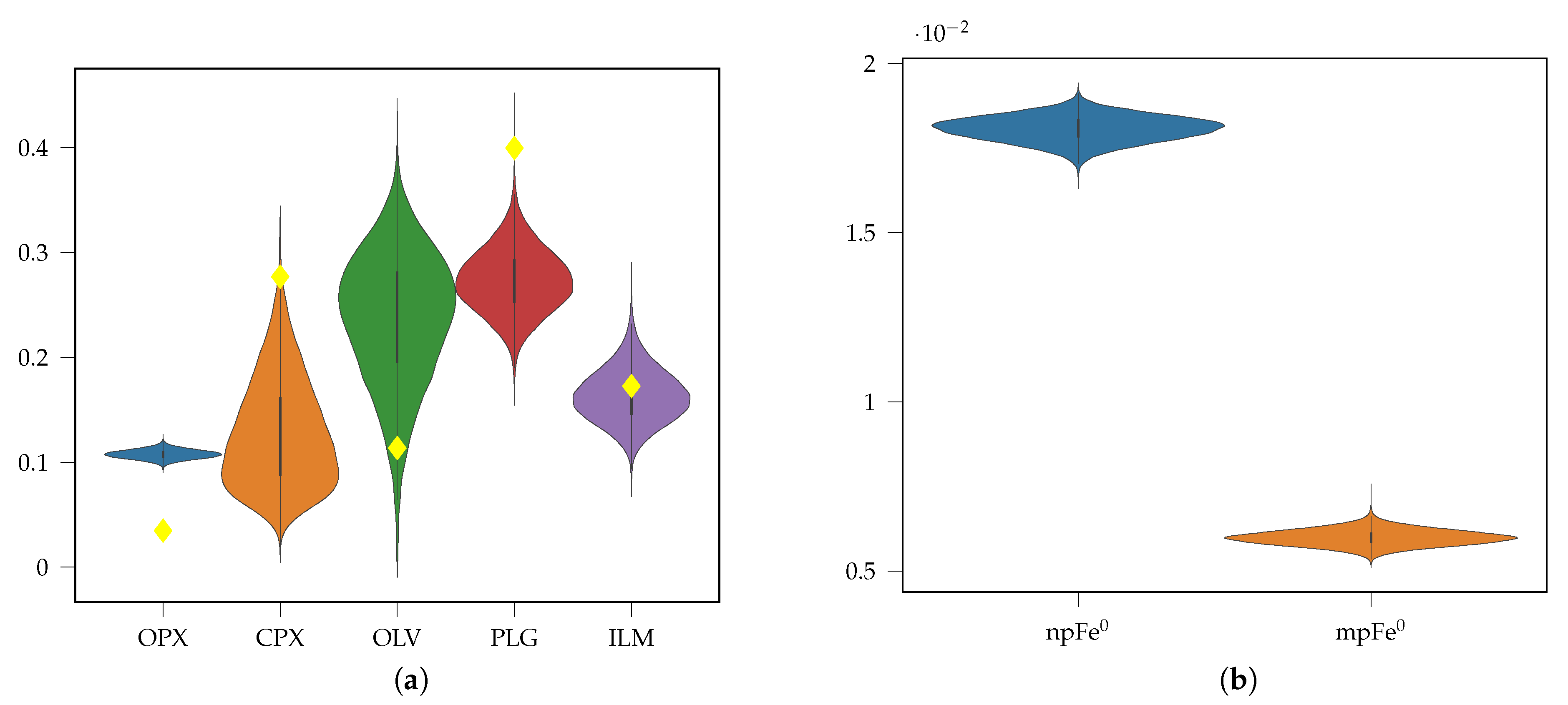
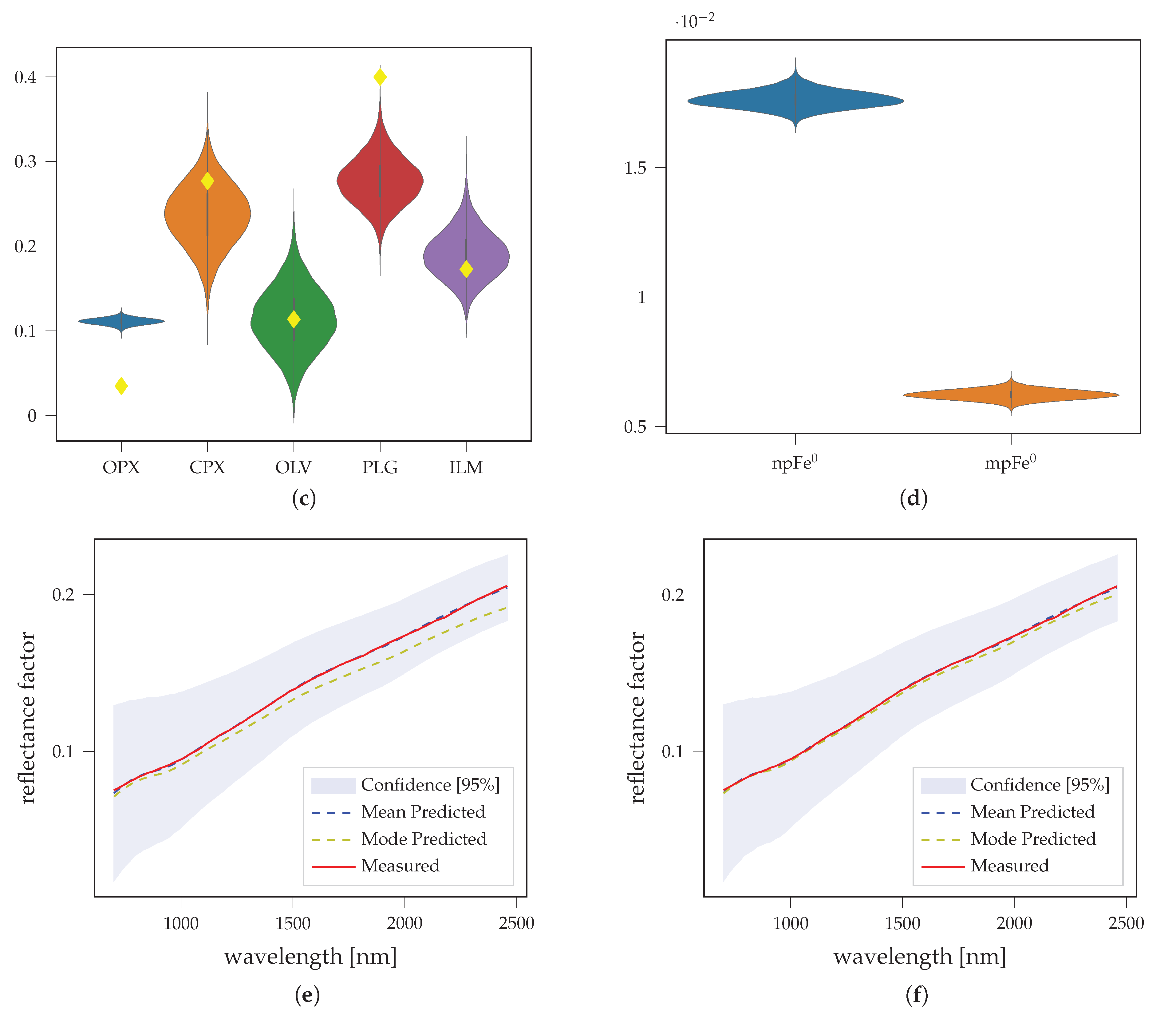
Figure 23 shows the typical results for a mature mare spectrum. Most of the abundances are relatively well defined with the prior on the TiO2 and Al2O3 abundance. Compared to sample 10084 in Figure 22, there are significantly fewer npFe0 and mpFe0 particles predicted to be present. As sample 14260 contains less FeO (9.65 wt.% compared to 14.8 wt.% in 10084) it is likely that the smFe abundance saturates more quickly, such that additional smFe cannot easily be created as quickly anymore. The ilmenite abundance is comparatively small, which might also be a contributing factor to the uncertainties being relatively small. Similarly, for the mature highland spectrum in Figure 24, the iron abundance in the highlands is generally much smaller so that less smFe can be created. According to the Is/FeO parameter, this is also a very mature spectrum and the absorption bands are weakly pronounced. However, the smFe abundance is small compared to the mare samples. In Figure 25, the results for sample 79221, with both the Ti/Al prior and also with the prior on all major elemental abundances, is shown. This sample is rich in ilmenite and also relatively mature, therefore the uncertainties are quite high. In such cases, the results can be improved when additional elemental abundance information is available. For most other LSCC samples the Ti/Al prior is, however, sufficient to constrain the procedure. The npFe0 and mpFe0 abundance is not much effected by the change in prior knowledge.
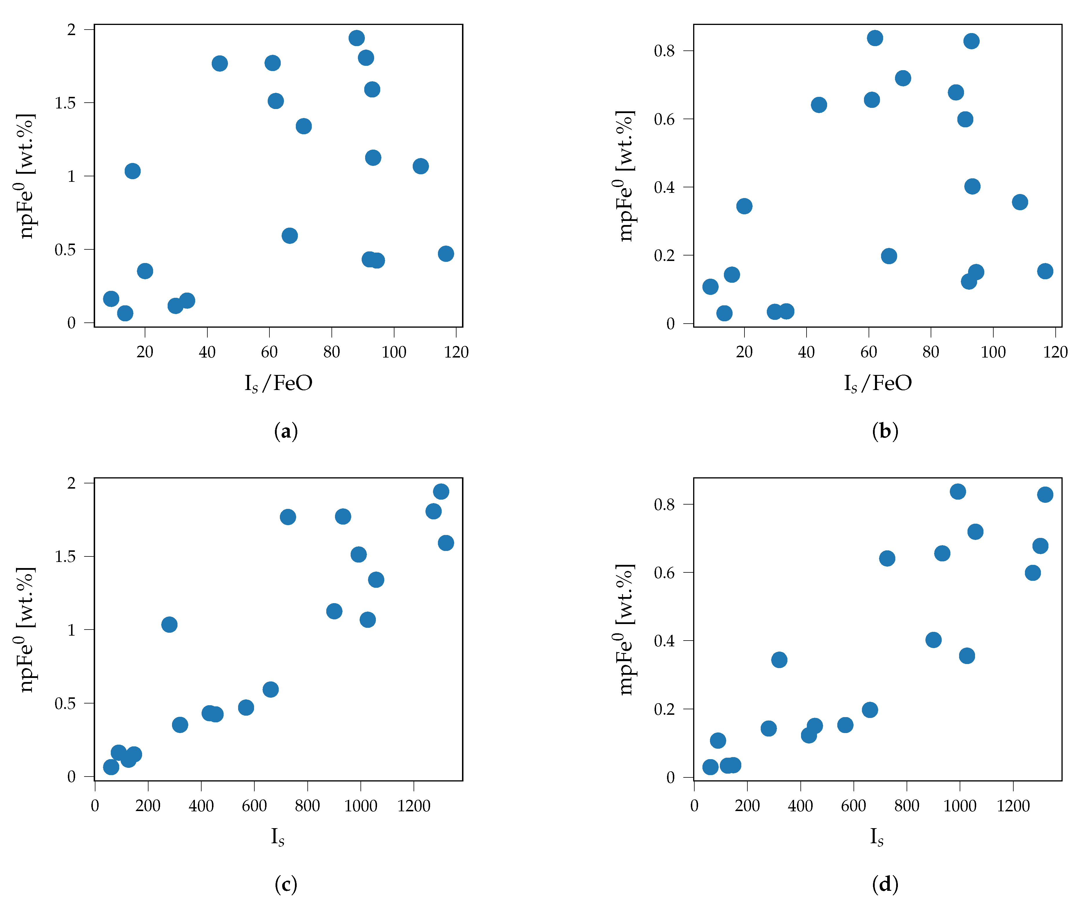
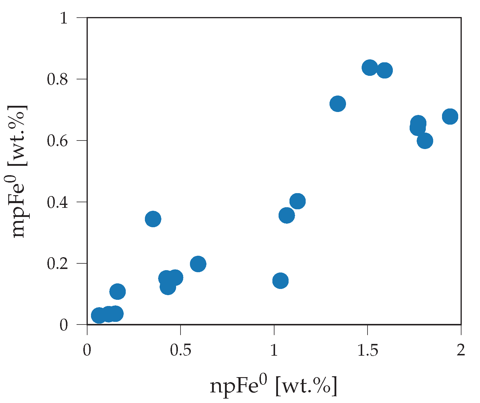
In Figure 26 the correlations between Is/FeO or Is and mean predicted npFe0 or mpFe0 abundance are displayed. The abundances are only weakly correlated with the Is/FeO maturity index. In contrast the correlation between the ferromagnetic resonance Is and the abundance is very strong. Even for the small dataset this correlation is significant. Because the Is is a measure on the amount of iron particles in the size fraction between 4 nm and 33 nm [57], this suggests that the abundance of npFe0 can be obtained relatively reliably even with a limited endmember catalog. This difference between Is/FeO and Is also supports the findings of Trang and Lucey [54] that the saturation limit of npFe0 particles is dependent on the FeO abundance. The saturation limit increases with increasing FeO abundance. Figure 27 shows the relationship between npFe0 and mpFe0 abundance in the LSCC samples. Usually, the factor between the abundance of npFe0 and mpFe0 abundance is approximately constant, where the amount of npFe0 is typically twice as high as the amount of mpFe.
4. Discussion
Generally, the three experiments show that a probabilistic perspective provides important insights into the unmixing process overall. When trying to unmix lunar spectra many factors have to be considered to obtain reliable results. A non-probabilistic approach needs to make many assumptions about the composition and the maturity of the surface to obtain plausible results. Even if these assumptions are accurate only a single best fit solution is obtained. All experiments shown in this work illustrate that there is no unique solution and that a variety of combinations can produce similar results and, thus, a number of different interpretations are possible.
The synthetic mixtures in Section 3.1 were used to estimate the influence of the darkening agents on the overall uncertainties of the mineral abundances. The results showed that with increasing smFe abundance the uncertainties increased. Ilmenite or TiO2 also contributed to uncertainties in the data, but there appears to be no direct relationship between true ilmenite abundance and uncertainties. However, introducing prior knowledge about the TiO2 and Al2O3 abundance can significantly reduce the uncertainties of all mineral abundances as well as the errors between mean predicted and true mineral abundances and is, therefore, suitable for the application of the approach to real lunar spectra. For very mature spectra the uncertainties become very large. This illustrates the need for a probabilistic approach to the problem of unmixing spectra for mineral and smFe particle abundances. The abundance of the smFe particles could, however, still be reliably detected for any maturity level. The uncertainties of the minerals all increased with increasing smFe concentration, except for ilmenite. This might be explained by the fact that ilmenite with its featureless spectrum is already difficult to determine accurately if the absolute brightness of the sample is not well defined. Ilmenite, therefore, is not easily distinguished by any absorption bands, which become more difficult to quantify with increasing maturity.
Ambiguities between spectrally similar endmembers such as plagioclase, pargasite, and ilmenite in Section 3.2 can lead to larger errors (up to 57 wt.%) in the best fit solution of the Hapke model and the measured spectra. When these ambiguities are mitigated with using prior information, the errors are usually well below 15 wt.%. All models have to include some simplifications such that they cannot perfectly represent reality. These problems inherent to the mixing model itself usually cannot be predicted by the MCMC sampler. Ambiguities and uncertainties due to the choice of model parameters on the other hand can be quantified and may indicate problems with the choice of endmembers and/or assumptions made about the data. In some cases where plagioclase and pargasite were confused, two local minima far apart from each other in parameter space were not found by the sampler, even though the mean of the confidence plots is very similar. Generally, the fresh laboratory spectra could easily be distinguished as such. The abundance of smFe is predicted to be effectively absent.
The final experiment of unmixing the LSCC spectra with RELAB mineral endmembers demonstrated that this approach can be applied to the lunar surface. When the abundance of agglutinitic glasses is high, olivine and plagioclase abundances tend to be poorly defined. The reconstruction is very accurate, but the uncertainties of the mineral abundances are high for mature spectra. This shows that classical optimization techniques are prone to fail on the task of unmixing the spectra with accurate abundances. The abundances of the smFe particles are, however, well defined. The results align with the findings of Trang and Lucey [54] that the npFe and mpFe abundance for mature spectra depends on the FeO abundance. Furthermore, the predicted abundance of npFe and mpFe particles correlates well with the Is parameter of the LSCC samples. For npFe, this can be interpreted to be a sign that the algorithm predicts plausible results. The npFe and mpFe abundances are also strongly correlated, such that the correlation of mpFe might be attributed to this nearly constant factor. According to Lucey and Riner [16] mpFe sized particles are not present in the samples investigated, but the larger particle size is necessary to model the effects of space weathering. Wohlfarth et al. [24] further suggested that clusters or layers of npFe particles that effectively act as a larger mpFe particle are responsible for the darkening. This effect can also be simulated with light scattering theory as in Arnaut et al. [58]. This would suggest that npFe and mpFe (or clusters of npFe) are both created by the same processes. The cluster/layer theory is consistent with the results of the LSCC unmixing.
All endmembers and investigated mixtures have the same average grain size, which usually is not the case for remotely measured datasets. For the Martian surface, Lapotre et al. [22] and Lapotre et al. [59] investigated the influence of the grain size on the uncertainties and showed that the solution to this inverse problem is highly non-unique. Integrating the grain size into the existing framework would add another layer of complexity to the model, making it even more challenging to obtain meaningful results. Therefore, prior knowledge about the grain size would likely be necessary to constrain the procedure. If the grain size varied significantly between endmembers, systematical errors with respect to their relative fraction would be introduced. Some simplifications to the model, however, have to be made for this highly complex inverse problem to be solvable. The effects of the grain size in combination with space weathering components and the other agents that darken the overall spectrum, discussed in this work, can be investigated in possible future research.
The laboratory samples examined in this work all have a relatively high SNR in comparison to, for example, the Moon Mineralogy Mapper data. When the SNR decreases, the standard deviation of the likelihood function is likely to increase, such that more solutions might be considered acceptable. This, in turn, most likely also increases the uncertainties of the fractional abundances. Nonetheless, we can indirectly measure the influence of the SNR based on the average differences between model prediction and observed spectra. In our work, which follows a Bayesian approach, the variance of the differences is a part of the model and is thus also estimated (cf. Equation (13)). However, averaging over neighboring pixels, where the composition is similar, improves the SNR. Due to the high computational effort to sample from these complex distributions, the number of pixels that can be investigated is limited. Therefore, clustering the data and applying the unmixing to the centroids also mitigates the effects of a low SNR and makes computing the abundances over large areas feasible (e.g., [60,61]).
5. Conclusions
Unmixing can be used to obtain quantitative information about the composition of remote surfaces. Building on the Hapke model (e.g., [9]) and the space weathering model of Wohlfarth et al. [24], we have developed a combined unmixing model. The parameters of the model and their corresponding uncertainties were obtained by Bayesian inference with an MCMC sampler. The results showed that, especially on the Moon, there is no unique solution that would perfectly describe the measured spectra. The absorption bands at around 1-m and 2-m are the main features for estimating the abundances. These features are obscured by submicroscopic iron particles, making it harder to quantify the corresponding mineral abundances. Some mineral combinations even become gradually interchangeable, only slightly changing the modeled spectrum. Therefore, additional knowledge is necessary to constrain the procedure. We find that information about the elemental abundances, which can be obtained from different independent data sources, is well suited to helping to distinguish between different minerals and we prefer solutions that correspond better with this prior knowledge. Inherent simplifications of the mixing model can lead to systematic errors. In such cases, the uncertainties might still be small, therefore, it is difficult to predict such problems with the model itself if no ground truth is available. Overall, the uncertainties can be accurately estimated from the MCMC sampler. For very mature spectra, these uncertainties become large, suggesting that a classical optimization approach is destined to fail at consistently predicting accurate results. The abundance of submicroscopic iron particles, responsible for the optical effects of maturity, could reliably be determined with the proposed approach. The results of the unmixing on LSCC spectra showed that the probabilistic unmixing approach is applicable to realistic lunar spectra. The knowledge about the uncertainties inherent to the problem are, however, essential for the interpretation of the results obtained for lunar spectra.
Author Contributions
Conceptualization, M.H., T.W. and C.W.; methodology, M.H., T.W. and K.W.; software, M.H.; validation, M.H.; formal analysis, M.H.; investigation, M.H.; data curation, M.H.; writing—original draft preparation, M.H.; writing—review and editing, T.W., C.W. and K.W.; visualization, M.H.; supervision, C.W. All authors have read and agreed to the published version of the manuscript.
Funding
Thorsten Wilhelm and Christian Wöhler acknowledge funding from the Deutsche Forschungsgemeinschaft (DFG, German Research Foundation) project number 269661170.
Data Availability Statement
RELAB database (https://pds-geosciences.wustl.edu/spectrallibrary/default.htm, accessed on 1 November 2021). LSCC catalog of lunar returned samples (https://pgi.utk.edu/lunar-soil-characterization-consortium-lscc-data/, accessed on 12 October 2021). Laboratory mineral and mixture spectra from Rommel et al. [13].
Acknowledgments
We want to thank the RELAB and LSCC teams for making the data to the catalog of spectra available publicly. We also want to thank Daniela Rommel for all the hard work, measuring the spectra and preparing the mixtures in Section 3.2. And finally the authors wish to thank the Department of Geochemistry of the University of Göttingen for providing the mineral samples examined in Section 3.2.
Conflicts of Interest
The authors declare no conflict of interest.
Appendix A
Appendix A.1. Synthetic Mixtures

Table A1.
Elemental abundances of endmember catalog for experiments in Section 3.1 and Section 3.3. The sample spectra and elemental abundances are taken from the RELAB library (https://pds-geosciences.wustl.edu/spectrallibrary/default.htm, accessed on 1 November 2020).
Table A1.
Elemental abundances of endmember catalog for experiments in Section 3.1 and Section 3.3. The sample spectra and elemental abundances are taken from the RELAB library (https://pds-geosciences.wustl.edu/spectrallibrary/default.htm, accessed on 1 November 2020).
| SiO2 | TiO2 | Al2O3 | Cr2O3 | MgO | CaO | MnO | FeO | Na2O | K2O | P2O5 | Fe2O3 | |
|---|---|---|---|---|---|---|---|---|---|---|---|---|
| AG-TJM-009 | 54.09 | 0.16 | 1.23 | 0.75 | 26.79 | 1.52 | 0.49 | 15.22 | 0.05 | 0.05 | 0.0 | 0.00 |
| AG-TJM-010 | 50.73 | 0.74 | 8.73 | 0.00 | 16.65 | 15.82 | 0.13 | 5.37 | 1.27 | 0.00 | 0.0 | 1.08 |
| PO-EAC-056 | 40.42 | 0.00 | 0.03 | 0.13 | 48.25 | 0.19 | 0.15 | 11.11 | 0.00 | 0.00 | 0.0 | 0.00 |
| PL-EAC-029 | 54.85 | 0.06 | 27.71 | 0.02 | 0.00 | 10.97 | 0.01 | 0.00 | 5.15 | 0.40 | 0.0 | 0.46 |
| PP-ALS-105 | 48.41 | 1.05 | 5.29 | 0.03 | 12.37 | 22.15 | 0.26 | 6.15 | 0.36 | 0.00 | 0.0 | 3.79 |
| SC-EAC-034 | 0.20 | 47.61 | 0.01 | 0.02 | 0.01 | 0.00 | 0.02 | 45.43 | 0.00 | 0.00 | 0.0 | 0.00 |
Table A2.
Origin of endmember samples in Section 3.1 and Section 3.3. All samples except for the AG-TJM-009 Hypersthene endmember, which is of meteoritic origin, originate from Earth.
Table A2.
Origin of endmember samples in Section 3.1 and Section 3.3. All samples except for the AG-TJM-009 Hypersthene endmember, which is of meteoritic origin, originate from Earth.
| Sample ID | Mineral | Origin | Abbreviation |
|---|---|---|---|
| AG-TJM-009 | Hypersthene | Johnstown Meteorite | OPX |
| AG-TJM-010 | Augite | Kakanui, New Zealand | CPXB |
| PO-EAC-056 | Olivine | Green sand beach near S Point, HI | OLV |
| PL-EAC-029 | Plagioclase | Ylijarvi, Ylamaaa, Kimi, Finland | PLG |
| PP-ALS-105 | Diopside | Trail Creek, Grand Co., CO | CPXA |
| SC-EAC-034 | Ilmenite | Telemark, Norway | ILM |
Table A3.
Detailed results for the unmixing of the synthetically generated by using the forward mixing model. Only a uniform prior on the elemental and mineral abundances was set.
Table A3.
Detailed results for the unmixing of the synthetically generated by using the forward mixing model. Only a uniform prior on the elemental and mineral abundances was set.
| mix0 | mix1 | mix2 | ||||||||||
|---|---|---|---|---|---|---|---|---|---|---|---|---|
| Mode | Mean | Std | Theo | Mode | Mean | Std | Theo | Mode | Mean | Std | Theo | |
| OPX | 9.97 | 9.96 | 0.04 | 10.00 | 9.80 | 9.82 | 0.14 | 10.00 | 10.76 | 10.66 | 0.27 | 10.00 |
| CPXB | 39.95 | 40.00 | 0.17 | 40.00 | 40.19 | 40.33 | 0.89 | 40.00 | 37.31 | 37.75 | 1.58 | 40.00 |
| OLV | 4.58 | 4.44 | 0.36 | 5.00 | 8.29 | 8.35 | 1.84 | 5.00 | 18.28 | 19.20 | 3.19 | 5.00 |
| PLG | 29.85 | 29.93 | 0.41 | 30.00 | 29.11 | 28.45 | 1.71 | 30.00 | 13.89 | 16.75 | 3.05 | 30.00 |
| CPXA | 15.02 | 15.38 | 0.50 | 15.00 | 12.60 | 12.43 | 2.13 | 15.00 | 18.96 | 13.99 | 3.56 | 15.00 |
| ILM | 0.17 | 0.83 | 0.63 | 0.00 | 0.52 | 1.50 | 1.21 | 0.00 | 2.03 | 3.60 | 2.21 | 0.00 |
| npFe | 0.00 | 0.00 | 0.00 | 0.00 | 0.00 | 0.00 | 0.00 | 0.00 | 0.00 | 0.01 | 0.01 | 0.00 |
| mpFe | 0.00 | 0.00 | 0.00 | 0.00 | 0.40 | 0.40 | 0.00 | 0.40 | 0.78 | 0.79 | 0.01 | 0.80 |
| SUM | 99.55 | 100.54 | 100.00 | 100.51 | 100.87 | 100.00 | 101.23 | 101.96 | 100.00 | |||
| mix3 | mix4 | mix5 | ||||||||||
| Mode | Mean | Std | Theo | Mode | Mean | Std | Theo | Mode | Mean | Std | Theo | |
| OPX | 10.07 | 9.91 | 0.34 | 10.00 | 10.34 | 10.46 | 0.19 | 10.00 | 9.87 | 9.87 | 0.24 | 10.00 |
| CPXB | 35.50 | 39.32 | 1.69 | 40.00 | 38.56 | 39.69 | 1.30 | 40.00 | 38.72 | 38.86 | 1.60 | 40.00 |
| OLV | 40.64 | 32.95 | 5.25 | 5.00 | 6.37 | 2.48 | 2.05 | 5.00 | 7.98 | 8.40 | 4.56 | 5.00 |
| PLG | 1.60 | 12.86 | 4.53 | 30.00 | 25.96 | 28.15 | 1.97 | 30.00 | 27.49 | 27.86 | 2.83 | 30.00 |
| CPXA | 7.46 | 2.73 | 2.17 | 15.00 | 18.36 | 18.76 | 2.92 | 15.00 | 13.56 | 13.21 | 5.03 | 15.00 |
| ILM | 9.80 | 4.19 | 2.49 | 0.00 | 0.24 | 1.62 | 1.40 | 0.00 | 4.30 | 4.61 | 2.42 | 0.00 |
| npFe | 0.07 | 0.05 | 0.01 | 0.00 | 0.57 | 0.57 | 0.01 | 0.60 | 0.60 | 0.61 | 0.02 | 0.60 |
| mpFe | 1.18 | 1.16 | 0.02 | 1.20 | 0.01 | 0.01 | 0.00 | 0.00 | 0.40 | 0.40 | 0.01 | 0.40 |
| SUM | 105.08 | 101.95 | 100.00 | 99.82 | 101.15 | 100.00 | 101.93 | 102.81 | 100.00 | |||
| mix6 | mix7 | mix8 | ||||||||||
| Mode | Mean | Std | Theo | Mode | Mean | Std | Theo | Mode | Mean | Std | Theo | |
| OPX | 8.69 | 8.63 | 0.33 | 10.00 | 10.52 | 10.68 | 0.58 | 10.00 | 11.43 | 11.64 | 0.39 | 10.00 |
| CPXB | 46.15 | 45.51 | 1.59 | 40.00 | 33.21 | 39.95 | 2.91 | 40.00 | 33.81 | 31.75 | 2.44 | 40.00 |
| OLV | 18.74 | 14.98 | 5.36 | 5.00 | 10.37 | 11.96 | 7.17 | 5.00 | 11.08 | 2.41 | 2.63 | 5.00 |
| PLG | 26.56 | 26.74 | 4.51 | 30.00 | 21.10 | 29.30 | 5.31 | 30.00 | 19.85 | 18.35 | 2.76 | 30.00 |
| CPXA | 0.51 | 2.26 | 2.07 | 15.00 | 23.73 | 7.81 | 5.97 | 15.00 | 22.63 | 35.25 | 5.78 | 15.00 |
| ILM | 1.76 | 4.32 | 2.50 | 0.00 | 1.63 | 1.90 | 1.55 | 0.00 | 0.69 | 1.64 | 1.38 | 0.00 |
| npFe | 0.68 | 0.69 | 0.02 | 0.60 | 0.55 | 0.57 | 0.03 | 0.60 | 1.34 | 1.32 | 0.02 | 1.40 |
| mpFe | 0.75 | 0.76 | 0.02 | 0.80 | 1.28 | 1.29 | 0.03 | 1.20 | 0.01 | 0.01 | 0.00 | 0.00 |
| SUM | 102.41 | 102.45 | 100.00 | 100.56 | 101.60 | 100.00 | 99.48 | 101.04 | 100.00 | |||
| mix9 | mix10 | mix11 | ||||||||||
| Mode | Mean | Std | Theo | Mode | Mean | Std | Theo | Mode | Mean | Std | Theo | |
| OPX | 10.68 | 10.46 | 0.49 | 10.00 | 9.71 | 9.44 | 0.37 | 10.00 | 9.77 | 8.86 | 0.54 | 10.00 |
| CPXB | 39.80 | 36.92 | 2.93 | 40.00 | 43.59 | 44.30 | 1.60 | 40.00 | 39.64 | 46.41 | 2.76 | 40.00 |
| OLV | 7.62 | 9.75 | 6.68 | 5.00 | 5.39 | 5.74 | 3.67 | 5.00 | 8.74 | 9.25 | 5.80 | 5.00 |
| PLG | 22.46 | 22.45 | 3.81 | 30.00 | 34.59 | 36.19 | 2.89 | 30.00 | 20.78 | 27.35 | 4.11 | 30.00 |
| CPXA | 4.62 | 19.44 | 8.02 | 15.00 | 7.01 | 3.59 | 2.98 | 15.00 | 20.16 | 7.79 | 5.47 | 15.00 |
| ILM | 0.49 | 1.74 | 1.46 | 0.00 | 0.13 | 2.07 | 1.59 | 0.00 | 1.78 | 1.54 | 1.31 | 0.00 |
| npFe | 1.40 | 1.40 | 0.04 | 1.40 | 1.44 | 1.46 | 0.02 | 1.40 | 1.38 | 1.44 | 0.03 | 1.40 |
| mpFe | 0.37 | 0.37 | 0.02 | 0.40 | 0.81 | 0.79 | 0.02 | 0.80 | 1.18 | 1.22 | 0.03 | 1.20 |
| SUM | 85.67 | 100.77 | 100.00 | 100.41 | 101.33 | 100.00 | 100.88 | 101.19 | 100.00 | |||
| mix12 | mix13 | mix14 | ||||||||||
| Mode | Mean | Std | Theo | Mode | Mean | Std | Theo | Mode | Mean | Std | Theo | |
| OPX | 10.39 | 10.09 | 0.50 | 10.00 | 11.54 | 11.44 | 0.48 | 10.00 | 6.48 | 6.71 | 0.60 | 10.00 |
| CPXB | 38.62 | 38.96 | 2.82 | 40.00 | 37.73 | 36.57 | 2.24 | 40.00 | 37.72 | 39.38 | 1.64 | 40.00 |
| OLV | 11.31 | 9.79 | 5.69 | 5.00 | 33.08 | 35.29 | 6.59 | 5.00 | 1.92 | 2.24 | 1.72 | 5.00 |
| PLG | 19.88 | 19.74 | 3.17 | 30.00 | 6.57 | 7.23 | 3.54 | 30.00 | 45.94 | 47.81 | 2.04 | 30.00 |
| CPXA | 23.44 | 20.65 | 7.95 | 15.00 | 12.51 | 7.60 | 5.67 | 15.00 | 6.13 | 2.57 | 1.89 | 15.00 |
| ILM | 1.69 | 1.81 | 1.49 | 0.00 | 1.56 | 1.93 | 1.56 | 0.00 | 2.10 | 1.77 | 1.43 | 0.00 |
| npFe | 2.15 | 2.15 | 0.04 | 2.20 | 2.22 | 2.23 | 0.03 | 2.20 | 2.25 | 2.29 | 0.04 | 2.20 |
| mpFe | 0.00 | 0.01 | 0.01 | 0.00 | 0.32 | 0.32 | 0.02 | 0.40 | 0.73 | 0.74 | 0.02 | 0.80 |
| SUM | 105.32 | 101.04 | 100.00 | 102.98 | 100.06 | 100.00 | 100.29 | 100.48 | 100.00 | |||
| mix15 | mix16 | mix17 | ||||||||||
| Mode | Mean | Std | Theo | Mode | Mean | Std | Theo | Mode | Mean | Std | Theo | |
| OPX | 10.29 | 11.09 | 0.74 | 10.00 | 9.17 | 9.16 | 0.07 | 9.20 | 9.07 | 9.07 | 0.18 | 9.20 |
| CPXB | 38.16 | 35.75 | 3.99 | 40.00 | 36.89 | 36.79 | 0.36 | 36.80 | 38.87 | 38.89 | 1.13 | 36.80 |
| OLV | 24.38 | 11.31 | 8.60 | 5.00 | 4.92 | 5.39 | 0.99 | 4.60 | 0.71 | 5.90 | 2.80 | 4.60 |
| PLG | 18.23 | 18.96 | 4.36 | 30.00 | 26.73 | 26.32 | 1.18 | 27.60 | 27.08 | 28.03 | 2.41 | 27.60 |
| CPXA | 0.59 | 21.99 | 10.56 | 15.00 | 13.71 | 13.66 | 1.51 | 13.80 | 17.80 | 9.52 | 3.24 | 13.80 |
| ILM | 1.96 | 1.53 | 1.31 | 0.00 | 9.98 | 9.87 | 1.98 | 8.00 | 15.51 | 9.71 | 2.56 | 8.00 |
| npFe | 2.17 | 2.17 | 0.06 | 2.20 | 0.00 | 0.00 | 0.00 | 0.00 | 0.01 | 0.01 | 0.01 | 0.00 |
| mpFe | 1.18 | 1.18 | 0.03 | 1.20 | 0.00 | 0.00 | 0.00 | 0.00 | 0.41 | 0.41 | 0.01 | 0.40 |
| SUM | 93.61 | 100.63 | 100.00 | 101.40 | 101.20 | 100.00 | 109.03 | 101.12 | 100.00 | |||
| mix18 | mix19 | mix20 | ||||||||||
| Mode | Mean | Std | Theo | Mode | Mean | Std | Theo | Mode | Mean | Std | Theo | |
| OPX | 9.04 | 9.10 | 0.30 | 9.20 | 10.37 | 10.39 | 0.33 | 9.20 | 8.69 | 8.68 | 0.20 | 9.20 |
| CPXB | 37.76 | 40.48 | 1.75 | 36.80 | 36.89 | 37.34 | 1.64 | 36.80 | 35.95 | 35.97 | 1.24 | 36.80 |
| OLV | 7.86 | 8.05 | 3.45 | 4.60 | 12.22 | 14.88 | 3.52 | 4.60 | 2.26 | 2.77 | 1.96 | 4.60 |
| PLG | 21.73 | 26.48 | 3.49 | 27.60 | 21.05 | 25.06 | 3.40 | 27.60 | 30.05 | 29.81 | 1.85 | 27.60 |
| CPXA | 16.18 | 9.28 | 3.77 | 13.80 | 9.78 | 4.85 | 2.97 | 13.80 | 15.59 | 14.84 | 3.51 | 13.80 |
| ILM | 5.82 | 4.08 | 2.38 | 8.00 | 7.95 | 6.38 | 2.67 | 8.00 | 8.06 | 7.69 | 2.65 | 8.00 |
| npFe | 0.00 | 0.01 | 0.01 | 0.00 | 0.00 | 0.01 | 0.01 | 0.00 | 0.60 | 0.60 | 0.01 | 0.60 |
| mpFe | 0.78 | 0.79 | 0.01 | 0.80 | 1.19 | 1.21 | 0.02 | 1.20 | 0.00 | 0.00 | 0.00 | 0.00 |
| SUM | 98.39 | 97.46 | 100.00 | 98.25 | 98.89 | 100.00 | 100.60 | 99.77 | 100.00 | |||
| mix21 | mix22 | mix23 | ||||||||||
| Mode | Mean | Std | Theo | Mode | Mean | Std | Theo | Mode | Mean | Std | Theo | |
| OPX | 9.75 | 9.52 | 0.30 | 9.20 | 10.59 | 10.38 | 0.41 | 9.20 | 9.86 | 8.92 | 0.51 | 9.20 |
| CPXB | 33.87 | 36.21 | 1.75 | 36.80 | 32.01 | 33.40 | 2.69 | 36.80 | 34.59 | 40.23 | 2.33 | 36.80 |
| OLV | 7.84 | 15.35 | 6.16 | 4.60 | 12.45 | 3.79 | 3.24 | 4.60 | 13.34 | 9.92 | 5.96 | 4.60 |
| PLG | 24.27 | 23.85 | 4.10 | 27.60 | 18.88 | 23.85 | 3.99 | 27.60 | 19.33 | 28.95 | 5.17 | 27.60 |
| CPXA | 13.79 | 7.67 | 5.11 | 13.80 | 18.51 | 21.58 | 6.11 | 13.80 | 13.03 | 4.22 | 3.59 | 13.80 |
| ILM | 7.95 | 5.71 | 2.72 | 8.00 | 5.91 | 5.00 | 2.67 | 8.00 | 12.18 | 7.87 | 3.06 | 8.00 |
| npFe | 0.58 | 0.61 | 0.02 | 0.60 | 0.58 | 0.57 | 0.02 | 0.60 | 0.64 | 0.65 | 0.02 | 0.60 |
| mpFe | 0.40 | 0.39 | 0.01 | 0.40 | 0.77 | 0.79 | 0.02 | 0.80 | 1.17 | 1.22 | 0.03 | 1.20 |
| SUM | 97.47 | 98.31 | 100.00 | 98.35 | 97.99 | 100.00 | 102.33 | 100.11 | 100.00 | |||
| mix24 | mix25 | mix26 | ||||||||||
| Mode | Mean | Std | Theo | Mode | Mean | Std | Theo | Mode | Mean | Std | Theo | |
| OPX | 8.76 | 8.84 | 0.34 | 9.20 | 7.97 | 7.87 | 0.45 | 9.20 | 8.51 | 8.31 | 0.57 | 9.20 |
| CPXB | 32.63 | 36.47 | 1.91 | 36.80 | 28.43 | 33.90 | 2.65 | 36.80 | 36.45 | 38.13 | 2.52 | 36.80 |
| OLV | 6.87 | 10.07 | 4.20 | 4.60 | 1.57 | 7.63 | 5.54 | 4.60 | 15.52 | 6.57 | 5.01 | 4.60 |
| PLG | 23.48 | 28.49 | 2.95 | 27.60 | 22.79 | 27.96 | 4.17 | 27.60 | 33.03 | 34.10 | 4.20 | 27.60 |
| CPXA | 19.23 | 8.47 | 5.43 | 13.80 | 31.63 | 15.13 | 7.00 | 13.80 | 0.47 | 6.23 | 5.01 | 13.80 |
| ILM | 9.69 | 6.86 | 2.81 | 8.00 | 2.91 | 4.79 | 2.65 | 8.00 | 3.55 | 5.38 | 2.75 | 8.00 |
| npFe | 1.41 | 1.41 | 0.02 | 1.40 | 1.42 | 1.41 | 0.03 | 1.40 | 1.42 | 1.43 | 0.03 | 1.40 |
| mpFe | 0.00 | 0.01 | 0.01 | 0.00 | 0.33 | 0.33 | 0.02 | 0.40 | 0.83 | 0.85 | 0.02 | 0.80 |
| SUM | 100.67 | 99.20 | 100.00 | 95.30 | 97.28 | 100.00 | 97.54 | 98.72 | 100.00 | |||
| mix27 | mix28 | mix29 | ||||||||||
| Mode | Mean | Std | Theo | Mode | Mean | Std | Theo | Mode | Mean | Std | Theo | |
| OPX | 10.58 | 10.40 | 0.73 | 9.20 | 9.85 | 9.22 | 0.51 | 9.20 | 8.96 | 7.92 | 0.64 | 9.20 |
| CPXB | 34.74 | 35.52 | 3.77 | 36.80 | 33.63 | 36.95 | 2.28 | 36.80 | 31.58 | 37.27 | 2.93 | 36.80 |
| OLV | 17.54 | 18.77 | 9.94 | 4.60 | 0.00 | 1.88 | 1.80 | 4.60 | 8.91 | 4.14 | 3.35 | 4.60 |
| PLG | 21.87 | 18.42 | 6.88 | 27.60 | 33.24 | 38.10 | 3.16 | 27.60 | 29.98 | 35.60 | 4.17 | 27.60 |
| CPXA | 9.78 | 10.64 | 7.87 | 13.80 | 6.55 | 7.37 | 4.35 | 13.80 | 13.88 | 8.37 | 5.73 | 13.80 |
| ILM | 3.61 | 4.75 | 2.76 | 8.00 | 6.40 | 3.35 | 2.26 | 8.00 | 4.02 | 5.15 | 2.80 | 8.00 |
| npFe | 1.35 | 1.34 | 0.04 | 1.40 | 2.17 | 2.19 | 0.03 | 2.20 | 2.12 | 2.21 | 0.04 | 2.20 |
| mpFe | 1.32 | 1.32 | 0.05 | 1.20 | 0.00 | 0.01 | 0.00 | 0.00 | 0.46 | 0.44 | 0.02 | 0.40 |
| SUM | 98.11 | 98.50 | 100.00 | 89.68 | 96.88 | 100.00 | 97.33 | 98.43 | 100.00 | |||
| mix30 | mix31 | mix32 | ||||||||||
| Mode | Mean | Std | Theo | Mode | Mean | Std | Theo | Mode | Mean | Std | Theo | |
| OPX | 7.81 | 7.53 | 0.62 | 9.20 | 9.09 | 8.67 | 0.77 | 9.20 | 8.39 | 8.42 | 0.11 | 8.40 |
| CPXB | 36.21 | 39.00 | 2.65 | 36.80 | 35.89 | 37.86 | 2.66 | 36.80 | 34.74 | 34.78 | 0.53 | 33.60 |
| OLV | 2.69 | 3.31 | 2.81 | 4.60 | 11.93 | 4.45 | 3.48 | 4.60 | 3.72 | 3.53 | 1.27 | 4.20 |
| PLG | 31.23 | 35.79 | 4.03 | 27.60 | 27.84 | 35.14 | 3.87 | 27.60 | 27.12 | 27.42 | 1.47 | 25.20 |
| CPXA | 15.27 | 7.14 | 5.08 | 13.80 | 8.12 | 5.79 | 4.24 | 13.80 | 10.13 | 10.02 | 1.77 | 12.60 |
| ILM | 5.71 | 4.99 | 2.62 | 8.00 | 2.77 | 5.02 | 2.72 | 8.00 | 15.86 | 15.64 | 2.28 | 16.00 |
| npFe | 2.23 | 2.25 | 0.04 | 2.20 | 2.28 | 2.27 | 0.05 | 2.20 | 0.00 | 0.00 | 0.00 | 0.00 |
| mpFe | 0.72 | 0.76 | 0.03 | 0.80 | 0.99 | 1.03 | 0.04 | 1.20 | 0.00 | 0.00 | 0.00 | 0.00 |
| SUM | 98.92 | 97.76 | 100.00 | 95.63 | 96.94 | 100.00 | 99.96 | 99.81 | 100.00 | |||
| mix33 | mix34 | mix35 | ||||||||||
| Mode | Mean | Std | Theo | Mode | Mean | Std | Theo | Mode | Mean | Std | Theo | |
| OPX | 8.88 | 8.81 | 0.20 | 8.40 | 8.65 | 8.31 | 0.41 | 8.40 | 9.12 | 8.35 | 0.54 | 8.40 |
| CPXB | 31.13 | 30.99 | 1.14 | 33.60 | 28.73 | 33.86 | 3.05 | 33.60 | 29.97 | 34.01 | 3.11 | 33.60 |
| OLV | 7.95 | 7.58 | 2.04 | 4.20 | 10.49 | 5.00 | 3.82 | 4.20 | 1.73 | 2.41 | 1.87 | 4.20 |
| PLG | 21.10 | 20.71 | 2.68 | 25.20 | 13.95 | 22.96 | 5.34 | 25.20 | 28.48 | 31.94 | 3.13 | 25.20 |
| CPXA | 15.73 | 15.24 | 2.63 | 12.60 | 23.20 | 15.10 | 6.09 | 12.60 | 16.19 | 8.71 | 5.22 | 12.60 |
| ILM | 17.80 | 17.59 | 2.72 | 16.00 | 11.53 | 12.02 | 2.84 | 16.00 | 12.27 | 11.80 | 2.47 | 16.00 |
| npFe | 0.00 | 0.00 | 0.00 | 0.00 | 0.01 | 0.02 | 0.01 | 0.00 | 0.01 | 0.02 | 0.01 | 0.00 |
| mpFe | 0.39 | 0.39 | 0.01 | 0.40 | 0.71 | 0.75 | 0.02 | 0.80 | 1.17 | 1.18 | 0.01 | 1.20 |
| SUM | 102.59 | 100.92 | 100.00 | 96.55 | 97.25 | 100.00 | 97.76 | 97.23 | 100.00 | |||
| mix36 | mix37 | mix38 | ||||||||||
| Mode | Mean | Std | Theo | Mode | Mean | Std | Theo | Mode | Mean | Std | Theo | |
| OPX | 8.92 | 8.83 | 0.23 | 8.40 | 8.29 | 8.18 | 0.33 | 8.40 | 8.87 | 8.70 | 0.35 | 8.40 |
| CPXB | 34.38 | 32.56 | 1.26 | 33.60 | 33.25 | 32.42 | 2.06 | 33.60 | 29.26 | 32.76 | 1.83 | 33.60 |
| OLV | 0.07 | 1.05 | 0.95 | 4.20 | 5.09 | 6.78 | 4.66 | 4.20 | 15.65 | 17.31 | 6.27 | 4.20 |
| PLG | 27.48 | 28.19 | 2.07 | 25.20 | 24.42 | 24.11 | 3.83 | 25.20 | 14.26 | 21.09 | 5.26 | 25.20 |
| CPXA | 10.38 | 14.40 | 2.78 | 12.60 | 0.91 | 12.18 | 5.67 | 12.60 | 13.64 | 3.74 | 3.29 | 12.60 |
| ILM | 13.97 | 13.48 | 2.74 | 16.00 | 16.33 | 16.27 | 2.95 | 16.00 | 21.74 | 16.69 | 3.10 | 16.00 |
| npFe | 0.59 | 0.59 | 0.01 | 0.60 | 0.63 | 0.62 | 0.02 | 0.60 | 0.60 | 0.61 | 0.02 | 0.60 |
| mpFe | 0.00 | 0.00 | 0.00 | 0.00 | 0.37 | 0.37 | 0.01 | 0.40 | 0.80 | 0.82 | 0.02 | 0.80 |
| SUM | 95.21 | 98.51 | 100.00 | 88.29 | 99.94 | 100.00 | 103.42 | 100.30 | 100.00 | |||
| mix39 | mix40 | mix41 | ||||||||||
| Mode | Mean | Std | Theo | Mode | Mean | Std | Theo | Mode | Mean | Std | Theo | |
| OPX | 8.01 | 8.03 | 0.49 | 8.40 | 9.69 | 9.68 | 0.45 | 8.40 | 12.28 | 11.47 | 0.60 | 8.40 |
| CPXB | 31.48 | 31.33 | 2.62 | 33.60 | 28.61 | 29.51 | 2.66 | 33.60 | 21.46 | 27.39 | 3.07 | 33.60 |
| OLV | 6.59 | 15.45 | 7.72 | 4.20 | 8.43 | 3.16 | 2.58 | 4.20 | 21.65 | 25.18 | 9.20 | 4.20 |
| PLG | 21.63 | 21.88 | 6.03 | 25.20 | 20.90 | 22.75 | 3.76 | 25.20 | 3.73 | 8.45 | 5.38 | 25.20 |
| CPXA | 7.93 | 6.93 | 5.59 | 12.60 | 17.66 | 20.38 | 6.31 | 12.60 | 25.15 | 12.35 | 8.62 | 12.60 |
| ILM | 17.69 | 17.02 | 3.22 | 16.00 | 12.54 | 12.15 | 3.03 | 16.00 | 14.29 | 12.78 | 3.08 | 16.00 |
| npFe | 0.63 | 0.63 | 0.03 | 0.60 | 1.35 | 1.35 | 0.03 | 1.40 | 1.32 | 1.35 | 0.04 | 1.40 |
| mpFe | 1.22 | 1.22 | 0.03 | 1.20 | 0.00 | 0.01 | 0.01 | 0.00 | 0.40 | 0.40 | 0.03 | 0.40 |
| SUM | 93.34 | 100.64 | 100.00 | 97.83 | 97.63 | 100.00 | 98.57 | 97.63 | 100.00 | |||
| mix42 | mix43 | mix44 | ||||||||||
| Mode | Mean | Std | Theo | Mode | Mean | Std | Theo | Mode | Mean | Std | Theo | |
| OPX | 7.78 | 7.45 | 0.50 | 8.40 | 7.16 | 6.17 | 0.69 | 8.40 | 9.68 | 9.22 | 0.60 | 8.40 |
| CPXB | 37.17 | 38.83 | 1.61 | 33.60 | 27.73 | 32.31 | 2.35 | 33.60 | 28.12 | 31.30 | 4.25 | 33.60 |
| OLV | 1.45 | 2.77 | 2.21 | 4.20 | 1.73 | 4.39 | 3.39 | 4.20 | 0.77 | 1.32 | 1.27 | 4.20 |
| PLG | 29.75 | 32.75 | 2.86 | 25.20 | 35.06 | 36.52 | 3.60 | 25.20 | 19.32 | 22.58 | 5.31 | 25.20 |
| CPXA | 0.54 | 2.84 | 2.50 | 12.60 | 11.96 | 3.98 | 3.25 | 12.60 | 27.09 | 20.93 | 8.71 | 12.60 |
| ILM | 14.57 | 14.32 | 3.01 | 16.00 | 13.89 | 14.96 | 3.00 | 16.00 | 11.81 | 11.68 | 2.40 | 16.00 |
| npFe | 1.47 | 1.46 | 0.03 | 1.40 | 1.45 | 1.52 | 0.04 | 1.40 | 2.06 | 2.10 | 0.06 | 2.20 |
| mpFe | 0.77 | 0.78 | 0.02 | 0.80 | 1.05 | 1.04 | 0.03 | 1.20 | 0.00 | 0.01 | 0.01 | 0.00 |
| SUM | 91.27 | 98.95 | 100.00 | 97.53 | 98.33 | 100.00 | 96.79 | 97.04 | 100.00 | |||
| mix45 | mix46 | mix47 | ||||||||||
| Mode | Mean | Std | Theo | Mode | Mean | Std | Theo | Mode | Mean | Std | Theo | |
| OPX | 8.27 | 8.68 | 0.56 | 8.40 | 6.65 | 7.77 | 0.68 | 8.40 | 8.11 | 8.37 | 0.83 | 8.40 |
| CPXB | 29.73 | 30.84 | 2.74 | 33.60 | 34.55 | 34.15 | 2.39 | 33.60 | 33.14 | 33.91 | 3.53 | 33.60 |
| OLV | 10.26 | 16.03 | 7.45 | 4.20 | 12.51 | 4.38 | 4.14 | 4.20 | 17.41 | 9.24 | 6.99 | 4.20 |
| PLG | 21.52 | 21.32 | 5.26 | 25.20 | 24.34 | 34.42 | 3.75 | 25.20 | 22.08 | 26.87 | 5.71 | 25.20 |
| CPXA | 2.55 | 8.10 | 6.44 | 12.60 | 5.01 | 4.51 | 3.90 | 12.60 | 0.13 | 6.11 | 5.19 | 12.60 |
| ILM | 14.02 | 13.42 | 3.24 | 16.00 | 16.39 | 12.24 | 3.05 | 16.00 | 15.19 | 12.32 | 3.28 | 16.00 |
| npFe | 2.21 | 2.19 | 0.04 | 2.20 | 2.18 | 2.23 | 0.05 | 2.20 | 2.19 | 2.22 | 0.06 | 2.20 |
| mpFe | 0.44 | 0.43 | 0.03 | 0.40 | 0.80 | 0.79 | 0.03 | 0.80 | 1.08 | 1.11 | 0.05 | 1.20 |
| SUM | 86.35 | 98.39 | 100.00 | 99.44 | 97.47 | 100.00 | 96.07 | 96.83 | 100.00 | |||
Table A4.
Detailed results for the unmixing of the synthetically generated by using the forward mixing model. A prior on the TiO2 and the Al2O3 was set with . All results are displayed in wt.%.
Table A4.
Detailed results for the unmixing of the synthetically generated by using the forward mixing model. A prior on the TiO2 and the Al2O3 was set with . All results are displayed in wt.%.
| mix0 | mix1 | mix2 | ||||||||||
|---|---|---|---|---|---|---|---|---|---|---|---|---|
| Mode | Mean | Std | Theo | Mode | Mean | Std | Theo | Mode | Mean | Std | Theo | |
| OPX | 9.98 | 9.96 | 0.04 | 10.00 | 9.82 | 9.82 | 0.14 | 10.00 | 10.46 | 10.59 | 0.26 | 10.00 |
| CPXB | 39.99 | 40.04 | 0.16 | 40.00 | 40.72 | 40.51 | 0.88 | 40.00 | 37.65 | 39.10 | 1.50 | 40.00 |
| OLV | 4.62 | 4.65 | 0.28 | 5.00 | 8.80 | 8.81 | 1.78 | 5.00 | 18.93 | 18.69 | 2.89 | 5.00 |
| PLG | 30.29 | 30.31 | 0.21 | 30.00 | 29.41 | 29.28 | 1.50 | 30.00 | 19.10 | 20.83 | 2.48 | 30.00 |
| CPXA | 14.97 | 14.98 | 0.32 | 15.00 | 12.54 | 11.43 | 1.99 | 15.00 | 16.08 | 10.46 | 3.19 | 15.00 |
| ILM | 0.01 | 0.17 | 0.13 | 0.00 | 0.05 | 0.19 | 0.14 | 0.00 | 0.15 | 0.23 | 0.16 | 0.00 |
| npFe | 0.00 | 0.00 | 0.00 | 0.00 | 0.00 | 0.00 | 0.00 | 0.00 | 0.00 | 0.01 | 0.01 | 0.00 |
| mpFe | 0.00 | 0.00 | 0.00 | 0.00 | 0.40 | 0.40 | 0.00 | 0.40 | 0.80 | 0.80 | 0.01 | 0.80 |
| SUM | 99.86 | 100.12 | 100.00 | 101.33 | 100.04 | 100.00 | 102.36 | 99.90 | 100.00 | |||
| mix3 | mix4 | mix5 | ||||||||||
| Mode | Mean | Std | Theo | Mode | Mean | Std | Theo | Mode | Mean | Std | Theo | |
| OPX | 9.70 | 9.81 | 0.34 | 10.00 | 10.22 | 10.45 | 0.20 | 10.00 | 9.87 | 9.87 | 0.23 | 10.00 |
| CPXB | 40.08 | 40.80 | 1.53 | 40.00 | 38.55 | 40.26 | 1.31 | 40.00 | 40.15 | 39.75 | 1.46 | 40.00 |
| OLV | 19.90 | 24.58 | 4.53 | 5.00 | 4.49 | 2.24 | 1.60 | 5.00 | 9.83 | 10.86 | 4.62 | 5.00 |
| PLG | 21.40 | 21.22 | 3.38 | 30.00 | 30.66 | 29.87 | 1.65 | 30.00 | 30.77 | 30.55 | 2.43 | 30.00 |
| CPXA | 8.55 | 3.12 | 2.34 | 15.00 | 20.65 | 17.28 | 3.12 | 15.00 | 8.74 | 8.75 | 4.43 | 15.00 |
| ILM | 0.27 | 0.31 | 0.18 | 0.00 | 0.02 | 0.15 | 0.13 | 0.00 | 0.01 | 0.25 | 0.17 | 0.00 |
| npFe | 0.02 | 0.03 | 0.01 | 0.00 | 0.57 | 0.58 | 0.01 | 0.60 | 0.62 | 0.62 | 0.02 | 0.60 |
| mpFe | 1.19 | 1.19 | 0.02 | 1.20 | 0.02 | 0.02 | 0.00 | 0.00 | 0.40 | 0.40 | 0.01 | 0.40 |
| SUM | 99.90 | 99.84 | 100.00 | 104.59 | 100.24 | 100.00 | 99.36 | 100.03 | 100.00 | |||
| mix6 | mix7 | mix8 | ||||||||||
| Mode | Mean | Std | Theo | Mode | Mean | Std | Theo | Mode | Mean | Std | Theo | |
| OPX | 8.74 | 8.71 | 0.32 | 10.00 | 10.57 | 10.60 | 0.52 | 10.00 | 11.26 | 11.44 | 0.39 | 10.00 |
| CPXB | 46.53 | 45.72 | 1.51 | 40.00 | 39.68 | 40.78 | 2.39 | 40.00 | 33.64 | 33.52 | 2.29 | 40.00 |
| OLV | 12.44 | 12.66 | 4.60 | 5.00 | 8.16 | 11.20 | 5.91 | 5.00 | 6.23 | 2.28 | 1.85 | 5.00 |
| PLG | 30.30 | 30.60 | 3.51 | 30.00 | 31.55 | 31.71 | 4.14 | 30.00 | 20.41 | 21.46 | 2.52 | 30.00 |
| CPXA | 1.32 | 2.03 | 1.80 | 15.00 | 15.52 | 6.07 | 4.41 | 15.00 | 28.42 | 31.32 | 4.86 | 15.00 |
| ILM | 0.27 | 0.28 | 0.18 | 0.00 | 0.01 | 0.26 | 0.18 | 0.00 | 0.00 | 0.11 | 0.10 | 0.00 |
| npFe | 0.68 | 0.68 | 0.01 | 0.60 | 0.55 | 0.57 | 0.02 | 0.60 | 1.34 | 1.33 | 0.02 | 1.40 |
| mpFe | 0.77 | 0.77 | 0.02 | 0.80 | 1.31 | 1.30 | 0.03 | 1.20 | 0.00 | 0.01 | 0.01 | 0.00 |
| SUM | 99.60 | 99.99 | 100.00 | 105.49 | 100.63 | 100.00 | 99.96 | 100.14 | 100.00 | |||
| mix9 | mix10 | mix11 | ||||||||||
| Mode | Mean | Std | Theo | Mode | Mean | Std | Theo | Mode | Mean | Std | Theo | |
| OPX | 9.92 | 10.30 | 0.45 | 10.00 | 9.95 | 9.51 | 0.36 | 10.00 | 8.77 | 8.77 | 0.47 | 10.00 |
| CPXB | 39.89 | 38.58 | 2.54 | 40.00 | 42.86 | 43.97 | 1.56 | 40.00 | 47.18 | 47.21 | 2.19 | 40.00 |
| OLV | 19.99 | 10.13 | 6.04 | 5.00 | 0.47 | 6.67 | 3.90 | 5.00 | 18.30 | 9.47 | 5.32 | 5.00 |
| PLG | 23.52 | 25.36 | 3.16 | 30.00 | 34.66 | 36.59 | 2.81 | 30.00 | 25.20 | 29.05 | 3.24 | 30.00 |
| CPXA | 5.86 | 15.29 | 6.99 | 15.00 | 1.89 | 3.14 | 2.56 | 15.00 | 0.65 | 5.72 | 4.58 | 15.00 |
| ILM | 0.05 | 0.20 | 0.17 | 0.00 | 0.39 | 0.27 | 0.17 | 0.00 | 0.04 | 0.19 | 0.15 | 0.00 |
| npFe | 1.45 | 1.41 | 0.03 | 1.40 | 1.45 | 1.45 | 0.02 | 1.40 | 1.44 | 1.44 | 0.03 | 1.40 |
| mpFe | 0.35 | 0.37 | 0.02 | 0.40 | 0.79 | 0.79 | 0.02 | 0.80 | 1.23 | 1.22 | 0.02 | 1.20 |
| SUM | 99.23 | 99.85 | 100.00 | 90.23 | 100.15 | 100.00 | 100.14 | 100.40 | 100.00 | |||
| mix12 | mix13 | mix14 | ||||||||||
| Mode | Mean | Std | Theo | Mode | Mean | Std | Theo | Mode | Mean | Std | Theo | |
| OPX | 9.89 | 9.86 | 0.47 | 10.00 | 11.59 | 11.36 | 0.48 | 10.00 | 8.00 | 6.91 | 0.67 | 10.00 |
| CPXB | 41.22 | 40.94 | 2.49 | 40.00 | 36.27 | 38.91 | 2.19 | 40.00 | 35.52 | 38.95 | 1.80 | 40.00 |
| OLV | 16.01 | 11.35 | 5.42 | 5.00 | 21.61 | 24.65 | 5.87 | 5.00 | 1.89 | 2.73 | 2.15 | 5.00 |
| PLG | 22.92 | 22.60 | 2.75 | 30.00 | 12.45 | 14.57 | 2.81 | 30.00 | 43.67 | 47.63 | 2.27 | 30.00 |
| CPXA | 14.77 | 15.13 | 6.96 | 15.00 | 17.25 | 9.78 | 5.80 | 15.00 | 9.64 | 3.00 | 2.45 | 15.00 |
| ILM | 0.04 | 0.17 | 0.14 | 0.00 | 0.23 | 0.24 | 0.16 | 0.00 | 0.32 | 0.31 | 0.18 | 0.00 |
| npFe | 2.15 | 2.17 | 0.03 | 2.20 | 2.21 | 2.23 | 0.03 | 2.20 | 2.24 | 2.28 | 0.04 | 2.20 |
| mpFe | 0.00 | 0.01 | 0.01 | 0.00 | 0.34 | 0.34 | 0.02 | 0.40 | 0.71 | 0.73 | 0.03 | 0.80 |
| SUM | 104.85 | 100.04 | 100.00 | 99.40 | 99.50 | 100.00 | 99.04 | 99.54 | 100.00 | |||
| mix15 | mix16 | mix17 | ||||||||||
| Mode | Mean | Std | Theo | Mode | Mean | Std | Theo | Mode | Mean | Std | Theo | |
| OPX | 10.74 | 10.71 | 0.68 | 10.00 | 9.16 | 9.16 | 0.07 | 9.20 | 9.10 | 9.07 | 0.18 | 9.20 |
| CPXB | 38.64 | 38.87 | 3.35 | 40.00 | 36.76 | 36.82 | 0.34 | 36.80 | 38.80 | 38.93 | 1.14 | 36.80 |
| OLV | 30.84 | 11.69 | 7.30 | 5.00 | 5.54 | 5.55 | 0.89 | 4.60 | 5.97 | 6.02 | 2.66 | 4.60 |
| PLG | 18.06 | 23.21 | 3.62 | 30.00 | 26.56 | 26.63 | 0.84 | 27.60 | 27.89 | 28.34 | 2.08 | 27.60 |
| CPXA | 1.24 | 15.30 | 8.40 | 15.00 | 13.22 | 13.38 | 1.25 | 13.80 | 9.58 | 9.24 | 3.01 | 13.80 |
| ILM | 0.04 | 0.18 | 0.14 | 0.00 | 9.00 | 9.32 | 1.37 | 8.00 | 9.83 | 9.18 | 1.51 | 8.00 |
| npFe | 2.18 | 2.19 | 0.05 | 2.20 | 0.00 | 0.00 | 0.00 | 0.00 | 0.00 | 0.01 | 0.01 | 0.00 |
| mpFe | 1.20 | 1.19 | 0.03 | 1.20 | 0.00 | 0.00 | 0.00 | 0.00 | 0.41 | 0.41 | 0.01 | 0.40 |
| SUM | 99.56 | 99.96 | 100.00 | 100.25 | 100.85 | 100.00 | 101.17 | 100.79 | 100.00 | |||
| mix18 | mix19 | mix20 | ||||||||||
| Mode | Mean | Std | Theo | Mode | Mean | Std | Theo | Mode | Mean | Std | Theo | |
| OPX | 8.97 | 9.07 | 0.30 | 9.20 | 10.34 | 10.31 | 0.34 | 9.20 | 8.58 | 8.68 | 0.20 | 9.20 |
| CPXB | 39.54 | 40.16 | 1.71 | 36.80 | 37.29 | 37.60 | 1.71 | 36.80 | 37.72 | 35.96 | 1.22 | 36.80 |
| OLV | 7.04 | 7.04 | 3.25 | 4.60 | 13.78 | 13.89 | 3.35 | 4.60 | 6.29 | 2.64 | 1.86 | 4.60 |
| PLG | 24.80 | 24.46 | 2.97 | 27.60 | 20.78 | 24.97 | 3.01 | 27.60 | 30.27 | 29.36 | 1.29 | 27.60 |
| CPXA | 3.22 | 11.42 | 3.67 | 13.80 | 9.01 | 5.16 | 2.91 | 13.80 | 9.28 | 15.16 | 3.34 | 13.80 |
| ILM | 8.05 | 7.44 | 1.33 | 8.00 | 7.48 | 8.09 | 1.41 | 8.00 | 7.31 | 8.47 | 1.45 | 8.00 |
| npFe | 0.00 | 0.01 | 0.01 | 0.00 | 0.00 | 0.01 | 0.01 | 0.00 | 0.62 | 0.60 | 0.01 | 0.60 |
| mpFe | 0.79 | 0.79 | 0.01 | 0.80 | 1.21 | 1.22 | 0.02 | 1.20 | 0.00 | 0.00 | 0.00 | 0.00 |
| SUM | 91.63 | 99.59 | 100.00 | 98.69 | 100.02 | 100.00 | 99.45 | 100.27 | 100.00 | |||
| mix21 | mix22 | mix23 | ||||||||||
| Mode | Mean | Std | Theo | Mode | Mean | Std | Theo | Mode | Mean | Std | Theo | |
| OPX | 9.45 | 9.46 | 0.31 | 9.20 | 10.34 | 10.32 | 0.40 | 9.20 | 9.04 | 8.91 | 0.49 | 9.20 |
| CPXB | 36.64 | 36.45 | 1.82 | 36.80 | 31.96 | 33.40 | 2.44 | 36.80 | 36.53 | 40.28 | 2.16 | 36.80 |
| OLV | 13.40 | 13.25 | 5.71 | 4.60 | 7.17 | 2.62 | 2.02 | 4.60 | 5.84 | 9.98 | 5.34 | 4.60 |
| PLG | 24.60 | 23.82 | 3.18 | 27.60 | 22.52 | 22.89 | 2.99 | 27.60 | 27.55 | 28.40 | 3.99 | 27.60 |
| CPXA | 4.86 | 8.89 | 5.46 | 13.80 | 20.30 | 22.87 | 5.16 | 13.80 | 12.38 | 4.34 | 3.58 | 13.80 |
| ILM | 9.01 | 7.87 | 1.39 | 8.00 | 7.27 | 7.48 | 1.37 | 8.00 | 10.20 | 8.75 | 1.52 | 8.00 |
| npFe | 0.59 | 0.61 | 0.02 | 0.60 | 0.55 | 0.56 | 0.02 | 0.60 | 0.64 | 0.65 | 0.02 | 0.60 |
| mpFe | 0.40 | 0.40 | 0.01 | 0.40 | 0.79 | 0.79 | 0.01 | 0.80 | 1.20 | 1.22 | 0.03 | 1.20 |
| SUM | 97.96 | 99.74 | 100.00 | 99.56 | 99.58 | 100.00 | 101.53 | 100.66 | 100.00 | |||
| mix24 | mix25 | mix26 | ||||||||||
| Mode | Mean | Std | Theo | Mode | Mean | Std | Theo | Mode | Mean | Std | Theo | |
| OPX | 8.92 | 8.78 | 0.33 | 9.20 | 7.78 | 7.85 | 0.44 | 9.20 | 8.30 | 8.31 | 0.57 | 9.20 |
| CPXB | 35.24 | 36.75 | 1.77 | 36.80 | 36.28 | 33.65 | 2.57 | 36.80 | 35.14 | 37.55 | 2.75 | 36.80 |
| OLV | 10.03 | 10.36 | 3.89 | 4.60 | 17.54 | 7.06 | 5.10 | 4.60 | 19.53 | 7.52 | 4.99 | 4.60 |
| PLG | 26.99 | 27.79 | 2.37 | 27.60 | 20.23 | 26.11 | 3.22 | 27.60 | 27.90 | 31.06 | 3.88 | 27.60 |
| CPXA | 14.37 | 8.10 | 4.91 | 13.80 | 14.95 | 16.77 | 6.89 | 13.80 | 0.88 | 7.74 | 5.60 | 13.80 |
| ILM | 8.44 | 8.38 | 1.47 | 8.00 | 6.99 | 7.63 | 1.40 | 8.00 | 7.18 | 8.24 | 1.48 | 8.00 |
| npFe | 1.42 | 1.41 | 0.02 | 1.40 | 1.43 | 1.41 | 0.03 | 1.40 | 1.43 | 1.42 | 0.03 | 1.40 |
| mpFe | 0.00 | 0.01 | 0.01 | 0.00 | 0.33 | 0.33 | 0.01 | 0.40 | 0.82 | 0.84 | 0.02 | 0.80 |
| SUM | 103.98 | 100.15 | 100.00 | 103.77 | 99.07 | 100.00 | 98.92 | 100.42 | 100.00 | |||
| mix27 | mix28 | mix29 | ||||||||||
| Mode | Mean | Std | Theo | Mode | Mean | Std | Theo | Mode | Mean | Std | Theo | |
| OPX | 10.17 | 10.16 | 0.73 | 9.20 | 9.92 | 9.36 | 0.55 | 9.20 | 7.62 | 7.94 | 0.65 | 9.20 |
| CPXB | 36.80 | 37.10 | 3.46 | 36.80 | 33.27 | 35.56 | 2.70 | 36.80 | 34.58 | 36.30 | 3.07 | 36.80 |
| OLV | 7.18 | 12.13 | 6.96 | 4.60 | 0.03 | 1.76 | 1.66 | 4.60 | 0.85 | 5.14 | 3.96 | 4.60 |
| PLG | 22.46 | 21.37 | 4.13 | 27.60 | 30.29 | 33.73 | 3.30 | 27.60 | 27.30 | 32.25 | 3.68 | 27.60 |
| CPXA | 26.85 | 12.28 | 8.00 | 13.80 | 18.37 | 11.52 | 5.49 | 13.80 | 12.17 | 10.43 | 6.24 | 13.80 |
| ILM | 7.66 | 7.47 | 1.38 | 8.00 | 6.79 | 7.43 | 1.39 | 8.00 | 8.74 | 8.13 | 1.47 | 8.00 |
| npFe | 1.35 | 1.33 | 0.04 | 1.40 | 2.12 | 2.17 | 0.04 | 2.20 | 2.19 | 2.21 | 0.04 | 2.20 |
| mpFe | 1.35 | 1.34 | 0.04 | 1.20 | 0.00 | 0.00 | 0.00 | 0.00 | 0.44 | 0.43 | 0.02 | 0.40 |
| SUM | 111.12 | 100.50 | 100.00 | 98.66 | 99.37 | 100.00 | 91.25 | 100.19 | 100.00 | |||
| mix30 | mix31 | mix32 | ||||||||||
| Mode | Mean | Std | Theo | Mode | Mean | Std | Theo | Mode | Mean | Std | Theo | |
| OPX | 8.22 | 7.50 | 0.64 | 9.20 | 8.78 | 8.73 | 0.81 | 9.20 | 8.43 | 8.42 | 0.11 | 8.40 |
| CPXB | 34.72 | 38.72 | 2.63 | 36.80 | 31.55 | 36.89 | 3.15 | 36.80 | 34.88 | 34.75 | 0.53 | 33.60 |
| OLV | 2.55 | 3.93 | 3.03 | 4.60 | 7.31 | 5.65 | 4.13 | 4.60 | 3.15 | 3.34 | 1.19 | 4.20 |
| PLG | 29.24 | 33.34 | 3.32 | 27.60 | 23.94 | 31.73 | 3.83 | 27.60 | 27.16 | 27.07 | 1.31 | 25.20 |
| CPXA | 17.00 | 8.03 | 4.96 | 13.80 | 17.80 | 7.61 | 5.31 | 13.80 | 11.23 | 10.36 | 1.63 | 12.60 |
| ILM | 10.28 | 8.18 | 1.47 | 8.00 | 9.50 | 8.08 | 1.46 | 8.00 | 16.29 | 16.29 | 1.87 | 16.00 |
| npFe | 2.21 | 2.25 | 0.04 | 2.20 | 2.18 | 2.26 | 0.05 | 2.20 | 0.00 | 0.00 | 0.00 | 0.00 |
| mpFe | 0.74 | 0.75 | 0.03 | 0.80 | 1.01 | 1.02 | 0.04 | 1.20 | 0.00 | 0.00 | 0.00 | 0.00 |
| SUM | 102.02 | 99.70 | 100.00 | 98.88 | 98.68 | 100.00 | 101.14 | 100.23 | 100.00 | |||
| mix33 | mix34 | mix35 | ||||||||||
| Mode | Mean | Std | Theo | Mode | Mean | Std | Theo | Mode | Mean | Std | Theo | |
| OPX | 8.80 | 8.78 | 0.20 | 8.40 | 8.58 | 8.24 | 0.39 | 8.40 | 8.20 | 8.13 | 0.39 | 8.40 |
| CPXB | 31.32 | 31.25 | 1.08 | 33.60 | 31.68 | 34.37 | 2.40 | 33.60 | 31.79 | 34.73 | 2.09 | 33.60 |
| OLV | 7.48 | 7.33 | 1.93 | 4.20 | 3.79 | 3.65 | 2.87 | 4.20 | 7.68 | 3.33 | 2.64 | 4.20 |
| PLG | 20.90 | 21.42 | 2.33 | 25.20 | 18.89 | 22.73 | 3.35 | 25.20 | 25.22 | 29.44 | 3.07 | 25.20 |
| CPXA | 15.02 | 14.69 | 2.30 | 12.60 | 20.51 | 15.34 | 5.50 | 12.60 | 12.48 | 8.71 | 4.40 | 12.60 |
| ILM | 17.26 | 17.27 | 2.10 | 16.00 | 16.84 | 14.59 | 2.01 | 16.00 | 10.65 | 14.55 | 2.23 | 16.00 |
| npFe | 0.00 | 0.00 | 0.00 | 0.00 | 0.01 | 0.02 | 0.01 | 0.00 | 0.03 | 0.03 | 0.01 | 0.00 |
| mpFe | 0.39 | 0.39 | 0.01 | 0.40 | 0.75 | 0.76 | 0.01 | 0.80 | 1.13 | 1.17 | 0.02 | 1.20 |
| SUM | 100.78 | 100.73 | 100.00 | 100.29 | 98.93 | 100.00 | 96.02 | 98.89 | 100.00 | |||
| mix36 | mix37 | mix38 | ||||||||||
| Mode | Mean | Std | Theo | Mode | Mean | Std | Theo | Mode | Mean | Std | Theo | |
| OPX | 8.74 | 8.82 | 0.22 | 8.40 | 7.98 | 8.17 | 0.32 | 8.40 | 8.64 | 8.64 | 0.35 | 8.40 |
| CPXB | 32.58 | 32.55 | 1.21 | 33.60 | 32.08 | 32.49 | 2.02 | 33.60 | 33.89 | 33.40 | 1.60 | 33.60 |
| OLV | 0.16 | 0.98 | 0.87 | 4.20 | 14.84 | 5.94 | 4.03 | 4.20 | 12.93 | 14.69 | 4.96 | 4.20 |
| PLG | 29.40 | 27.14 | 1.70 | 25.20 | 24.14 | 24.35 | 3.04 | 25.20 | 23.20 | 23.26 | 3.63 | 25.20 |
| CPXA | 8.85 | 14.89 | 2.59 | 12.60 | 17.14 | 12.60 | 5.48 | 12.60 | 0.88 | 3.77 | 3.19 | 12.60 |
| ILM | 14.54 | 15.23 | 2.02 | 16.00 | 17.71 | 16.68 | 2.11 | 16.00 | 16.61 | 16.57 | 2.16 | 16.00 |
| npFe | 0.59 | 0.59 | 0.01 | 0.60 | 0.62 | 0.62 | 0.02 | 0.60 | 0.61 | 0.60 | 0.02 | 0.60 |
| mpFe | 0.00 | 0.00 | 0.00 | 0.00 | 0.38 | 0.37 | 0.01 | 0.40 | 0.83 | 0.83 | 0.02 | 0.80 |
| SUM | 94.28 | 99.62 | 100.00 | 113.88 | 100.23 | 100.00 | 96.15 | 100.34 | 100.00 | |||
| mix39 | mix40 | mix41 | ||||||||||
| Mode | Mean | Std | Theo | Mode | Mean | Std | Theo | Mode | Mean | Std | Theo | |
| OPX | 8.94 | 8.13 | 0.59 | 8.40 | 9.43 | 9.61 | 0.44 | 8.40 | 11.01 | 11.40 | 0.60 | 8.40 |
| CPXB | 28.47 | 31.69 | 2.45 | 33.60 | 29.50 | 29.79 | 2.50 | 33.60 | 29.79 | 29.47 | 3.14 | 33.60 |
| OLV | 19.01 | 12.95 | 5.56 | 4.20 | 1.85 | 3.03 | 2.55 | 4.20 | 6.85 | 11.39 | 6.90 | 4.20 |
| PLG | 22.79 | 24.61 | 3.57 | 25.20 | 22.30 | 21.88 | 3.06 | 25.20 | 15.62 | 16.22 | 3.66 | 25.20 |
| CPXA | 5.21 | 6.64 | 4.33 | 12.60 | 21.88 | 20.38 | 5.89 | 12.60 | 14.30 | 16.61 | 8.82 | 12.60 |
| ILM | 13.99 | 16.28 | 2.27 | 16.00 | 13.98 | 14.33 | 2.07 | 16.00 | 14.11 | 13.70 | 2.03 | 16.00 |
| npFe | 0.61 | 0.62 | 0.02 | 0.60 | 1.34 | 1.36 | 0.03 | 1.40 | 1.34 | 1.34 | 0.04 | 1.40 |
| mpFe | 1.21 | 1.23 | 0.03 | 1.20 | 0.00 | 0.01 | 0.01 | 0.00 | 0.44 | 0.45 | 0.02 | 0.40 |
| SUM | 98.42 | 100.30 | 100.00 | 98.95 | 99.02 | 100.00 | 91.69 | 98.78 | 100.00 | |||
| mix42 | mix43 | mix44 | ||||||||||
| Mode | Mean | Std | Theo | Mode | Mean | Std | Theo | Mode | Mean | Std | Theo | |
| OPX | 7.94 | 7.42 | 0.52 | 8.40 | 7.27 | 6.40 | 0.77 | 8.40 | 8.81 | 8.72 | 0.50 | 8.40 |
| CPXB | 37.42 | 38.80 | 1.70 | 33.60 | 27.35 | 31.09 | 3.00 | 33.60 | 35.14 | 34.99 | 2.71 | 33.60 |
| OLV | 4.27 | 3.42 | 2.58 | 4.20 | 2.92 | 5.29 | 3.46 | 4.20 | 0.48 | 1.85 | 1.71 | 4.20 |
| PLG | 27.44 | 31.16 | 2.61 | 25.20 | 30.11 | 33.35 | 3.48 | 25.20 | 18.75 | 24.89 | 3.42 | 25.20 |
| CPXA | 2.32 | 3.05 | 2.40 | 12.60 | 14.10 | 6.28 | 4.87 | 12.60 | 16.43 | 14.23 | 5.74 | 12.60 |
| ILM | 16.46 | 16.30 | 2.19 | 16.00 | 18.46 | 17.29 | 2.03 | 16.00 | 13.81 | 13.84 | 2.03 | 16.00 |
| npFe | 1.45 | 1.47 | 0.03 | 1.40 | 1.48 | 1.51 | 0.04 | 1.40 | 2.16 | 2.16 | 0.04 | 2.20 |
| mpFe | 0.77 | 0.77 | 0.02 | 0.80 | 1.04 | 1.04 | 0.03 | 1.20 | 0.00 | 0.01 | 0.01 | 0.00 |
| SUM | 95.86 | 100.15 | 100.00 | 100.21 | 99.71 | 100.00 | 93.41 | 98.53 | 100.00 | |||
| mix45 | mix46 | mix47 | ||||||||||
| Mode | Mean | Std | Theo | Mode | Mean | Std | Theo | Mode | Mean | Std | Theo | |
| OPX | 8.83 | 8.59 | 0.54 | 8.40 | 7.40 | 7.72 | 0.69 | 8.40 | 8.43 | 8.26 | 0.81 | 8.40 |
| CPXB | 30.16 | 31.74 | 2.36 | 33.60 | 30.12 | 33.81 | 2.60 | 33.60 | 30.28 | 33.86 | 3.12 | 33.60 |
| OLV | 7.10 | 13.91 | 6.05 | 4.20 | 0.75 | 5.23 | 3.93 | 4.20 | 4.59 | 9.46 | 5.67 | 4.20 |
| PLG | 21.86 | 22.24 | 3.59 | 25.20 | 28.09 | 31.50 | 3.57 | 25.20 | 21.38 | 25.01 | 4.08 | 25.20 |
| CPXA | 16.90 | 8.08 | 5.92 | 12.60 | 8.94 | 5.68 | 4.30 | 12.60 | 19.24 | 6.88 | 5.62 | 12.60 |
| ILM | 14.09 | 14.87 | 2.08 | 16.00 | 15.90 | 15.36 | 2.13 | 16.00 | 12.72 | 14.82 | 2.11 | 16.00 |
| npFe | 2.13 | 2.20 | 0.04 | 2.20 | 2.27 | 2.23 | 0.05 | 2.20 | 2.21 | 2.21 | 0.06 | 2.20 |
| mpFe | 0.46 | 0.44 | 0.02 | 0.40 | 0.78 | 0.78 | 0.03 | 0.80 | 1.05 | 1.10 | 0.04 | 1.20 |
| SUM | 98.95 | 99.42 | 100.00 | 91.19 | 99.31 | 100.00 | 96.66 | 98.28 | 100.00 | |||
Appendix A.2. Fresh Laboratory Samples
Table A5.
Elemental abundances of endmember catalog for Section 3.2 taken from Rommel et al. [13].
Table A5.
Elemental abundances of endmember catalog for Section 3.2 taken from Rommel et al. [13].
| SiO2 | TiO2 | Al2O3 | Cr2O3 | MgO | CaO | MnO | FeO | Na2O | K2O | P2O5 | Fe2O3 | |
|---|---|---|---|---|---|---|---|---|---|---|---|---|
| Pargasite | 43.80 | 1.06 | 15.63 | 0.03 | 18.85 | 12.39 | 0.05 | 0.25 | 2.84 | 1.72 | 0.00 | 0.28 |
| Augite | 50.10 | 1.26 | 4.81 | 0.60 | 15.22 | 22.70 | 0.08 | 2.41 | 0.49 | 0.02 | 0.00 | 2.35 |
| Olivine | 37.70 | 0.07 | 0.04 | 0.03 | 35.40 | 0.16 | 0.39 | 26.49 | 0.03 | 0.02 | 0.00 | 0.23 |
| Plagioclase | 54.70 | 0.00 | 28.80 | 0.00 | 0.00 | 11.22 | 0.00 | 0.28 | 4.78 | 0.60 | 0.00 | 0.00 |
| Ferrosilite | 47.90 | 0.05 | 0.32 | 0.03 | 5.18 | 0.88 | 1.92 | 44.70 | 0.03 | 0.03 | 0.00 | 0.20 |
| Ilmenite | 0.02 | 50.40 | 0.02 | 0.12 | 6.15 | 0.00 | 0.26 | 34.10 | 0.00 | 0.00 | 0.00 | 7.90 |
Table A6.
Origins of endmember catalog for Section 3.2 taken from Rommel et al. [13]. All samples were provided by the University of Göttingen and originate from Earth.
Table A6.
Origins of endmember catalog for Section 3.2 taken from Rommel et al. [13]. All samples were provided by the University of Göttingen and originate from Earth.
| Mineral | Origin | Abbreviation |
|---|---|---|
| Pargasite | Merelani Hill, Tanzania | PRG |
| Augite | Paškopole, Czech Republic | AUG |
| Olivine | China | OLV |
| Plagioclase | Nordingrå, Sweden | PLG |
| Ferrosilite | Mansjöberg, Sweden | FS |
| Ilmenite | Rogaland, Norway | ILM |
Table A7.
Detailed results for the unmixing of fresh laboratory spectra from Rommel et al. [13]. The results were obtained without the use of an elemental prior.
Table A7.
Detailed results for the unmixing of fresh laboratory spectra from Rommel et al. [13]. The results were obtained without the use of an elemental prior.
| mix0 | mix1 | mix2 | ||||||||||
|---|---|---|---|---|---|---|---|---|---|---|---|---|
| Mode | Mean | Std | Theo | Mode | Mean | Std | Theo | Mode | Mean | Std | Theo | |
| PRG | 25.37 | 25.58 | 0.60 | 9.20 | 36.74 | 36.95 | 0.59 | 18.50 | 46.19 | 46.24 | 0.47 | 28.10 |
| AUG | 0.02 | 0.14 | 0.11 | 0.00 | 0.03 | 0.11 | 0.09 | 0.00 | 0.00 | 0.10 | 0.08 | 0.00 |
| OLV | 0.00 | 0.05 | 0.05 | 0.00 | 0.00 | 0.05 | 0.04 | 0.00 | 0.00 | 0.04 | 0.04 | 0.00 |
| PLG | 74.59 | 74.13 | 0.70 | 90.80 | 62.94 | 62.83 | 0.67 | 81.50 | 53.73 | 53.88 | 0.57 | 71.90 |
| FS | 0.28 | 0.28 | 0.09 | 0.00 | 0.15 | 0.14 | 0.08 | 0.00 | 0.08 | 0.10 | 0.06 | 0.00 |
| ILM | 14.49 | 13.91 | 1.01 | 0.00 | 13.62 | 14.04 | 0.98 | 0.00 | 11.60 | 11.47 | 0.84 | 0.00 |
| npFe | 0.00 | 0.00 | 0.00 | 0.00 | 0.00 | 0.00 | 0.00 | 0.00 | 0.00 | |||
| mpFe | 0.00 | 0.00 | 0.00 | 0.00 | 0.00 | 0.00 | 0.00 | 0.00 | 0.00 | |||
| SUM | 114.75 | 114.09 | 100.00 | 113.48 | 114.12 | 100.00 | 111.61 | 111.83 | 100.00 | |||
| mix3 | mix4 | mix5 | ||||||||||
| Mode | Mean | Std | Theo | Mode | Mean | Std | Theo | Mode | Mean | Std | Theo | |
| PRG | 78.28 | 78.19 | 0.32 | 68.00 | 83.11 | 82.98 | 0.42 | 78.50 | 90.10 | 90.04 | 0.36 | 89.10 |
| AUG | 0.08 | 0.14 | 0.08 | 0.00 | 0.12 | 0.13 | 0.08 | 0.00 | 0.01 | 0.04 | 0.04 | 0.00 |
| OLV | 0.00 | 0.06 | 0.05 | 0.00 | 0.00 | 0.05 | 0.05 | 0.00 | 0.00 | 0.03 | 0.03 | 0.00 |
| PLG | 22.52 | 22.36 | 0.39 | 32.00 | 17.55 | 17.55 | 0.48 | 21.50 | 10.67 | 10.67 | 0.38 | 10.90 |
| FS | 0.02 | 0.06 | 0.04 | 0.00 | 0.03 | 0.07 | 0.05 | 0.00 | 0.03 | 0.07 | 0.05 | 0.00 |
| ILM | 6.76 | 6.74 | 0.60 | 0.00 | 9.28 | 9.32 | 0.74 | 0.00 | 7.72 | 7.80 | 0.64 | 0.00 |
| npFe | 0.00 | 0.00 | 0.00 | 0.00 | 0.00 | 0.00 | 0.00 | 0.00 | 0.00 | |||
| mpFe | 0.00 | 0.00 | 0.00 | 0.00 | 0.00 | 0.00 | 0.00 | 0.00 | 0.00 | |||
| SUM | 107.67 | 107.55 | 100.00 | 110.08 | 110.10 | 100.00 | 108.53 | 108.65 | 100.00 | |||
| mix6 | mix7 | mix8 | ||||||||||
| Mode | Mean | Std | Theo | Mode | Mean | Std | Theo | Mode | Mean | Std | Theo | |
| PRG | 18.76 | 18.85 | 1.71 | 0.00 | 30.02 | 30.11 | 3.69 | 0.00 | 44.41 | 46.99 | 4.15 | 0.00 |
| AUG | 0.00 | 0.08 | 0.08 | 0.00 | 0.00 | 0.19 | 0.19 | 0.00 | 0.12 | 0.30 | 0.29 | 0.00 |
| OLV | 0.53 | 0.62 | 0.34 | 0.00 | 3.59 | 3.80 | 0.89 | 0.00 | 6.10 | 6.82 | 1.10 | 0.00 |
| PLG | 70.98 | 71.21 | 1.89 | 92.80 | 43.15 | 43.11 | 4.19 | 85.10 | 18.96 | 14.11 | 4.79 | 76.90 |
| FS | 11.93 | 11.88 | 0.24 | 7.20 | 25.74 | 25.64 | 0.56 | 14.90 | 33.49 | 32.96 | 0.68 | 23.10 |
| ILM | 0.06 | 0.61 | 0.57 | 0.00 | 0.04 | 0.68 | 0.63 | 0.00 | 0.15 | 0.82 | 0.79 | 0.00 |
| npFe | 0.00 | 0.00 | 0.00 | 0.00 | 0.00 | 0.00 | 0.00 | 0.00 | 0.00 | |||
| mpFe | 0.00 | 0.00 | 0.00 | 0.00 | 0.00 | 0.00 | 0.00 | 0.00 | 0.00 | |||
| SUM | 102.27 | 103.25 | 100.00 | 102.54 | 103.52 | 100.00 | 103.24 | 101.99 | 100.00 | |||
| mix9 | mix10 | mix11 | ||||||||||
| Mode | Mean | Std | Theo | Mode | Mean | Std | Theo | Mode | Mean | Std | Theo | |
| PRG | 33.27 | 38.70 | 1.84 | 0.00 | 16.89 | 21.22 | 1.76 | 0.00 | 11.88 | 11.52 | 0.82 | 0.00 |
| AUG | 0.22 | 0.72 | 0.72 | 0.00 | 4.18 | 1.27 | 1.10 | 0.00 | 0.09 | 0.57 | 0.50 | 0.00 |
| OLV | 5.66 | 4.77 | 1.11 | 0.00 | 0.73 | 2.21 | 1.13 | 0.00 | 0.04 | 0.50 | 0.40 | 0.00 |
| PLG | 7.45 | 2.09 | 1.80 | 58.80 | 4.32 | 1.58 | 1.59 | 38.00 | 0.09 | 0.72 | 0.65 | 26.30 |
| FS | 57.05 | 57.11 | 0.76 | 41.20 | 80.55 | 80.17 | 0.87 | 62.00 | 93.34 | 93.39 | 0.52 | 73.70 |
| ILM | 0.57 | 0.64 | 0.61 | 0.00 | 0.29 | 0.48 | 0.46 | 0.00 | 0.00 | 0.43 | 0.41 | 0.00 |
| npFe | 0.00 | 0.00 | 0.00 | 0.00 | 0.01 | 0.01 | 0.00 | 0.01 | 0.01 | |||
| mpFe | 0.00 | 0.00 | 0.00 | 0.00 | 0.00 | 0.00 | 0.00 | 0.00 | 0.00 | |||
| SUM | 104.23 | 104.03 | 100.00 | 106.97 | 106.93 | 100.00 | 105.44 | 107.12 | 100.00 | |||
| mix12 | mix13 | mix14 | ||||||||||
| Mode | Mean | Std | Theo | Mode | Mean | Std | Theo | Mode | Mean | Std | Theo | |
| PRG | 3.85 | 3.73 | 1.15 | 0.00 | 3.89 | 7.30 | 3.79 | 0.00 | 53.52 | 55.49 | 1.09 | 56.50 |
| AUG | 3.60 | 2.81 | 1.46 | 0.00 | 18.79 | 3.51 | 3.22 | 54.10 | 0.44 | 0.56 | 0.54 | 0.00 |
| OLV | 1.02 | 1.05 | 0.75 | 0.00 | 6.44 | 6.81 | 3.89 | 0.00 | 0.19 | 0.34 | 0.32 | 0.00 |
| PLG | 0.07 | 0.61 | 0.58 | 13.70 | 0.69 | 3.10 | 2.72 | 0.00 | 0.23 | 0.80 | 0.74 | 0.00 |
| FS | 99.97 | 99.79 | 0.20 | 86.30 | 73.16 | 83.11 | 3.19 | 45.90 | 50.31 | 49.68 | 0.86 | 43.50 |
| ILM | 0.01 | 0.36 | 0.36 | 0.00 | 0.01 | 0.85 | 0.80 | 0.00 | 0.08 | 0.51 | 0.49 | 0.00 |
| npFe | 0.00 | 0.00 | 0.00 | 0.00 | 0.03 | 0.03 | 0.00 | 0.01 | 0.01 | |||
| mpFe | 0.00 | 0.00 | 0.00 | 0.00 | 0.01 | 0.01 | 0.00 | 0.00 | 0.00 | |||
| SUM | 108.52 | 108.35 | 100.00 | 102.97 | 104.68 | 100.00 | 104.77 | 107.38 | 100.00 | |||
| mix15 | mix16 | |||||||||||
| Mode | Mean | Std | Theo | Mode | Mean | Std | Theo | |||||
| PRG | 0.13 | 1.40 | 1.25 | 0.00 | 31.88 | 32.04 | 16.29 | 0.00 | ||||
| AUG | 0.32 | 1.16 | 1.14 | 0.00 | 2.18 | 7.30 | 6.50 | 0.00 | ||||
| OLV | 20.78 | 28.54 | 2.75 | 53.60 | 7.47 | 7.10 | 6.05 | 0.00 | ||||
| PLG | 0.03 | 1.13 | 1.05 | 0.00 | 12.32 | 15.67 | 13.11 | 0.00 | ||||
| FS | 76.62 | 76.17 | 2.66 | 46.40 | 2.69 | 5.92 | 4.58 | 54.60 | ||||
| ILM | 0.05 | 0.46 | 0.45 | 0.00 | 24.88 | 24.85 | 11.52 | 45.40 | ||||
| npFe | 0.00 | 0.01 | 0.01 | 4.87 | 6.82 | 1.85 | ||||||
| mpFe | 0.00 | 0.01 | 0.01 | 0.00 | 0.06 | 0.06 | ||||||
| SUM | 97.93 | 108.85 | 100.00 | 81.42 | 92.88 | 100.00 | ||||||
Table A8.
Detailed results for the unmixing of fresh laboratory spectra from Rommel et al. [13].
Table A8.
Detailed results for the unmixing of fresh laboratory spectra from Rommel et al. [13].
| mix0 | mix1 | mix2 | ||||||||||
|---|---|---|---|---|---|---|---|---|---|---|---|---|
| Mode | Mean | Std | Theo | Mode | Mean | Std | Theo | Mode | Mean | Std | Theo | |
| PRG | 21.75 | 21.67 | 0.90 | 9.20 | 33.15 | 33.63 | 0.95 | 18.50 | 44.30 | 44.07 | 0.73 | 28.10 |
| AUG | 0.00 | 0.04 | 0.04 | 0.00 | 0.00 | 0.04 | 0.04 | 0.00 | 0.00 | 0.03 | 0.03 | 0.00 |
| OLV | 0.00 | 0.02 | 0.02 | 0.00 | 0.00 | 0.02 | 0.02 | 0.00 | 0.00 | 0.02 | 0.02 | 0.00 |
| PLG | 81.84 | 81.82 | 0.91 | 90.80 | 69.83 | 69.84 | 0.97 | 81.50 | 59.05 | 59.06 | 0.75 | 71.90 |
| FS | 0.00 | 0.04 | 0.04 | 0.00 | 0.00 | 0.03 | 0.03 | 0.00 | 0.00 | 0.02 | 0.02 | 0.00 |
| ILM | 0.00 | 0.01 | 0.01 | 0.00 | 0.00 | 0.03 | 0.03 | 0.00 | 0.02 | 0.07 | 0.06 | 0.00 |
| npFe | 0.01 | 0.01 | 0.00 | 0.01 | 0.01 | 0.00 | 0.01 | 0.01 | 0.00 | |||
| mpFe | 0.00 | 0.00 | 0.00 | 0.00 | 0.00 | 0.00 | 0.00 | 0.00 | 0.00 | |||
| SUM | 103.59 | 103.60 | 100.00 | 102.98 | 103.60 | 100.00 | 103.37 | 103.26 | 100.00 | |||
| mix3 | mix4 | mix5 | ||||||||||
| Mode | Mean | Std | Theo | Mode | Mean | Std | Theo | Mode | Mean | Std | Theo | |
| PRG | 77.43 | 77.62 | 0.36 | 68.00 | 82.29 | 82.36 | 0.56 | 78.50 | 90.05 | 89.82 | 0.46 | 89.10 |
| AUG | 0.00 | 0.02 | 0.02 | 0.00 | 0.00 | 0.03 | 0.03 | 0.00 | 0.00 | 0.02 | 0.02 | 0.00 |
| OLV | 0.00 | 0.01 | 0.01 | 0.00 | 0.00 | 0.02 | 0.02 | 0.00 | 0.00 | 0.01 | 0.01 | 0.00 |
| PLG | 24.59 | 24.50 | 0.40 | 32.00 | 20.20 | 20.37 | 0.60 | 21.50 | 12.26 | 12.40 | 0.52 | 10.90 |
| FS | 0.00 | 0.01 | 0.01 | 0.00 | 0.00 | 0.02 | 0.01 | 0.00 | 0.00 | 0.01 | 0.01 | 0.00 |
| ILM | 1.18 | 1.13 | 0.42 | 0.00 | 1.16 | 1.07 | 0.44 | 0.00 | 1.87 | 1.88 | 0.59 | 0.00 |
| npFe | 0.00 | 0.00 | 0.00 | 0.00 | 0.00 | 0.00 | 0.00 | 0.00 | 0.00 | |||
| mpFe | 0.00 | 0.00 | 0.00 | 0.00 | 0.00 | 0.00 | 0.00 | 0.00 | 0.00 | |||
| SUM | 103.20 | 103.31 | 100.00 | 103.66 | 103.86 | 100.00 | 104.19 | 104.15 | 100.00 | |||
| mix6 | mix7 | mix8 | ||||||||||
| Mode | Mean | Std | Theo | Mode | Mean | Std | Theo | Mode | Mean | Std | Theo | |
| PRG | 0.00 | 0.04 | 0.04 | 0.00 | 0.00 | 0.07 | 0.07 | 0.00 | 0.03 | 0.13 | 0.12 | 0.00 |
| AUG | 0.00 | 0.02 | 0.02 | 0.00 | 0.00 | 0.05 | 0.05 | 0.00 | 0.00 | 0.08 | 0.08 | 0.00 |
| OLV | 0.00 | 0.07 | 0.07 | 0.00 | 0.01 | 0.26 | 0.23 | 0.00 | 0.09 | 0.42 | 0.37 | 0.00 |
| PLG | 90.55 | 90.52 | 0.18 | 92.80 | 75.78 | 75.95 | 0.36 | 85.10 | 65.61 | 65.87 | 0.53 | 76.90 |
| FS | 13.00 | 12.97 | 0.21 | 7.20 | 27.53 | 28.27 | 0.39 | 14.90 | 37.41 | 37.46 | 0.55 | 23.10 |
| ILM | 0.00 | 0.00 | 0.00 | 0.00 | 0.00 | 0.00 | 0.00 | 0.00 | 0.00 | 0.00 | 0.00 | 0.00 |
| npFe | 0.00 | 0.00 | 0.00 | 0.00 | 0.00 | 0.00 | 0.00 | 0.00 | 0.00 | |||
| mpFe | 0.00 | 0.00 | 0.00 | 0.00 | 0.00 | 0.00 | 0.00 | 0.00 | 0.00 | |||
| SUM | 103.55 | 103.63 | 100.00 | 103.32 | 104.60 | 100.00 | 103.15 | 103.96 | 100.00 | |||
| mix9 | mix10 | mix11 | ||||||||||
| Mode | Mean | Std | Theo | Mode | Mean | Std | Theo | Mode | Mean | Std | Theo | |
| PRG | 0.00 | 0.24 | 0.22 | 0.00 | 0.04 | 0.41 | 0.36 | 0.00 | 0.60 | 0.65 | 0.51 | 0.00 |
| AUG | 0.01 | 0.15 | 0.14 | 0.00 | 0.03 | 0.24 | 0.22 | 0.00 | 0.07 | 0.22 | 0.21 | 0.00 |
| OLV | 0.21 | 0.57 | 0.50 | 0.00 | 0.17 | 0.81 | 0.68 | 0.00 | 0.04 | 0.33 | 0.30 | 0.00 |
| PLG | 44.43 | 43.97 | 0.74 | 58.80 | 20.86 | 24.01 | 0.86 | 38.00 | 10.20 | 11.87 | 0.68 | 26.30 |
| FS | 60.48 | 60.54 | 0.77 | 41.20 | 79.36 | 81.98 | 0.82 | 62.00 | 94.13 | 94.14 | 0.54 | 73.70 |
| ILM | 0.00 | 0.00 | 0.00 | 0.00 | 0.00 | 0.01 | 0.01 | 0.00 | 0.00 | 0.01 | 0.01 | 0.00 |
| npFe | 0.00 | 0.01 | 0.01 | 0.00 | 0.01 | 0.01 | 0.00 | 0.01 | 0.01 | |||
| mpFe | 0.00 | 0.00 | 0.00 | 0.00 | 0.00 | 0.00 | 0.00 | 0.00 | 0.00 | |||
| SUM | 105.12 | 105.47 | 100.00 | 100.45 | 107.45 | 100.00 | 105.04 | 107.22 | 100.00 | |||
| mix12 | mix13 | mix14 | ||||||||||
| Mode | Mean | Std | Theo | Mode | Mean | Std | Theo | Mode | Mean | Std | Theo | |
| PRG | 0.74 | 0.79 | 0.62 | 0.00 | 8.07 | 7.41 | 3.77 | 0.00 | 53.34 | 55.50 | 1.11 | 56.50 |
| AUG | 0.16 | 0.48 | 0.41 | 0.00 | 0.68 | 3.63 | 3.17 | 54.10 | 0.43 | 0.55 | 0.54 | 0.00 |
| OLV | 2.35 | 2.48 | 0.87 | 0.00 | 3.13 | 6.65 | 3.83 | 0.00 | 0.05 | 0.34 | 0.33 | 0.00 |
| PLG | 2.67 | 4.26 | 1.04 | 13.70 | 0.67 | 2.99 | 2.61 | 0.00 | 2.59 | 0.86 | 0.80 | 0.00 |
| FS | 99.99 | 99.82 | 0.18 | 86.30 | 84.39 | 83.10 | 3.07 | 45.90 | 49.70 | 49.72 | 0.85 | 43.50 |
| ILM | 0.00 | 0.01 | 0.01 | 0.00 | 0.89 | 1.00 | 0.23 | 0.00 | 0.10 | 0.13 | 0.11 | 0.00 |
| npFe | 0.00 | 0.01 | 0.00 | 0.01 | 0.03 | 0.03 | 0.00 | 0.01 | 0.01 | |||
| mpFe | 0.00 | 0.00 | 0.00 | 0.00 | 0.01 | 0.01 | 0.00 | 0.00 | 0.00 | |||
| SUM | 105.91 | 107.82 | 100.00 | 97.84 | 104.78 | 100.00 | 106.22 | 107.10 | 100.00 | |||
| mix15 | mix16 | |||||||||||
| Mode | Mean | Std | Theo | Mode | Mean | Std | Theo | |||||
| PRG | 0.19 | 0.57 | 0.51 | 0.00 | 15.11 | 20.78 | 11.02 | 0.00 | ||||
| AUG | 0.09 | 0.45 | 0.41 | 0.00 | 0.86 | 6.57 | 5.86 | 0.00 | ||||
| OLV | 25.41 | 29.63 | 2.56 | 53.60 | 5.08 | 8.53 | 6.56 | 0.00 | ||||
| PLG | 0.19 | 1.34 | 1.20 | 0.00 | 5.39 | 10.36 | 8.50 | 0.00 | ||||
| FS | 76.07 | 76.51 | 2.66 | 46.40 | 6.43 | 6.34 | 4.50 | 54.60 | ||||
| ILM | 0.00 | 0.02 | 0.01 | 0.00 | 42.06 | 41.83 | 5.49 | 45.40 | ||||
| npFe | 0.00 | 0.01 | 0.01 | 4.09 | 5.65 | 1.63 | ||||||
| mpFe | 0.00 | 0.01 | 0.01 | 0.00 | 0.04 | 0.05 | ||||||
| SUM | 101.94 | 108.51 | 100.00 | 74.93 | 94.42 | 100.00 | ||||||
Appendix A.3. LSCC Samples
Table A9.
Elemental abundances used for the LSCC samples taken from Taylor et al. [18] and Taylor et al. [19]. The elemental and mineral abundances of the 20–45 m size fraction were used for the priors, but the 0–45 m size fraction spectra were used for the unmixing. The 0–45 m size fraction mineral abundances were not available.
| SiO2 | TiO2 | Al2O3 | Cr2O3 | MgO | CaO | MnO | FeO | Na2O | K2O | P2O5 | Fe2O3 | |
|---|---|---|---|---|---|---|---|---|---|---|---|---|
| 10084 | 41.3 | 8.30 | 12.00 | 0.30 | 8.46 | 11.60 | 0.21 | 15.50 | 0.39 | 0.12 | 0.12 | 0.17 |
| 12001 | 45.3 | 3.20 | 11.00 | 0.41 | 10.60 | 9.83 | 0.21 | 16.90 | 0.39 | 0.21 | 0.23 | 0.11 |
| 12030 | 46.1 | 3.74 | 10.50 | 0.40 | 9.94 | 9.09 | 0.23 | 17.60 | 0.41 | 0.26 | 0.19 | 0.12 |
| 14141 | 47.2 | 1.96 | 15.00 | 0.26 | 11.00 | 10.10 | 0.15 | 11.60 | 0.59 | 0.47 | 0.26 | 0.07 |
| 14163 | 47.1 | 2.00 | 15.40 | 0.23 | 11.00 | 10.20 | 0.15 | 11.50 | 0.57 | 0.41 | 0.21 | 0.08 |
| 14259 | 47.1 | 1.99 | 15.80 | 0.24 | 10.70 | 10.50 | 0.15 | 11.00 | 0.60 | 0.43 | 0.26 | 0.09 |
| 14260 | 47.4 | 1.86 | 16.30 | 0.22 | 10.40 | 10.70 | 0.14 | 10.70 | 0.60 | 0.44 | 0.22 | 0.10 |
| 15041 | 46.1 | 2.03 | 12.50 | 0.39 | 11.20 | 9.91 | 0.20 | 15.20 | 0.36 | 0.16 | 0.19 | 0.11 |
| 15071 | 45.8 | 2.33 | 12.40 | 0.43 | 11.40 | 9.81 | 0.21 | 15.60 | 0.36 | 0.14 | 0.15 | 0.10 |
| 61141 | 44.5 | 0.58 | 26.10 | 0.11 | 6.56 | 15.20 | 0.08 | 5.15 | 0.46 | 0.10 | 0.06 | 0.05 |
| 61221 | 44.5 | 0.56 | 27.20 | 0.09 | 5.45 | 15.90 | 0.06 | 4.62 | 0.46 | 0.07 | 0.05 | 0.04 |
| 62231 | 44.5 | 0.58 | 25.70 | 0.11 | 6.59 | 15.30 | 0.09 | 5.31 | 0.42 | 0.09 | 0.07 | 0.08 |
| 64801 | 44.6 | 0.63 | 26.50 | 0.10 | 6.09 | 15.60 | 0.08 | 4.82 | 0.44 | 0.12 | 0.06 | 0.10 |
| 67461 | 44.4 | 0.44 | 27.30 | 0.09 | 5.11 | 16.10 | 0.07 | 4.93 | 0.41 | 0.05 | 0.03 | 0.07 |
| 67481 | 44.7 | 0.49 | 26.70 | 0.09 | 5.98 | 15.60 | 0.08 | 5.19 | 0.45 | 0.06 | 0.05 | 0.04 |
| 70181 | 40.7 | 8.11 | 11.50 | 0.43 | 10.10 | 10.30 | 0.22 | 16.00 | 0.35 | 0.08 | 0.06 | 0.16 |
| 71061 | 39.2 | 9.48 | 9.33 | 0.48 | 10.80 | 9.58 | 0.23 | 18.50 | 0.34 | 0.07 | 0.04 | 0.17 |
| 71501 | 38.4 | 10.70 | 9.94 | 0.46 | 9.97 | 9.94 | 0.24 | 17.80 | 0.35 | 0.07 | 0.07 | 0.17 |
| 79221 | 40.5 | 7.38 | 11.60 | 0.40 | 10.90 | 10.30 | 0.22 | 15.80 | 0.38 | 0.09 | 0.06 | 0.17 |
Table A10.
Detailed results for the unmixing of LSCC spectra with the catalog of RELAB endmembers. A prior on the TiO2 and the Al2O3 was set with .
Table A10.
Detailed results for the unmixing of LSCC spectra with the catalog of RELAB endmembers. A prior on the TiO2 and the Al2O3 was set with .
| 10084 | 12001 | 12030 | ||||||||||
|---|---|---|---|---|---|---|---|---|---|---|---|---|
| Mode | Mean | Std | Theo | Mode | Mean | Std | Theo | Mode | Mean | Std | Theo | |
| OPX | 11.50 | 10.73 | 0.47 | 0.80 | 23.14 | 22.92 | 0.61 | 1.99 | 22.83 | 22.88 | 0.82 | 6.48 |
| CPX | 40.09 | 35.27 | 1.85 | 36.69 | 46.20 | 45.63 | 1.70 | 43.75 | 42.33 | 37.70 | 2.23 | 50.40 |
| OLV | 7.11 | 11.70 | 4.19 | 3.28 | 7.02 | 2.31 | 1.90 | 8.24 | 9.02 | 4.59 | 3.55 | 7.24 |
| PLG | 12.94 | 11.94 | 2.50 | 39.34 | 7.15 | 11.68 | 2.09 | 32.46 | 12.38 | 21.34 | 3.99 | 25.77 |
| OTH | 4.92 | 7.27 | 5.73 | |||||||||
| ILM | 6.52 | 12.01 | 2.15 | 14.98 | 6.01 | 5.50 | 1.03 | 6.30 | 8.04 | 7.88 | 1.28 | 4.38 |
| npFe | 1.86 | 1.94 | 0.04 | 1.56 | 1.51 | 0.03 | 0.35 | 0.35 | 0.02 | |||
| mpFe | 0.69 | 0.68 | 0.03 | 0.79 | 0.84 | 0.02 | 0.33 | 0.34 | 0.02 | |||
| SUM | 78.16 | 81.66 | 100.00 | 89.52 | 88.03 | 100.00 | 94.60 | 94.39 | 100.00 | |||
| 14141 | 14163 | 14259 | ||||||||||
| Mode | Mean | Std | Theo | Mode | Mean | Std | Theo | Mode | Mean | Std | Theo | |
| OPX | 17.03 | 16.99 | 0.51 | 13.93 | 11.87 | 11.86 | 0.48 | 16.34 | 12.55 | 12.67 | 0.49 | 20.03 |
| CPX | 6.75 | 7.71 | 1.63 | 22.53 | 4.77 | 6.36 | 1.68 | 24.33 | 5.52 | 9.77 | 1.62 | 29.09 |
| OLV | 14.17 | 14.45 | 5.81 | 7.36 | 22.77 | 21.99 | 6.14 | 6.03 | 14.46 | 5.12 | 3.79 | 6.22 |
| PLG | 54.09 | 54.11 | 5.08 | 48.96 | 47.60 | 48.62 | 5.11 | 47.51 | 55.10 | 60.57 | 3.22 | 38.16 |
| OTH | 3.72 | 3.77 | 2.98 | |||||||||
| ILM | 4.32 | 4.29 | 0.73 | 3.50 | 3.80 | 4.19 | 0.71 | 2.01 | 4.08 | 4.09 | 0.69 | 3.52 |
| npFe | 0.16 | 0.16 | 0.01 | 0.58 | 0.59 | 0.02 | 1.07 | 1.07 | 0.02 | |||
| mpFe | 0.11 | 0.11 | 0.01 | 0.20 | 0.20 | 0.02 | 0.35 | 0.36 | 0.02 | |||
| SUM | 96.36 | 97.56 | 100.00 | 90.82 | 93.03 | 100.00 | 91.71 | 92.21 | 100.00 | |||
| 14260 | 15041 | 15071 | ||||||||||
| Mode | Mean | Std | Theo | Mode | Mean | Std | Theo | Mode | Mean | Std | Theo | |
| OPX | 14.83 | 15.01 | 0.51 | 13.98 | 23.31 | 23.26 | 0.66 | 8.13 | 23.34 | 23.12 | 0.65 | 6.66 |
| CPX | 9.27 | 12.13 | 1.82 | 26.88 | 34.16 | 40.74 | 2.61 | 40.35 | 36.26 | 39.39 | 2.12 | 38.97 |
| OLV | 1.67 | 4.16 | 3.15 | 6.27 | 13.24 | 4.73 | 3.34 | 7.11 | 3.41 | 4.42 | 3.26 | 8.06 |
| PLG | 56.09 | 57.35 | 3.04 | 46.59 | 13.38 | 16.89 | 2.84 | 33.41 | 16.28 | 20.43 | 2.70 | 37.42 |
| OTH | 3.58 | 8.41 | 4.96 | |||||||||
| ILM | 4.40 | 3.65 | 0.65 | 2.69 | 3.18 | 3.19 | 0.64 | 2.59 | 3.43 | 4.05 | 0.78 | 3.93 |
| npFe | 1.11 | 1.13 | 0.02 | 1.60 | 1.59 | 0.04 | 1.33 | 1.34 | 0.03 | |||
| mpFe | 0.40 | 0.40 | 0.02 | 0.80 | 0.83 | 0.03 | 0.71 | 0.72 | 0.02 | |||
| SUM | 86.26 | 92.30 | 100.00 | 87.27 | 88.81 | 100.00 | 82.73 | 91.42 | 100.00 | |||
| 61141 | 61221 | 62231 | ||||||||||
| Mode | Mean | Std | Theo | Mode | Mean | Std | Theo | Mode | Mean | Std | Theo | |
| OPX | 4.63 | 4.54 | 0.28 | 3.39 | 4.46 | 4.46 | 0.17 | 4.18 | 4.25 | 4.30 | 0.28 | 4.23 |
| CPX | 0.54 | 1.81 | 0.54 | 5.39 | 0.38 | 1.18 | 0.33 | 6.22 | 0.79 | 1.59 | 0.46 | 6.19 |
| OLV | 6.46 | 4.21 | 2.37 | 4.24 | 18.11 | 17.15 | 2.00 | 5.50 | 10.41 | 6.20 | 2.83 | 5.90 |
| PLG | 80.98 | 84.45 | 2.30 | 85.77 | 75.09 | 74.80 | 1.82 | 82.83 | 78.55 | 81.98 | 2.61 | 82.45 |
| OTH | 0.61 | 0.42 | 0.61 | |||||||||
| ILM | 1.17 | 1.11 | 0.20 | 0.61 | 1.08 | 1.14 | 0.20 | 0.85 | 1.18 | 1.10 | 0.18 | 0.61 |
| npFe | 0.43 | 0.42 | 0.01 | 0.06 | 0.06 | 0.00 | 0.49 | 0.47 | 0.01 | |||
| mpFe | 0.15 | 0.15 | 0.01 | 0.03 | 0.03 | 0.00 | 0.14 | 0.15 | 0.01 | |||
| SUM | 93.77 | 96.11 | 100.00 | 99.12 | 98.73 | 100.00 | 95.18 | 95.17 | 100.00 | |||
| 64801 | 67461 | 67481 | ||||||||||
| Mode | Mean | Std | Theo | Mode | Mean | Std | Theo | Mode | Mean | Std | Theo | |
| OPX | 4.26 | 4.20 | 0.26 | 4.40 | 5.86 | 5.90 | 0.18 | 3.97 | 5.03 | 5.06 | 0.14 | 4.09 |
| CPX | 0.10 | 1.83 | 0.52 | 5.40 | 3.59 | 4.41 | 0.52 | 5.80 | 0.46 | 0.97 | 0.29 | 5.06 |
| OLV | 7.21 | 3.14 | 2.04 | 3.90 | 5.81 | 7.89 | 2.23 | 3.36 | 11.70 | 12.80 | 1.80 | 5.55 |
| PLG | 80.78 | 85.12 | 2.09 | 85.21 | 81.34 | 81.08 | 1.97 | 86.33 | 79.37 | 79.24 | 1.63 | 84.88 |
| OTH | 0.43 | 0.13 | 0.28 | |||||||||
| ILM | 1.15 | 1.20 | 0.21 | 0.65 | 0.79 | 0.81 | 0.16 | 0.40 | 0.97 | 0.99 | 0.18 | 0.14 |
| npFe | 0.44 | 0.43 | 0.01 | 0.12 | 0.11 | 0.00 | 0.15 | 0.15 | 0.00 | |||
| mpFe | 0.12 | 0.12 | 0.01 | 0.03 | 0.03 | 0.00 | 0.04 | 0.04 | 0.00 | |||
| SUM | 93.50 | 95.49 | 100.00 | 97.40 | 100.10 | 100.00 | 97.52 | 99.05 | 100.00 | |||
| 70181 | 71061 | 71501 | ||||||||||
| Mode | Mean | Std | Theo | Mode | Mean | Std | Theo | Mode | Mean | Std | Theo | |
| OPX | 13.66 | 13.64 | 0.37 | 3.25 | 0.01 | 0.38 | 0.34 | 2.33 | 12.40 | 12.80 | 0.48 | 2.62 |
| CPX | 27.30 | 25.51 | 1.61 | 30.63 | 0.01 | 2.16 | 0.49 | 39.16 | 31.62 | 31.59 | 1.28 | 35.99 |
| OLV | 10.69 | 7.64 | 3.89 | 7.75 | 17.97 | 11.64 | 6.67 | 7.90 | 0.71 | 1.87 | 1.54 | 6.56 |
| PLG | 19.93 | 24.47 | 2.94 | 36.40 | 54.89 | 61.00 | 6.35 | 28.14 | 18.33 | 18.95 | 2.22 | 30.05 |
| OTH | 2.80 | 1.42 | 2.37 | |||||||||
| ILM | 18.70 | 19.81 | 3.04 | 19.17 | 36.26 | 37.29 | 5.84 | 21.06 | 30.79 | 27.04 | 4.04 | 22.40 |
| npFe | 1.77 | 1.77 | 0.03 | 1.03 | 1.03 | 0.04 | 1.78 | 1.77 | 0.03 | |||
| mpFe | 0.65 | 0.66 | 0.02 | 0.12 | 0.14 | 0.03 | 0.64 | 0.64 | 0.02 | |||
| SUM | 90.28 | 91.08 | 100.00 | 109.14 | 112.47 | 100.00 | 93.85 | 92.24 | 100.00 | |||
| 79221 | ||||||||||||
| Mode | Mean | Std | Theo | |||||||||
| OPX | 10.76 | 10.76 | 0.44 | 3.48 | ||||||||
| CPX | 11.62 | 12.80 | 1.82 | 27.70 | ||||||||
| OLV | 24.71 | 23.59 | 6.37 | 11.35 | ||||||||
| PLG | 24.64 | 27.31 | 3.09 | 39.97 | ||||||||
| OTH | 0.24 | |||||||||||
| ILM | 16.49 | 16.34 | 2.59 | 17.27 | ||||||||
| npFe | 1.82 | 1.81 | 0.04 | |||||||||
| mpFe | 0.60 | 0.60 | 0.02 | |||||||||
| SUM | 88.22 | 90.80 | 100.00 | |||||||||
Table A11.
Detailed results for the unmixing of LSCC spectra with the catalog of RELAB endmembers. For all relevant elemental abundances a prior was introduced.
Table A11.
Detailed results for the unmixing of LSCC spectra with the catalog of RELAB endmembers. For all relevant elemental abundances a prior was introduced.
| 10084 | 12001 | 12030 | ||||||||||
|---|---|---|---|---|---|---|---|---|---|---|---|---|
| Mode | Mean | Std | Theo | Mode | Mean | Std | Theo | Mode | Mean | Std | Theo | |
| OPX | 11.11 | 10.90 | 0.47 | 0.80 | 23.03 | 22.88 | 0.61 | 1.99 | 23.47 | 22.88 | 0.87 | 6.48 |
| CPX | 44.61 | 42.22 | 2.44 | 36.69 | 47.34 | 45.81 | 1.58 | 43.75 | 42.67 | 37.88 | 2.14 | 50.40 |
| OLV | 1.32 | 2.55 | 1.93 | 3.28 | 1.74 | 1.33 | 1.13 | 8.24 | 0.85 | 1.80 | 1.46 | 7.24 |
| PLG | 12.05 | 13.44 | 2.74 | 39.34 | 10.86 | 12.03 | 1.61 | 32.46 | 19.70 | 23.19 | 2.27 | 25.77 |
| OTH | 4.92 | 7.27 | 5.73 | |||||||||
| ILM | 15.03 | 14.58 | 2.22 | 14.98 | 5.51 | 6.96 | 1.37 | 6.30 | 7.44 | 10.18 | 1.84 | 4.38 |
| npFe | 1.93 | 1.93 | 0.05 | 1.51 | 1.51 | 0.03 | 0.33 | 0.35 | 0.02 | |||
| mpFe | 0.68 | 0.71 | 0.02 | 0.86 | 0.84 | 0.02 | 0.35 | 0.35 | 0.02 | |||
| SUM | 84.13 | 83.69 | 100.00 | 88.48 | 89.02 | 100.00 | 94.13 | 95.95 | 100.00 | |||
| 14141 | 14163 | 14259 | ||||||||||
| Mode | Mean | Std | Theo | Mode | Mean | Std | Theo | Mode | Mean | Std | Theo | |
| OPX | 17.00 | 16.94 | 0.48 | 13.93 | 11.44 | 11.76 | 0.46 | 16.34 | 13.01 | 12.75 | 0.50 | 20.03 |
| CPX | 14.26 | 8.50 | 1.43 | 22.53 | 11.13 | 8.42 | 1.58 | 24.33 | 18.66 | 9.38 | 1.69 | 29.09 |
| OLV | 7.15 | 12.81 | 3.41 | 7.36 | 16.92 | 16.65 | 3.46 | 6.03 | 4.44 | 9.80 | 3.10 | 6.22 |
| PLG | 55.31 | 54.75 | 3.15 | 48.96 | 49.34 | 51.88 | 3.23 | 47.51 | 51.95 | 55.64 | 2.87 | 38.16 |
| OTH | 3.72 | 3.77 | 2.98 | |||||||||
| ILM | 4.68 | 5.14 | 0.95 | 3.50 | 4.60 | 5.02 | 0.93 | 2.01 | 5.10 | 4.99 | 0.90 | 3.52 |
| npFe | 0.16 | 0.16 | 0.01 | 0.58 | 0.59 | 0.02 | 1.06 | 1.07 | 0.02 | |||
| mpFe | 0.12 | 0.11 | 0.01 | 0.21 | 0.21 | 0.01 | 0.33 | 0.34 | 0.02 | |||
| SUM | 98.40 | 98.13 | 100.00 | 93.43 | 93.72 | 100.00 | 93.16 | 92.56 | 100.00 | |||
| 14260 | 15041 | 15071 | ||||||||||
| Mode | Mean | Std | Theo | Mode | Mean | Std | Theo | Mode | Mean | Std | Theo | |
| OPX | 15.88 | 15.14 | 0.55 | 13.98 | 23.36 | 23.36 | 0.67 | 8.13 | 23.28 | 23.19 | 0.64 | 6.66 |
| CPX | 19.94 | 12.82 | 2.27 | 26.88 | 48.17 | 42.50 | 2.94 | 40.35 | 46.71 | 40.36 | 2.28 | 38.97 |
| OLV | 6.42 | 7.51 | 2.98 | 6.27 | 5.71 | 2.85 | 2.24 | 7.11 | 3.92 | 2.95 | 2.18 | 8.06 |
| PLG | 45.68 | 52.69 | 3.60 | 46.59 | 8.07 | 16.75 | 3.02 | 33.41 | 17.03 | 20.63 | 2.33 | 37.42 |
| OTH | 3.58 | 8.41 | 4.96 | |||||||||
| ILM | 4.29 | 4.38 | 0.85 | 2.69 | 3.75 | 3.76 | 0.82 | 2.59 | 4.75 | 4.92 | 0.97 | 3.93 |
| npFe | 1.03 | 1.12 | 0.04 | 1.55 | 1.58 | 0.04 | 1.34 | 1.34 | 0.03 | |||
| mpFe | 0.39 | 0.39 | 0.02 | 0.83 | 0.83 | 0.03 | 0.71 | 0.72 | 0.02 | |||
| SUM | 92.21 | 92.54 | 100.00 | 89.07 | 89.21 | 100.00 | 95.69 | 92.05 | 100.00 | |||
| 61141 | 61221 | 62231 | ||||||||||
| Mode | Mean | Std | Theo | Mode | Mean | Std | Theo | Mode | Mean | Std | Theo | |
| OPX | 4.80 | 4.74 | 0.26 | 3.39 | 4.47 | 4.33 | 0.17 | 4.18 | 4.52 | 4.50 | 0.30 | 4.23 |
| CPX | 0.70 | 1.18 | 0.35 | 5.39 | 3.48 | 2.11 | 0.42 | 6.22 | 0.01 | 1.35 | 0.35 | 6.19 |
| OLV | 10.81 | 10.48 | 1.76 | 4.24 | 13.99 | 14.02 | 1.75 | 5.50 | 12.53 | 11.42 | 1.90 | 5.90 |
| PLG | 77.39 | 78.33 | 1.77 | 85.77 | 75.05 | 77.15 | 1.51 | 82.83 | 75.88 | 76.57 | 1.93 | 82.45 |
| OTH | 0.61 | 0.42 | 0.61 | |||||||||
| ILM | 1.30 | 1.32 | 0.26 | 0.61 | 1.13 | 1.26 | 0.26 | 0.85 | 1.17 | 1.28 | 0.25 | 0.61 |
| npFe | 0.44 | 0.44 | 0.01 | 0.06 | 0.06 | 0.00 | 0.48 | 0.48 | 0.01 | |||
| mpFe | 0.13 | 0.13 | 0.01 | 0.03 | 0.03 | 0.00 | 0.14 | 0.14 | 0.01 | |||
| SUM | 95.00 | 96.05 | 100.00 | 98.11 | 98.88 | 100.00 | 94.11 | 95.12 | 100.00 | |||
| 64801 | 67461 | 67481 | ||||||||||
| Mode | Mean | Std | Theo | Mode | Mean | Std | Theo | Mode | Mean | Std | Theo | |
| OPX | 4.75 | 4.42 | 0.26 | 4.40 | 5.95 | 5.93 | 0.16 | 3.97 | 5.06 | 5.05 | 0.14 | 4.09 |
| CPX | 4.89 | 1.42 | 0.36 | 5.40 | 4.26 | 4.39 | 0.47 | 5.80 | 0.39 | 1.09 | 0.29 | 5.06 |
| OLV | 8.18 | 9.09 | 1.63 | 3.90 | 9.77 | 8.29 | 1.54 | 3.36 | 12.19 | 12.59 | 1.46 | 5.55 |
| PLG | 75.77 | 79.08 | 1.72 | 85.21 | 81.29 | 80.61 | 1.37 | 86.33 | 79.25 | 79.28 | 1.32 | 84.88 |
| OTH | 0.43 | 0.13 | 0.28 | |||||||||
| ILM | 1.09 | 1.42 | 0.28 | 0.65 | 0.84 | 0.95 | 0.21 | 0.40 | 1.09 | 1.13 | 0.23 | 0.14 |
| npFe | 0.44 | 0.44 | 0.01 | 0.12 | 0.12 | 0.00 | 0.15 | 0.15 | 0.00 | |||
| mpFe | 0.11 | 0.11 | 0.01 | 0.03 | 0.03 | 0.00 | 0.04 | 0.04 | 0.00 | |||
| SUM | 94.68 | 95.45 | 100.00 | 102.11 | 100.17 | 100.00 | 97.98 | 99.15 | 100.00 | |||
| 70181 | 71061 | 71501 | ||||||||||
| Mode | Mean | Std | Theo | Mode | Mean | Std | Theo | Mode | Mean | Std | Theo | |
| OPX | 13.62 | 13.71 | 0.38 | 3.25 | 0.13 | 0.40 | 0.37 | 2.33 | 12.43 | 12.77 | 0.47 | 2.62 |
| CPX | 29.07 | 28.56 | 1.82 | 30.63 | 7.99 | 2.63 | 0.50 | 39.16 | 34.36 | 32.03 | 1.25 | 35.99 |
| OLV | 1.71 | 4.28 | 2.56 | 7.75 | 12.94 | 18.69 | 3.06 | 7.90 | 0.13 | 1.46 | 1.22 | 6.56 |
| PLG | 19.83 | 24.09 | 2.78 | 36.40 | 53.99 | 54.66 | 3.53 | 28.14 | 17.31 | 18.64 | 2.06 | 30.05 |
| OTH | 2.80 | 1.42 | 2.37 | |||||||||
| ILM | 19.08 | 21.83 | 3.11 | 19.17 | 35.52 | 32.99 | 4.39 | 21.06 | 28.94 | 27.94 | 3.61 | 22.40 |
| npFe | 1.77 | 1.76 | 0.03 | 1.00 | 1.03 | 0.04 | 1.74 | 1.77 | 0.03 | |||
| mpFe | 0.67 | 0.66 | 0.02 | 0.13 | 0.11 | 0.02 | 0.66 | 0.64 | 0.02 | |||
| SUM | 83.31 | 92.47 | 100.00 | 110.56 | 109.37 | 100.00 | 93.17 | 92.84 | 100.00 | |||
| 79221 | ||||||||||||
| Mode | Mean | Std | Theo | |||||||||
| OPX | 11.26 | 11.10 | 0.40 | 3.48 | ||||||||
| CPX | 23.11 | 23.64 | 1.56 | 27.70 | ||||||||
| OLV | 10.76 | 11.37 | 3.75 | 11.35 | ||||||||
| PLG | 27.57 | 27.74 | 2.88 | 39.97 | ||||||||
| OTH | 0.24 | |||||||||||
| ILM | 19.87 | 19.00 | 2.84 | 17.27 | ||||||||
| npFe | 1.76 | 1.76 | 0.03 | |||||||||
| mpFe | 0.63 | 0.62 | 0.02 | |||||||||
| SUM | 92.56 | 92.85 | 100.00 | |||||||||
References
- Papike, J.; Taylor, L.; Simon, S. Lunar minerals. In Lunar Sourcebook; a User’s Guide to the Moon; Heiken, G., Vaniman, D., French, B., Eds.; Cambridge University Press: Cambridge, UK, 1991; pp. 121–182. [Google Scholar]
- Mustard, J.F.; Pieters, C.M. Quantitative abundance estimates from bidirectional reflectance measurements. J. Geophys. Res.: Solid Earth 1987, 92, E617–E626. [Google Scholar] [CrossRef] [Green Version]
- Lucey, P.G.; Blewett, D.T.; Jolliff, B.L. Lunar iron and titanium abundance algorithms based on final processing of Clementine ultraviolet-visible images. J. Geophys. Res. Planets 2000, 105, 20297–20305. [Google Scholar] [CrossRef]
- Sato, H.; Robinson, M.S.; Lawrence, S.J.; Denevi, B.W.; Hapke, B.; Jolliff, B.L.; Hiesinger, H. Lunar mare TiO2 abundances estimated from UV/Vis reflectance. Icarus 2017, 296, 216–238. [Google Scholar] [CrossRef]
- Bhatt, M.; Wöhler, C.; Grumpe, A.; Hasebe, N.; Naito, M. Global mapping of lunar refractory elements: Multivariate regression vs. machine learning. Astron. Astrophys. 2019, 627, A155. [Google Scholar] [CrossRef]
- Keshava, N.; Mustard, J.F. Spectral unmixing. IEEE Signal Process. Mag. 2002, 19, 44–57. [Google Scholar] [CrossRef]
- Bishop, J.L.; Bell, J.F., III; Moersch, J.E. Remote Compositional Analysis: Techniques for Understanding Spectroscopy, Mineralogy, and Geochemistry of Planetary Surfaces; Cambridge University Press: Cambridge, UK, 2019; Volume 24. [Google Scholar]
- Pieters, C.M.; Boardman, J.; Buratti, B.; Chatterjee, A.; Clark, R.; Glavich, T.; Green, R.; Head, J.; Isaacson, P.; Malaret, E.; et al. The Moon Mineralogy Mapper (M3) on Chandrayaan-1. Curr. Sci. 2009, 96, 500–505. [Google Scholar]
- Hapke, B. Theory of Reflectance and Emittance Spectroscopy; Cambridge University Press: Cambridge, UK, 2012. [Google Scholar]
- Poulet, F.; Carter, J.; Bishop, J.; Loizeau, D.; Murchie, S. Mineral abundances at the final four curiosity study sites and implications for their formation. Icarus 2014, 231, 65–76. [Google Scholar] [CrossRef]
- Liu, Y.; Glotch, T.D.; Scudder, N.A.; Kraner, M.L.; Condus, T.; Arvidson, R.E.; Guinness, E.A.; Wolff, M.J.; Smith, M.D. End-member identification and spectral mixture analysis of CRISM hyperspectral data: A case study on southwest Melas Chasma, Mars. J. Geophys. Res.: Planets 2016, 121, 2004–2036. [Google Scholar] [CrossRef]
- Li, L. Quantifying lunar soil composition with partial least squares modeling of reflectance. Adv. Space Res. 2008, 42, 267–274. [Google Scholar] [CrossRef]
- Rommel, D.; Grumpe, A.; Felder, M.P.; Wöhler, C.; Mall, U.; Kronz, A. Automatic endmember selection and nonlinear spectral unmixing of Lunar analog minerals. Icarus 2017, 284, 126–149. [Google Scholar] [CrossRef]
- Hapke, B. Space weathering from Mercury to the asteroid belt. J. Geophys. Res.: Planets 2001, 106, 10039–10073. [Google Scholar] [CrossRef]
- Pieters, C.M.; Noble, S.K. Space weathering on airless bodies. J. Geophys. Res.: Planets 2016, 121, 1865–1884. [Google Scholar] [CrossRef] [PubMed]
- Lucey, P.G.; Riner, M.A. The optical effects of small iron particles that darken but do not redden: Evidence of intense space weathering on Mercury. Icarus 2011, 212, 451–462. [Google Scholar] [CrossRef]
- Sunshine, J.M.; Pieters, C.M. Determining the composition of olivine from reflectance spectroscopy. J. Geophys. Res. Planets 1998, 103, 13675–13688. [Google Scholar] [CrossRef]
- Taylor, L.A.; Pieters, C.; Keller, L.P.; Morris, R.V.; McKAY, D.S.; Patchen, A.; Wentworth, S. The effects of space weathering on Apollo 17 mare soils: Petrographie and chemical characterization. Meteorit. Planet. Sci. 2001, 36, 285–299. [Google Scholar] [CrossRef]
- Taylor, L.A.; Pieters, C.; Patchen, A.; Taylor, D.H.S.; Morris, R.V.; Keller, L.P.; McKay, D.S. Mineralogical and chemical characterization of lunar highland soils: Insights into the space weathering of soils on airless bodies. J. Geophys. Res. Planets 2010, 115. [Google Scholar] [CrossRef]
- Hess, M.; Wilhelm, T.; Arnaut, M.; Wöhler, C. Uncertainty-Based Unmixing of Space Weathered Lunar Spectra. In Proceedings of the Lunar and Planetary Science Conference, Virtual Meeting. 15–19 March 2021; Number 2548, p. 1048. [Google Scholar]
- Pieters, C.M.; Besse, S.; Boardman, J.; Buratti, B.; Cheek, L.; Clark, R.N.; Combe, J.P.; Dhingra, D.; Goswami, J.N.; Green, R.O.; et al. Mg-spinel lithology: A new rock type on the lunar farside. J. Geophys. Res. Planets 2011, 116, E6. [Google Scholar] [CrossRef] [Green Version]
- Lapotre, M.G.; Ehlmann, B.L.; Minson, S.E. A probabilistic approach to remote compositional analysis of planetary surfaces. J. Geophys. Res. Planets 2017, 122, 983–1009. [Google Scholar] [CrossRef] [Green Version]
- Gelman, A.; Carlin, J.B.; Stern, H.S.; Dunson, D.B.; Vehtari, A.; Rubin, D.B. Bayesian Data Analysis; CRC Press: Boca Raton, FL, USA, 2013. [Google Scholar]
- Wohlfarth, K.S.; Wöhler, C.; Grumpe, A. Space Weathering and Lunar OH/H2O Insights from Ab Initio Mie Modeling of Submicroscopic Iron. Astron. J. 2019, 158, 80. [Google Scholar] [CrossRef]
- Hapke, B. Bidirectional reflectance spectroscopy: 1. Theory. J. Geophys. Res. Solid Earth 1981, 86, 3039–3054. [Google Scholar] [CrossRef]
- Hapke, B. Bidirectional Reflectance Spectroscopy: 5. The Coherent Backscatter Opposition Effect and Anisotropic Scattering. Icarus 2002, 157, 523–534. [Google Scholar] [CrossRef] [Green Version]
- Hapke, B. Bidirectional reflectance spectroscopy: 3. Correction for macroscopic roughness. Icarus 1984, 59, 41–59. [Google Scholar] [CrossRef] [Green Version]
- Kattawar, G.W. A three-parameter analytic phase function for multiple scattering calculations. J. Quant. Spectrosc. Radiat. Transf. 1975, 15, 839–849. [Google Scholar] [CrossRef] [Green Version]
- Warell, J. Properties of the Hermean regolith: IV. Photometric parameters of Mercury and the Moon contrasted with Hapke modelling. Icarus 2004, 167, 271–286. [Google Scholar] [CrossRef]
- Yang, Y.; Li, S.; Milliken, R.E.; Zhang, H.; Robertson, K.; Hiroi, T. Phase Functions of Typical Lunar Surface Minerals Derived for the Hapke Model and Implications for Visible to Near-Infrared Spectral Unmixing. J. Geophys. Res. Planets 2019, 124, 31–60. [Google Scholar] [CrossRef]
- Howari, F.M.; Acbas, G.; Nazzal, Y.; AlAydaroos, F. Hapke-based computational method to enable unmixing of hyperspectral data of common salts. Chem. Cent. J. 2018, 12, 1–15. [Google Scholar] [CrossRef] [PubMed] [Green Version]
- Hapke, B. Bidirectional reflectance spectroscopy: 6. Effects of porosity. Icarus 2008, 195, 918–926. [Google Scholar] [CrossRef] [Green Version]
- Fowler, B.W. Expansion of Mie-theory phase functions in series of Legendre polynomials. JOSA 1983, 73, 19–22. [Google Scholar] [CrossRef]
- Baker, A.; Jolliff, B.; Yasanayake, C.; Denevi, B.; Lawrence, S. Lunar Agglutinate Glass Compositions and Comparison to Soil Grain-Size Fractions. In Proceedings of the Lunar and Planetary Science Conference, Virtual Meeting. 16–20 March 2020; Number 2326, p. 1321. [Google Scholar]
- Denevi, B.; Yasanayake, C.; Jolliff, B.; Lawrence, S.; Hiroi, T.; Martin, A. The Spectral Properties of Lunar Agglutinates. In Proceedings of the Lunar and Planetary Science Conference, Virtual Meeting. 15–19 March 2021; Number 2548, p. 2368. [Google Scholar]
- Sun, L.; Lucey, P.G. Unmixing Mineral Abundance and Mg# With Radiative Transfer Theory: Modeling and Applications. J. Geophys. Res. Planets 2021, 126, e2020JE006691. [Google Scholar]
- Cloutis, E.A. Pyroxene reflectance spectra: Minor absorption bands and effects of elemental substitutions. J. Geophys. Res. Planets 2002, 107, 6:1–6:12. [Google Scholar] [CrossRef] [Green Version]
- Burns, R.G.; Burns, R.G. Mineralogical Applications of Crystal Field Theory; Number 5; Cambridge University Press: Cambridge, UK, 1993. [Google Scholar]
- Klima, R.L.; Pieters, C.M.; Dyar, M.D. Spectroscopy of synthetic Mg-Fe pyroxenes I: Spin-allowed and spin-forbidden crystal field bands in the visible and near-infrared. Meteorit. Planet. Sci. 2007, 42, 235–253. [Google Scholar] [CrossRef]
- Klima, R.L.; Dyar, M.D.; Pieters, C.M. Near-infrared spectra of clinopyroxenes: Effects of calcium content and crystal structure. Meteorit. Planet. Sci. 2011, 46, 379–395. [Google Scholar] [CrossRef]
- Neal, R.M. Probabilistic Inference Using Markov Chain Monte Carlo Methods; Department of Computer Science, University of Toronto Toronto: Ontario, ON, Canada, 1993. [Google Scholar]
- Metropolis, N.; Rosenbluth, A.W.; Rosenbluth, M.N.; Teller, A.H.; Teller, E. Equation of state calculations by fast computing machines. J. Chem. Phys. 1953, 21, 1087–1092. [Google Scholar] [CrossRef] [Green Version]
- Hastings, W.K. Monte Carlo sampling methods using Markov chains and their applications. Biometrika 1970, 57, 97–109. [Google Scholar] [CrossRef]
- Hoffman, M.D.; Gelman, A. The No-U-Turn sampler: Adaptively setting path lengths in Hamiltonian Monte Carlo. J. Mach. Learn. Res. 2014, 15, 1593–1623. [Google Scholar]
- Haario, H.; Saksman, E.; Tamminen, J. An adaptive Metropolis algorithm. Bernoulli 2001, 7, 223–242. [Google Scholar] [CrossRef] [Green Version]
- Haario, H.; Laine, M.; Mira, A.; Saksman, E. DRAM: Efficient adaptive MCMC. Stat. Comput. 2006, 16, 339–354. [Google Scholar] [CrossRef]
- Neal, R.M. MCMC using Hamiltonian dynamics. In Handbook of Markov Chain Monte Carlo; Chapman and Hall/CRC: London, UK, 2011; Volume 2, Ch. 5. [Google Scholar]
- Bastien, F.; Lamblin, P.; Pascanu, R.; Bergstra, J.; Goodfellow, I.; Bergeron, A.; Bouchard, N.; Warde-Farley, D.; Bengio, Y. Theano: New features and speed improvements. arXiv 2012, arXiv:1211.5590. [Google Scholar]
- Salvatier, J.; Wiecki, T.V.; Fonnesbeck, C. Probabilistic programming in Python using PyMC3. Peerj Comput. Sci. 2016, 2, e55. [Google Scholar] [CrossRef] [Green Version]
- Fu, Z.; Robles-Kelly, A.; Caelli, T.; Tan, R.T. On automatic absorption detection for imaging spectroscopy: A comparative study. IEEE Trans. Geosci. Remote Sens. 2007, 45, 3827–3844. [Google Scholar] [CrossRef]
- Bishop, C.M. Pattern Recognition and Machine Learning; Springer: New York, NY, USA, 2006. [Google Scholar]
- Lawrence, D.; Feldman, W.; Barraclough, B.; Binder, A.; Elphic, R.; Maurice, S.; Thomsen, D. Global elemental maps of the Moon: The Lunar Prospector gamma-ray spectrometer. Science 1998, 281, 1484–1489. [Google Scholar] [CrossRef] [PubMed] [Green Version]
- Hess, M.; Wöhler, C.; Bhatt, M.; Berezhnoy, A.; Grumpe, A.; Wohlfarth, K.; Bhardwaj, A.; Shevchenko, V. Processes governing the VIS/NIR spectral reflectance behavior of lunar swirls. Astron. Astrophys. 2020, 639, A12. [Google Scholar] [CrossRef]
- Trang, D.; Lucey, P.G. Improved space weathering maps of the lunar surface through radiative transfer modeling of Kaguya multiband imager data. Icarus 2019, 321, 307–323. [Google Scholar] [CrossRef]
- Trang, D.; Lucey, P.G.; Izenberg, N.R. Radiative transfer modeling of MESSENGER VIRS spectra: Detection and mapping of submicroscopic iron and carbon. Icarus 2017, 293, 206–217. [Google Scholar] [CrossRef]
- Grumpe, A.; Mengewein, N.; Rommel, D.; Mall, U.; Wöhler, C. Interpreting spectral unmixing coefficients: From spectral weights to mass fractions. Icarus 2018, 299, 1–14. [Google Scholar] [CrossRef]
- Housley, R.; Cirlin, E.; Goldberg, I.; Crowe, H. Ferromagnetic resonance studies of lunar core stratigraphy. In Proceedings of the Lunar and Planetary Science Conference Proceedings, Houston, TX, USA, 15–19 March 1976; Volume 7, pp. 13–26. [Google Scholar]
- Arnaut, M.; Wohlfarth, K.; Wöhler, C. The interaction between multiple nanophase iron particles changes the slope of lunar reflectance spectra. In Proceedings of the European Planetary Science Congress, Virtual Meeting. 13–24 September 2021. [Google Scholar] [CrossRef]
- Lapotre, M.G.; Ehlmann, B.; Minson, S.E.; Arvidson, R.; Ayoub, F.; Fraeman, A.; Ewing, R.; Bridges, N. Compositional variations in sands of the Bagnold Dunes, Gale Crater, Mars, from visible-shortwave infrared spectroscopy and comparison with ground truth from the Curiosity rover. J. Geophys. Res. Planets 2017, 122, 2489–2509. [Google Scholar] [CrossRef]
- Ren, Z.; Sun, L.; Zhai, Q. Improved k-means and spectral matching for hyperspectral mineral mapping. Int. J. Appl. Earth Obs. Geoinf. 2020, 91, 102154. [Google Scholar] [CrossRef]
- Arnaut, M.; Wohlfarth, K.; Wöhler, C. A Study of Hyperspectral Clustering—How To Speed Up Spectral Unmixing Of Moon Mineralogy Mapper Data. In Proceedings of the Lunar and Planetary Science Conference, Virtual Meeting. 16–20 March 2020; p. 3008. [Google Scholar]
Figure 1.
Extinction efficiencies and SSA spectra of the space weathering components npFe0 and mpFe0 calculated according to Wohlfarth et al. [24]. (a) Extinction efficiencies ; (b) SSA.
Figure 1.
Extinction efficiencies and SSA spectra of the space weathering components npFe0 and mpFe0 calculated according to Wohlfarth et al. [24]. (a) Extinction efficiencies ; (b) SSA.

Figure 2.
Phase function values for 30° phase angle. The Soil and the npFe0 particles phase functions are independent of the wavelength in contrast to the mpFe0 particles.
Figure 2.
Phase function values for 30° phase angle. The Soil and the npFe0 particles phase functions are independent of the wavelength in contrast to the mpFe0 particles.

Figure 3.
Example calculation of the continuum removed spectrum for endmember AG-TJM-009 from the RELAB database space weathered with 1.5 wt.% npFe0 and 0.8 wt.% mpFe. The continuum is calculated as the linear interpolation between the reflectance factor at 730.48 nm, 1578.86 nm and 2497.11 nm. These channels usually lie outside the absorption bands. (a) Reflectance spectrum; (b) continuum removed spectrum.

Figure 4.
Probability density function (PDF) of the Beta distribution for some examples of shape parameters and .
Figure 4.
Probability density function (PDF) of the Beta distribution for some examples of shape parameters and .

Figure 5.
The endmembers for the experiments in Section 3.1 and Section 3.3. All the endmembers have a grain size of 0–45 m. The RELAB IDs are: OPX is the hypersthene AG-TJM-009; CPX Type B is the augite AG-TJM-010; OLV is the olivine PO-EAC-056; PLG is the plagioclase PL-EAC-029; CPX Type A is the pyroxene diopside PP-ALS-105; ILM is the ilmenite SC-EAC-034.

Figure 6.
The probability distribution function of the prior on the elemental abundances for a theoretical abundance below 1 wt.%.
Figure 6.
The probability distribution function of the prior on the elemental abundances for a theoretical abundance below 1 wt.%.

Figure 7.
Violin plots for synthetic mixtures 0, 5, and 15 for the MCMC sampling without a prior on the elemental abundances. These mixtures do not contain ilmenite, but the posterior distribution contains many solutions with significant amounts of ilmenite. Yellow diamonds mark the true abundances that were used for mixing the endmembers. (a) Without elemental prior (mix0); (b) Without elemental prior (mix0); (c) Without elemental prior (mix5); (d) Without elemental prior (mix5); (e) Without elemental prior (mix15); (f) Without elemental prior (mix15).

Figure 8.
Violin plots for synthetic mixtures 0, 5, and 15 for the MCMC sampling including a prior on the elemental abundances. Compared to the version without a prior the ilmenite abundance could effectively be constrained. This also slightly reduced the uncertainties associated with the other minerals. Yellow diamonds mark the true abundances that were used for mixing the endmembers. (a) With TiO2 and Al2O3 prior (mix0); (b) With TiO2 and Al2O3 prior (mix0); (c) With TiO2 and Al2O3 prior (mix5); (d) With TiO2 and Al2O3 prior (mix5); (e) With TiO2 and Al2O3 prior (mix15); (f) With TiO2 and Al2O3 prior (mix15).

Figure 9.
Confidence plots for synthetic mixtures 0, 5, and 15. In the left column, the plots of the sampling without an elemental prior are displayed. For the confidence plots in the right column, prior information about the elements TiO2 and Al2O3 was included. (a) Without elemental prior (mix0); (b) With TiO2 and Al2O3 prior (mix0); (c) Without elemental prior (mix5); (d) With TiO2 and Al2O3 prior (mix5); (e) Without elemental prior (mix15); (f) With TiO2 and Al2O3 prior (mix15).

Figure 10.
Results for the most mature spectrum, which also has the highest ilmenite concentration. The spectrum becomes very dark. The abundance of npFe0 and mpFe0 is well defined either with or without the prior information. The uncertainties of the mineral abundances decrease when including the prior. The yellow diamonds in the violin plots mark the true abundances that were used for mixing the endmembers. (a) Without elemental prior (mix47); (b) Without elemental prior (mix47); (c) With TiO2 and Al2O3 prior (mix47); (d) With TiO2 and Al2O3 prior (mix47); (e) Without elemental prior (mix47); (f) With TiO2 and Al2O3 prior (mix47).

Figure 11.
Differences between mean predicted solution and true abundance. The differences in ilmenite and plagioclase abundance can be reduced with a prior on the TiO2 and Al2O3 abundance. Each circle represents one mixture. (a) Without prior; (b) TiO2 and Al2O3 prior.
Figure 11.
Differences between mean predicted solution and true abundance. The differences in ilmenite and plagioclase abundance can be reduced with a prior on the TiO2 and Al2O3 abundance. Each circle represents one mixture. (a) Without prior; (b) TiO2 and Al2O3 prior.

Figure 12.
Uncertainties associated with each of the mineral abundances. With a prior all uncertainties, except for the orthopyroxene, which is already quite low, can be reduced. Each circle represents one mixture. (a) Without prior; (b) TiO2 and Al2O3 prior.
Figure 12.
Uncertainties associated with each of the mineral abundances. With a prior all uncertainties, except for the orthopyroxene, which is already quite low, can be reduced. Each circle represents one mixture. (a) Without prior; (b) TiO2 and Al2O3 prior.

Figure 13.
Correlation between true smFe abundance and the uncertainties (standard deviations) of the plagioclase abundance. It can be seen that the uncertainties generally decrease with the elemental prior. (a) Without prior; (b) TiO2 and Al2O3 prior.
Figure 13.
Correlation between true smFe abundance and the uncertainties (standard deviations) of the plagioclase abundance. It can be seen that the uncertainties generally decrease with the elemental prior. (a) Without prior; (b) TiO2 and Al2O3 prior.

Figure 14.
The endmembers for the experiment in Section 3.2 taken from Rommel et al. [13]. PRG: pargasite, AUG: augite, OLV: olivine, PLG: plagioclase (labradorite B), FS: ferrosilite, ILM: hemo-ilmenite.
Figure 14.
The endmembers for the experiment in Section 3.2 taken from Rommel et al. [13]. PRG: pargasite, AUG: augite, OLV: olivine, PLG: plagioclase (labradorite B), FS: ferrosilite, ILM: hemo-ilmenite.

Figure 15.
Violin plots for mix0 of the fresh laboratory mixtures. Yellow diamonds mark the theoretical abundances that were used for mixing the endmembers. (a) Without prior; (b) TiO2 prior.
Figure 15.
Violin plots for mix0 of the fresh laboratory mixtures. Yellow diamonds mark the theoretical abundances that were used for mixing the endmembers. (a) Without prior; (b) TiO2 prior.

Figure 16.
Confidence for mix0 of the fresh laboratory mixtures. Uncertainty of the spectrum slightly increases with the introduction of a prior on the TiO2 abundance. (a) Without prior; (b) TiO2 prior.
Figure 16.
Confidence for mix0 of the fresh laboratory mixtures. Uncertainty of the spectrum slightly increases with the introduction of a prior on the TiO2 abundance. (a) Without prior; (b) TiO2 prior.

Figure 17.
Violin plots for mix10 of the fresh laboratory mixtures. Yellow diamonds mark the theoretical abundances that were used for mixing the endmembers. (a) Without prior; (b) TiO2 prior.
Figure 17.
Violin plots for mix10 of the fresh laboratory mixtures. Yellow diamonds mark the theoretical abundances that were used for mixing the endmembers. (a) Without prior; (b) TiO2 prior.

Figure 18.
Confidence for mix10 of the fresh laboratory mixtures. The prediction of the 0.9 m absorption is slightly less certain for the version with a prior on TiO2 abundance. Mean predicted spectra are almost identical, even though the weights are quite different. For the version without an elemental prior the sampled is 0.011 and 0.012 for the version with a TiO2 prior. (a) Without prior; (b) TiO2 prior.

Figure 19.
Prior on the element TiO2 mainly present in ilmenite, significantly reduces the differences in predicted plagioclase and also pargasite abundance and theoretical abundances. These spectra of the three endmembers are relatively flat and do not show significant absorption bands. (a) Without prior; (b) TiO2 prior.

Figure 20.
The uncertainties of the respective endmembers are in general relatively low. Only the mixture containing ilmenite and ferrosilite is highly uncertain. For that particular sample, no good solution has been found considering the prior on the sum of the endmember weights. (a) Without prior; (b) TiO2 prior.

Figure 21.
Uncertainties associated with each of the mineral abundances for the unmixing of the LSCC spectra. (a) TiO2 and Al2O3 prior; (b) All prior.
Figure 21.
Uncertainties associated with each of the mineral abundances for the unmixing of the LSCC spectra. (a) TiO2 and Al2O3 prior; (b) All prior.

Figure 22.
Results for LSCC sample 10084 with Ti/Al prior. Yellow diamonds mark the estimated theoretical mineral fractional abundances. Plagioclase is underestimated, while olivine is generally overestimated. This is a mature spectrum with an Is/FeO value of 88, therefore, also the estimated npFe0 and mpFe0 abundance is high. The spectrum is generally very dark. (a) Endmember abundances (10084); (b) smFe abundances (10084); (c) Confidence plot (10084).

Figure 23.
Results for LSCC sample 14260 with Ti/Al prior. This mature mare spectrum (Is/FeO = 93.3) can be well characterized. Yellow diamonds mark the estimated theoretical mineral fractional abundances. Except for a small difference in theoretical and predicted clinopyroxene abundance, the fit is good. (a) Endmember abundances (14260); (b) smFe abundances (14260); (c) Confidence plot (14260).

Figure 24.
Results for LSCC sample 62231 with Ti/Al prior. This LSCC sample is a mature (Is/FeO = 116.7) highland spectrum. There are almost no absorption bands visible. Yellow diamonds mark the true mineral fractional abundances. The mean predicted values are close to the theoretical mineral abundances. (a) Endmember abundances (62231); (b) smFe abundances (62231); (c) smFe abundances (62231).

Figure 25.
Results for LSCC sample 79221 both with the prior on TiO2 and Al2O3 abundance and a prior on all relevant elements. Including prior information about the other elements as well can help in mitigating uncertainties between clinopyroxene and olivine. This is also a mature mare spectrum with an Is/FeO value of 91.0. Yellow diamonds mark the theoretical mineral fractional abundances. (a) Endmember abundances with Ti/Al prior (79221); (b) smFe abundances with Ti/Al prior (79221); (c) Endmember abundances all elements prior (79221); (d) smFe abundances all elements prior (79221); (e) Confidence Ti/Al prior (79221); (f) Confidence all elements prior (79221).


Figure 26.
Relationship of npFe0 and mpFe0 abundance to the Is/FeO maturity parameter and the ferromagnetic resonance (FMR) Is. The FMR parameter is sensitive to small iron particles in the size range between about 4 nm and 33 nm [57]. The correlation between npFe0 and Is is clearly visible as well as for the larger mpFe0 particles. (a) npFe0, r = 0.39; (b) mpFe0, r = 0.34; (c) npFe0, r = 0.88; (d) mpFe0, r = 0.87.

Figure 27.
The correlation between the mean predicted npFe0 and mpFe0 abundance is r = 0.90. Therefore, with increasing npFe0 abundance typically also the mpFe0 abundance increases. The factor approximately amounts to 2.
Figure 27.
The correlation between the mean predicted npFe0 and mpFe0 abundance is r = 0.90. Therefore, with increasing npFe0 abundance typically also the mpFe0 abundance increases. The factor approximately amounts to 2.

Table 1.
Material parameters.
| Parameter | npFe0 | mpFe0 | Medium |
|---|---|---|---|
| [g/cm3] | 7.568 | 7.568 | 3.5 |
| D [nm] | 10 | 150 | 30 m |
| Figure 1a | Figure 1a | 2.1 |
Table 2.
Prior setups for the elemental abundances used during this work. The shape parameter is then calculated according to Equation (21). If and the theoretical elemental abundance is below 1 wt.%, the shape parameters will be set to and .
Table 2.
Prior setups for the elemental abundances used during this work. The shape parameter is then calculated according to Equation (21). If and the theoretical elemental abundance is below 1 wt.%, the shape parameters will be set to and .
| SiO2 | TiO2 | Al2O3 | Cr2O3 | MgO | CaO | MnO | FeO | Na2O | K2O | P2O5 | SO3 | |
|---|---|---|---|---|---|---|---|---|---|---|---|---|
| None | 1 | 1 | 1 | 1 | 1 | 1 | 1 | 1 | 1 | 1 | 1 | 1 |
| TiO2 | 1 | 40 | 1 | 1 | 1 | 1 | 1 | 1 | 1 | 1 | 1 | 1 |
| Ti/Al | 1 | 40 | 40 | 1 | 1 | 1 | 1 | 1 | 1 | 1 | 1 | 1 |
| All | 30 | 30 | 30 | 1 | 30 | 30 | 1 | 30 | 1 | 1 | 1 | 1 |
Table 3.
Pearson r coefficients for the relationship between theoretical smFe abundance and standard deviation of the respective endmembers. Except for ilmenite with an elemental prior all correlation coefficients are positive. Therefore, with increasing smFe abundance, the uncertainties of the mineral abundances increase.
| OPX | CPXB | OLV | PLG | CPXA | ILM | |
|---|---|---|---|---|---|---|
| rNone | 0.93 | 0.71 | 0.47 | 0.54 | 0.48 | 0.13 |
| rTi/Al | 0.94 | 0.81 | 0.56 | 0.70 | 0.58 | 0.02 |
Publisher’s Note: MDPI stays neutral with regard to jurisdictional claims in published maps and institutional affiliations. |
© 2021 by the authors. Licensee MDPI, Basel, Switzerland. This article is an open access article distributed under the terms and conditions of the Creative Commons Attribution (CC BY) license (https://creativecommons.org/licenses/by/4.0/).
Share and Cite
MDPI and ACS Style
Hess, M.; Wilhelm, T.; Wöhler, C.; Wohlfarth, K. Uncertainty Introduced by Darkening Agents in the Lunar Regolith: An Unmixing Perspective. Remote Sens. 2021, 13, 4702. https://0-doi-org.brum.beds.ac.uk/10.3390/rs13224702
AMA Style
Hess M, Wilhelm T, Wöhler C, Wohlfarth K. Uncertainty Introduced by Darkening Agents in the Lunar Regolith: An Unmixing Perspective. Remote Sensing. 2021; 13(22):4702. https://0-doi-org.brum.beds.ac.uk/10.3390/rs13224702
Chicago/Turabian StyleHess, Marcel, Thorsten Wilhelm, Christian Wöhler, and Kay Wohlfarth. 2021. "Uncertainty Introduced by Darkening Agents in the Lunar Regolith: An Unmixing Perspective" Remote Sensing 13, no. 22: 4702. https://0-doi-org.brum.beds.ac.uk/10.3390/rs13224702
Note that from the first issue of 2016, this journal uses article numbers instead of page numbers. See further details here.