Article

Crop Water Stress Index as a Proxy of Phenotyping Maize Performance under Combined Water and Salt Stress

1
Center for Agricultural Water Research in China, China Agricultural University, Beijing 100083, China
2
National Field Scientific Observation and Research Station on Efficient Water Use of Oasis Agriculture, Wuwei 733009, China
*
Author to whom correspondence should be addressed.
Remote Sens. 2021, 13(22), 4710; https://0-doi-org.brum.beds.ac.uk/10.3390/rs13224710
Submission received: 18 October 2021 / Revised: 15 November 2021 / Accepted: 18 November 2021 / Published: 21 November 2021
(This article belongs to the Special Issue Remote Sensing in Irrigated Crop Water Stress Assessment)

Abstract

:
The crop water stress index (CWSI), based on canopy temperature (Tc), has been widely used in evaluating plant water status and planning irrigation scheduling, but whether CWSI can diagnose the stress status of crops and predict the physiological traits and growth under combined water and salt stress remains to be further studied. Here, a model of CWSI was established based on the continuous measurements of Tc for two maize genotypes (ZD958 and XY335) under two water and salt conditions, combined with growth stage-specific non-water-stressed baselines (NWSB). The relationships between physiology, growth, and yield of maize with CWSI were analyzed. There were significant differences in NWSB between the two maize genotypes at the same and different growth stages; thus, growth stage-specific NWSBs were used. The difference in NWSB was due to the difference and change in effective leaf width. CWSI was closely related to leaf water potential, stomatal conductance, and net photosynthetic rate under different water and salt stress, and also explained the variations in leaf area index, biomass, water use, and yield. Collectively, CWSI can be used as a proxy indicator of high-throughput phenotyping maize performance under combined water and salt stress, which will be valuable for predicting yield and improving water use efficiency.

1. Introduction

Agriculture is a major water user in arid and semi-arid areas, and irrigated agriculture is facing tremendous pressure to reduce water use with the intensification of water demand in other industries, such as industry and the ecological environment [1]. So, effective use of agricultural water is essential to maintain high and stable agricultural production [2]. Drought stress affects the growth and development of maize, resulting in a decline in yield, which is a significant factor affecting maize production [3]. Agricultural production is also facing severe soil salinization problems in heavily irrigated arid agricultural areas [4]. Under salt stress, ions reduce soil’s osmotic potential, making it difficult for plant roots to absorb water, and the water potential gradient drops in the body, resulting in plant physiological drought, e.g., reduced stomatal conductance and photosynthesis, inhibited plant growth, and, ultimately, decreased water use and yield [5,6]. Therefore, monitoring crop water status continuously and accurately is essential for understanding the response of crops to water and salt stress, optimizing irrigation systems, saving water, and suppressing salt.
The methods of measuring crop water status can be divided into those based on plants, soil, and climate indicators or their combination [7]. The method of measuring or estimating soil water content is not only time-consuming, labor-intensive, and costly [8], but the response of plants to soil moisture in a saline environment also depends on root water absorption capacity, water transport, evaporation demand, and many other factors [9]. Climate-based methods need to calculate potential water use and estimate crop coefficients, but crop coefficients are affected by planting density, crop growth, canopy coverage, etc. [10]. Direct measurement of plant water status is the best method, because these measurements provide the most direct information about plant response to stress [11]. However, until recently, the measurement of plant water status indicators such as stomatal conductance and the photosynthetic rate was still very time-consuming and laborious, while the traditional in vitro measurement process of leaf water potential and stem water potential causes damage to plants, and it is difficult to accurately indicate plant water status for a long time [12,13]. Therefore, a non-destructive high-throughput phenotyping method must measure and diagnose plant water status.
Canopy temperature (Tc) is an ideal physiological indicator for monitoring plant water status in that it has the advantages of convenient and accurate measurement, non-contact remote acquisition, and no damage to plants [12,14,15]. When the crop root zone is restricted by water, the water potential gradient in the plant body decreases, which causes the stomatal conductance to decrease or even close, the plant’s evaporative cooling to decrease, and meanwhile, canopy temperature to increase, and vice versa [16]. Tc is not only affected by stress, but also affected by meteorological and crop morphological factors [17]. So, canopy temperature needs to be standardized before it can be used as a water stress diagnostic indicator. Idso et al. [18] and Jackson et al. [19] proposed the concept of the crop water stress index (CWSI) and developed empirical and theoretical models for calculating CWSI. Because it requires fewer parameters and is practical and straightforward, the CWSI empirical model has been successfully used to diagnose the water status for a variety of crops [20,21,22,23,24] (such as wheat, sorghum, rice, cotton, cane, etc.) and trees [25,26,27,28] (such as olive trees, orange trees, grapes, apricot, etc.). The key to constructing the CWSI empirical model is identifying the non-water-stressed baselines (NWSB) [29]. Studies have shown that NWSB is crop and climate-specific and may differ at different growth stages [30,31]. The NWSB of maize can be established based on measurements collected on one or several typical days in a particular growth stage [32], but Gardner et al. [33] found that this method cannot always produce a reliable and valuable NWSB. Once the reliable NWSB is determined, the CWSI value can be accurately estimated. However, there are fewer studies in the broader environment and the variations in the growth stage of NWSB.
Many studies have shown that CWSI strongly correlates with plant physiological traits such as leaf water potential, stomatal conductance, and photosynthesis [7,34,35,36,37]. However, these studies are aimed at the relationship between the physiological indicators of individual plant variety (such as rice, potato, or tomato) and CWSI under different water-deficit levels. In a saline–alkali environment, Zhang et al. [38] established a CWSI empirical model for cotton under different soil salinities and monitored the water stress of cotton under salinity conditions in real-time. However, whether CWSI can diagnose the water status well under combined water and salt stress and predict plant physiological and growth variations of maize has still not been reported.
Here, we examined variations in continuous canopy temperature for two maize genotypes (ZD958 and XY335) under combined water and salt stress and established growth stage-specific NWSB and an empirical model of CWSI. The relationships between physiology (Ψpd, predawn leaf water potential; Ψmd, midday leaf water potential; gs, stomatal conductance; and A, net photosynthetic rate), growth (LAI, leaf area index and AGB, aboveground biomass), grain yield (GY), and evapotranspiration (ET) with CWSI were analyzed. The objectives were (1) to characterize the degree of water and salt stress on maize using Tc and CWSI, (2) analyze the effects of growth stage and genotype on NWSBs, and (3) apply CWSI to diagnose and predict the changes in maize physiology, growth, yield, and water use under water and salt stress. Our results found that CWSI can be used as a proxy indicator of high-throughput phenotyping physiology, growth, and yield of maize under combined water and salt stress.

2. Materials and Methods

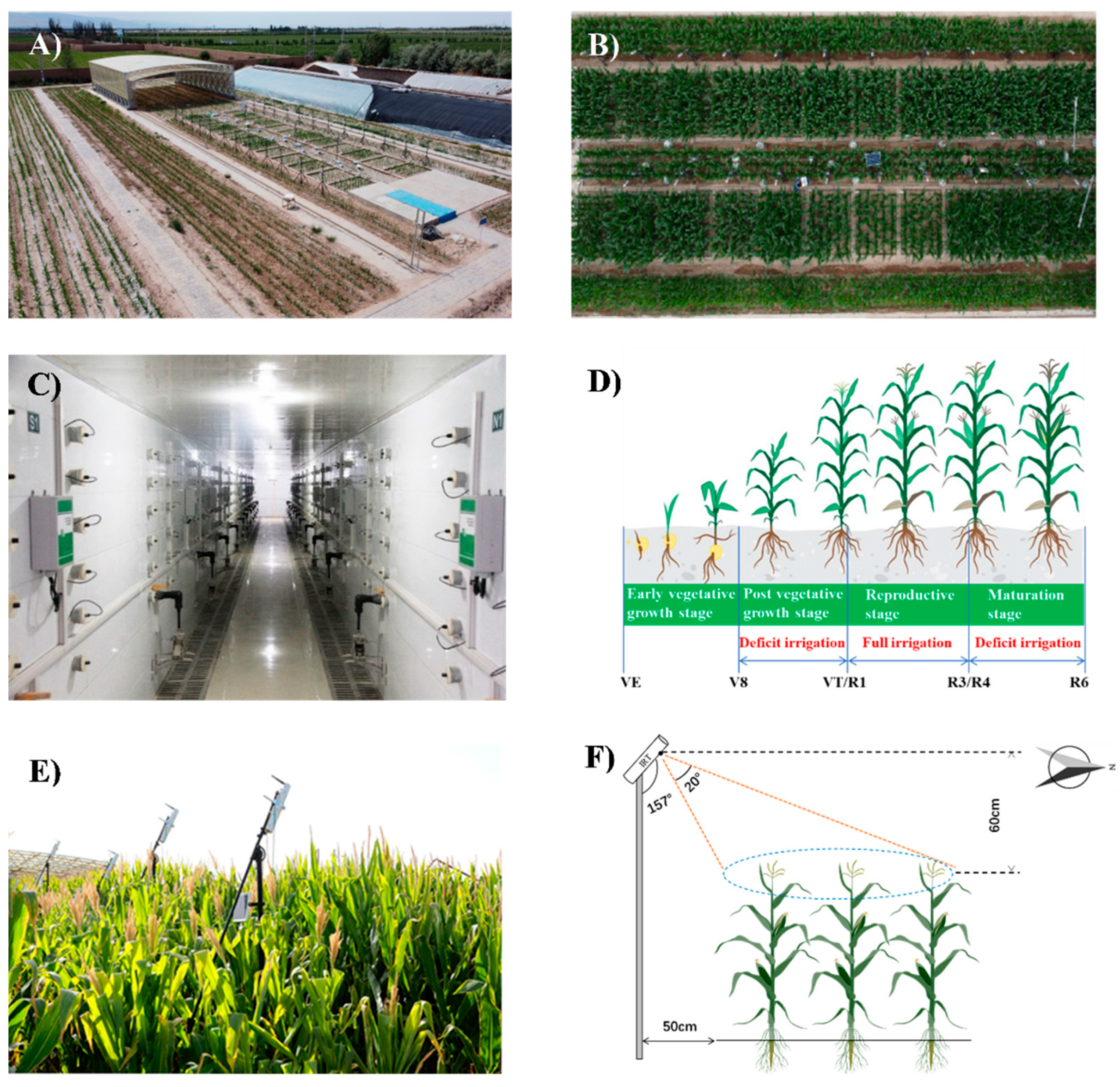
2.1. Experimental Area and Design

The experiment was conducted in the Shiyanghe Experimental Station of China Agricultural University from 1 May to 25 September in 2020. The experimental station is in Liangzhou District, Wuwei City, Gansu Province, China (37°51′ N, 102°52′ E, altitude 1581 m). The area is located in a typical temperate continental climate (inland arid desert climate), with abundant light and heat resources, according to the Koppen–Geiger classification. Annual sunshine hours exceed 3000 h, solar radiation is 5694 MJ m−2, the frost-free stage is more than 150 d, the average yearly temperature is 8 °C, and there is an annual sum of 3550 growing degree days (0 °C as base temperature). Water resources in this area are relatively scarce, with an average annual precipitation of 164 mm, average annual pan evaporation of ~2000 mm, and groundwater table below 25 m depth [39].
The experiment was carried out under a mobile electric rain-shelter facility of about 600 m2, where the 24 experimental plots consisted of hydrologically isolated non-weighing lysimeters (Figure 1A–C). Each lysimeter has an area of 5.6 m2 (2.8 m × 2 m) and a depth of 1.6 m. Each wall of the lysimeter is built of concrete, and sandy loam is backfilled and compacted. Therefore, the texture of lysimeter soil is relatively uniform and the physical and chemical properties are comparable. The average dry bulk density of the soil at a depth of 0–100 cm is 1.59 g cm−3, and the average field capacity is 0.28 cm3 cm−3.
The experiment set up two water (full irrigation, W1, and regulated deficit irrigation, W2) and two salt treatments (salt-free, S1 and soil salt content 2‰, S2) for two genotypes (Zhengdan 958, ZD958 and Xianyu 335, XY335). There were four treatments for each genotype, denoted as W1S1, W2S1, W1S2, and W2S2, with three replicates for each treatment (n = 3)—a total of 24 experimental plots, corresponding to 24 lysimeters. The experimental plots were arranged entirely randomly. Maize seeds were sown under the plastic film through 5.0 cm diameter holes at a planting density of 55 plants per plot. Two maize genotypes (ZD958 and XY335) were selected because they are widely planted in China. ZD958 and XY335 were sown on 1 May and 5 May and harvested between 23 and 25 September. The maize growth stage in this experiment was divided into the vegetative growth and the reproductive growth stage, with reference to Abendroth et al. [40]. It was also subdivided into four stages: early vegetative growth (VE–V8), late vegetative growth (V stage, V8–VT), reproductive stage (R stage, R1–R3), and maturation stage (M stage, R4–R6). The V stage of ZD958 was from 22 June to 21 July, the R stage from 22 July to 11 August, and the M stage from 12 August to 23 September. The V stage of XY335 was from 25 June to 24 July, the R stage from 25 July to 14 August, and the M stage from 15 August to 25 September. Corresponding water and salt treatments were carried out during each growth stage, as seen in Figure 1D.
The two water treatments were growth stage-based, where 100/100 and 65/80 ET means that the irrigation amount was the proportion of crop water requirements (ET) during the late vegetative growth (V stage, V8–VT) and maturation stage (M stage, R4–R6). The irrigation amount for the full irrigation treatment was a function of predicted crop ET and adjusted as needed for measured soil water deficits to maintain the soil water content, SWC, within the readily available water range in the active root zone. Water use was estimated using FAO-56 dual crop coefficient methodology with basal crop coefficients adjusted for measured crop canopy growth and senescence to meet water requirements [41]. Deficit irrigation was applied, with a target of 65% and 80% of maximum water use during the late vegetative and maturation periods, respectively [40]. Water was applied through a surface drip irrigation system about every 10 days. Salt treatment, 2‰, was achieved by irrigating NaCl salt water to the soil in the early vegetative and mid-vegetative stages, respectively. The total nitrogen applied to the maize was 262 kg ha−1, and it was treated with herbicides, abamectin, and acetamiprid, according to the recommended dosage, to prevent pests and diseases.
The meteorological data were obtained from the automatic meteorological station (Hobo, Onset Computer Corp, Bourne, MA, USA). The monitoring data mainly included solar radiation, air temperature, relative humidity, wind speed, precipitation, etc. Table 1 showed the key meteorological parameters for the entire growing season and the study period in 2020.

2.2. Canopy Temperature and CWSI Calculation

Infrared thermometers (SapIP-IRT, Dynamax Co., Houston, TX, USA) were used to monitor the continuous canopy temperature (Tc) of maize (Figure 1E). The field of view of IRT was 20° and the accuracy was ±0.5 °C. The IRTs were installed on telescopic poles at an angle of 23° on the horizon to ensure that the crop canopy was mainly in the field of view, thereby avoiding the influence of soil temperature. The schematic diagram of the canopy temperature monitoring using the IRT sensor was shown in Figure 1F. The IRTs were kept at the height of 0.6 m above the top of the canopy throughout the growing season (adjusted twice a week owing to the change in plant height during the vegetative growth stage). The viewing area of the IRTs was approximately 0.23 m2. The experiment continuously monitored the maize Tc in real-time from 22 June 2020 to 5 September 2020, with an average temperature interval of 30 min. The data was processed by the three-step moving average formula and then used for data analysis and baseline establishment.
The CWSI was computed using the difference between a measured canopy and air temperatures (dTm) and the lower (dTLL) and upper (dTUL) limits of canopy–air temperature difference. The last two values denote non-water-stressed and non-transpiring conditions, respectively:
CWSI = ( dT m dT LL ) ( dT UL dT LL )
Based on the method of Idso et al. [18], dTLL and dTUL were calculated as linear functions of atmospheric vapor pressure deficit (VPD) and vapor pressure gradient (VPG), respectively.
dT LL = m × VPD + b
dT UL = m × VPG + b
VPD = e s ( T a ) e a
e s ( T a ) = 0.6108 × EXP ( 17.27 × T a T a + 237.3 )
e a = e s ( T a ) × ( RH 100 )
where m and b are the slope and intercept of the linear equation, respectively; dTLL–VPD and dTUL–VPG relationships are known as non-water-stressed baseline (NWSB) and non-transpiring baseline (NTB), respectively; VPG is the difference between the air-saturated water vapor pressure at temperature Ta and the air-saturated water vapor pressure at temperature Ta + b; es(Ta) is the saturated vapor pressure (kPa) at the air temperature Ta; ea is the actual vapor pressure (kPa); Ta is the air temperature (°C), and RH is the relative humidity. We selected data from the end of June to the beginning of September with no rainfall (without the impact of shelters) to compute the CWSI.
Three to four typical days in the V, R, and M stages of ZD958 and XY335 were chosen to calculate dTLL and VPD based on the Tc measured in the W1S1 treatment under fully irrigated conditions and with the temperature and humidity monitored by the weather station. The line part of the relationship between dTLL and VPD was obtained and regarded as the NWSB of maize. We selected four hours of the relationship between 10:00–14:00 between dTLL and VPD, which was similar to Taghvaeian et al. [42], to develop NWSB based on the linear part the dTLL-vs-VPD curve.
To investigate the seasonality of maize CWSI and its response to irrigation management in different growth stages, the dTLL of each growth stage was obtained according to the NWSB established in the V, R, and M stages. According to the suggestion of Gardner et al. [33], using a constant dTUL value to estimate CWSI did not introduce significant errors, so the constant of 5 °C was used for dTUL [43,44]. In this way, seasonal variations of CWSI for each treatment of ZD958 and XY335 in different growth stages were determined.

2.3. Gas Exchange and Water Potential Measurements

One day before the in situ leaf gas exchange measurement, two adjacent and similar maize plants were selected, one for measuring the predawn leaf water potential and the other for measuring the gas exchange and midday leaf water potential. Leaf gas exchange was measured using a portable photosynthesis system (LI-6400, LICOR Biosciences, Lincoln, NE, USA), including stomatal conductance (gs), net photosynthetic rate (A), and other indicators. We selected the fully expanded leaf exposed to the sun at the vegetative stage and the third or fourth fully expanded leaf at the reproductive and maturation stage for measurement. All measurements were carried out between 10:00 and 11:30 (local standard time) within two sunny days. ZD958 and XY335 were measured on 7 July and 10 July in stage V, 29 July, and 1 to 2 August in stage R, and 3 September in stage M, respectively. In all situations, measurements were taken on three different individuals of each treatment, and the leaf chamber parameters were set to be consistent with the surrounding environment.
The predawn leaf water potential (Ψpd) was measured using a pressure chamber (Model 1515D, PMS Instrument Company, Albany, OR, USA). After midday in situ gas exchange measurement each day, the same part of the leaves was collected to measure midday leaf water potential (Ψmd) using a pressure chamber within 5 min.

2.4. Measurement of Leaf Area Index, Effective Leaf Width, Biomass, Yield, and ET

Leaf area index (LAI) was measured by direct manual measurement. Two maize individuals were randomly selected from each plot, and the measurement was performed every 7–10 d. While measuring the length and width of each leaf, effective width (We) was measured, which was considered to be the diameter of the largest circle within the edge of the leaf and closely related to the size and shape of the leaf [45,46]. By accumulating the product of the length and width of each leaf and multiplying it by the corresponding proportional coefficient, the leaf area per individual was obtained, that is, the leaf area = Σ (length × maximum width × 0.75). LAI was obtained by multiplying the number of maize units per unit ground by the average unit leaf area.
Aboveground biomass (AGB) was measured on 8 July in the V stage, 11 August in the R stage, and 18 September in the M stage of maize. One plant was randomly selected from each plot for measurement and was divided into four parts: stems, leaves, ears, and fruits for bagging. They were dried for about 72 h (85 °C) until the weight no longer changed. Maize plants were harvested from 23 to 25 September. Grain yield (GY) was determined by weighing the dry mass after drying at 85 °C to a constant weight. The final yield was standardized to 15.5% seed moisture content (commercial yield standard).
The soil moisture content (SWC, cm3 cm−3) of 0–100 cm was monitored by a neutron probe (CPN-503, Hydroprobe, InstroTek, San Francisco, CA, USA), and supplementary measurements were taken before and after irrigation. There was no influence of precipitation during the whole growth stage. The crop water use (ET) was estimated according to the principle of soil water balance. Since the experiment used minor flow drip irrigation and a rain-out shelter facility, there was no deep leakage during the maize growth stage. ET can be adequately calculated from irrigation and changes in soil moisture content.

2.5. Data Analysis

The temperature differences ΔTc1, ΔTc2, and ΔTc3 between treatments denoted the differences of Tc between W2S1, W1S2, and W2S2 with W1S1, respectively. SPSS 20.0 software (IBM, Inc., New York, NY, USA) was used to analyze variance (ANOVA) and Tukey’s posthoc test for mean comparison. Linear regression analyzed the relationship between CWSI and crop physiology, growth, water use, and yield indicators. To test whether there was a difference between XY335 and ZD958, the application “Compare Linear Fitting Parameters and Data Set” in OriginPro 2021 (OriginLab Software, Inc., Northampton, MA, USA) was used to analyze covariance (ANCOVA). The null expectation (H0) was that the slope of the regression (or intercept) would not deviate significantly between genotypes. Regression lines were fit for each genotype when either the slopes or intercepts of the relationship between a trait and CWSI were significantly different between genotypes. Regressions lines were fit across all genotypes when both the slopes and intercepts of the relationship between a trait and CWSI were not significantly different between genotypes. To avoid Type II errors, a probability level of p = 0.1 was set as the threshold for significance.

3. Results

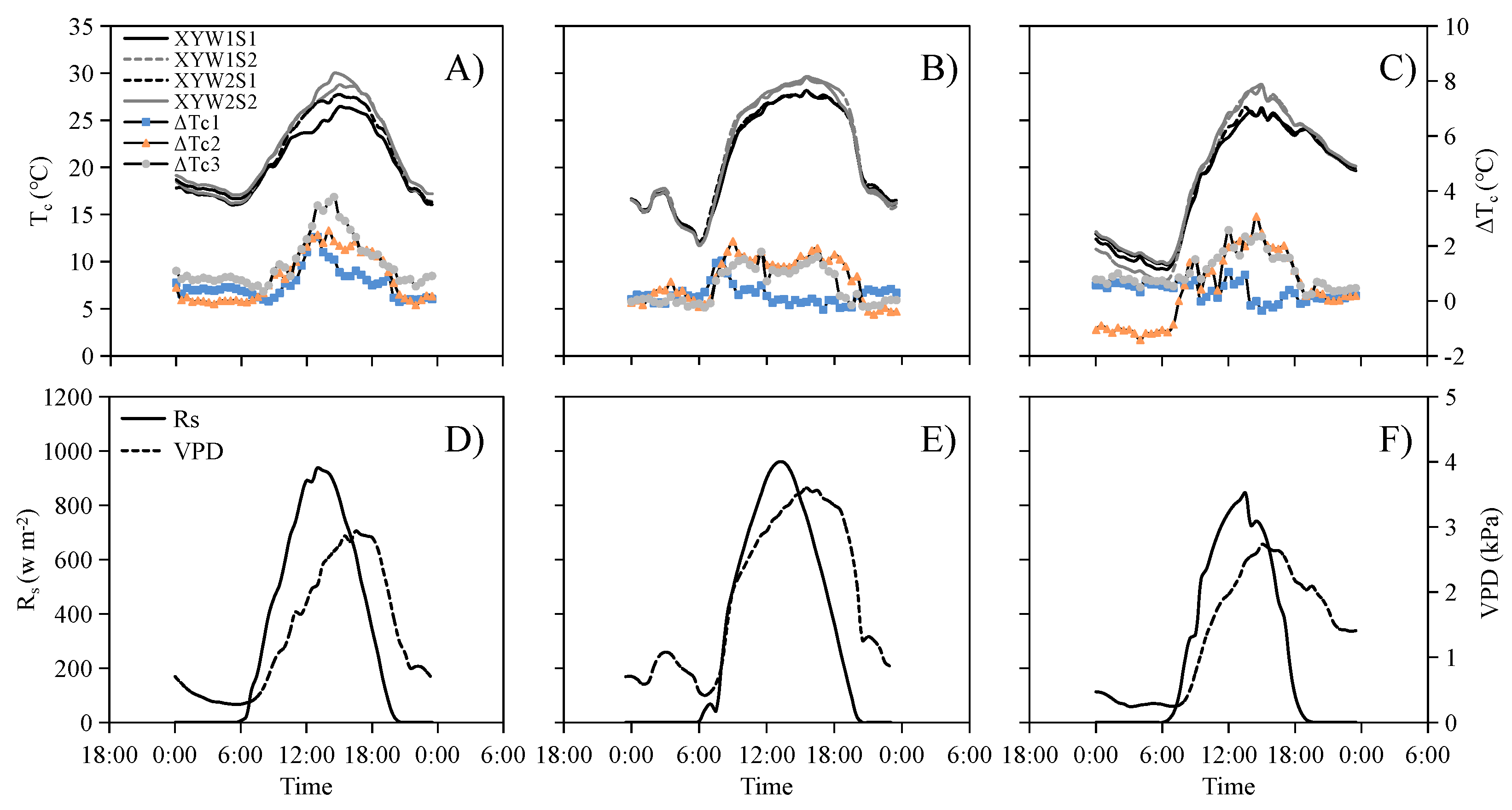
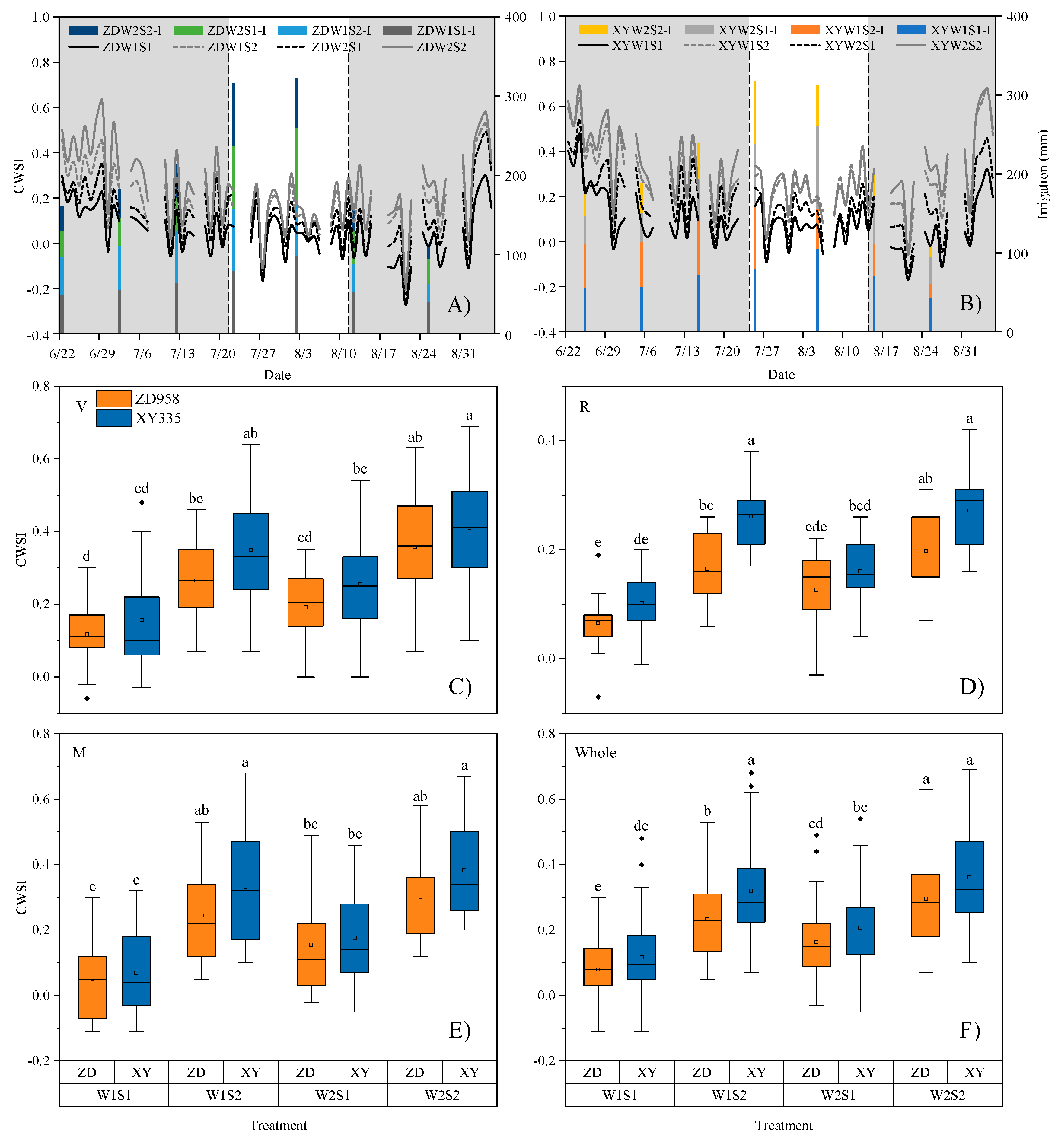
3.1. Tc Can Characterize the Degree of Water and Salt Stress on Maize

Figure 2 showed the diurnal variation in Tc of XY335 under four different treatments, as well as the variation in the temperature difference between the stress treatments and the control treatment with the first stage of water deficit (V stage, Figure 2A), rehydration (R stage, Figure 2B), and the second stage of water deficit (M stage, Figure 2C). In stage V (Figure 2A), ΔTc1, ΔTc2, and ΔTc3 all continued to increase from around 8 a.m. and reached their maximum values of 2.7, 2.9, and 4.3 °C between 12:00 and 15:00, respectively. With the decrease in VPD and solar radiation, these differences gradually decreased or even disappeared. The daily courses of ΔTc1, ΔTc2, and ΔTc3 indicated that the best time for Tc to characterize the degree of maize stress was 12:00–15:00 noon, and these two time points roughly coincided with the time when Rs and VPD reached their highest point (Figure 2D). This was because the demand for evaporation during this period was higher, and the response of crops to different stresses was more distinct. In the R stage (Figure 2B), the peak values of ΔTc1, ΔTc2, and ΔTc3 were 1.5, 2.2, and 1.8 °C, respectively. ΔTc1 and ΔTc3 decreased dramatically after rewatering, and ΔTc2 also decreased to a certain extent, indicating that the Tc of different stress treatments after rewatering could better characterize the elimination or alleviation of stress. The daily variation patterns of ΔTc1, ΔTc2, and ΔTc3 in the M stage (Figure 2C) were like those in the V stage, but the fluctuation was more remarkable, which might be related to the fluctuation of Rs during the day (Figure 2D,F). The average value of ΔTc1 between 12:00 and 15:00 was 0.5 °C, which was due to the mitigation of the water deficit in the second stage, while the ΔTc2 and ΔTc3 of the salt treatment remained at a high level, with the average values of 1.9 and 2.0 °C, respectively. In short, Tc can better characterize the degree of water and salt stress on maize and can be used to develop a CWSI model.

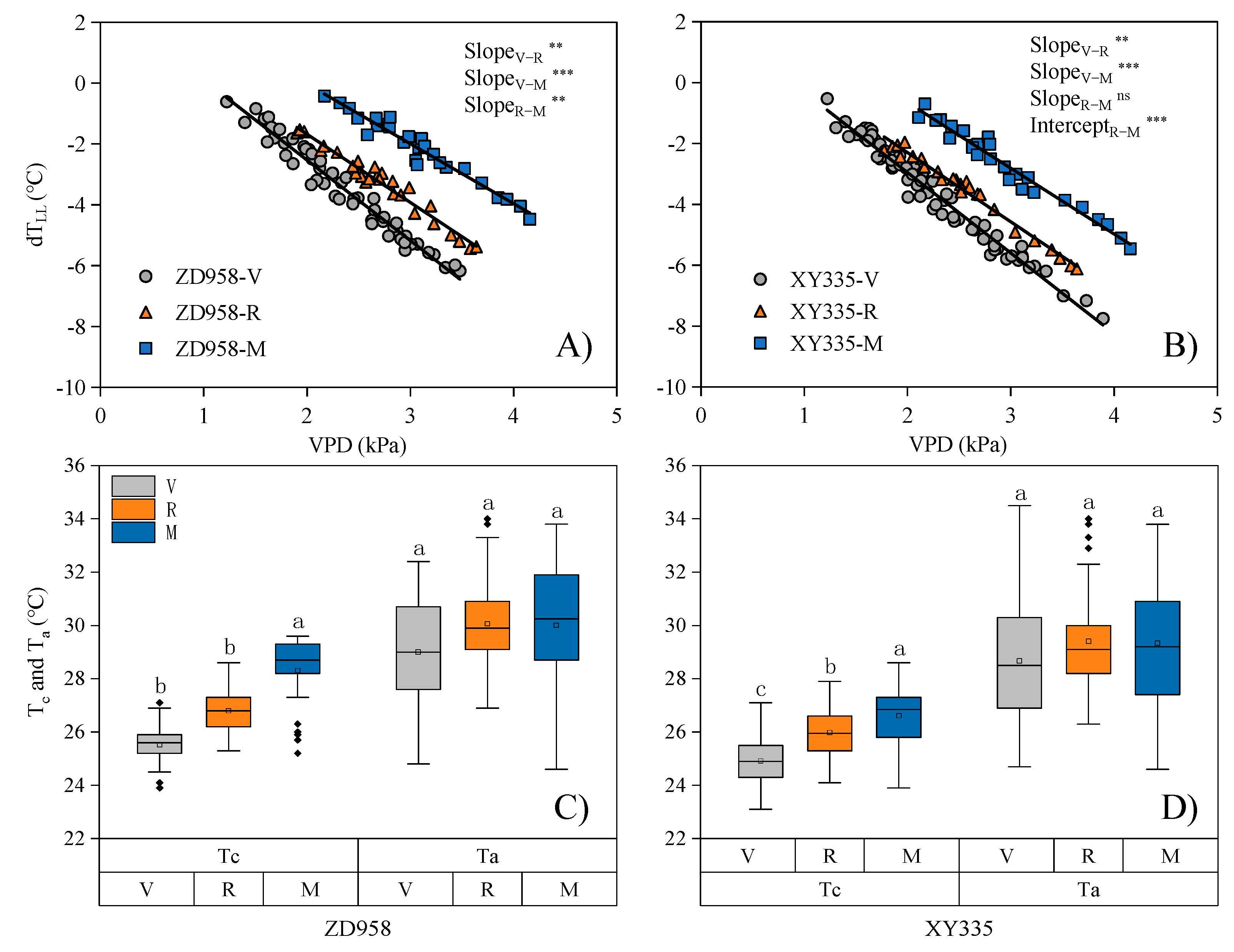
3.2. Growth Stage-Specific NWSBs Are Necessary for Establishing the CWSI Model

The slope and intercept of NWSB had changed dramatically as the growth stage of maize changed for both ZD958 and XY335 (Figure 3 and Table 2). There were significant differences between NWSB in each growth stage (that is, the slope of each growth stage in Figure 3 was significantly different). Therefore, we separately established NWSB for ZD958 and XY335 maize in the V, R, and M stages (Table 2). The absolute values of the NWSB slopes of both ZD958 and XY335 were V stage > R stage > M stage. However, we not only found that Tc increased significantly as the growth shifted from the V stage to the R stage, but also found that the increase in Ta during the same stage was negligible (Figure 3C,D), which led to an increase in dTLL under similar VPD changes and, at the same time, the slope of the NWSB become lower. As maize grew to the M stage, the Tc of maize still increased to varying degrees, while Ta was almost unchanged or slightly decreased, which might lead to a lower slope.

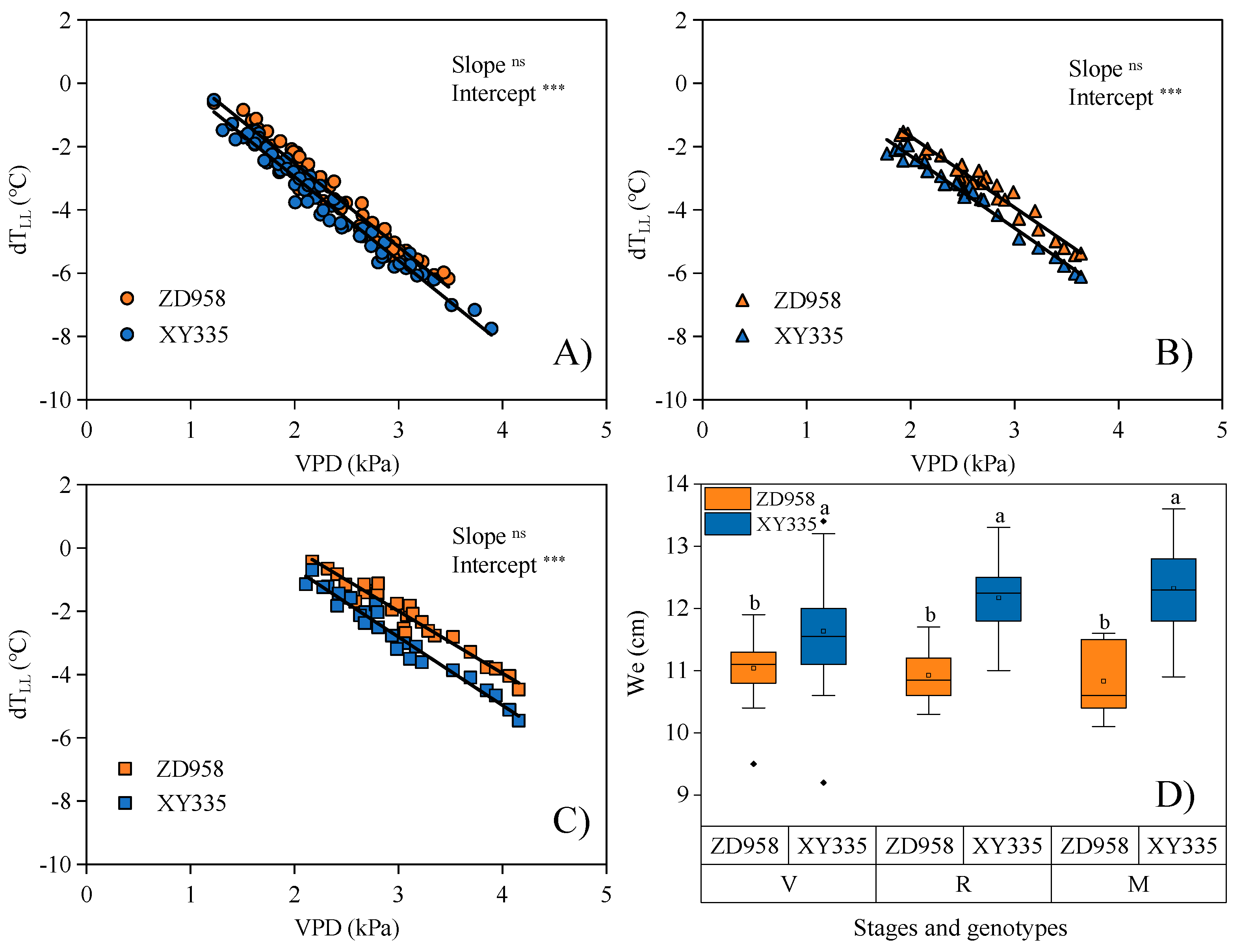
3.3. Significant Differences in NWSB Are Attributed to the Differences in Leaf Morphology between Maize Genotypes

In the V (Figure 4A), R (Figure 4B), and M stages (Figure 4C) of maize growth, there were no significant differences in the NWSB slopes of ZD958 and XY335. Because the NWSB slope reflects crop transpiration capacity, this indicated that the transpiration rates of ZD958 and XY335 were similar in each growth stage [50]. However, there were significant differences in the NWSB intercept between genotypes in each growth stage. The NWSB intercept of XY335 was smaller than that of ZD958, and the gap gradually increased with the growth of maize (Figure 4A–C). This suggested that the Tc of XY335 was lower than that of ZD958, and their Tc was different. Interestingly, we found that there were also significant differences at different growth stages in the We of the two genotypes. The We of XY335 were greater than that of ZD958, and this difference increased with the growth and development of maize (Figure 4D).
Compared with the previous NWSB developed for maize in areas with similar climatic conditions [30,42,43,47,48,49,51], the NWSB slopes and intercepts of the ZD958 and XY335 in this study were within the range of the existing NWSB slope (−1.79–3.35) and intercept (1.06–3.43), and the VPD range was also within the range of the previous NWSB (1.0–5.5 kPa). In stage M, the NWSB of XY335 in this study was almost the same as No. 1 and 2 [42,47] (Table 2). There was no significant difference in slopes between the NWSB of ZD958 and No. 1 and 2, but the intercepts were significantly different. This might be related to the more significant morphological difference of maize genotypes in ZD958 and No. 1 and 2 studies. NWSBs of XY335 and ZD958 were significantly different from No. 4 [32], which might be caused by significant differences in climatic conditions. In stage V, this study’s NWSB of ZD958 and XY335 was the same as that of No. 5 [48]. R2 was the same, and the slope was not significantly different, but the intercept was different. This was because the NWSB was also affected by relative humidity measurement location and equipment, and even the NWSB developed for maize in the same location also changed [43,49]. In short, the maize NWSB in this study was suitable for establishing the CWSI empirical model in this area.

3.4. CWSI Characterizes the Seasonal Dynamics of Maize under Water and Salt Stress

As shown in Figure 5A,B, the CWSI of each treatment of the two genotypes showed a “V”-shaped seasonal variation throughout the study stage, which resulted from the comprehensive response of CWSI to regulated deficit irrigation under salt conditions. Specifically, during the V stage, a moderate water deficit was carried out on the maize, and the irrigation amount was 65% of the fully irrigated ET. At the same time, the salinity of the saline soil increased to 2‰, which corresponded to higher CWSI after treatment. Because maize was under severe water and salt stress in the V stage, the response of each treatment to irrigation was also evident. Within a few days after irrigation, each treatment narrowed the gap with the CWSI of W1S1 treatment. With rewatering in the R stage, the irrigation amount was 100% of the fully irrigated ET, the CWSI of each treatment dropped to a lower level, and water and salt stresses on maize were alleviated significantly. With a water deficit in the M stage again, the irrigation amount was 80% of the fully irrigated ET, and the CWSI value of each treatment began to increase again until it reached nearly 0.7 at the end of the study (Figure 5). However, this significant increase in CWSI appeared as maize reached physiological maturity, and this increase seemed to be related to the closure of stomata caused by leaf senescence, not just due to water and salt stress. The average CWSI value of each treatment in the V stage was the largest among the three growth stages, while the R stage was the smallest. There was a significant difference in the average CWSI of each treatment during the entire growth stage, and the relationship was: W2S2 > W1S2 > W2S1 > W1S1, and the patterns of two maize genotypes were consistent (Figure 5C–E). Therefore, CWSI can accurately characterize seasonal dynamics and degree of water and salt stress on maize, which has specific practical significance for guiding differentiated regulated deficit irrigation during crucial growth stages.

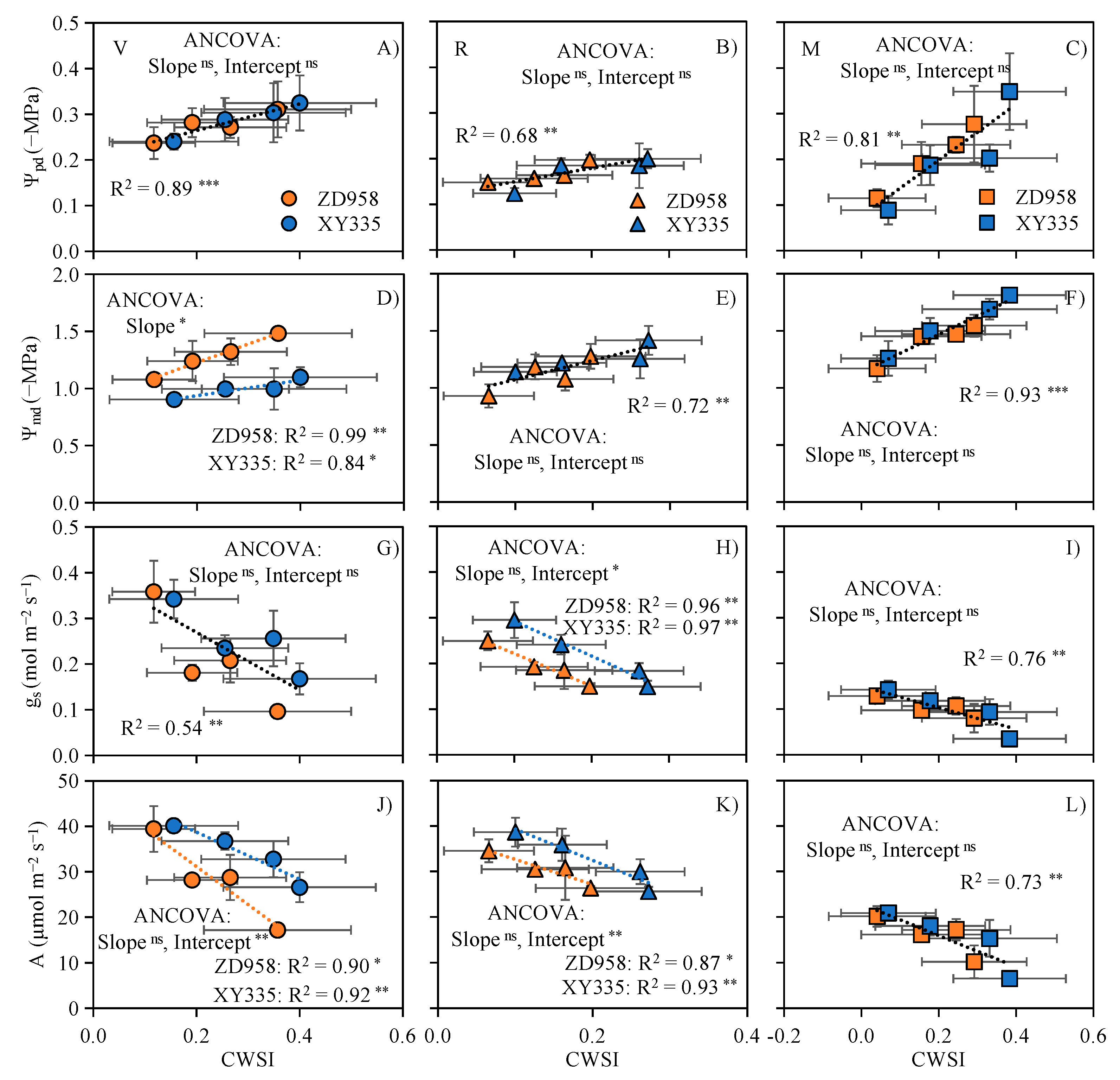
3.5. CWSI Can Diagnose the Physiological Variations of Maize under Water and Salt Stress

The relationships between Ψpd and Ψmd with CWSI were shown in Figure 6. The linear regression of Ψpd and CWSI with the two maize genotypes was more consistent in different growth stages, and the slope and intercept were not significantly different (Figure 6A–C). However, there was a significant difference between the linear regression of Ψmd and CWSI in stage V (Figure 6D). In the R and M stages, the CWSI of two maize genotypes had a significant linear correlation with Ψmd. As shown in Figure 6G–L, there was a significant linear correlation between gs and A with CWSI. In stage V, gs reached the maximum value of 0.35 mol m−2 s−1, equivalent to a CWSI close to 0.1. When the CWSI increased to about 0.4, the minimum gs value observed was lower than 0.1 mol m−2 s−1.

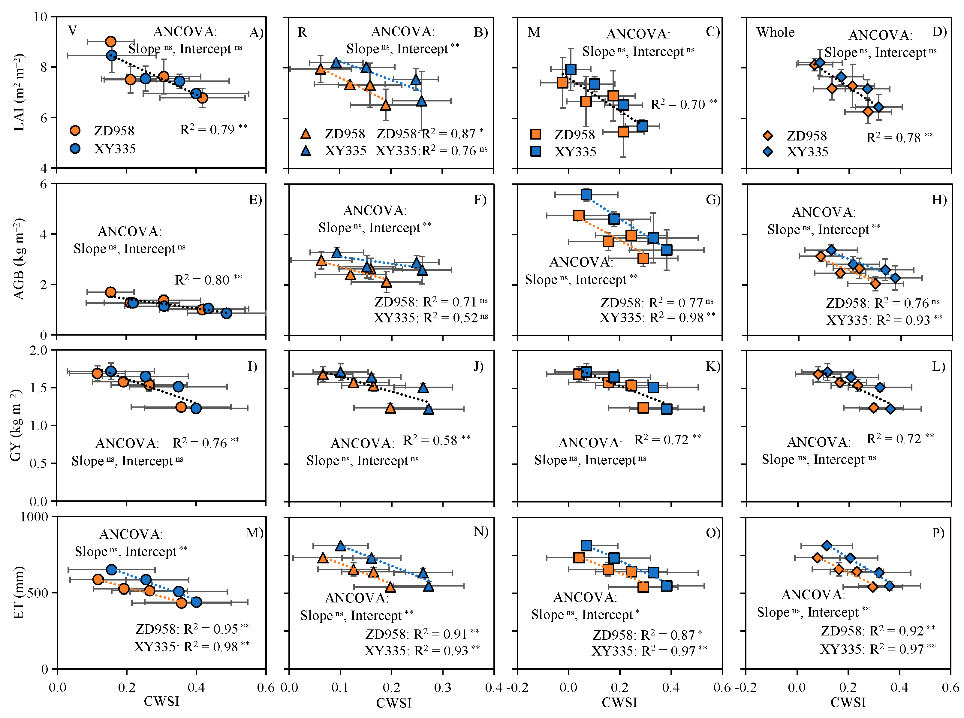
3.6. CWSI Can Predict Maize Growth, Yield, and Water Use under Water and Salt Stress

LAI and CWSI were all negatively correlated during the three growth stages of V, R, and M stages and the whole growth period (Figure 7A–D). Furthermore, during the V, M, and entire growth stages, the linear regressions of the two genotypes had no significant difference. The average LAI of the whole growth period decreased from ~8.2 m2 m−2 under no water stress to ~6.3 m2 m−2 under severe water stress. From Figure 7E–H, we found that AGB and CWSI were all negatively correlated across the growth stages. Additionally, there was no significant difference in the linear regression of the two genotypes of maize in the V stage (Figure 7E). The relationships between GY and ET with CWSI were shown in Figure 7I–P. There was a significant linear correlation between GY and ET with CWSI. Also, the linear regression between GY and CWSI had no significant difference between genotypes, which indicated that both GY and ET linearly decreased with CWSI, but the rate of decline in GY was equivalent. Maize yield decreased with the increase in average CWSI throughout the growing season (Figure 7L). We also found that GY can be better predicted in the V stage where the more severe plant water deficit (Figure 7I).

4. Discussion

Our results found that both Tc and CWSI can characterize the degree of water and salt stress on maize. Growth stage-specific NWSBs are necessary for establishing the CWSI model, and significant differences in NWSB are attributed to the differences in leaf morphology between maize genotypes. CWSI can diagnose and predict maize’s physiology, growth, and yield under combined water and salt stress.
As shown in Figure 2, Tc at 12:00–14:00 was the best time for capturing the most severe stress state experienced by crops, which was the same as in the previous study [47]. When establishing the CWSI model, significant differences in the growth stage of NWSB had been observed in many studies. Cui et al. [52] observed a similar phenomenon and found that the NWSB slope of summer maize was significantly different from jointing to tasseling stage, tasseling to milky ripening stage, and milky ripening to maturity stage. Ru et al. [50] determined the NWSB at different stages of greenhouse grapes and found that the absolute value of the slope of the NWSB was reduced in the flowering, fruit swelling, and ripening stages, respectively, 3.56, 2.51, and 1.97. Nielsen [53] reported a similar pattern that the NWSB of sunflower changed in the R6 stage. The NWSB in the V13–R5 stage had a steeper slope than the R6–R8 stage. They believed that this was caused by the gradual physiological maturity, the weakening of transpiration, and the increase in ear temperature after the sunflower entered the R6 stage. Gontia and Tiwari [54] established NWSB before and after heading in two consecutive growing seasons of wheat and found that the slope and intercept of the NWSB were significantly different. The expressions before heading were: dTLL = −1.75VPD − 1.26, and after heading: dTLL = −1.11VPD − 2.08; i.e., the slope of NWSB was less steep after heading. They attributed these to a greater operational canopy diffusion resistance of a wheat crop (capitulum) in the post-heading stage; therefore, for a given VPD increase, the post-heading stage had lower evaporative cooling and higher temperature than before heading. Some studies [30,55] made comparable explanations, and the same reason seemed to apply to maize crops. Here, compared with the V stage (before heading), ZD958 and XY335 had a smaller slope at the R stage (after heading) (Figure 3A,B). However, by comparing the changes in Tc and Ta of the two genotypes at different stages, we found that the increase in Tc was greater than that of Ta, resulting in a decrease in the slope of NWSB (Figure 3C,D), which was the same as the findings of Veysi et al. [23], who noted that the variation in baselines was related to the difference in weather between the beginning and the end of the growth stage. In short, reasons for the slope change of NWSB are more complicated and the slope of NWSB was less steep after heading. Therefore, a better choice for applying NWSB in the entire growth stage of maize crops was to distinguish the growth stages of the crop. Implementing the steeper NWSB of the V stage to the R and M stages with a smaller slope overestimated the CWSI of the R and M stages. Similar to our findings, Taghvaeian et al. [31] pointed out that this application might mislead growers to attribute higher temperatures to the water stress of the crops and to supplement water when the water in the root zone of the crop was not consumed to the critical point, resulting in a drop in water productivity. In addition, Zhang et al. [51] also pointed out that the mixed-use of NWSB could cause the reduction in CWSI’s recognition ability under different water stresses. Therefore, when establishing the CWSI empirical model, it needed to establish NWSB separately for different growth stages of maize.
The difference in leaf morphology between maize genotypes resulted in significant differences in NWSB (Figure 4). Idso et al. [56] found similar results that the water hyacinth NWSB of three different leaf sizes were different and their slopes were the same; but compared to the small leaf canopy, the intercept of the large leaf canopy was lower at 6 °C. Smith [57] showed that leaf temperature was mainly affected by leaf size. The leaf temperature of desert perennials with relatively large leaves was much lower than the air temperature, accompanied by a significant transpiration rate per unit leaf area. Therefore, differences and changes in leaf size of ZD958 and XY335 were likely to be the reason for the significant differences in their NWSB intercepts (Figure 4D). Different maize genotypes had different NWSB, limiting the broad application of the CWSI empirical model in irrigation management. However, many studies have shown that NWSB developed for different genotype crops of the same species (wheat, sunflower, and maize) with similar morphology might be very stable [31,53,56]. Therefore, in terms of actual production and management, if there are slight differences in the genotype morphology of crops grown on the same farm (for example, between different generations of the same product), there is no need to develop NWSB for each genotype to achieve the application of rapid CWSI.
CWSI can more accurately indicate the physiological health of crops through plant physiological indicators (such as Ψpd, Ψmd, gs, and A; Figure 6). Previous studies [58,59] confirmed that water potential could well reflect the stress levels experienced by plants, but there were still many difficulties in measuring water potential. The good relationships between CWSI and Ψpd and Ψmd in this study suggest that CWSI has the potential to replace water potential. Based on the relationship between CWSI with Ψpd and Ψmd, stress diagnosis by water potential can be shifted to CWSI. Similarly, Egea et al. [26] and Gonzalez-Dugo et al. [28] found that gs decreased linearly with the increase in CWSI in olive trees and apricot trees, respectively. Egea et al. [26] also reported that, compared with water potential, CWSI had a better correlation with gs. They believed that this was consistent with the theoretical basis of CWSI, described by Maes and Steppe [17] and Jones [60]; that is, control of stomata on transpiration rate under water stress is the main reason driving the change of CWSI. However, we found that the relationships between Ψpd and Ψmd with CWSI seemed to be better than gs (Figure 6A–I), which was similar to Bellvert et al. [35]. They found, in nectarines, that the correlation between gs and CWSI was not always better than water potential. Overall, CWSI can diagnose the stress state of maize plants and be used as a diagnostic indicator of maize physiological stress in this region.
The excellent relationship between CWSI and LAI, AGB, and GY indicated that CWSI can predict the growth and production of maize under water and salt stress (Figure 7), which was similar to previous studies. Sezen et al. [61] found that the CWSI of red pepper increased from 0.2 to 0.7, and LAI dropped from the peak value of 3.5 m2 m−2 to ~1.5 m2 m−2. Kirnak et al. [62] also observed that the LAI of pumpkin decreased significantly as CWSI increased. This decrease in LAI was related to the increase in Tc and the decrease in transpiration [61]. Yazar et al. [48] found that, within the range of the seasonal average CWSI, the relationship between AGB and CWSI was linear. The saline–alkali environment affects plant growth and development by causing the physiological responses of reducing plant water potential and directly reducing the photosynthetic rate or affecting certain specific enzymes or metabolic processes [63]. Previous studies found a significant correlation between CWSI, plant yield, and water use [64,65,66,67]. In addition, some studies believed that GY was more susceptible to water stress at the grain filling stage [68,69]. The relationship between GY and CWSI in the V stage was the best (Figure 7I–L), which was the same as Han et al. [49].

5. Conclusions

This study indicated that Tc could characterize the degree of water and salt stress on maize. There were significant differences in NWSB in different growth stages; thus, growth stage-specific NWSBs were necessary. Significant differences in NWSB were attributed to the differences in leaf morphology between maize genotypes. CWSI can characterize the seasonal dynamics of maize under water and salt stress. And CWSI can diagnose the physiological variations, growth, yield, and water use of maize under water and salt stress. Overall, CWSI can be used as a high-throughput phenotyping proxy for maize performance under combined water and salt stress.
Currently, measuring canopy temperature becomes more convenient and faster with the help of the rapid development of aerospace remote sensing imaging technology based on unmanned aerial vehicles and satellites [70]. Therefore, these insights presented here, which can expand the entire field to the regional range, will be valuable for predicting yield and improving water use efficiency.

Author Contributions

Experiment design: S.G. (Shujie Gu), Q.L. and R.D. Data analysis: S.G. (Shujie Gu), Q.L. and R.D. Contributed reagents/materials/analysis tools: S.G. (Shujie Gu), Q.L., S.G. (Shaoyu Gao), S.K., T.D. and R.D. Manuscript writing: S.G. (Shujie Gu), Q.L., S.G. (Shaoyu Gao), S.K., T.D. and R.D. All authors have read and agreed to the published version of the manuscript.

Funding

This work was supported by the National Natural Science Foundation of China (51790534 and 52179051) and the China Agriculture Research System of MOF and MARA (CARS-03).

Institutional Review Board Statement

Not applicable.

Informed Consent Statement

Not applicable.

Data Availability Statement

The data presented in this study are available on request from the corresponding author.

Acknowledgments

The authors would like to express their gratitude to the funding agencies, the editor and reviewers for leveraging the quality of this work, and the students who participated in the fieldwork and laboratory work.

Conflicts of Interest

The authors declare no conflict of interest.

References

  1. Alghory, A.; Yazar, A. Evaluation of crop water stress index and leaf water potential for deficit irrigation management of sprinkler-irrigated wheat. Irrig. Sci. 2019, 37, 61–77. [Google Scholar] [CrossRef]
  2. Kang, S.; Hao, X.; Du, T.; Tong, L.; Su, X.; Lu, H.; Li, X.; Huo, Z.; Li, S.; Ding, R. Improving agricultural water productivity to ensure food security in China under changing environment: From research to practice. Agric. Water Manag. 2017, 179, 5–17. [Google Scholar] [CrossRef]
  3. Cakir, R. Effect of water stress at different development stages on vegetative and reproductive growth of corn. Field Crop. Res. 2004, 89, 1–16. [Google Scholar] [CrossRef]
  4. Jiang, J.; Feng, S.; Ma, J.; Huo, Z.; Zhang, C. Irrigation management for spring maize grown on saline soil based on SWAP model. Field Crop. Res. 2016, 196, 85–97. [Google Scholar] [CrossRef]
  5. Hu, Y.; Burucs, Z.; von Tucher, S.; Schmidhalter, U. Short-term effects of drought and salinity on mineral nutrient distribution along growing leaves of maize seedlings. Environ. Exp. Bot. 2007, 60, 268–275. [Google Scholar] [CrossRef]
  6. Yuan, C.; Feng, S.; Huo, Z.; Ji, Q. Effects of deficit irrigation with saline water on soil water-salt distribution and water use efficiency of maize for seed production in arid Northwest China. Agric. Water Manag. 2019, 212, 424–432. [Google Scholar] [CrossRef]
  7. Jones, H.G. Plants and Microclimate: A Quantitative Approach to Environmental Plant Physiology; Cambridge University Press: New York, NY, USA, 2014. [Google Scholar]
  8. Ben-Gal, A.; Agam, N.; Alchanatis, V.; Cohen, Y.; Yermiyahu, U.; Zipori, I.; Presnov, E.; Sprintsin, M.; Dag, A. Evaluating water stress in irrigated olives: Correlation of soil water status, tree water status, and thermal imagery. Irrig. Sci. 2009, 27, 367–376. [Google Scholar] [CrossRef]
  9. Gollan, T.; Turner, N.C.; Schulze, E.D. The responses of stomata and leaf gas exchange to vapour pressure deficits and soil water content III. In the sclerophyllous woody species Nerium oleander. Oecologia 1985, 65, 356–362. [Google Scholar] [CrossRef]
  10. Ding, R.; Kang, S.; Zhang, Y.; Hao, X.; Tong, L.; Li, S. A dynamic surface conductance to predict crop water use from partial to full canopy cover. Agric. Water Manag. 2015, 150, 1–8. [Google Scholar] [CrossRef]
  11. Jones, H.G. Plant water relations and implications for irrigation scheduling. Acta Horticul. 1990, 278, 67–76. [Google Scholar] [CrossRef]
  12. Ballester, C.; Jimenez-Bello, M.A.; Castel, J.R.; Intrigliolo, D.S. Usefulness of thermography for plant water stress detection in citrus and persimmon trees. Agric. Forest Meteorol. 2013, 168, 120–129. [Google Scholar] [CrossRef]
  13. Zhu, J.; Bo, X.; Liu, L. Improved protocol for the in situ measurement of water potential of plants with a thermocouple psychrometer. Chin. Bull. Bot. 2013, 48, 531–539, (in Chinese with English abstract). [Google Scholar]
  14. Agam, N.; Cohen, Y.; Berni, J.A.J.; Alchanatis, V.; Kool, D.; Dag, A.; Yermiyahu, U.; Ben-Gal, A. An insight to the performance of crop water stress index for olive trees. Agric. Water Manag. 2013, 118, 79–86. [Google Scholar] [CrossRef]
  15. Kullberg, E.G.; Dejonge, K.C.; Chavez, J.L. Evaluation of thermal remote sensing indices to estimate crop evapotranspiration coefficients. Agric. Water Manag. 2017, 179, 64–73. [Google Scholar] [CrossRef] [Green Version]
  16. Hsiao, T.C. Plant responses to water stress. Annu. Rev. Plant. Biol. 1973, 24, 519–570. [Google Scholar] [CrossRef]
  17. Maes, W.H.; Steppe, K. Estimating evapotranspiration and drought stress with ground-based thermal remote sensing in agriculture: A review. J. Exp. Bot. 2012, 63, 4671–4712. [Google Scholar] [CrossRef] [Green Version]
  18. Idso, S.B.; Jackson, R.D.; Pinter, P.J.; Reginato, R.J.; Hatfield, J.L. Normalizing the stress-degree-day parameter for environmental variability. Agric. Meteorol. 1981, 24, 45–55. [Google Scholar] [CrossRef]
  19. Jackson, R.D.; Idso, S.B.; Reginato, R.J.; Pinter, P.J. Canopy temperature as a crop water stress indicator. Water Resour. Res. 1981, 17, 1133–1138. [Google Scholar] [CrossRef]
  20. Argyrokastritis, I.G.; Papastylianou, P.T.; Alexandris, S. Leaf water potential and crop water stress index variation for full and deficit irrigated cotton in Mediterranean conditions. Agric. Agric. Sci. Procedia 2015, 4, 463–470. [Google Scholar] [CrossRef] [Green Version]
  21. Fitriyah, A.; Fatikhunnada, A.; Okura, F.; Nugroho, B.D.A.; Kato, T. Analysis of the drought mitigated mechanism in terraced paddy fields using CWSI and TVDI indices and hydrological monitoring. Sustainability 2019, 11, 6897. [Google Scholar] [CrossRef] [Green Version]
  22. O’Shaughnessy, S.A.; Evett, S.R.; Colaizzi, P.D.; Howell, T.A. A crop water stress index and time threshold for automatic irrigation scheduling of grain sorghum. Agric. Water Manag. 2012, 107, 122–132. [Google Scholar] [CrossRef] [Green Version]
  23. Veysi, S.; Naseri, A.A.; Hamzeh, S.; Bartholomeus, H. A satellite based crop water stress index for irrigation scheduling in sugarcane fields. Agric. Water Manag. 2017, 189, 70–86. [Google Scholar] [CrossRef]
  24. Yuan, G.; Luo, Y.; Sun, X.; Tang, D. Evaluation of a crop water stress index for detecting water stress in winter wheat in the North China Plain. Agric. Water Manag. 2004, 64, 29–40. [Google Scholar] [CrossRef]
  25. Bellvert, J.; Zarco-Tejada, P.J.; Marsal, J.; Girona, J.; Gonzalez-Dugo, V.; Fereres, E. Vineyard irrigation scheduling based on airborne thermal imagery and water potential thresholds. Aust. J. Grape Wine Res. 2016, 22, 307–315. [Google Scholar] [CrossRef] [Green Version]
  26. Egea, G.; Padilla-Diaz, C.M.; Martinez-Guanter, J.; Fernandez, J.E.; Perez-Ruiz, M. Assessing a crop water stress index derived from aerial thermal imaging and infrared thermometry in super-high density olive orchards. Agric. Water Manag. 2017, 187, 210–221. [Google Scholar] [CrossRef] [Green Version]
  27. Gonzalez-Dugo, V.; Zarco-Tejada, P.J.; Fereres, E. Applicability and limitations of using the crop water stress index as an indicator of water deficits in citrus orchards. Agric. For. Meteorol. 2014, 198, 94–104. [Google Scholar] [CrossRef]
  28. Gonzalez-Dugo, V.; Lopez-Lopez, M.; Espadafor, M.; Orgaz, F.; Testi, L.; Zarco-Tejada, P.; Lorite, I.J.; Fereres, E. Transpiration from canopy temperature: Implications for the assessment of crop yield in almond orchards. Eur. J. Agron. 2019, 105, 78–85. [Google Scholar] [CrossRef]
  29. Jackson, S.H. Relationships between normalized leaf water potential and crop water stress index values for acala cotton. Agric. Water Manag. 1991, 20, 109–118. [Google Scholar] [CrossRef]
  30. Idso, S.B. Non-water-stressed baselines: A key to measuring and interpreting plant water stress. Agric. Meteorol. 1982, 27, 59–70. [Google Scholar] [CrossRef]
  31. Taghvaeian, S.; Comas, L.; Dejonge, K.C.; Trout, T.J. Conventional and simplified canopy temperature indices predict water stress in sunflower. Agric. Water Manag. 2014, 144, 69–80. [Google Scholar] [CrossRef]
  32. Irmak, S.; Haman, D.Z.; Bastug, R. Determination of crop water stress index for irrigation timing and yield estimation of corn. Agron. J. 2000, 92, 1221–1227. [Google Scholar] [CrossRef]
  33. Gardner, B.R.; Nielsen, D.C.; Shock, C.C. Infrared thermometry and the crop water stress index. I. History, theory, and baselines. J. Prod. Agric. 1992, 5, 462–466. [Google Scholar] [CrossRef]
  34. Aladenola, O.; Madramootoo, C. Response of greenhouse-grown bell pepper (Capsicum annuum L.) to variable irrigation. Can. J. Plant Sci. 2014, 94, 303–310. [Google Scholar] [CrossRef]
  35. Bellvert, J.; Marsal, J.; Girona, J.; Gonzalez-Dugo, V.; Fereres, E.; Ustin, S.L.; Zarco-Tejada, P.J. Airborne thermal imagery to detect the seasonal evolution of crop water status in peach, nectarine and saturn peach orchards. Remote Sens. 2016, 8, 39. [Google Scholar] [CrossRef] [Green Version]
  36. Rud, R.; Cohen, Y.; Alchanatis, V.; Levi, A.; Brikman, R.; Shenderey, C.; Heuer, B.; Markovitch, T.; Dar, Z.; Rosen, C.; et al. Crop water stress index derived from multi-year ground and aerial thermal images as an indicator of potato water status. Precis. Agric. 2014, 15, 273–289. [Google Scholar] [CrossRef]
  37. Xu, J.; Lv, Y.; Liu, X.; Dalson, T.; Yang, S.; Wu, J. Diagnosing crop water stress of rice using infra-red thermal imager under water deficit condition. Int. J. Agric. Biol. 2016, 18, 565–572. [Google Scholar] [CrossRef]
  38. Zhang, L.; Zhang, G.; Meng, Y.; Chen, B.; Wang, Y.; Zhou, Z. Changes of Related Physiological Characteristics of Cotton Under Salinity Condition and the Construction of the Cotton Water Stress Index. China Agric. Sci. 2013, 46, 3768–3775, (in Chinese with English abstract). [Google Scholar]
  39. Fan, Y.; Ding, R.; Kang, S.; Hao, X.; Du, T.; Tong, L.; Li, S. Plastic mulch decreases available energy and evapotranspiration and improves yield and water use efficiency in an irrigated maize cropland. Agric. Water Manag. 2017, 179, 122–131. [Google Scholar] [CrossRef]
  40. Abendroth, L.J.; Elmore, R.W.; Boyer, M.J.; Marlay, S.K. Corn Growth and Development; Iowa State University: Ames, IA, USA, 2011. [Google Scholar]
  41. Allen, R.G.; Pereira, L.S.; Raes, D.; Smith, M. Crop Evapotranspiration: Guidelines for Computing Crop Water Requirements; FAO: Rome, Italy, 1998; FAO Irrigation and Drainage Paper No. 56. [Google Scholar]
  42. Taghvaeian, S.; Chavez, J.L.; Hansen, N.C. Infrared thermometry to estimate crop water stress index and water use of irrigated maize in northeastern Colorado. Remote Sens. 2012, 4, 3619–3637. [Google Scholar] [CrossRef] [Green Version]
  43. Dejonge, K.C.; Taghvaeian, S.; Trout, T.J.; Comas, L.H. Comparison of canopy temperature-based water stress indices for maize. Agric. Water Manag. 2015, 156, 51–62. [Google Scholar] [CrossRef]
  44. Steele, D.D.; Stegman, E.C.; Gregor, B.L. Field comparison of irrigation scheduling methods for corn. Trans. ASAE 1994, 37, 1197–1203. [Google Scholar] [CrossRef]
  45. Leigh, A.; Sevanto, S.; Close, J.D.; Nicotra, A.B. The influence of leaf size and shape on leaf thermal dynamics: Does theory hold up under natural conditions? Plant Cell Environ. 2017, 40, 237–248. [Google Scholar] [CrossRef]
  46. Mcdonald, P.G.; Fonseca, C.R.; Overton, J.M.; Westoby, M. Leaf-size divergence along rainfall and soil-nutrient gradients: Is the method of size reduction common among clades? Funct. Ecol. 2003, 17, 50–57. [Google Scholar] [CrossRef] [Green Version]
  47. Taghvaeian, S.; Chavez, J.L.; Bausch, W.C.; Dejonge, K.C.; Trout, T.J. Minimizing instrumentation requirement for estimating crop water stress index and transpiration of maize. Irrig. Sci. 2014, 32, 53–65. [Google Scholar] [CrossRef]
  48. Yazar, A.; Howell, T.A.; Dusek, D.A.; Copeland, K.S. Evaluation of crop water stress index for LEPA irrigated corn. Irrig. Sci. 1999, 18, 171–180. [Google Scholar] [CrossRef]
  49. Han, M.; Zhang, H.; Dejonge, K.C.; Comas, L.H.; Gleason, S. Comparison of three crop water stress index models with sap flow measurements in maize. Agric. Water Manag. 2018, 203, 366–375. [Google Scholar] [CrossRef]
  50. Ru, C.; Hu, X.; Wang, W.; Ran, H.; Song, T.; Guo, Y. Evaluation of the crop water stress index as an indicator for the diagnosis of grapevine water deficiency in greenhouses. Horticulturae 2020, 6, 864. [Google Scholar] [CrossRef]
  51. Zhang, L.; Niu, Y.; Han, W.; Liu, Z. Establishing method of crop water stress index empirical model of field maize. Trans. Chin. Soc. Agric. Mach. 2018, 49, 233–239, (in Chinese with English abstract). [Google Scholar]
  52. Cui, X.; Xu, L.; Yuan, G.; Wang, W.; Luo, Y. Crop water stress index model for monitoring summer maize water stress based on canopy surface temperature. Trans. Chin. Soc. Agric. Eng. 2005, 21, 22–24, (in Chinese with English abstract). [Google Scholar]
  53. Nielsen, D.C. Non water-stressed baselines for sunflowers. Agric. Water Manag. 1994, 26, 265–276. [Google Scholar] [CrossRef]
  54. Gontia, N.K.; Tiwari, K.N. Development of crop water stress index of wheat crop for scheduling irrigation using infrared thermometry. Agric. Water Manag. 2008, 95, 1144–1152. [Google Scholar] [CrossRef]
  55. Fritschen, L.J.; Bavel, C.H.M.V. Energy balance as affected by height and maturity of sudangrass. Agron. J. 1964, 56, 201–204. [Google Scholar] [CrossRef]
  56. Idso, S.B.; Reginato, R.J.; Clawson, K.L.; Anderson, M.G. On the stability of non-water-stressed baselines. Agric. For. Meteorol. 1984, 32, 177–182. [Google Scholar] [CrossRef]
  57. Smith, W.K. Temperatures of desert plants: another perspective on the adaptability of leaf size. Science 1978, 201, 614–616. [Google Scholar] [CrossRef] [PubMed]
  58. Meron, M.; Tsipris, J.; Orlov, V.; Alchanatis, V.; Cohen, Y. Crop water stress mapping for site-specific irrigation by thermal imagery and artificial reference surfaces. Precis. Agric. 2010, 11, 148–162. [Google Scholar] [CrossRef]
  59. O’Shaughnessy, S.A.; Evett, S.R.; Colaizzi, P.D.; Howell, T.A. Using radiation thermography and thermometry to evaluate crop water stress in soybean and cotton. Agric. Water Manag. 2011, 98, 1523–1535. [Google Scholar] [CrossRef]
  60. Jones, H.G. Stomatal control of photosynthesis and transpiration. J. Exp. Bot. 1998, 49, 387–398. [Google Scholar] [CrossRef]
  61. Sezen, S.M.; Yazar, A.; Dasgan, Y.; Yucel, S.; Akyildiz, A.; Tekin, S.; Akhoundnejad, Y. Evaluation of crop water stress index (CWSI) for red pepper with drip and furrow irrigation under varying irrigation regimes. Agric. Water Manag. 2014, 143, 59–70. [Google Scholar] [CrossRef]
  62. Kirnak, H.; Irik, H.A.; Unlukara, A. Potential use of crop water stress index (CWSI) in irrigation scheduling of drip-irrigated seed pumpkin plants with different irrigation levels. Sci. Hortic. 2019, 256, 108608. [Google Scholar] [CrossRef]
  63. Munns, R. Physiological processes limiting plant growth in saline soils: some dogmas and hypotheses. Plant Cell Environ. 1993, 16, 15–24. [Google Scholar] [CrossRef]
  64. Braunworth, W.S.; Mack, H.J. The possible use of the crop water-stress index as an indicator of evapotranspiration deficits and yield reductions in sweet corn. J. Am. Soc. Hortic. Sci. 1989, 114, 542–546. [Google Scholar]
  65. Colak, Y.B.; Yazar, A.; Colak, I.; Akca, H.; Duraktekin, G. Evaluation of crop water stress index (CWSI) for eggplant under varying irrigation regimes using surface and subsurface drip systems. Agric. Agric. Sci. Procedia 2015, 4, 372–382. [Google Scholar] [CrossRef] [Green Version]
  66. Nielsen, D.C. Scheduling irrigations for soybeans with the crop water-stress index (CWSI). Field Crop Res. 1990, 23, 103–116. [Google Scholar] [CrossRef]
  67. Smith, R.C.G.; Barrs, H.D.; Fischer, R.A. Inferring stomatal-resistance of sparse crops from infrared measurements of foliage temperature. Agric. For. Meteorol. 1988, 42, 183–198. [Google Scholar] [CrossRef]
  68. Egea, G.; Nortes, P.A.; Gonzalez-Real, M.M.; Baille, A.; Domingo, R. Agronomic response and water productivity of almond trees under contrasted deficit irrigation regimes. Agric. Water Manag. 2010, 97, 171–181. [Google Scholar] [CrossRef]
  69. Goldhamer, D.A.; Fereres, E. Establishing an almond water production function for California using long-term yield response to variable irrigation. Irrig. Sci. 2017, 35, 169–179. [Google Scholar] [CrossRef]
  70. Kang, J.; Hao, X.; Zhou, H.; Ding, R. An integrated strategy for improving water use efficiency by understanding physiological mechanisms of crops responding to water deficit: Present and prospect. Agric. Water Manag. 2021, 255, 107008. [Google Scholar] [CrossRef]
Figure 1. Overview of the experimental area and design. (A) a panoramic view of the mobile electric rain-shelter facility and experimental area; (B) two maize genotypes (XY335 and ZD958) are planted in 24 non-weighing lysimeters made of concrete, each with an area of 5.6 m2 (2.8 m × 2 m) and a depth of 1.6 m; (C) underground picture of 24 non-weighing lysimeters; (D) the schematic diagram of four growth stages of maize, and water treatments at each stage. In the figure, VE, V8, VT, R1, R3, R4, and R6 represent the stage of emergence, the 8th leaf, tasseling, silking, milky ripening, waxy ripening, and physiological maturation, respectively; and (E,F) the actual layout and schematic diagram of monitoring canopy temperature using the IRT sensor.
Remotesensing 13 04710 g001
Figure 2. Canopy temperature (Tc) and differences in Tc between treatments (ΔTc), (AC) for XY335 maize genotype and corresponding diurnal courses of solar radiation (Rs) and vapor pressure deficit (VPD), (DF). W1 and W2 are full and regulated deficit irrigation, and S1 and S2 salt-free and 2‰ soil salt content treatments, respectively. ΔTc1, ΔTc2, and ΔTc3 represent the temperature differences between W2S1, W1S2, and W2S2 with W1S1, respectively. The data are three typical days of the late vegetative stage (V stage, 7/1), (A,D), reproductive stage (R stage, 7/26), (B,E), and maturation stage (M stage, 8/28), (C,F), respectively.
Remotesensing 13 04710 g002
Figure 3. The relationships between lower limit of canopy-air temperature difference (dTLL) and vapor pressure deficit (VPD) during the late vegetative (V), reproductive (R), and maturation stages (M) for two maize genotypes, (A) ZD958 and (B) XY335, respectively. Average canopy (Tc) and air temperature (Ta) are presented during the V, R, and M stages for (C) ZD958 and (D) XY335, respectively. The slopes and intercepts among the three growth stages are compared by the ANCOVA test for (A) ZD958 and (B) XY335, respectively. For the box plot, the lower and upper bounds correspond to the first and third quartiles (interquartile range, IQR), the horizontal lines inside the boxes are the medians, the upper/lower whisker extends from the bound to the largest/smallest value no further than 1.5 × IQR from the bounds, and data beyond the end of the whiskers are plotted individually. The differences of Tc and Ta among different growth stages were analyzed by one-way ANOVA for ZD958 and XY335, respectively. Different letters denote significant differences (p < 0.05) by a Tukey’s posthoc test for means comparison. ns, no significant difference; **, p < 0.05; ***, p < 0.001.
Remotesensing 13 04710 g003
Figure 4. The relationships between lower limit of canopy-air temperature difference (dTLL) and vapor pressure deficit (VPD) for two maize genotypes (ZD958 and XY335) during (A) the late vegetative (V), (B) reproductive (R), and (C) maturation stages (M), respectively. (D) Average effective leaf width (We) is presented for two genotypes during three growth stages. The slopes and intercepts between two genotypes are compared by the ANOVA test during the V, R, and M stages, respectively. For the box plot, the lower and upper bounds correspond to the first and third quartiles (interquartile range, IQR), the horizontal lines inside the boxes are the medians, the upper/lower whisker extends from the bound to the largest/smallest value no further than 1.5 × IQR from the bounds, and data beyond the end of the whiskers are plotted individually. The differences in We between two genotypes are analyzed by one-way ANOVA during three growth stages. Different letters denote significant differences (p < 0.05) by a Tukey’s posthoc test for means comparison. ns, no significant difference; ***, p < 0.001.
Remotesensing 13 04710 g004
Figure 5. Seasonal variations in crop water stress index (CWSI) under different water and salt treatments for two maize genotypes, (A) ZD958 and (B) XY335, respectively, as well as average differences in CWSI during different and whole growth stages for two genotypes (CF). Vertical dotted lines in (A,B) separate the growth stages into the late vegetative (V), reproductive (R), and maturation stages (M), respectively. Grey areas indicate periods when all treatments are deficit-irrigated. Vertical bars on the separate ordinates represent the amount of irrigation for each treatment of each irrigation. W1 and W2 are full and regulated deficit irrigation, and S1 and S2 salt-free and 2‰ soil salt content treatments, respectively. For the box plot, the lower and upper bounds correspond to the first and third quartiles (interquartile range, IQR), the horizontal lines inside the boxes are the medians, the upper/lower whisker extends from the bound to the largest/smallest value no further than 1.5 × IQR from the bounds, and data beyond the end of the whiskers are plotted individually. The differences in CWSI between two genotypes are analyzed by one-way ANOVA during different growth stages, respectively. Different letters denote significant differences (p < 0.05) by a Tukey’s posthoc test for means comparison.
Remotesensing 13 04710 g005
Figure 6. The relationships between predawn leaf water potential (Ψpd), (AC), midday leaf water potential (Ψmd), (DF), stomatal conductance (gs), (GI), and net photosynthetic rate (A), (JL) with average crop water stress index (CWSI) during different growth stages of two maize genotypes (ZD958 and XY335). Regression lines are fit for each genotype when either the slopes or intercepts are significantly different, and across all genotypes when both the slopes and intercepts are not significantly different by the ANCOVA test. Values are means ± SD. ns, no significant difference; *, p < 0.1; **, p < 0.05; ***, p < 0.001.
Remotesensing 13 04710 g006
Figure 7. The relationships between leaf area index (LAI), (AD), aboveground biomass (AGB), (EH), grain yield (GY), (IL), and evapotranspiration (ET), (MP) with average crop water stress index (CWSI) during different growth stages of two maize genotypes (ZD958 and XY335). Regression lines are fit for each genotype when either the slopes or intercepts are significantly different, and across all genotypes when both the slopes and intercepts are not significantly different by the ANCOVA test. Values are means ± SD. ns, no significant difference; *, p < 0.1; **, p < 0.05.
Remotesensing 13 04710 g007
Table 1. Average daily meteorological variables for the whole growing season and the study period in 2020, respectively.
VariablesWhole Growth Season
(1 May–25 September)
Study Period
(22 June–5 September)
Mean air temperature (°C)19.5121.18
Maximum air temperature (°C)27.2229.19
Minimum air temperature (°C)12.0513.64
Vapor pressure (kPa)1.221.22
Minimum relative humidity (%)31.9134.48
Wind speed (m s−1)0.620.40
Solar radiation (W m−2)232.53232.82
Table 2. Slope, intercept, and other detailed parameters of non-water-stressed baselines’ (NWSBs) linear fitting reported in this study and previous maize studies.
No.SlopeInterceptGrowth
Stage
SourcesR2nVPD Range
(kPa)
VarietyLocationLatitude and LongitudeClimate
0−2.642.75VThis study0.96531.2~3.5ZD958Shiyanghe Experimental Station of China Agricultural University, Wuwei City, Gansu ProvinceLat. 37°52′ N, Long. 102°50′ EThe altitude is 1581 m, the average annual temperature is 8 °, and the average annual precipitation is 164 mm.
−2.242.81R0.96291.9~3.6
−1.963.89M0.95262.2~4.2
−2.622.27V0.97671.2~3.9XY335
−2.282.25R0.98261.8~3.6
−2.163.66M0.96262.1~4.2
1−1.902.73R3–R4Taghvaeian et al. [42]0.9861.5~4.0DKC52–60, Dekalb®Greeley, ColoradoLat. 40°46′ N, Long. 103°2′ WThe altitude is 1166 m, the average annual temperature is 11.5 °C, and the average annual precipitation is 373 mm.
2−1.993.04R–MTaghvaeian et al. [47]0.97121.5~4.0DKC52–59, Dekalb®Greeley, ColoradoLat. 40°26′ N, Long. 104°38′ WThe altitude is 1425 m, the average annual temperature is 11.5 °C, and the average annual precipitation is 373 mm.
3−1.973.11 Idso et al. [30]0.97970.8~4.5 Tempe, ArizonaLat. 33°25′ N, Long. 111°56′ WThe altitude is 430 m, the average annual temperature is 16.6 °C, and the average annual precipitation is 211 mm.
4−0.861.39R–MImark [32]0.92281.0~5.5var. AntbeyAntalya, TurkeyLat. 36°55’ N, Long. 34°55′ EThe altitude is 12 m, and the average annual precipitation is 1068 mm.
5−2.561.06VYazar et al. [48]0.93 1.2~3.2Pioneer 3245Bushland, TexasLat. 35°11′ N, Long. 102°06′ WThe altitude is 1170 m.
6−1.973.43 Han et al. [49]0.82 1.0~4.0 Greeley, ColoradoLat. 40°26′ N, Long. 104°38′ WThe altitude is 1427 m, the average annual temperature is 11.5 °C, and the average annual precipitation is 373 mm.
7−1.792.34 DeJonge et al. [43]0.97 DCK52–04, Dekalb®Greeley, ColoradoLat. 40°26′ N, Long. 104°38′ WThe altitude is 1427 m, the average annual temperature is 11.5 °C, and the average annual precipitation is 373 mm.
Note: the growth stages V, R, and M refer to the late vegetative (V8–VT), reproductive (R1–R3), and maturation stages (R4–R6), respectively, and R3–R4 refers to the third and fourth reproductive stages. R2, determination coefficient; n, sample size; and VPD, vapor pressure deficit.
Publisher’s Note: MDPI stays neutral with regard to jurisdictional claims in published maps and institutional affiliations.

