Improving the iGNSS-R Ocean Altimetric Precision Based on the Coherent Integration Time Optimization Model

Abstract

Improving the altimetric precision under the requirement of ensuring the along-track resolution is of great significance to the application of iGNSS-R satellite ocean altimetry. The results obtained by using the empirical integration time need to be improved. Optimizing the integration time can suppress the noise interference from different sources to the greatest extent, thereby improving the altimetric precision. The inverse relationship between along-track resolution and signal integration time leads to the latter not being infinite. To obtain the optimal combination of integral parameters, this study first constructs an analytical model whose precision varies with coherent integration time. Second, the model is verified using airborne experimental data. The result shows that the average deviation between the model and the measured precision is about 0.16 m. The two are consistent. Third, we apply the model to obtain the optimal coherent integration time of the airborne experimental scenario. Compared with the empirical coherent integration parameters, the measured precision is improved by about 0.1 m. Fourth, the verified model is extrapolated to different spaceborne scenarios. Then, the optimal coherent integration time and the improvement of measured precision under various conditions are estimated. It was found that the optimal coherent integration time of the spaceborne scene is shorter than that of the airborne scene. Depending on the orbital altitude and the roughness of the sea surface, its value may also vary. Moreover, the model can significantly improve the precision for low signal-to-noise ratios. The coherent integration time optimization model proposed in this paper can enhance the altimetric precision. It would provide theoretical support for the signal optimization processing and sea surface height retrieval of iGNSS-R altimetry satellites with high precision and high along-track resolution in the future.

1. Introduction

Accurately measured sea surface height (SSH) is one of the critical parameters of marine ecosystem monitoring, which is of paramount significance to applications such as fishery, oil drilling, and commercial navigation. Global navigation satellite systems reflectometry (GNSS-R) or the passive reflection and interference system (PARIS) can perform ocean altimetry as a passive remote sensing technique [1]. It has some unique advantages compared with the traditional tide gauge station and monostatic radar ocean altimetry. On the one hand, the receiver can capture multiple global navigation satellite system (GNSS) signals simultaneously, which increases the spatial coverage. On the other hand, as a novel bistatic passive remote sensing method, it has the characteristics of low cost, low power consumption, all-weather and high time revisit rate, which can make up for the shortcomings of the existing technology to a large extent. Since the technology was proposed, ground-based, air-based, and space-based altimetry experiments have been conducted successively to verify its feasibility [2,3,4].

Some signal processing techniques for GNSS-R ocean altimetry have been proposed. Conventionally, GNSS-R altimetry involves cross-correlating the reflected signals with the local replicas of the open navigation signals (cGNSS-R) [5]. The encrypted signal (e.g., P(Y)) has a broader bandwidth, which will bring a sharper autocorrelation function (ACF) and a higher range precision. With it, the reconstructed code GNSS-R (r-GNSS-R) altimetry improves the precision by reproducing the encrypted signals [6]. The interferometric altimetry (iGNSS-R) utilizes the full composite components of the direct signal to correlate with the reflected signal [5]. The partial interferometric GNSS-R (piGNSS-R) altimetry extracts a portion of the encrypted signal from the full composite components to obtain a sharper ACF, which is an extension of iGNSS-R [7]. Nevertheless, in the case of iGNSS-R and piGNSS-R, the loss of signal-to-noise ratio (SNR) caused by dual-channel noise is more severe than that of cGNSS-R, which leads to a two-fold improvement in precision only [8]. The SNR should be improved by increasing the signal processing time, as this will diminish the influence of thermal noise and speckle noise on altimetric precision [9]. However, a longer integration time corresponds to a longer specular point (SP) movement distance. Considering the moving speed of the sub-satellite point (km/s) and the size of the spatial footprint (~10 km), the actual inverted single height represents the average over the larger sea area which further reduces the along-track resolution [10]. The previous study has shown that in the spaceborne iGNSS-R altimetry scenario, in order to achieve an altimetric precision better than 20 cm, the signal processing time required for a single height retrieval is approximately 10 s, and the along-track spatial resolution is about 65 km [8]. If the iGNSS-R ocean altimetry with high precision and high along-track spatial resolution can be realized, it would provide critical data and information resources for small and medium scale ocean phenomena monitoring, high temporal and spatial resolution ocean gravity field model establishment, and other earth science research.

One of the data products of GNSS-R observation is the delay-Doppler maps (DDM). Fernando et al. detailed the corresponding relationship between the DDM and its spatial location [11]. The waveform corresponding to zero Doppler is extracted from the calibrated DDM waveform for GNSS-R code-delay altimetry, and the delay information of the reflected signal is extracted from this waveform. Commonly used retrieval algorithms include the peak point of the first derivative (DER), the peak of the waveform (MAX), and the half-power point (HALF) [8,12,13]. Obtaining the inversion delay requires correction of numerous parameters including the receiver and transmitter orbits, ionospheric errors, tropospheric errors, and antenna baseline offsets [14]. For the evaluation of the altimetry performance, Li et al. considered both the altimetric precision and the altimetric accuracy. Altimetric accuracy is primarily affected by systematic errors. The altimetric precision is mainly induced by the randomness of the received signal caused by thermal noise and speckle noise. Theoretically, the higher the SNR of the signal, the more accurate the SP delay information extracted from the waveform, and the better the altimetric precision [15].

It is possible to increase the altimetric precision by optimizing the payload and signal post-processing. Payload optimization includes increasing antenna gain, refining antenna pointing and receiver bandwidth, etc. [16,17]. For signal post-processing, one method to improve the altimetric precision is to increase the signal’s coherent integration time and incoherent average number. Both methods inhibit the noise introduced in different ways. The former is to suppress the thermal noise introduced at the receiver end, while the latter is to suppress the speckle noise introduced in the glistening area near the SP. The total integration time of signal processing is the product of the coherent integration time and incoherent average number. In theory, high precision requires an increased integration time. Despite this, the inverse relationship between the along-track resolution and the integration time prevents the latter from increasing indefinitely. It is typically necessary to sacrifice a certain degree of precision when performing altimetry tasks requiring high spatial resolution along the orbit. To achieve an optimal altimetric precision for a given spatial resolution along track, it is necessary to optimize the combination of coherent and incoherent parameters. Accordingly, Martin-Neira et al. derived an altimetric precision prediction model with coherent integration time as a variable [18], but this model overlooked the influence of the correlation between the waveforms. You et al. constructed a waveform correlation model from the time domain and frequency domain to predict the upper limit of the waveform coherence time [19,20]. Li et al., reconstructed the altimetric precision model by considering the correlation of the waveforms which had reasonable consistency with the measured results [21], but the influence of the coherent integration time on the precision was not discussed in detail. Currently, traditional intermediate frequency (IF) data processing uses empirical parameters to approximate an optimal precision. The coherent integration time normally takes 10 ms in airborne scenarios [21] and 1 ms in spaceborne scenarios [22]. However, the actual optimal coherent integration processing depends on factors such as the position and relative motion of the transmitter and receiver. This needs to be estimated through accurate modelling.

Different from previous studies, in order to improve the precision of iGNSS-R ocean altimetry, this study constructs a coherent integration time optimization model by deducing the conversion relationship among coherent integration time, waveform correlation, and altimetric precision. Furthermore, the model can more accurately estimate the variation of precision with coherent integration time in different iGNSS-R altimetry applications so as to optimize the final precision result.

2. Signal Processing and Height Inversion

In order to examine the accuracy of the coherent integration optimization model, we use the data obtained by the Institute for Space Studies of Catalonia (IEEC) through an airborne experiment on the Baltic Sea on the 3 December 2015, for verification. The delay difference between direct and reflected signals is calculated using interference processing. The raw IF datasets are processed on the ground with the software receiver, including data acquisition, processing, height retrieval, and precision calculation.

The aircraft’s altitude was about 3 km during the experiment, and the velocity was about 50 m/s. The direct and reflected signals are captured by the 8-element phased array antennas of RHCP (right-handed circular polarization) and LHCP (left HCP) respectively. The radiofrequency (RF) signals received by the antenna elements are filtered, amplified, and down-converted into IF signals. The IF signals are quantized by a comparator, and the quantized signals are connected to a field-programmable gate array (FPGA) through D-type flip-flops whose parallel processing capability is used for sampling. Analogue signals received by an element are quantized into one-bit in-phase components and one-bit quadrature components per sample. The sampling frequency is 80 MHz. Finally, the sampled digital signal is transmitted into the ground receiving station through the PCIe bus [23]. The acquired data is processed by a software-defined receiver. A simplified diagram of data processing and altimetry retrieval is depicted in Figure 1.

2.1. Signal Processing

2.1.1. Data Fetch

The IF data is read in 4 bytes at a time, which correspond to the in-phase and quadrature components of the 16 antenna elements sampled at a time. The binary data is converted from 0, 1 code to 1, −1 code. That means the logic level is converted to a polarity non-return-to-zero level. The direct signal and the reflected signal sampled each time can be expressed as [24]:

$$\begin{array}{l}{S}_{\mathrm{up}}^{n{T}_c}(k)={\displaystyle \sum _{i=1}^8{s}_{i,\mathrm{up}\text{\_}\mathrm{I}}(k)+j}{\displaystyle \sum _{i=1}^8{s}_{i,\mathrm{up}\text{\_}\mathrm{Q}}(k)}\\ S_{\mathrm{down}}^{n{T}_c}(k)={\displaystyle \sum _{i=9}^{16}{s}_{i,\mathrm{down}\text{\_}\mathrm{I}}(k)+j}{\displaystyle \sum _{i=9}^{16}{s}_{i,\mathrm{down}\text{\_}\mathrm{Q}}(k)}\end{array}$$

(1)

where $S_{\mathrm{up}}^{n{T}_c}(k)$ and $S_{\mathrm{down}}^{n{T}_c}(k)$ are the amplitudes of the kth sample of the direct signal and the reflected signal during the nth coherent integration, s is the signal component of each antenna element, i is the antenna element number, $\mathrm{up}\text{\_}\mathrm{I}$ and $\mathrm{up}\text{\_}\mathrm{Q}$ respectively represent the in-phase and quadrature components of the zenith pointing antenna, and $\mathrm{down}\text{\_}\mathrm{I}$ and $\mathrm{down}\text{\_}\mathrm{Q}$ denote the in-phase and quadrature components of the nadir pointing antenna respectively.

2.1.2. Coherent Integration

The coherent integration time is set to $T_c$ and the sampling frequency $f_{\mathrm{s}}$ is 80 MHz. In this case, $f_{\mathrm{s}}\times T_c$ samples constitute the sequence of each coherent integration, which is expressed as $S_{\mathrm{up}}^{n{T}_c}[K]=[S_{\mathrm{up}}^{n{T}_c}(1),S_{\mathrm{up}}^{n{T}_c}(2)\dots S_{\mathrm{up}}^{n{T}_c}(f_{\mathrm{s}}\times T_c)]$. Removing single-frequency interference is essential before coherent integration can be performed to prevent it from influencing the measurement result. Through fast Fourier transform (FFT), the time domain signal $S_{\mathrm{up}}^{n{T}_c}[K]$ and $S_{\mathrm{down}}^{n{T}_c}[K]$ are transformed into the frequency domain $S_{\mathrm{up}}^{n{T}_c}[f]$ and $S_{\mathrm{down}}^{n{T}_c}[f]$, and the amplitude anomalies in the frequency spectrum are identified and filtered out. The filtered direct signal and the reflected signal are cross-correlated in the frequency domain to obtain the complex waveform $y(n{T}_c,\tau )=F^{-1}(S_{\mathrm{up}}^{*n{T}_c}[f]\times S_{\mathrm{down}}^{n{T}_c}[f])$. It should be declared that the phased array antenna is used in this experiment, and beamforming is usually employed to improve the SNR in the signal post-processing. However, the effect of beamforming may submerge the influence of the coherent integration time on the SNR of power waveforms. To reveal the role of coherent integration time, this research abandons beamforming.

2.1.3. Retracking and Incoherent Average

The complex waveforms after coherent integration need to be incoherently averaged to degrade the influence of speckle noise. With the vertical drift of the aircraft during this period, the waveform series need to be compensated with respect to the first one (retracking) [25]. Figure 2A shows a power waveform obtained after incoherent averaging.

2.2. Height Inversion

2.2.1. Delay Estimation and Error Correction

The delay of the reflected signal through the SP can be estimated from the power waveform. The delay estimation can be divided into two types: fixed-point tracking and model fitting. Fixed-point tracking involves tracking a given point of the waveform, such as DER, MAX, and HALF. The DER delay estimation is applied in this study, which can be expressed as [15]:

$${\tau }_{\mathrm{DER}}^{\mathrm{obs},\mathrm{corr}}={\tau }_{\mathrm{DER}}^{\mathrm{obs}}+({\tau }_{\mathrm{sp}}^{\mathrm{m}}-{\tau }_{\mathrm{DER}}^{\mathrm{m}})$$

(2)

where ${\tau }_{\mathrm{DER}}^{\mathrm{obs}}$ is the delay corresponding to the maximum of the measured waveform’s first derivative (Figure 2A), and ${\tau }_{\mathrm{sp}}^{\mathrm{m}}$ and ${\tau }_{\mathrm{DER}}^{\mathrm{m}}$ correspond to the nominal SP delay and the maximum of the simulated waveform’s first derivative. The nominal SP ${\tau }_{\mathrm{sp}}^{\mathrm{m}}$ is the minimum of the reflection path calculated from the WGS-84 reference coordinate when the positions of the transmitter and the receiver are known. The simulated waveform (Figure 2B) is generated according to the Zavorotny and Voronovich (Z-V) model, which takes into account the influence of geometry, instrument configuration, and ocean state [26]. The difference between ${\tau }_{\mathrm{sp}}^{\mathrm{m}}$ and ${\tau }_{\mathrm{DER}}^{\mathrm{m}}$ obtained from the simulated waveform is used as the deviation correction for DER tracking.

The estimated bistatic delay information of the SP also needs error correction, including tropospheric error ${\rho }_{\mathrm{trop}}$, ionospheric error ${\rho }_{\mathrm{iono}}$, and antenna baseline error ${\rho }_{\mathrm{bl}}$ [12,14]. As the ionosphere is located above 60 km, both direct and reflected signals received by the airborne platform go through the same data path for downlink transmission, so the delay deviation can be ignored. The tropospheric error correction is derived from the Saastamoinen model [21]:

$${\rho }_{\mathrm{trop}}=\frac{4.6}{\sin e}(1-e^{-H_{\mathrm{R}}/H_{\mathrm{trop}}})$$

(3)

where $e$ is the satellite elevation angle, $H_{\mathrm{R}}$ is the receiver height, and $H_{\mathrm{trop}}$ is the average tropospheric height. The antenna baseline offset is calculated from the path difference between the zenith pointing antenna and the nadir pointing antenna relative to the SP under the known airborne position and attitude information. The corrected SP delay can be converted to the actual height from the receiver to the sea surface [15].

$$H_e^{\mathrm{obs}}=\frac{{\tau }_{\mathrm{DER}}^{\mathrm{obs},\mathrm{corr}}-(p_{\mathrm{iono}}+p_{\mathrm{trop}}+p_{\mathrm{bl}})}{2\times \sin (e)}$$

(4)

2.2.2. Height Retrieval and Precision Calculation

After delay estimation and error correction, the vertical distance from the sea surface to the reference ellipsoid can be computed as:

$$\mathrm{SSH}=H_e^{\mathrm{obs}}-H_e^{\mathrm{m}}=H_e^{\mathrm{obs}}-\frac{{\tau }_{\mathrm{sp}}^{\mathrm{m}}}{2\times \sin (e)}$$

(5)

where $H_e^{\mathrm{m}}$ is the height of the aircraft on the WGS84 reference ellipsoid obtained by using bistatic geometry. A fitted piecewise linear function is subtracted from the measured SSH sequence to generate zero mean, near-white noise residuals. The precision is obtained by calculating the standard deviation of the SSH residuals for each trajectory.

$${\sigma }_h^{\mathrm{obs}}(T_c)=\sqrt{\langle {\left|{\mathrm{SSH}}_{\mathrm{residual}}^{\mathrm{k}}-\langle {\mathrm{SSH}}_{\mathrm{residual}}^{\mathrm{k}}\rangle \right|}^2\rangle }$$

(6)

It is primarily due to the following considerations that linear fitting is used instead of the geoid model. The altimetry precision is affected by zero-mean random error, which is mainly due to the random nature of the received signals caused by thermal noise and speckle noise. The SSH residual after subtracting the linear fit can be used to evaluate randomness. In contrast, precision will be affected by the errors in the geoid model [27].

3. Construction of Coherent Integration Time Optimization Model

The altimetric precision is related to the power uncertainty of the incoherent average waveform at the SP. The uncertainty value of the incoherent average waveform will be affected by the correlation between the waveforms. To more accurately reflect the variation of precision with the coherent integration time, the waveform correlation is considered in the precision prediction model. Since the correlation between the waveforms varies with the coherent integration parameters, variable conversion is performed on the reconstructed precision model to obtain the coherent integration time optimization model whose precision varies with the coherent integration time in this section.

3.1. The Reconstruction of Altimetric Precision Model

According to [18], the estimated altimetric precision can be converted by the uncertainty of the incoherent average power waveform at SP.

$${\sigma }_h^{\mathrm{m}}(\tau )=\frac{c}{2\times \cos (i)}\frac{{\sigma }_Z(\tau )}{{\overline{Z}}^{\prime }(\tau )}=\frac{1}{2\times \cos (i)}\frac{1}{S_h(\tau )}\frac{{\sigma }_Z(\tau )}{\overline{Z}(\tau )}$$

(7)

where $i$ is the incident angle, $c$ is the speed of light in vacuum, $\overline{Z}(\tau )=\langle Z(t,\tau )\rangle$ is the average of the power waveform, and the derivative of which corresponds to ${\overline{Z}}^{\prime }(\tau )$. $S_h={\overline{Z}}^{\prime }(\tau )/c\overline{Z}(\tau )$ indicates the logarithmic derivative of the power waveform at SP which is defined as the altimetric sensitivity. ${\sigma }_Z(\tau )/\overline{Z}(\tau )$ is the ratio of the standard deviation to power amplitude which is defined as the effective independent incoherent average number [21]. Since ${\sigma }_Z(\tau )$ depends on the correlation between the waveforms, the ratio is derived analytically in this section.

As introduced in Section 2, the complex waveform after coherent integration of direct and reflected signals can be represented by a discrete array $y(n{T}_c,\tau )$:

$$y(n{T}_c,\tau )=[y(n{T}_c,{\tau }_1),y(n{T}_c,{\tau }_2)\dots \dots y(n{T}_c,{\tau }_n)]$$

(8)

where $n{T}_c$ is the nth coherent integration process, $T_c$ is the coherent integration time which is usually in milliseconds, and ${\tau }_n$ is the code delay whose resolution is inversely proportional to the signal sampling rate. The square of each complex waveform results in a one-shot power waveform expressed as [21]:

$$z(n{T}_c,\tau )=y(n{T}_c,\tau )y^{*}(n{T}_c,\tau )$$

(9)

In the case of an incoherent average of $N_{\mathrm{I}}$ one-shot power waveforms, the power waveform can be expressed as:

$$Z(\tau )=\frac{1}{N_{\mathrm{I}}}{\displaystyle \sum _{n=0}^{N_{\mathrm{I}}-1}z(n{T}_c,\tau )}=\langle z(n{T}_c,\tau )\rangle$$

(10)

where $\langle \rangle$ stands for the ensemble average. A power waveform is usually processed in seconds, which can be expressed as:

$$T_{\mathrm{I}}=T_c\times N_{\mathrm{I}}$$

(11)

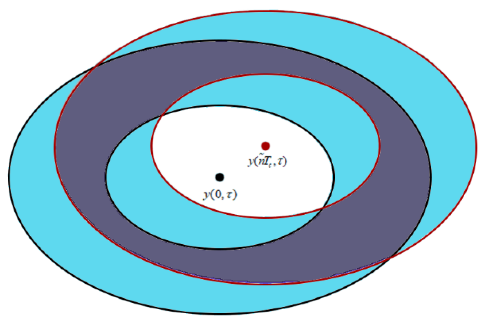
Due to the relative motion of the transmitter and the receiver, the correlation between two complex waveforms separated by $\tilde{n}{T}_c$ in time is determined by the coherence of the signals from two ocean contribution areas. These regions are elliptical, and the length of the semi-axis is related to ${\tau }_n$. The correlation between complex waveforms is defined as [19]:

$$C_y(\tilde{n}{T}_c,\tau )=\langle y(n{T}_c,\tau )y^{*}(n{T}_c+\tilde{n}{T}_c,\tau )\rangle$$

(12)

where $\tilde{n}{T}_c$ is the time interval between complex waveforms. The spatial geometry of correlation function is illustrated in Figure 3. It can be seen that the correlation between the two sea surface scattering signals gradually decreases as $\tilde{n}{T}_c$ increases. An analogous correlation between one-shot power waveforms can also be derived as:

$$C_z(\tilde{n}{T}_c,\tau )=\langle [z(n{T}_c,\tau )-\langle z(n{T}_c,\tau )\rangle ][z(n{T}_c+\tilde{n}{T}_c,\tau )-\langle z(n{T}_c+\tilde{n}{T}_c,\tau )\rangle ]\rangle$$

(13)

.

The correlation time of the signal is usually measured in milliseconds, while the time of incoherent averaging can reach the order of seconds. Thus, it can be assumed that there is no correlation between the incoherent average power waveforms, i.e., $C_Z(\tilde{t},\tau )=0$$\tilde{t}\ne 0$. The variance of the power waveform can be expressed as [21]:

$${\sigma }_Z^2(\tau )=C_Z(0,\tau )=\langle {[Z(t,\tau )-\langle Z(t,\tau )\rangle ]}^2\rangle$$

(14)

The effective incoherent average number can be reconstructed following Appendix A as [21]:

$$\frac{1}{N_{\mathrm{eff}}}=\frac{{\sigma }_Z^2(\tau )}{{\overline{Z}}^2(\tau )}=\frac{\frac{1}{N_{\mathrm{I}}}{\displaystyle \sum _{\tilde{n}=-(N_{\mathrm{I}}-1)}^{N_I-1}{\left|C_y(\tilde{n}{T}_c,\tau )\right|}^2}}{{\left|C_y(0,\tau )\right|}^2}$$

(15)

3.2. The Relationship between Model Parameters and Coherent Integration Time

As discussed in Section 3.1, the altimetric precision is determined mainly by two parameters, $S_h$ and $N_{\mathrm{eff}}$. In this section, the variables of these two parameters are derived to be expressed in terms of coherent integration time. The re-derived parameters are brought into Equation (7) to construct the coherent integration time optimization model.

3.2.1. Altimetric Sensitivity

As discussed in [28], the complex waveform is composed of useful signal and noise components

$$y(n{T}_c,\tau )=y_{\mathrm{s}}(n{T}_c,\tau )+y_{\mathrm{nd}}(n{T}_c,\tau )+y_{\mathrm{nr}}(n{T}_c,\tau )+y_{\mathrm{ndr}}(n{T}_c,\tau )$$

(16)

where $y_{\mathrm{s}}(t,\tau )$ is the cross-correlation value for the useful signal term, and $y_{\mathrm{nd}}(t,\tau )$,$y_{\mathrm{nr}}(t,\tau )$ and $y_{\mathrm{ndr}}(t,\tau )$ are the cross-correlation values of the direct and reflected noise terms.

Assuming that the signal component has no correlation with the noise components, the power waveform can be expressed as [29]:

$$Z(\tau )=\langle {\left|y_{\mathrm{s}}(n{T}_c,\tau )\right|}^2\rangle +\langle {\left|y_{\mathrm{nr}}(n{T}_c,\tau )\right|}^2\rangle +\langle {\left|y_{\mathrm{nd}}(n{T}_c,\tau )\right|}^2\rangle +\langle {\left|y_{\mathrm{ndr}}(n{T}_c,\tau )\right|}^2\rangle$$

(17)

The components above can be interpreted as the expression for the coherent integration time [18,20]:

$$\begin{array}{l}\langle {\left|y_{\mathrm{s}}(n{T}_{\mathrm{c}},\tau )\right|}^2\rangle =2P_{\mathrm{d}}{\displaystyle \iint \frac{2P_{\mathrm{t}}{G}_{\mathrm{r}}(\overrightarrow{p}){\sigma }_0}{4\pi R_{\mathrm{t}}^2(\overrightarrow{p})R_{\mathrm{r}}^2(\overrightarrow{p})}\times }{\Lambda }^2(\Delta \tau )\times {\mathrm{sinc}}^2(\Delta f{T}_{\mathrm{c}})d^{2}p\\ \langle {\left|y_{\mathrm{nr}}(n{T}_{\mathrm{c}},\tau )\right|}^2\rangle =\frac{2k{T}_{\mathrm{rec}\text{\_}\mathrm{r}}}{T_c}2P_{\mathrm{d}}\\ \langle {\left|y_{\mathrm{nd}}(n{T}_{\mathrm{c}},\tau )\right|}^2\rangle =\frac{2k{T}_{\mathrm{rec}\text{\_}\mathrm{d}}}{T_{\mathrm{c}}}2P_{\mathrm{r}}\\ \langle {\left|y_{\mathrm{ndr}}(n{T}_{\mathrm{c}},\tau )\right|}^2\rangle =\frac{2k{T}_{\mathrm{rec}\text{\_}\mathrm{r}}}{T_{\mathrm{c}}}2k{T}_{\mathrm{rec}\text{\_}\mathrm{d}}B\end{array}$$

(18)

where $B$ represents the equivalent noise bandwidth of the receiver, $T_{\mathrm{rec}\text{\_}\mathrm{d}}$ and $T_{\mathrm{rec}\text{\_}\mathrm{r}}$ represent the equivalent input noise temperature of the up-looking and down-looking chains, $P_{\mathrm{r}}$ represents the total power of the reflected signal at the input of the correlator, $P_{\mathrm{d}}$ represents the total power of the direct signal at the input of the correlator, $P_{\mathrm{t}}$ represents the power of the transmitted signal, and $G_{\mathrm{r}}$ represents the antenna gain [30,31]. Based on Equations (17) and (18), the altimetric sensitivity can be represented by the coherent integration time [5].

3.2.2. Effective Incoherent Average Number

As discussed in Equation (15), the effective incoherent average at the SP is closely related to the waveform correlation [32]. Therefore, when the processing time of the incoherent average power waveform is $T_{\mathrm{I}}$, the variation of $N_{\mathrm{eff}}$ with the coherent integration time can be approximated following Appendix B as:

$$\frac{1}{N_{\mathrm{eff}}}=\frac{T_{\mathrm{c}}{\displaystyle \sum _{\tilde{n}=-(N_{\mathrm{I}}-1)}^{N_{\mathrm{I}}-1}\left(2P_{\mathrm{d}}{\displaystyle \iint \frac{2P_{\mathrm{t}}{G}_{\mathrm{r}}(\overrightarrow{p}){\sigma }_0}{4\pi R_{\mathrm{t}}^2(\overrightarrow{p})R_{\mathrm{r}}^2(\overrightarrow{p})}{\Lambda }^2(\Delta \tau )}{\mathrm{sinc}}^2(\Delta f{T}_{\mathrm{c}}){\exp }^{-\mathrm{j}2\mathsf{\pi }\Delta f(\tilde{n}{T}_{\mathrm{c}})}{d}^{2}p+\frac{2P_{\mathrm{d}}{n}_0^{\mathrm{d}}}{T_{\mathrm{c}}}\mathrm{tri}(\frac{\tilde{n}{T}_{\mathrm{c}}}{T_{\mathrm{c}}})+\frac{B{n}_0^{\mathrm{d}}{n}_0^{\mathrm{u}}}{T_{\mathrm{c}}}\mathrm{tri}(\frac{\tilde{n}{T}_{\mathrm{c}}}{T_{\mathrm{c}}})\right)}}{T_{\mathrm{I}}\left(2P_{\mathrm{d}}{\displaystyle \iint \frac{2P_{\mathrm{t}}{G}_{\mathrm{r}}(\overrightarrow{p}){\sigma }_0}{4\pi R_{\mathrm{t}}^2(\overrightarrow{p})R_{\mathrm{r}}^2(\overrightarrow{p})}{\Lambda }^2(\Delta \tau )}{\mathrm{sinc}}^2(\Delta f{T}_{\mathrm{c}})d^{2}p+\frac{2P_{\mathrm{d}}{n}_0^{\mathrm{d}}}{T_{\mathrm{c}}}+\frac{B{n}_0^{\mathrm{d}}{n}_0^{\mathrm{u}}}{T_{\mathrm{c}}}\right)}$$

(19)

where $n_0^{\mathrm{d}}=2k{T}_{\mathrm{d}}$ and $n_0^{\mathrm{u}}=2k{T}_{\mathrm{u}}$ are the power spectral density of thermal noise from the up-looking and down-looking chains respectively, $\mathrm{tri}()$ is the triangular function, $\Delta \tau$ is the difference between ${\tau }_n$ and the scattering point delay $\tau (\overrightarrow{p})$, and $\Delta f$ is the difference between 0 Doppler and the scattering point Doppler $f(\overrightarrow{p})$.

Accordingly, the coherent integration time optimization model can be derived by simultaneously applying Equations (7) and (17)–(19). In accordance with Equation (17), a larger coherent integration time is needed to improve the altimetric sensitivity and precision. Nevertheless, the limitation of $N_{\mathrm{eff}}$ on the altimetric precision leads to a relatively smaller expected value of the coherent integration time. As a consequence, the best precision result is achieved by balancing the time required for the coherent integration of both aspects.

4. Results and Application

4.1. Validation of Coherent Integration Time Optimization Model

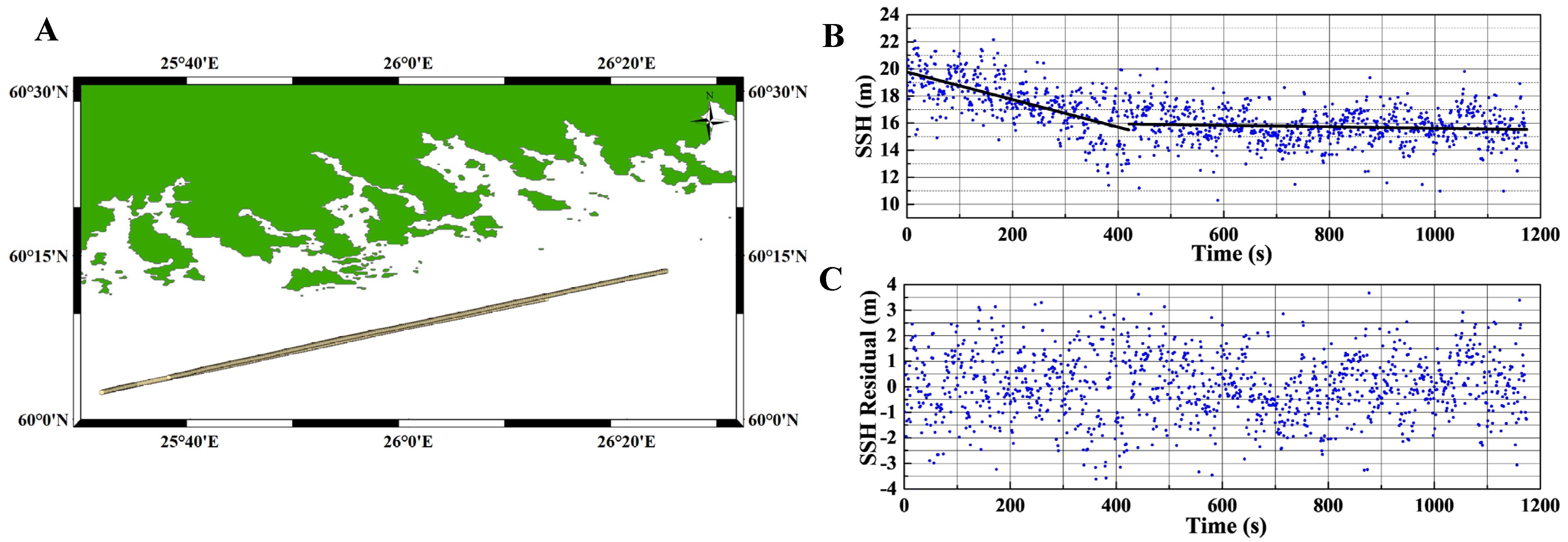
The proposed model precision results are compared with the experimental results to verify the effectiveness of the coherent integration time optimization model in this section. The measured precision is calculated as described in Section 2. With the power waveform processing time $T_{\mathrm{I}}=1 \mathrm{s}$ unchanged, the precision variation ${\sigma }_h^{\mathrm{obs}}(T_c)$ with coherent integration time can be determined by varying the value of $T_c$. To avoid the error interference caused by aircraft turning, two straight flight trajectories are selected for precision calculations. Figure 4B illustrates the inverted SSH sequence when $T_c$ is 10 ms during the experiment. The corresponding SSH residual sequence is shown in Figure 4C.

The coherent integration time optimization model has been acquired in the following steps as described in Section 3. Obtain auxiliary data during the experiment, including the position and velocity information of the receiver after dual-frequency orbit determination, the GPS satellite position and velocity using the IGS precision ephemeris interpolation method, wind speed (~7 m/s) and payload parameters. These simulation parameters are listed in

Table 1. Air-based simulation parameters that are consistent with those for the experiment described in Section 2.

Design Parameter	Value
Receiver height	~3000 m
Transmitter altitude	20,200 km
Receiver velocity	50 m/s
Antenna temperature	200 K
Antenna gain	15 dBi
Elevation angle	70°
Processing interval	39,102–40,721
Power waveform processing time	1 s
Wind speed	7 m/s
Process method	iGNSS-R
Sampling frequency	80 MHz
Carrier frequency	1575.42 MHz (GPS L1)
Receiver bandwidth	35 MHz
Waveform retracking method	DER
Filter bandwidth	12 MHz

. The elevation angle is computed with the bistatic geometry. The computation of the variations in the effective incoherent average number and altimeric sensitivity with coherent integration time can be obtained by applying Equations (17)–(19). By substituting the intermediate results into Equation (7), the coherent integration time optimization model can be calculated.

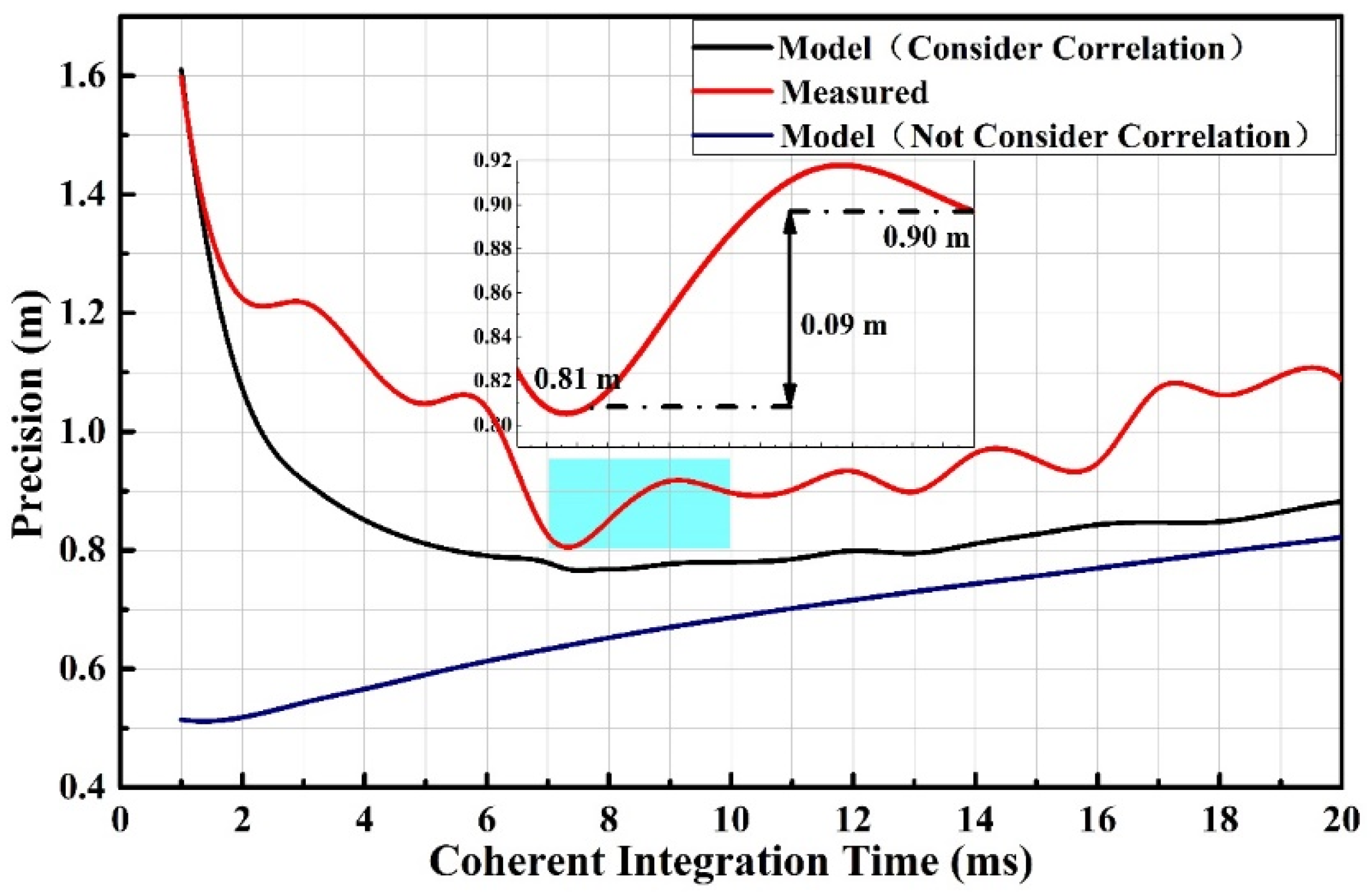
A comparison between the variance of the model and the measured result is shown in Figure 5. To evaluate the effectiveness of the model, the mean deviation of precision $\langle \left|{\sigma }_h^{\mathrm{m}}(T_c)-{\sigma }_h^{\mathrm{obs}}(T_c)\right|\rangle$ is used. ${\sigma }_h^{\mathrm{m}}(T_c)$ is the precision calculated by the model, whereas ${\sigma }_h^{\mathrm{obs}}(T_c)$ is the measured precision. The results show that the average deviation between the red and blue curves is 0.85 m, and the average deviation between the red and black curves is 0.16 m. Therefore, the proposed model considering the correlation of the waveforms is in good agreement with the measured result.

The model curve and the measured curve differ by a certain amount. On the one hand, the measured precision result is generally worse than that of the model, with an average of 0.16 m. This may be due to the lack of beamforming in the signal processing, which causes the SNR to decrease. On the other hand, the trend of the measured curve fluctuates. As opposed to the simulated results, the actual measurement results may contain other stochastic factors such as aircraft mechanical vibrations, attitude changes, and antenna pointing, etc. These random factors can be used to optimize the model by obtaining recorded data of aircraft attitude and vibration in the future.

4.1.1. Altimetric Sensitivity

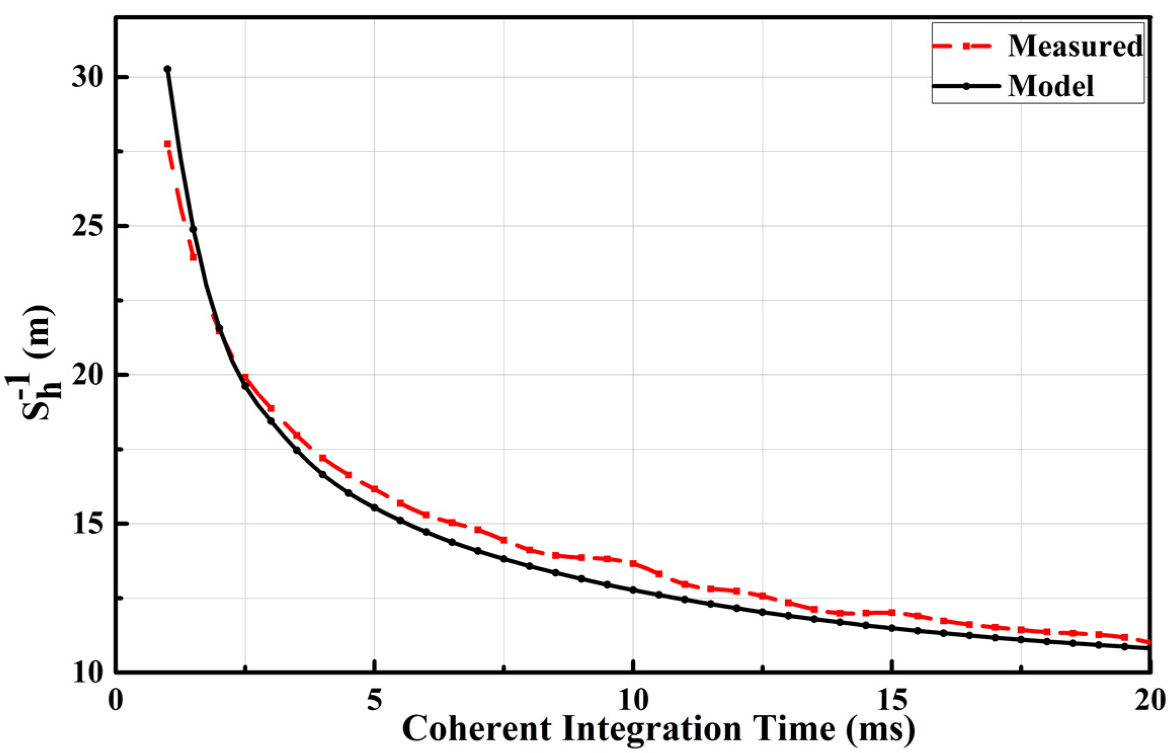
The reciprocal of the altimetric sensitivity simulation is compared with the measured result, as shown in Figure 6. It can be appreciated that the measured and the simulated curves are in good agreement. As the coherent integration time increases, the reciprocal of the sensitivity approaches a limit value. The difference between the curves may be caused by unaccounted noises [33,34].

4.1.2. Effective Incoherent Average Number

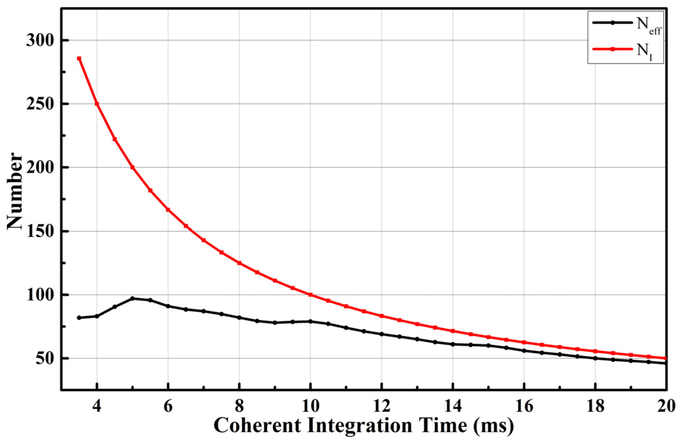
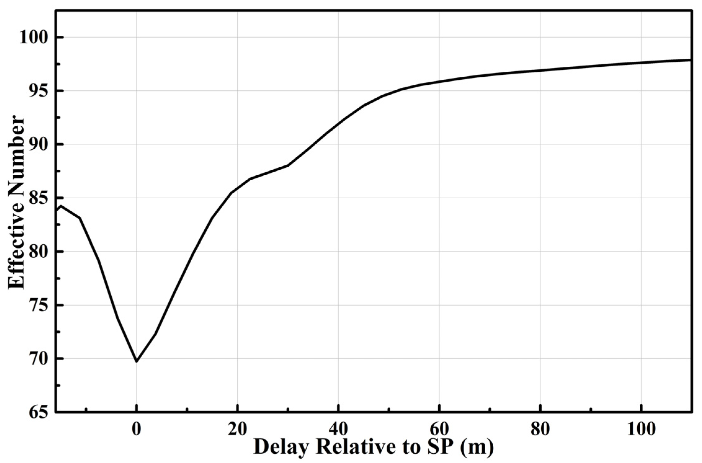
It can be seen from Equation (19) that the effective incoherent average is a nonlinear function of the coherent integration time. The variations of $N_{\mathrm{I}}$ and $N_{\mathrm{eff}}$ with the coherent integration time are compared, as shown in Figure 7. It reveals that when $T_{\mathrm{I}}$ is constant, $N_{\mathrm{I}}$ and $T_c$ are inversely proportional. However, $N_{\mathrm{eff}}$ and $T_c$ are non-linearly related. The difference between $N_{\mathrm{eff}}$ and $N_{\mathrm{I}}$ will gradually decrease as the coherent integration time increases. If there were no correlation between the waveforms i.e., $C_y(\tilde{n}{T}_c,\tau )=0,\tilde{n}\ne 0$, then $N_{\mathrm{eff}}$ would be equal to $N_{\mathrm{I}}$. $N_{\mathrm{eff}}$ also varies with the length delay $c{\tau }_n$ as shown in Figure 8. It is a hybrid effect of SNR and Doppler bandwidth at different delays [35].

4.2. Application of Coherent Integration Time Optimization Model

The conformity between the model and the measured results indicates that the proposed model can better reflect the influence of coherent integration time on the altimetric precision. Consequently, the model can be used to determine the optimal coherent integration time to improve experimental data processing. In addition, the model can be applied to a variety of altimetry situations to provide a theoretical reference for data optimization processing.

4.2.1. Model Application: Airborne Experiment Scenario

In the airborne altimetry scene described in Section 4.1, the traditional integration parameters cannot yield the optimal precision. In constructing a coherent integration time optimization model based on the same experimental parameters, the optimal coherent integration time is calculated to be 7.5 ms, as shown in Figure 5. By applying this integral parameter to the processing of the measured data, the precision is 0.81 m. As compared to the empirical coherent integration (10 ms) [21], the altimetric precision is improved by 0.09 m.

4.2.2. Model Application: Extrapolation to Spaceborne Scenario

Given the reasonable levels of agreement between the simulated model and the airborne experimental data, the proposed coherent integration time optimization model has been implemented to simulate spaceborne iGNSS-R data. Since there is no dedicated iGNSS-R altimetry satellite at present, the results of model optimization can provide a theoretical reference for improving the in-orbit performance of an iGNSS-R-based ocean altimeter in the future. The altimetric precision is mainly determined by the system instrument parameters and observation geometry. These factors will lead to different model optimization results. According to the model’s expression, the main parameters that affect the precision are respectively analyzed, including the receiver’s orbital altitude, sea surface roughness, elevation angle, and antenna gain. Previously, these parameters were discussed, and this section re-evaluates them in light of the novel model [31,36]. It needs to be clarified that the Z-V model does not account for the influence of coherent scattering under low wind speed conditions; the minimum wind speed is set to 4 m/s to avoid errors caused by the simulation waveform. The fixed system parameters are summarized in

Table 2. The common simulation parameters for spaceborne altimetry scenarios.

Design Parameter	Value
Receiver bandwidth	35 MHz
Antenna temperature	200 K
Transmitter altitude	20,200 km
Process method	iGNSS-R
Sampling rate	80 MHz
Carrier frequency	1575.42 MHz (GPS L1)
Waveform retracking method	DER
Filter bandwidth	12 MHz
Power waveform processing time	1 s

. The dependence of the precision variation and the optimal coherent integration time on different parameters is analyzed as follows.

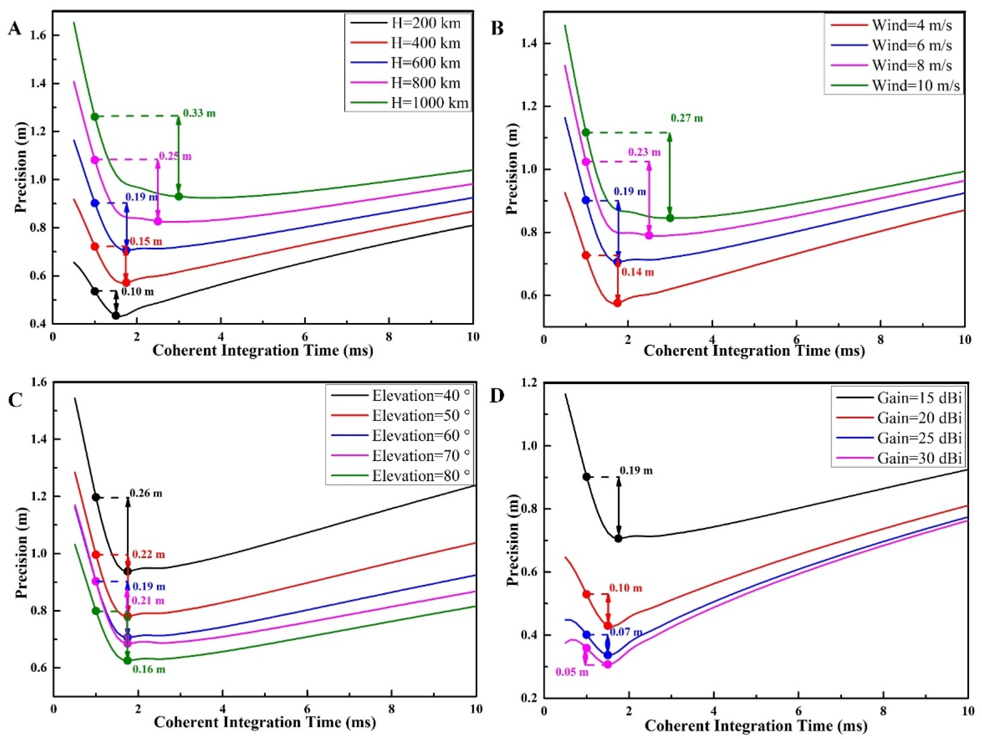
As can be seen from Figure 9:

(1) As shown in Figure 9A, the precision decreases with the altitude of the orbit. When the orbit altitude increases from 200 km to 1000 km, the optimal precision decreases from 0.43 m to 0.94 m. This is because, according to Equation (17), the signal power decreases squarely with the transmission distance, causing the SNR to decrease. On the other hand, the receiver velocity decreases with altitude, resulting in increased waveform correlation and decreased effective incoherent average.

As the orbital altitude increases, the optimal coherent integration time increases from 1.5 ms to 3 ms. Higher altitude results in greater energy loss, which calls for a longer time for coherent integration, which improves the SNR and therefore the altimetric sensitivity. The higher the orbital altitude of the receiver, the more noticeable the improvement in precision of the optimal coherent integration time when compared to the empirical spaceborne coherent integration parameters (1 ms). Therefore, the coherent integration time optimization model is preferred for improving the altimetric precision under the low SNR conditions.

(2) As shown in Figure 9B, the precision decreases with wind speed. With an increase in wind speed from 4 m/s to 10 m/s, the optimal precision decreases from 0.57 m to 0.85 m. At low wind speeds, the sea surface is smooth, the waveform coherence is strong, and the effective incoherent average is small. However, the SNR is high, which enhances precision.

The optimal coherent integration time will increase from 1.6 ms to 3 ms with wind speed. This is because high wind speed increases ocean scattering. Simultaneously, the higher the wind speed, the worse the SNR, and the greater the precision improved by the optimal coherent integration time.

(3) In Figure 9C, the optimal precision increases from 0.94 m to 0.63 m as the elevation angle changes from 40° to 80°. On the one hand, increasing the elevation angle shortens the propagation path of the navigation signal, which reduces the signal energy loss. On the other hand, according to Figure 3, the iso-delay area decreases with the elevation angle, thereby increasing the effective incoherent average.

Since both the altimetric sensitivity and the effective incoherent average decrease with the elevation angle, the balance between the two leads to little change in the optimal coherent integration time. Accordingly, as the elevation angle increases, the SNR of the reflected signal upgrades and the improvement of the precision by the optimal coherent integration time becomes insignificant.

(4) As illustrated in Figure 9D, when the antenna gain is increased from 15 dBi to 30 dBi, the optimal precision improves from 0.72 m to 0.31 m. The high gain antenna can increase signal energy and upgrade the SNR. When the antenna gain is increased from 25 dBi to 30 dBi, the optimal precision is only improved from 0.34 m to 0.31 m. This indicates that an increase in antenna gain will not be sufficient to improve precision at high SNRs.

Similarly, the optimal coherent integration time does not greatly improve the precision in the case of high gain. Since the change of the antenna gain does not affect the effective incoherent average, the optimal coherent integration time does not change much with the antenna gain.

(5) In general, the optimal coherent integration time calculated in the spaceborne simulation is shorter than that for the airborne scenario. This is because the satellite receiver has a high velocity, making the Doppler bandwidth and the effective incoherent average large. The shorter coherent integration time can effectively reduce the influence of speckle noise.

The simulation analysis of the above parameters indicates that the coherent integration time optimization model improves the precision more significantly when the SNR of the reflected waveform is relatively weak. Limited by the code bandwidth, improving the SNR of the signal does not increase the precision infinitely but approaches the limit value. Additionally, the optimal coherent integration time varies with the simulation parameters, and the spaceborne scenario tends to be shorter than the airborne scenario. Increasing the altitude of the orbit and the wind speed will also increase the optimal coherent integration time.

5. Conclusions

This paper constructs a coherent integration time optimization model from the perspective of signal processing to improve iGNSS-R ocean altimetric precision. The research mainly involves three aspects: the processing of IF data and the extraction of precision information; the derivation and verification of the coherent integration time optimization model; and the application of the validated model to airborne and spaceborne altimetry mission scenarios to predict the optimal solution for precision.

(1) To estimate the SP delay for airborne data processing, we use the DER method. The altimetric precision is evaluated based on the random characteristics of the SSH. (2) For the purpose of optimizing the precision performance, we consider the influence of the correlation between waveforms on the covariance of the power waveform, and derive the coherent integration time optimization model from the statistical properties of the waveform. The model is verified by airborne measurements. Results indicate that the average deviation between model and measurement precisions is 0.16 m, which is acceptable. (3) Based on the optimal coherent integration time of the model solution, we processed the experimental data, and the precision is improved by about 0.1 m relative to that obtained using the empirical parameters. The positive validation of the coherent integration time optimization model provides a tool for evaluating the optimal coherent integration time and its precision under different orbital altitudes, sea surface roughness, elevation angles, and antenna gains in spaceborne iGNSS-R altimetry scenarios. The results show that the optimal coherent integration time for the spaceborne scene is shorter than that for the airborne scene. In the case of low SNR, the model can improve the precision to the decimeter level. Due to the combined effect of the SNR and the Doppler bandwidth, the optimal coherent integration time increases with the orbit altitude and the sea surface roughness.

The coherent integration time optimization model developed in this paper is capable of optimizing the waveform processing parameters and improving the altimetric precision. It can be applied to the optimization of data processing and high-precision retrieval for future spaceborne iGNSS-R altimetry missions. In future research, we will also analyze and evaluate the influence of the calibration errors of the instrument, the receiver orbit, and the atmosphere on the precision.

References

- Martin-Neira, M. A Passive Reflectometry and Interferometry System (PARIS): Application to ocean altimetry. ESA J. 1993, 17, 331–355. [Google Scholar]
- Lowe, S.T.; Zuffada, C.; LaBrecque, J.L.; Lough, M.; Lerma, J.; Young, L.E. An ocean-altimetry measurement using reflected GPS signals observed from a low-altitude aircraft. IEEE Int. Geosci. Remote Sens. Symp. 2000, 5, 2185–2187. [Google Scholar] [CrossRef]
- Beyerle, G.; Hocke, K. Observation and simulation of direct and reflected GPS signals in radio occultation experiments. Geophys. Res. Lett. 2001, 28, 1895–1898. [Google Scholar] [CrossRef]
- Foti, G.; Gommenginger, C.; Jales, P.; Unwin, M.; Shaw, A.; Robertson, C.; Rosello, J. Spaceborne GNSS reflectometry for ocean winds: First results from the UK TechDemoSat-1 mission. Geophys. Res. Lett. 2015, 42, 5435–5441. [Google Scholar] [CrossRef] [Green Version]
- Martin-Neira, M.; Caparrini, M.; Font-Rossello, J.; Lannelongue, S.; Vallmitjana, C.S. The PARIS concept: An experimental demonstration of sea surface altimetry using GPS reflected signals. IEEE Trans. Geosci. Remote Sens. 2001, 39, 142–150. [Google Scholar] [CrossRef] [Green Version]
- Carreno-Luengo, H.; Camps, A.; Ramos-Perez, I.; Rius, A. Experimental evaluation of GNSS reflectometry altimetric precision using the P(Y) and C/A signals. IEEE J. Sel. Top. Appl. Earth Obs. Remote Sens. 2014, 7, 1493–1500. [Google Scholar] [CrossRef]
- Li, W.; Yang, D.; D’Addio, S.; Martin-Neira, M. Partial interferometric processing of reflected GNSS signals for ocean altimetry. Geophys. Res. Lett. 2014, 11, 1509–1513. [Google Scholar] [CrossRef]
- Cardellach, E.; Rius, A.; Martin-Neira, M.; Fabra, F.; Nogues-Correig, O.; Ribo, S.; Kainulainen, J.; Camps, A.; D’Addio, S. Consolidating the precision of interferometric GNSS-R ocean altimetry using airborne experimental data. IEEE Trans. Geosci. Remote Sens. 2014, 52, 4992–5004. [Google Scholar] [CrossRef]
- Feng, W.; Yang, D.; Li, W.; Wei, Y. On-ground retracking to correct distorted waveform in spaceborne global navigation satellite system-reflectometry. Remote Sens. 2017, 9, 643. [Google Scholar] [CrossRef] [Green Version]
- Hajj, G.A. Theoretical description of a bistatic system for ocean altimetry using the GPS signa. Radio Sci. 2003, 38, 1001–1019. [Google Scholar] [CrossRef]
- Fernando Marchan-Hernandez, J.; Camps, A.; Rodriguez-Alvarez, N.; Valencia, E.; Bosch-Lluis, X.; Ramos-Perez, I. An efficient algorithm to the simulation of delay-Doppler maps of reflected global navigation satellite system signals. IEEE Trans. Geosci. Remote Sens. 2009, 47, 2733–2740. [Google Scholar] [CrossRef]
- Rius, A.; Cardellach, E.; Martin-Neira, M. Altimetric analysis of the sea-surface GPS-reflected signals. IEEE Trans. Geosci. Remote Sens. 2010, 48, 2119–2127. [Google Scholar] [CrossRef]
- Rodríguez, E. Altimetry for non-Gaussian oceans: Height biases and estimation of parameters. J. Geophys. Res. 1988, 93, 14107–14120. [Google Scholar] [CrossRef]
- Mashburn, J.; Axelrad, P.; Lowe, S.T.; Larson, K.M. Global ocean altimetry with GNSS reflections from TechDemoSat-1. IEEE Trans. Geosci. Remote Sens. 2018, 56, 4088–4097. [Google Scholar] [CrossRef]
- Li, W.; Cardellach, E.; Fabra, F.; Ribo, S.; Rius, A. Assessment of spaceborne GNSS-R ocean altimetry performance using CYGNSS mission raw data. IEEE Trans. Geosci. Remote Sens. 2019, 58, 238–250. [Google Scholar] [CrossRef]
- Liu, Z.; Zheng, W.; Wu, F.; Cui, Z.; Kang, G. A necessary model to quantify the scanning loss effect in spaceborne iGNSS-R ocean altimetry. IEEE J. Sel. Top. Appl. Earth Obs. Remote Sens. 2021, 14, 1619–1627. [Google Scholar] [CrossRef]
- Liu, Z.; Zheng, W.; Wu, F.; Kang, G.; Li, Z.; Wang, Q.; Cui, Z. Increasing the number of sea surface reflected signals received by GNSS-Reflectometry altimetry satellite using the nadir antenna observation capability optimization method. Remote Sens. 2019, 11, 2473. [Google Scholar] [CrossRef] [Green Version]
- Martin-Neira, M.; D’Addio, S.; Buck, C.; Floury, N.; Prieto-Cerdeira, R. The PARIS ocean altimeter in-orbit demonstrator. IEEE Trans. Geosci. Remote Sens. 2011, 49, 2209–2237. [Google Scholar] [CrossRef]
- You, H.I.; Garrison, J.L.; Heckler, G.; Zavorotny, V.U. Stochastic voltage model and experimental measurement of ocean-scattered GPS signal statistics. IEEE Trans. Geosci. Remote Sens. 2004, 42, 2160–2169. [Google Scholar] [CrossRef]
- Garrison, J.L. A statistical model and simulator for ocean-reflected GNSS signals. IEEE Trans. Geosci. Remote Sens. 2016, 54, 6007–6019. [Google Scholar] [CrossRef]
- Li, W.; Rius, A.; Fabra, F.; Cardellach, E.; Ribo, S.; Martin-Neira, M. Revisiting the GNSS-R waveform statistics and its impact on altimetric retrievals. IEEE Trans. Geosci. Remote Sens. 2018, 56, 2854–2871. [Google Scholar] [CrossRef]
- Jing, C.; Niu, X.; Duan, C.; Lu, F.; Di, G.; Yang, X. Sea surface wind speed retrieval from the first Chinese GNSS-R mission: Technique and preliminary results. Remote Sens. 2019, 11, 3013. [Google Scholar] [CrossRef] [Green Version]
- Fabra, F.; Cardellach, E.; Ribo, S.; Li, W.; Rius, A.; Carlos Arco-Fernandez, J.; Nogués-Correig, O.; Praks, J.; Rouhe, E.; Seppänen, J.; et al. Is accurate synoptic altimetry achievable by means of interferometric GNSS-R? Remote Sens. 2019, 11, 505. [Google Scholar] [CrossRef] [Green Version]
- Ribo, S.; Arco-Fernandez, J.C.; Cardellach, E.; Fabra, F.; Li, W.; Nogues-Correig, O.; Rius, A.; Martín-Neira, M. A software-defined GNSS reflectometry recording receiver with wide-bandwidth, multi-band capability and digital beam-forming. Remote Sens. 2017, 9, 450. [Google Scholar] [CrossRef] [Green Version]
- Park, H.; Camps, A.; Valencia, E.; Rodriguez-Alvarez, N.; Bosch-Lluis, X.; Ramos-Perez, I.; Carreno-Luengo, H. Retracking considerations in spaceborne GNSS-R altimetry. GPS Solut. 2012, 16, 507–518. [Google Scholar] [CrossRef]
- Zavorotny, V.U.; Voronovich, A.G. Scattering of GPS signals from the ocean with wind remote sensing application. IEEE Trans. Geosci. Remote Sens. 2000, 38, 951–964. [Google Scholar] [CrossRef] [Green Version]
- Mashburn, J.; Axelrad, P.; Lowe, S.T.; Larson, K.M. An assessment of the precision and accuracy of altimetry retrievals for a monterey bay GNSS-R experiment. IEEE J. Sel. Top. Appl. Earth Observ. Remote Sens. 2016, 9, 4660–4668. [Google Scholar] [CrossRef]
- D’Addio, S.; Martin-Neira, M.; di Bisceglie, M.; Galdi, C.; Martin Alemany, F. GNSS-R altimeter based on Doppler multi-looking. IEEE J. Sel. Top. Appl. Earth Obs. Remote Sens. 2014, 7, 1452–1460. [Google Scholar] [CrossRef]
- D’Addio, S.; Martin-Neira, M. Comparison of processing techniques for remote sensing of earth-exploiting reflected radio-navigation signals. Electron. Lett. 2013, 49, 292–293. [Google Scholar] [CrossRef]
- Fan, M.; Zhang, B.; Wang, F. Semi-codeless based P(Y) code autocorrelation GNSS-R sea surface altimetry method. J. Beijing Univ. Aeronaut. Astronaut. 2019, 45, 398–404. [Google Scholar] [CrossRef]
- Martin, F.; Camps, A.; Park, H.; D’Addio, S.; Martin-Neira, M.; Pascual, D. Cross-correlation waveform analysis for conventional and interferometric GNSS-R approaches. IEEE J. Sel. Top. Appl. Earth Obs. Remote Sens. 2014, 7, 1560–1572. [Google Scholar] [CrossRef]
- Camps, A.; Park, H.; Domènech, E.V.; Pascual, D.; Martin, F.; Rius, A.; Ribo, S.; Benito, J.; Andrés-Beivide, A.; Saameno, P.; et al. Optimization and performance analysis of interferometric GNSS-R altimeters: Application to the Paris IoD mission. IEEE J. Sel. Top. Appl. Earth Obs. Remote Sens. 2014, 7, 1436–1451. [Google Scholar] [CrossRef]
- Wu, F.; Zheng, W.; Li, Z.; Liu, Z. Improving the GNSS-R specular reflection point positioning accuracy using the gravity field normal projection reflection reference surface combination correction method. Remote Sens. 2018, 11, 33. [Google Scholar] [CrossRef] [Green Version]
- Wu, F.; Zheng, W.; Li, Z.; Liu, Z. Improving the positioning accuracy of satellite-borne GNSS-R specular reflection point on sea surface based on the ocean tidal correction positioning method. Remote Sens. 2019, 11, 1626. [Google Scholar] [CrossRef] [Green Version]
- Zavorotny, V.U.; Gleason, S.; Cardellach, E.; Camps, A. Tutorial on remote sensing using GNSS bistatic radar of opportunity. IEEE Geosci. Remote Sens. Mag. 2014, 2, 8–45. [Google Scholar] [CrossRef] [Green Version]
- Carreno-Luengo, H.; Park, H.; Camps, A.; Fabra, F.; Rius, A. GNSS-R Derived Centimetric Sea Topography: An Airborne Experiment Demonstration. IEEE J. Sel. Top. Appl. Earth Observ. Remote Sens. 2013, 6, 1468–1478. [Google Scholar] [CrossRef]
- Goodman, J.W.; Narducci, L.M. Statistical Optics. Phys. Today 1986, 39, 126. [Google Scholar] [CrossRef]
Figure 1.
Simplified flowchart of airborne IF data processing.
Figure 2.
Examples of measured and simulated power waveforms. (A) Normalized measured power waveform processed from the IF data. The is the maximum point of the first derivative. (B) Normalized simulated power waveform generated based on the Z-V model. The is the maximum point of the first derivative. The is the nominal SP calculated based on the WGS-84 reference ellipsoid.
Figure 3.
Sea surface contribution area corresponding to .
Figure 4.
Experimental area and IF data processing results. (A) The specular points tracks of the raw IF data. (B) Measured SSH relative to the WGS84 reference ellipsoid. (C) SSH residual after subtracting the fitted value.
Figure 5.
The variation of the precision with coherent integration time under different conditions. Red indicates the measured result. Black indicates the model result considering the correlation between the waveforms. Blue indicates the model result without considering the correlation between the waveforms.
Figure 6.
A comparison of the reciprocal value of altimetric sensitivity between measured (red) and simulated data (black).
Figure 7.
Comparison of the effective incoherent average number (black) and the incoherent average number (red).
Figure 8.
Effective incoherent average number relative to SP.
Figure 9.
The simulation variation curves of the estimated altimetric precision with the coherent integration time under different conditions. (A) When the wind speed is 6 m/s, the elevation is 60°, the antenna gain is 15 dBi, and the orbit altitude varies. (B) When the orbit altitude is 600 km, the elevation is 60°, the antenna gain is 15 dBi, and the wind speed varies. (C) When the orbit altitude is 600 km, the wind speed is 6 m/s, the antenna gain is 15 dBi, and the elevation varies. (D) When the orbit altitude is 600 km, the wind speed is 6 m/s, the elevation is 60°, and the antenna gain varies.