Quick Detection of Field-Scale Soil Comprehensive Attributes via the Integration of UAV and Sentinel-2B Remote Sensing Data

Abstract

Satellite and unmanned aerial vehicle (UAV) remote sensing can be used to estimate soil properties; however, little is known regarding the effects of UAV and satellite remote sensing data integration on the estimation of soil comprehensive attributes, or how to estimate quickly and robustly. In this study, we tackled those gaps by employing UAV multispectral and Sentinel-2B data to estimate soil salinity and chemical properties over a large agricultural farm (400 ha) covered by different crops and harvest areas at the coastal saline-alkali land of the Yellow River Delta of China in 2019. Spatial information of soil salinity, organic matter, available/total nitrogen content, and pH at 0–10 cm and 10–20 cm layers were obtained via ground sampling (n = 195) and two-dimensional spatial interpolation, aiming to overlap the soil information with remote sensing information. The exploratory factor analysis was conducted to generate latent variables, which represented the salinity and chemical characteristics of the soil. A machine learning algorithm (random forest) was applied to estimate soil attributes. Our results indicated that the integration of UAV texture and Sentinel-2B spectral data as random forest model inputs improved the accuracy of latent soil variable estimation. The remote sensing-based information from cropland (crop-based) had a higher accuracy compared to estimations performed on bare soil (soil-based). Therefore, the crop-based approach, along with the integration of UAV texture and Sentinel-2B data, is recommended for the quick assessment of soil comprehensive attributes.

1. Introduction

Optimizing agricultural management practices, such as efficient and sustainable irrigation and fertilization, are effective ways to improve soil quality across vast coastal saline-alkali regions [1,2,3]. Among fertilization, organic and nitrogen fertilizers are commonly used to enhance soil quality. The organic fertilizers/amendments have notable capabilities in improving soil structure and water holding capacity since the organic carbon from amendments works as a bonder to bind silt and clay particles together for the micro-aggregate formation [4,5]. However, the salinity adversely impacts the soil organic carbon content [6,7]. The absorption of potassium, phosphorus, and other necessary elements from crops is reduced by the Sodium (Na⁺) competition [8]. Appropriate nitrogen fertilizer improves the leaf area extension, leaf life prolongment, and increasing of the chlorophyll content, thus facilitating the photosynthetic process of vegetation and increasing biomass accumulation [9]. Generally, nitrogen acts as a limiting nutrient factor in coastal regions [10], because a high salt content usually causes a large volume of $N{O}_3^{-}$-N concentration leachate [11], restricting the nitrification process and root uptake, and increasing NH₃ volatilization [12]. Nevertheless, excessive nitrogen application accelerates environmental pollution and soil salinization through the release of a higher quantity of base cations to soil solution [1]. Under such circumstances, it is fundamental to diagnose the spatial variance of soil properties across saline-alkali soils. Besides, in the field of modern precision agriculture, quick assessment of comprehensive soil attributes is important for agronomic management over a large farm, thus, the development of latent soil variables that consider both the fertility and salinity levels of soil is key to achieving this goal [13].

Traditional ground investigations of soil quality are time and labor-intensive in large-scale impact assessments, while currently, remote sensing imagery and derivative products are feasible in providing rapid non-destructive estimations [14,15]. Satellite remote sensing is characterized by the large-area coverage, while the airborne system such as the unmanned aerial vehicle (UAV) has advantages of flexibility and high spatial resolutions. In recent years, the integration of UAV and satellite remote sensing has been applied to the detection/estimation of soil attributes [16,17]. Generally, these studies often calibrated soil attribute estimation models by developing the regression relationships between the soil attributes and UAV remote sensing indicators and then applying these UAV-based calibrated models to the satellite data to improve estimation accuracy at a large extension [18]. It should be noted that remote sensing-based regression models are sensor dependent since different sensors have distinct spectral channels, thus leading to distinctive information [19]. The UAV-based calibration of models could yield uncertainties when they are transferred to satellite-based applications [18]; therefore, it is important to find an alternative to integrate UAV and satellite imageries for soil attribute detection.

Remotely sensed information can be divided into several types according to their different detection approaches and spectral channels—e.g., optical, thermal, and microwave remote sensing [20,21]. Among these approaches, optical remote sensing has been widely applied in the detection of soil salinity and fertility [22], owing to its abundant information. In the field of optical remote sensing, analyzing the soil reflectance is a direct way to investigate soil features, and this soil-based approach is often based on hyperspectral remote sensing, focusing more on the selection of sensitive bands for soil attributes detection. For instance, Weng et al. (2010) applied a spectral index derived from the EO-1 Hyperion data to identify sensitive bands for the estimation of soil salinity in the Yellow River Delta [23]. More studies tended to investigate the relationships between vegetation reflectance and soil properties—an indirect means for soil quality mapping (denoted as crop-based approach), because most of the land surface is covered by vegetation instead of bare soil, and vegetation growth and development is remarkably impacted by soil properties [24,25]. For instance, the nitrogen deficiency resulted in acceleration of the leaf senescence and a reduced photosynthesis rate [26]. The study of Zhu et al. (2021) analyzed the ground-based hyperspectral reflectance of winter wheat to identify the crop growth discrepancy caused by the different soil salinity levels across soil layers [27]; the study of Song et al. (2016) integrated the Landsat thematic, spectral, and terrain images with digital elevation models to map soil salinity and evaluated the influence of vegetation on soil salinity estimation [28]. However, previous studies did not compare the performance of the soil-based and crop-based approaches in capturing soil fertility and salinity estimation.

The studies that integrated UAV and satellite remote sensing for soil quality detection mainly used spectral/vegetation indices (VIs) that are calculated using band reflectance following certain mathematical rules [29,30]. However, texture information should be highlighted as another promising advantage of UAV data, which is an informative indicator of the architecture of objects and has therefore been applied in crop growth monitoring with satisfying accuracy [31]. On the other side, commonly used UAV multispectral sensors usually have 3–6 bands, less than some satellite sensors such as Sentinel-2 (13 bands). To merge the advantages of high spatial resolution of UAV images and abundant spectral information of satellite images, the integration of UAV texture and satellite spectral information for soil fertility and salinity estimation should be investigated whilst this issue remains to be elucidated.

This study aimed to find an effective and quick approach to map and monitor the soil fertility and salinity using UAV multispectral and Sentinel-2B satellite remote sensing data. Research questions are: (1) whether the estimation accuracy of soil latent variables using crop remote sensing data is a better representative of soil attributes compared to estimations performed on the bare soil; and (2) if the integration of Sentinel-2 spectral and UAV texture variables improves the accuracy of the soil latent variable estimation.

2. Materials and Methods

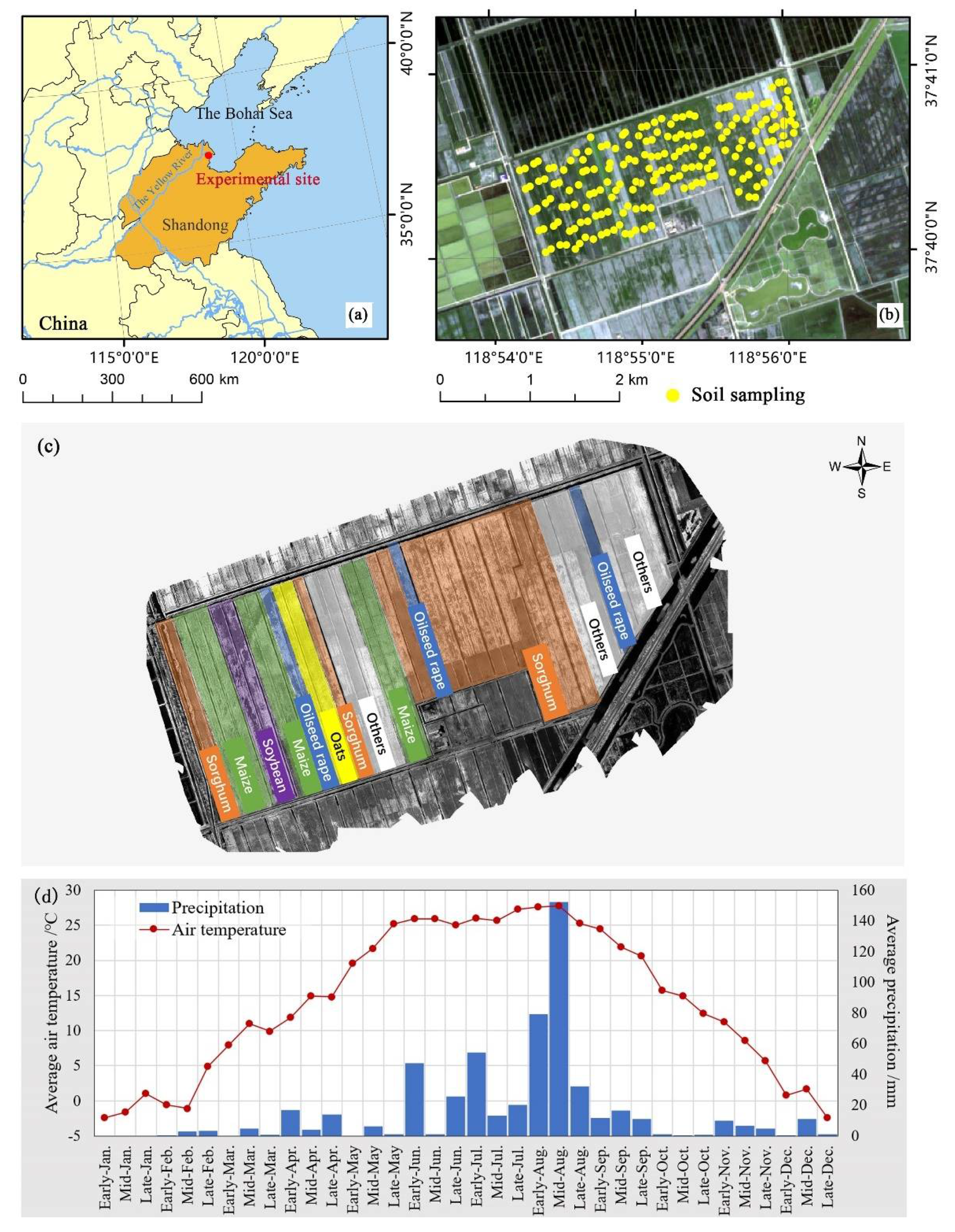
2.1. Description of the Study Area and Experimental Sites

The study area (118.90–118.93° E, 37.67–37.68° N) is located at the Yellow River Delta Research Centre of the Institute of Geographical Sciences and Natural Resources Research, Chinese Academy of Sciences, south of the Yellow River and close to the Bohai Sea (~10 km) (Figure 1), and is characterized by a temperate monsoon climate with an average annual air temperature of 12.5 °C and rainfall of 555.9 mm. Concentrated precipitation falls in summer, accounting for 65.6% of the annual precipitation, and 3.7% of precipitation is in winter. During the growing season of maize and sorghum (May–September) in 2019, the average air temperature was 24.7 °C, and the total precipitation was 472.6 mm, accounting for 85.1% of the annual total precipitation (Figure 1d). The terrain is flat, and this region was formed by the sediment of the Yellow River and is developing rapidly. Since the Yellow River Delta (YRD) suffers the seawater encroachment and relative high evapotranspiration of temperate monsoon climate, this region has a high proportion of coastal saline-alkali land (~50%) [32,33,34], which adversely impacts the cropland use efficiency of the region [35,36].

The area of the experimental site is about 400 ha, and the length and width of each strip plot are around 1.2 km and 50 m, respectively. Ditches are distributed between each plot for irrigation and flood discharge. The Yellow River water was used for irrigation. This experimental site is a typical coastal saline-alkaline land, which was reclaimed in 2017. The soil salinity level is severe and exhibits remarkable variations, and, consequently, significant vegetation variations in space. Severe salinity, along with leaching due to heavy rainfalls and irrigation, limits crop access to nitrogen, so nitrogen acted as the most critical yield-limiting nutrient for the study region. Several crops are cultivated at the experimental site, including maize (Zea mays L.), sorghum (Sorghum bicolor (L.) Moench), soybeans (Glycine max (Linn.) Merr.), oats (Avena sativa L.), and oilseed rape (Brassica napus L.). Maize and sorghum were selected as study crops based on the planting area size to compare with bare soil. The sowing dates of maize and sorghum were 17 May and 22 May in 2019, respectively. The agronomic management was uniform throughout the whole experimental site.

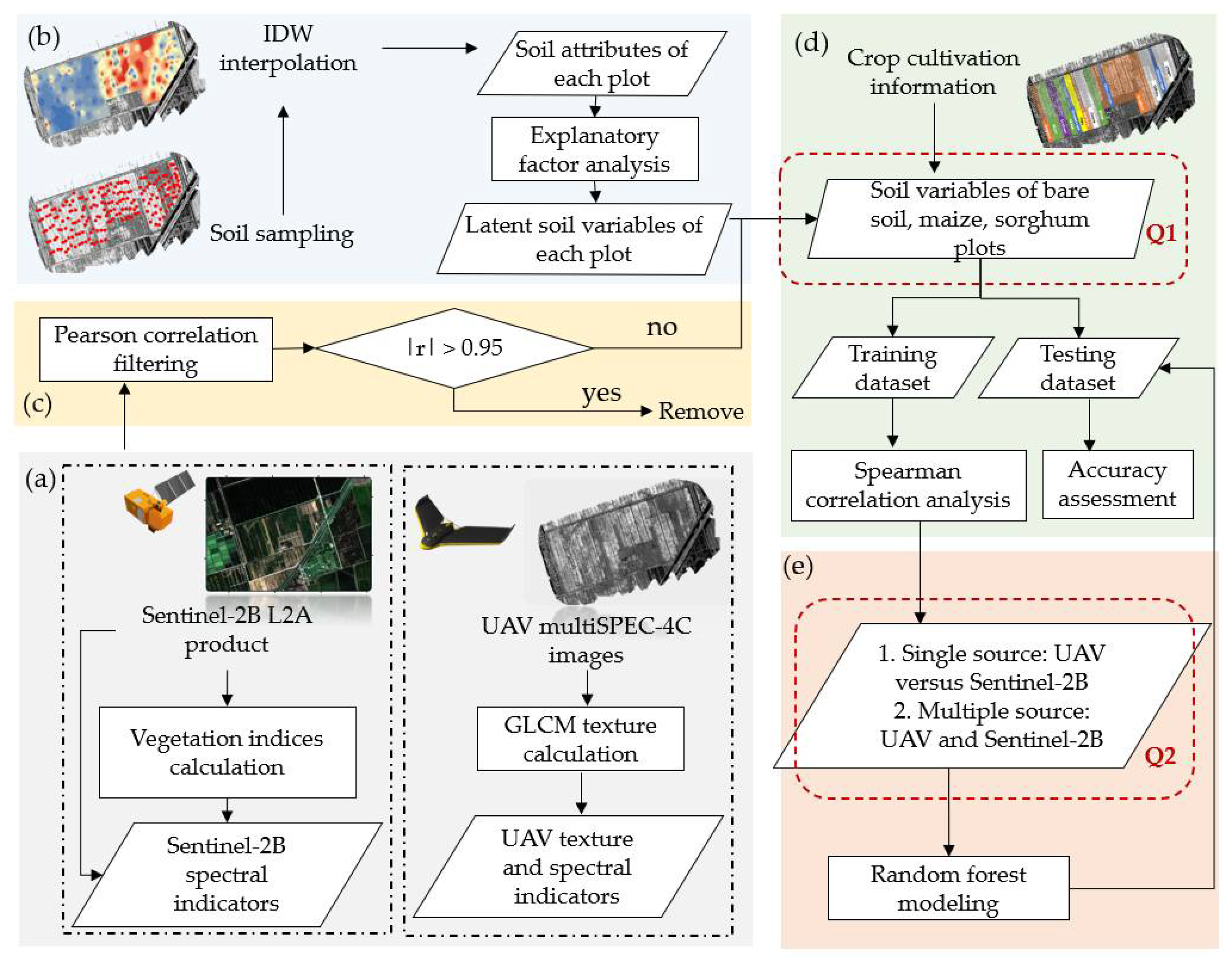
2.2. Overview of the Workflow in This Study

The workflow of this study includes four steps (Figure 2):

(a)

Generating remote sensing indicators, including UAV texture/spectral and Sentinel-2B spectral indicators, and investigating the difference between UAV and Sentinel-2B similar bands (Section 2.3.1, Section 2.3.2, Section 2.3.3);

(b)

Conducting the exploratory factor analysis to generate soil latent variables that could effectively reflect the variance of soil fertility and salinity (Section 2.4);

(c)

Conducting the Pearson correlation filtering to remove highly correlated remote sensing indicators when the |r| values are over 0.95 (Section 2.5.1);

(d)

Dividing the study area into three regions covered by the bare soil, maize, and sorghum, then conducting the Spearman correlation analysis to identify informative remote sensing indicators for the soil variable estimation (Section 2.5.2);

(e)

Running the random forest model to estimate soil variables using remote sensing indicators, comparing the performance of single- (UAV versus Sentinel-2B) and multi-source remote sensing data, investigating whether the integration of spectral and texture data could lead to a better estimation (research question 2), and comparing the soil variable estimation accuracy of places with different coverage—bare soil, maize, and sorghum (research question 1) (Section 2.5.3).

2.3. Acquisition and Processing of Remote Sensing Data

2.3.1. Acquisition and Pre-Processing of UAV Remote Sensing Data

UAV flight missions were executed on 17 August 2019. An eBee wing-fixed UAV platform (SenseFly, S.A., Lausanne, Switzerland) equipped with a multiSPEC-4C multispectral camera (SenseFly, S.A., Lausanne, Switzerland) was employed to collect images. The multiSPEC-4C has four separate channels centered at 550 nm (green), 660 nm (red), 735 nm (red edge), and 790 nm (the near-infrared (NIR) band), with bandwidths of 40 nm, 40 nm, 10 nm, and 40 nm, respectively (Figure 3). As the experimental site was large, three UAV flight missions were conducted between 10:00–14:00 with a clear sky and low wind; the shooting time lasted 1.5 h. The flight heights for three missions were 150 m, with spatial resolution around 0.20 m. The reflectance of spectral panels was photographed before each flight for the next radiation calibration. UAV images were captured with the camera pointing in the nadir (0°) direction. UAV flight was controlled using the proprietary eMotion 3 software (Pix4D, S.A., Lausanne, Switzerland). The Pix4D Mapper (Pix4D, S.A., Lausanne, Switzerland) was used for radiation calibration and generation of UAV orthography.

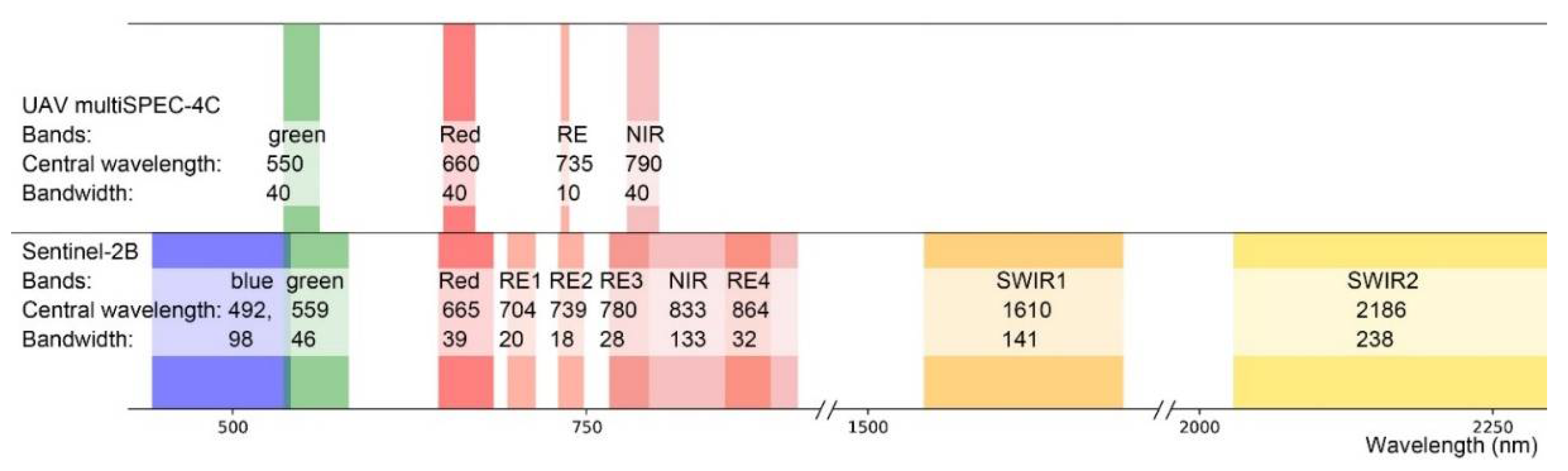
2.3.2. Acquisition and Preprocessing of Sentinel-2 Data

The Sentinel-2B L1C product from 17 August 2019 was downloaded from the website https://earthexplorer.usgs.gov/ (accessed on 12 July 2021), which has been geometrically calibrated. The Sen2Cor was used for the radiation calibration of L1C products to generate the L2A products. The L2A products with a ground spatial resolution of 20 m were used for further analysis. Sentinel-2B sensor has 13 bands, 10 of which were selected for this study while considering the spatial resolution and central wavelength, including bands 2, 3, 4, 5, 6, 7, 8, 8a, 11, and 12, denoted as blue, green, red, red edge1 (RE1), RE2, RE3, NIR, RE4, Short-wave infrared (SWIR1), and SWIR2, respectively (Figure 3).

2.3.3. Generation and Extraction of Remote Sensing Indicators

As the UAV images have a high spatial resolution, these data were used to calculate the canopy texture using the grey level co-occurrence matrix (GLCM) [31] via the r.texture tool of the QGIS open-source software. In total, 13 texture variables were calculated; the first-order statistics in the spatial domain calculated 7 variables—sum average (sa), entropy (ent), difference entropy (de), sum entropy (se), variance (var), difference variance (dv), and sum variance (sv); and the second-order statistics calculated 6 variables—angular second moment (asm), inverse difference moment (idm), contrast (con), correlation (cor), information measures of correlation (moc), and maximal correlation coefficient (mcc). Since the UAV images have four bands, 13 × 4 (UAV bands) = 52 texture variables were generated.

Spectral variables included the reflectance of bands and VIs. Both UAV and L2A band reflectance remained, while the calculation of VIs (

Table 1. Vegetation indices were used in this study.

Forms 1	Names of Vegetation Indices	Formulas 2	References
(b1 − b2)/(b1 + b2)	Normalized Difference Vegetation index	NDVI = (NIR − R)/(NIR + R)	[37]
	Red edge NDVI	NDREij 1 = (REi − REj)/(REi + REj)	[38]
	Green NDVI	GNDVI = (NIR − G)/(NIR + G)	[39]
b1/b2	Simple Ratio	SR = NIR/G	[39]
	Red edge reflectance ratio	PRij = REi/REj	[37]
	Ratio vegetation index	RVI = NIR/R	[38]
b1 − b2	Reflectance difference	RD = NIR − R	[37]
	Red edge reflectance difference	REDi = REi − B
(b1 − b2)/b3	Plant senescence reflectance index	PSRIi = (R − B)/REi	[40]
	Chlorophyll index green	CIG = (REi − G)/G
	Red Edge Relative Indices	RERIi = (REi − R)/NIR
Hybrid	Transformed Chlorophyll Absorption in Reflectance Index	TCARI = 3[(RE1 − R) − 0.2(RE1 – G)(RE1/R)]	[41]
	Optimized soil adjusted vegetation index	OSAVI = 1.16(NIR − R)/(NIR + R + 0.16)
	Enhanced Vegetation Index	EVI = 2.5 ((NIR−R)/(NIR + 6R − 7.5B + 1))	[42]
	Improved chlorophyll absorption ratio index	MCARI = (RE1 − R) − 0.2(RE1 − G)(RE1/R)	[39]
	Red-edge vegetation stress index	RVSI = [(RE1 + RE3)/2] − RE2	[43]
	Modified simple ratio	MSR = $\left(\mathrm{NIR}/\mathrm{R}-1\right)/\sqrt{\mathrm{NIR}/\mathrm{R}-1}$	[38]
	Modified simple ratio Red-edge	MSRRE = $\left(\mathrm{NIR}/{\mathrm{RE}}_1-1\right)/\sqrt{\mathrm{NIR}/{\mathrm{RE}}_1-1}$	[44]

¹b_i represents the reflectance of band i. ² B, G, R, RE1, RE2, RE3, NIR, and RE4 are the reflectance of Sentinel-2B bands 2, 3, 4, 5, 6, 7, 8, and 8a, respectively.

, using Python 3.7) was based on the L2A data because the Sentinel-2B sensor has more spectral bands (visible-NIR-SWIR) than the UAV multiSPEC-4C camera (only four bands).

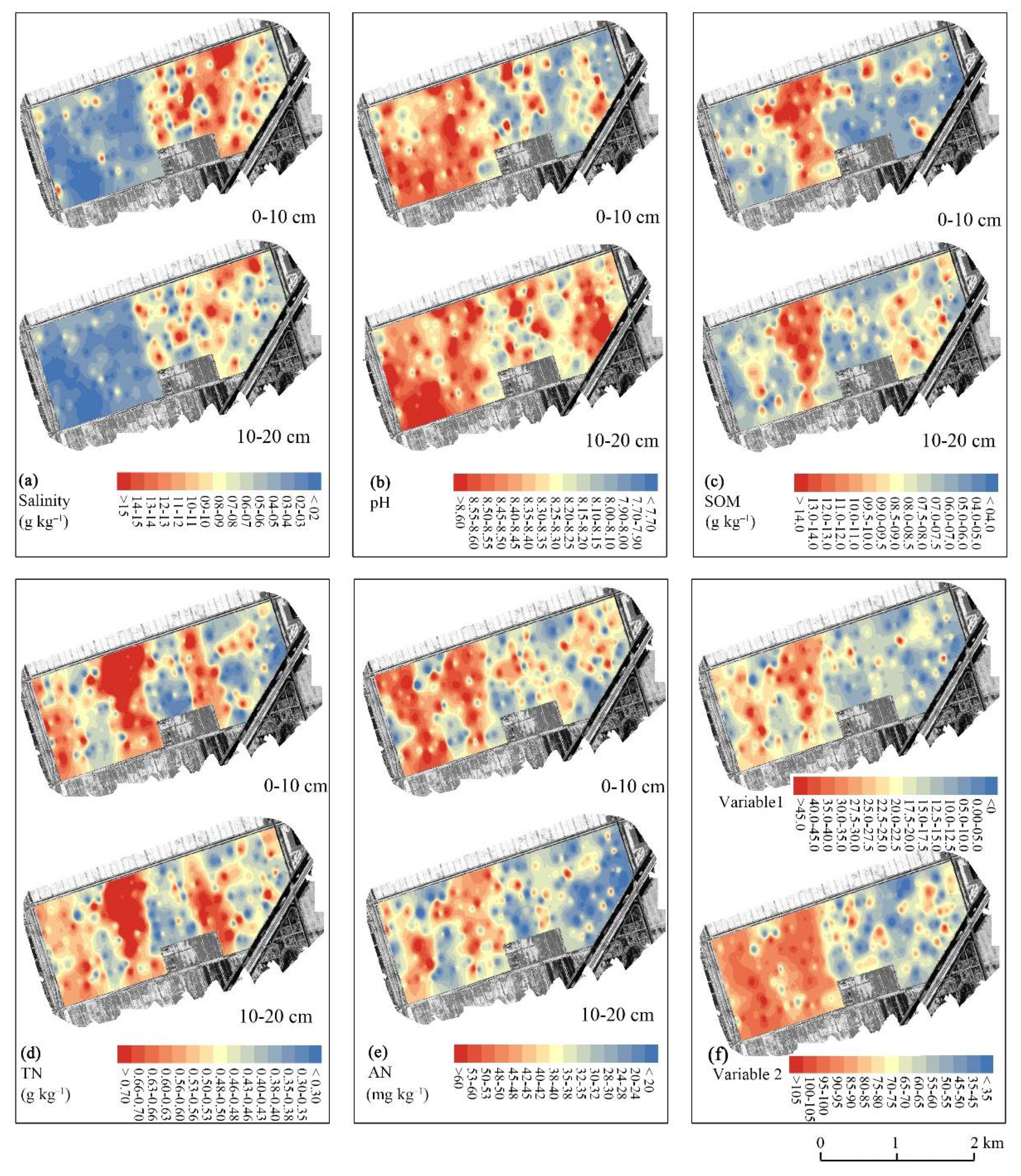
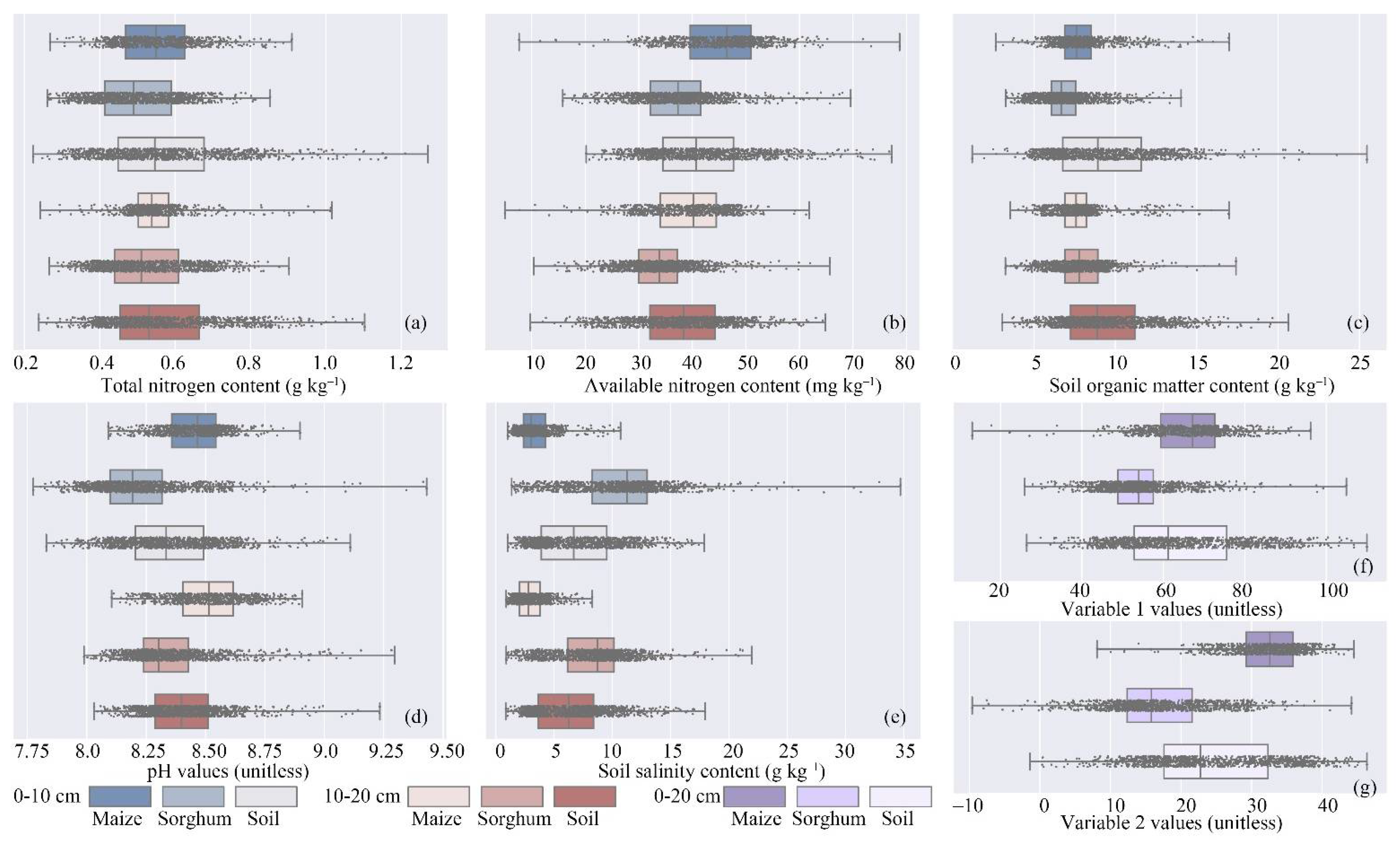
2.4. Collection and Processing of Soil Data

2.4.1. Ground Measurements

Soil sampling was conducted along the strip field and evenly distributed to cover the study area on 15 August 2019 (two days before the UAV flight). In total, 195 sampling points were collected. The location of each sample point was recorded by Android smartphone MI 8 GPS (Xiaomi Technology Co., Ltd., Beijing, China). In this study, five soil attributes at 0–10 cm and 10–20 cm layers were measured, including the soil salinity content (g kg⁻¹), soil organic matter content (SOM, g kg⁻¹), total nitrogen content (TN, g kg⁻¹), available nitrogen content (AN, mg kg⁻¹), and pH. In order to match the soil and remote sensing data in space, the inverse distance weighted (IDW) spatial interpolation, which has been widely applied in soil interpolation [14], was conducted to obtain the spatial variations of soil attributes (Figure 4). Considering the spatial resolutions of L2A products, a 20 m × 20 m plot was set as a sample size. The mean values of all pixels within each plot were calculated to represent the plot-level values using the QGIS. In total, the experimental site was divided into 4797 plots; the numbers of bare soil, sorghum, and maize plots were 1182, 1219, and 811, respectively. The statistical characteristics of soil attributes and latent variables for these three regions are shown in Figure 5. Soil attributes and variables are called soil indicators hereafter.

2.4.2. Explanatory Factor Analysis of Soil Attributes

Since crop growth was affected by comprehensive soil conditions, the explanatory factor analysis [13] was conducted to reduce the number of variables using the psych package in the R 3.6.3 software. The Parallel analysis showed that the number of variables should be set to 2 (Figure S1). Then, the orthogonal rotation was used to extract variables. As shown in

Table 2. Results of the explanatory factor analysis for soil attributes.

		PA1 2	PA2	h2 3	u2 4
Soil attributes 1	salinity 0–10 cm	−0.26	−0.87	0.83	0.17
	salinity 10–20 cm	−0.18	−0.89	0.82	0.18
	SOM 0–10 cm	0.81	0.08	0.67	0.33
	SOM 10–20 cm	0.82	−0.07	0.67	0.33
	TN 0–10 cm	0.85	0.15	0.75	0.25
	TN 10–20 cm	0.84	0.13	0.72	0.28
	AN 0–10 cm	0.56	0.34	0.44	0.56
	AN 10–20 cm	0.71	0.21	0.54	0.46
	pH 0–10 cm	0.09	0.84	0.71	0.29
	pH 10–20 cm	0.00	0.80	0.64	0.36
Cumulative variation		0.37	0.68
Proportion explained		0.54	0.46

¹ SOM, soil organic matter content, g kg⁻¹; TN, soil total nitrogen content, g kg⁻¹; AN, soil available nitrogen content mg kg⁻¹. ² PA is the correlation coefficient between observed attributes and variables. ³ h2 is the common variable variance, i.e., the degree of methodological explanation of each variable by variables. ⁴ u2 = 1−h2 denotes the proportion of variance that cannot be explained by variables.

, the first and most important latent variable (Variable 1, calculated via the PA1 results) explained 37% of the total variance; Variables 1 and 2 (calculated via the PA2 results) collectively accounted for 68% of the total variance. Variable 1 had the largest eigenvalue, with high loadings for SOM, AN, and TN (>0.5), so Variable 1 was termed the fertility variable. Variable 2 was termed the salinity and sodicity variable because of the high loadings for salinity and pH (>0.8). Further steps applied remote sensing information to estimate Variables 1 and 2.

2.5. Screening of UAV Variables and Modeling for Soil Latent Variable Estimation

2.5.1. Filtering Highly Correlated Remote Sensing Indicators

In order to mitigate multi-collinearity issue, the Pearson correlation analysis was carried out for filtering highly correlated remote sensing variables (|r| > 0.95, p < 0.01, n = 4797) by executing the findCorrelation functions in the caret package of R [20]. After filtering, 17 spectral (i.e., UAV-g, UAV-r, UAV-e, UAV-nir, RE1, RE2, NIR, SWIR1, SWIR2, PR42, PR43, PR32, ratio vegetation index (RVI), red-edge reflectance difference 1 (RED1), red edge relative indices 1 (RERI1), RERI2, and transformed chlorophyll absorption in reflectance index (TCARI)) and 14 texture (i.e., g-con, g-cor, g-de, g-dv, g-idm, g-mcc, g-sa, g-sv, r-cor, r-de, r-dv, r-se, r-sv, and r-var.) variables remained. The g, r, e, and nir represent the green, red, red edge, and the near-infrared bands-based UAV variables, respectively.

2.5.2. Spearman Correlation Analysis

The Spearman’s rank correlation coefficient (denoted as ρ) [45] was used to quantify the correlation between soil indicators and remote sensing indicators, where the correlation between the variables can be described using a monotonic function. The range of ρ values is between +1 and −1, denoting positive and negative relationships, respectively, and higher values of |ρ| represent the strong correlations. This process aimed to identify vital remote sensing indicators for soil variable estimation, executed in R 3.6.3.

2.5.3. Modeling and Accuracy Assessment

In this study, a typical machine-learning method, random forest, was used for modeling via the randomForest R package. The random forest model includes two key parameters, mtry and ntree. The mtry was set to 3 (default value), and the optimal ntree values were determined by the minimum error. A three-fold cross-validation approach was used for model calibration and validation. Model estimation accuracy was evaluated using the coefficient of determination (R²), root mean square error (RMSE), and mean absolute percentage error (MAPE, %) as:

$$R^2={\{[{{\displaystyle \sum }}_{i=1}^n\left(M_i-\overline{M}\right)\left(E_i-\overline{E}\right)]/[\sqrt{{{\displaystyle \sum }}_{i=1}^n{\left(M_i-\overline{M}\right)}^2}\sqrt{{{\displaystyle \sum }}_{i=1}^n{\left(E_i-\overline{E}\right)}^2}]\}}^2$$

(1)

$$\mathrm{RMSE}=\sqrt{{{\displaystyle \sum }}_{i=1}^n{\left(M_i-E_i\right)}^2/n}$$

(2)

$$\mathrm{MAPE}=({\displaystyle \sum }_{i=1}^n\left|M_i-E_i\right|)/M_i$$

(3)

where i is the sequence number of the sample, M_i is the calculated soil latent variable values, E_i is the estimated soil variable values, $\overline{M}$ represents the average value of the calculated soil latent variable array, and $\overline{E}$ represents the average value of the estimated soil latent variable array.

3. Results

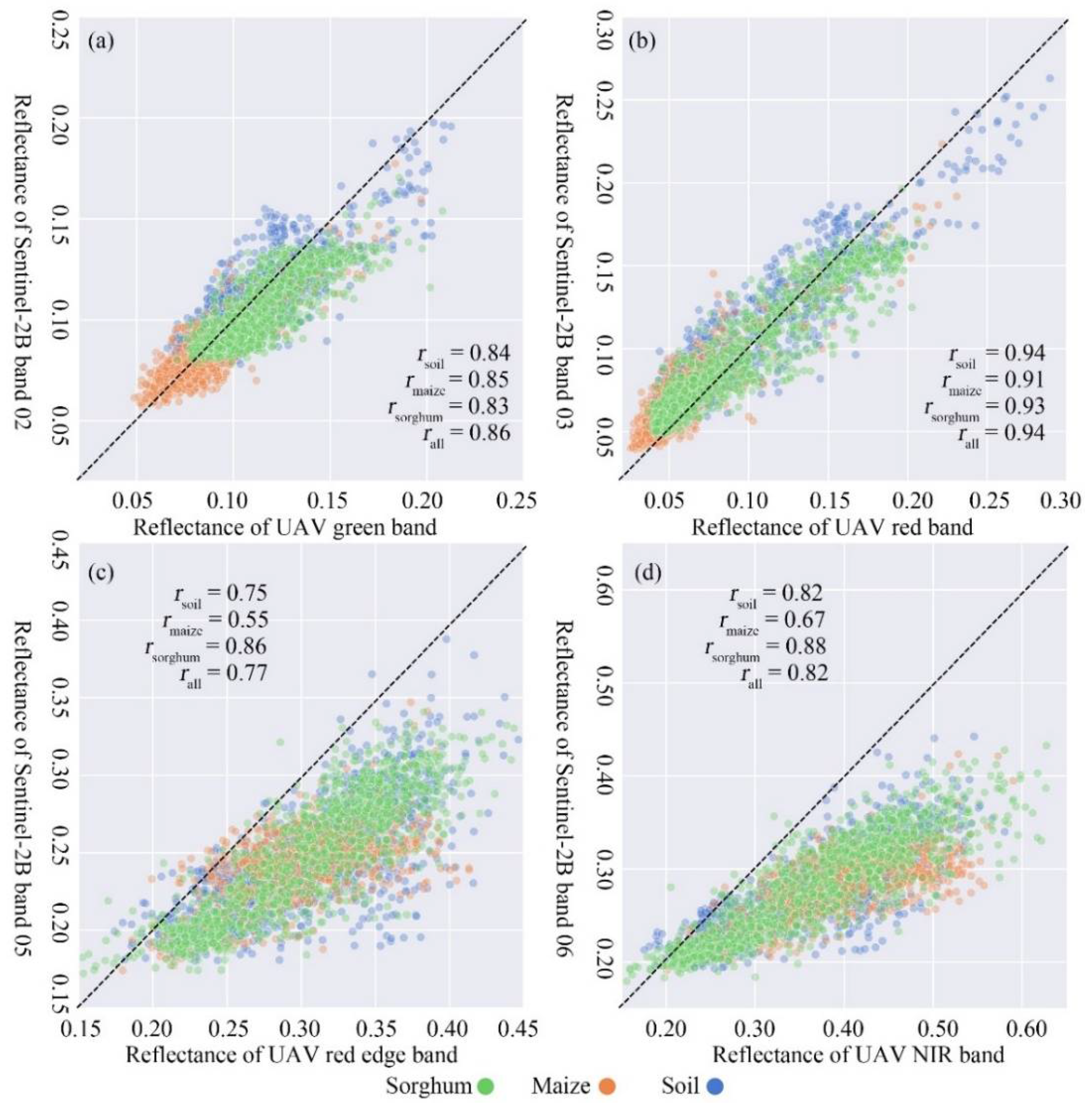
3.1. Relationships between UAV and Sentinel-2B Reflectance

The reflectance of UAV and Sentinel-2B bands with a similar central wavelength, i.e., UAV green versus Sentinel 02, UAV red versus Sentinel 03, UAV red edge versus Sentinel 05, and UAV nir versus Sentinel 06 bands, is compared in Figure 6. The one-to-one reflectance at the plot level exhibits a significantly positive linear correlation with r_all values of 0.77–0.94 (n = 3212, p < 0.001), suggesting that the average values of all UAV pixels within each plot can appropriately represent the plot-level Sentinel-2B-based information of ground objects. However, these relationships differ for distinct bands; the r_all value of red bands is 0.94, higher than other bands; and the r_all values of red edge bands is 0.77. This result indicates that the transfer of UAV-calibrate models might introduce uncertainties in satellite-based applications. Besides, the coverage of ground does not affect the relationships between the reflectance of similar UAV and Sentinel-2B bands significantly, as the r values of soil, maize, and sorghum plots are comparable.

3.2. Relationships between Remote Sensing Indicators and Soil Indicators

The relationships between remote sensing indicators and soil indicators were different at different plots (Figure 7), and the sorghum region exhibited the highest |ρ| values, remarkably higher than the maize and bare soil regions. In particular, at the bare soil (n_soil = 1182), UAV variables with the high |ρ| values were g-sa (ρ_PA1 = −0.22, ρ_PA2 = −0.18, p < 0.001), g-sv (ρ_PA1 = −0.20, ρ_PA2 = −0.15, p < 0.001), and UAV-g (ρ_PA1 = −0.23, ρ_PA2 = −0.21, p < 0.001). At maize plots (n_maize = 811), the highest |ρ| values were seen for g-dv (ρ_PA1 = −0.31, ρ_PA2 = −0.28) and g-idm (ρ_PA1, ρ_PA2 = −0.22). As for Sentinel-2B variables, at the bare soil, SWIR1 (ρ_PA1 = 0.27, ρ_PA2 = 0.34) and SWIR2 (ρ_PA1 = 0.16, ρ_PA2 = 0.22, p < 0.001) had the highest |ρ| values, while at maize plots, the RERI1 had the highest values (ρ_PA1 = 0.68, ρ_PA2 = 0.57, p < 0.001). Regarding sorghum plots, most UAV and Sentinel-2B variables indicated high |ρ| values, suggesting that many remote sensing indicators of sorghum plots were highly correlated with ground-based soil indicators. The UAV and Sentinel-2B variables with the top five |ρ| values are listed in

Table 3. Remote sensing indicators used for soil variable estimation.

Regions	Soil Variables	UAV Indicators	Sentinel-2B Indicators
Bare soil	Variable 1	UAV-g, g-sa, g-sv, UAV-e, r-var	RERI1, RE1, RED1, SWIR2, SWIR1
	Variable 2	UAV-g, g-sa, UAV-e, g-sv, r-dv	RVI, PR43, RED1, SWIR2, SWIR1
Sorghum	Variable 1	UAV-r, r-sv, UAV-e, UAV-nir, UAV-g	SWIR2, RE2, RVI, RERI2, TCARI
	Variable 2	UAV-r, r-sv, UAV-e, UAV-nir, g-mcc	RERI2, TCARI, RERI1, RE2, RVI
Maize	Variable 1	g-dv, g-idm, g-de, g-mcc, g-con	NIR, PR32, PR42, TCARI, RERI1
	Variable 2	g-dv, g-idm, g-con, g-mcc, g-de	NIR, PR32, RERI1, TCARI, RED1

, and these variables are used for the following estimation of soil attributes.

Compared to the |ρ| values of soil indicators, overall, fertility-related indicators, such as Variable1, AN, and TN, showed higher |ρ| values than the salinity and sodicity indicators (i.e., salinity, pH, and Variable 2). This suggests that the estimation accuracy of soil nutrition indicators might be higher than the estimation of salinity and sodicity indicators. When comparing soil attributes and latent variables, their |ρ| values were comparable at the bare soil region, while the soil variables exhibited slightly higher |ρ| values at the maize region and the highest at the sorghum region. This result indicated that the estimation of soil latent variables based on remote sensing might be more accurate than the estimation of a single soil attribute.

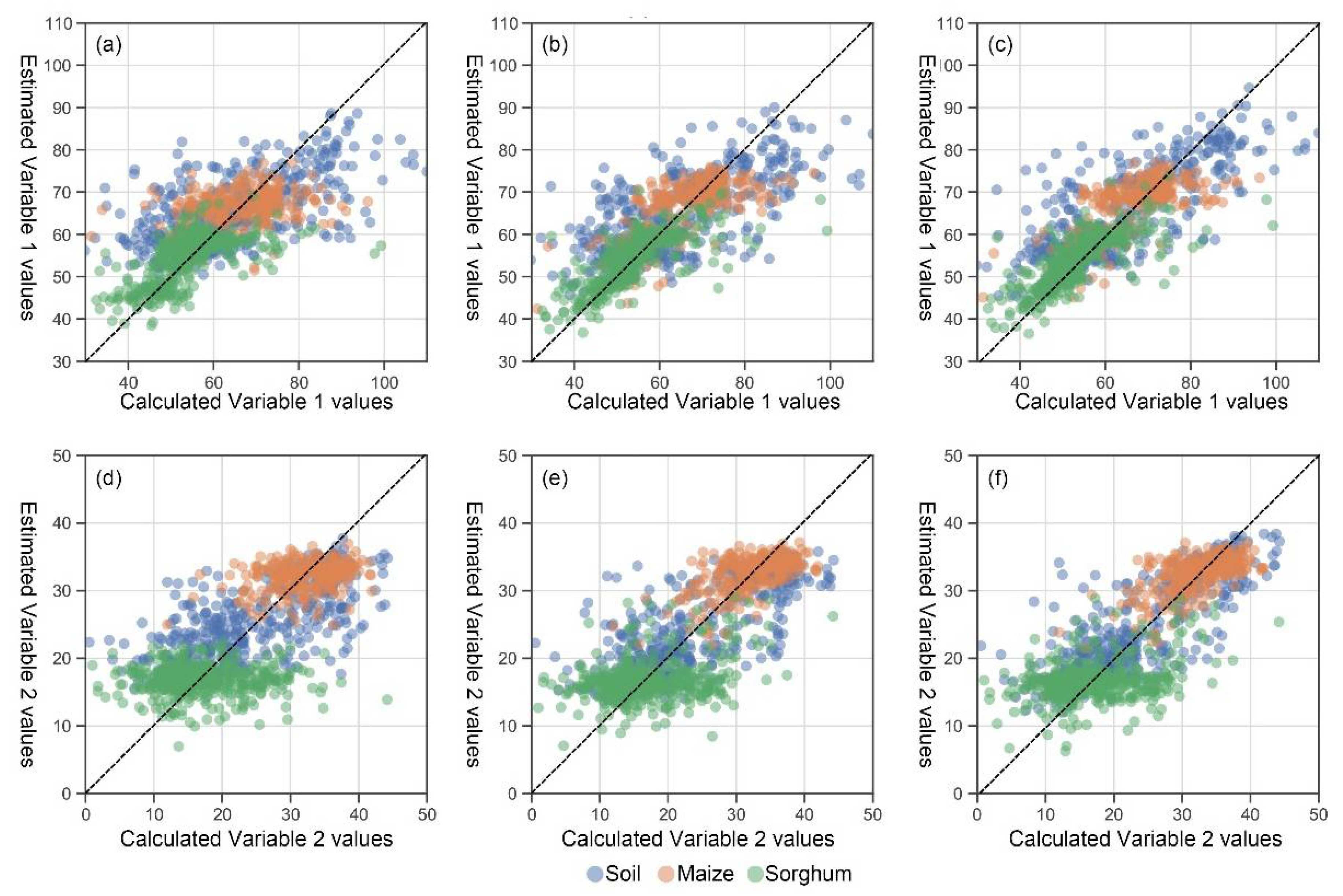
3.3. Estimation of Soil Variables Using Remote Sensing Indicators

Processing remote sensing data without classification of the land use indicated that the R² and MAPE values of Variable 1 estimation were 0.44–0.63 and 9.62–12.22%, respectively, while those two of Variable 2 estimation were 0.51–0.65 and 27.79–33.46%, respectively (

Table 4. Estimation accuracy assessment of soil latent variables using different remote sensing indicators.

Soil Latent Variables	Regions	R2			RMSE			MAPE (%)
		UAV	L2A 1	Inte. 2	UAV	L2A	Inte.	UAV	L2A	Inte.
Variable 1	Bare soil	0.38	0.45	0.57	12.21	11.48	10.13	15.91	15.12	12.93
	Sorghum	0.37	0.54	0.54	6.97	5.95	5.99	9.09	7.03	7.12
	Maize	0.12	0.48	0.49	9.18	7.04	7.01	11.55	8.58	8.59
	All	0.44	0.56	0.63	9.72	8.62	7.98	12.22	10.39	9.62
Variable 2	Bare soil	0.40	0.51	0.64	7.15	6.45	5.57	41.81	37.85	33.86
	Sorghum	0.01	0.11	0.13	7.27	6.61	6.55	39.39	34.75	33.76
	Maize	0.09	0.35	0.37	4.61	3.88	3.80	12.50	10.33	10.08
	All	0.51	0.60	0.65	6.65	5.97	5.60	33.46	29.69	27.79

¹ L2A = Sentinel-2B L2A data. ² Inte. = Integration of Sentinel-2B L2A and UAV remote sensing indicators.

and Figure 8). These results revealed that the estimation accuracy of soil latent fertility variable using remote sensing data was more accurate than the estimation of salinity and sodicity variable, which is consistent with the Spearman correlation analysis.

When dividing into different land covers, regarding the Variable 1 estimation, the R², RMSE, and MAPE values of the bare soil were 0.38–0.57, 10.13–12.21, and 12.93–15.91%, respectively; the three values of the maize were 0.12–0.49, 7.01–9.18, and 8.58–11.55%, respectively; and at the sorghum region, they were 0.37–0.54, 5.95–6.97, and 7.03–9.09%, respectively (Table 4). In terms of the Variable 2 estimation, the R², RMSE, and MAPE values of soil plots were around 0.50, 6.50, and 37%, respectively (Table 4). The three values were 0.10, 6.50, and 35% of sorghum region, and 0.30, 4.0, and 10% of maize plots. The abovementioned results revealed that the type of land cover could affect the accuracy of soil attribute estimations. The accuracy of soil Variable 1 estimation was in the order of sorghum > maize > soil, while the maize region exhibited the highest estimation accuracy of Variable 2, and those of sorghum and bare soil region were comparable. Overall, it could be concluded that the estimation of soil variables using crop-covered regions exhibited better accuracy than the bare soil region.

Comparing the estimation accuracy of different remote sensing datasets, for single-source data, the Sentinel-2B outperformed the UAV data for both variable estimations. Furthermore, the integration of Sentinel-2B data into UAV-based observations remarkably improved the accuracy of estimations for soil variables compared to only UAV estimations, particularly for maize plots. However, the availability and quality of the satellites and timing overlap between UAV campaigns and satellite-based information can limit the potential of integrations.

4. Discussion

In the current study, we used UAV multispectral and Sentinel-2B sensing information for the estimation of soil fertility and salinity over a large agricultural farm consisting of croplands and fallow lands. Our findings revealed that the reflectance of UAV multiSPEC-4C and Sentinel-2B in similar central wavelengths exhibited strong linear relationships while differing for distinct bands. The estimation accuracy of latent soil variables using remote sensing data for croplands was higher compared to the harvested lands; the integration of UAV texture and Sentinel-2B spectral data improved the estimation accuracy of latent soil variables.

4.1. Factors Affecting the Relationships between UAV and Sentinel-2B Reflectance

The Pearson correlation analysis showed that the UAV and Sentinel-2B reflectance yielded a significant correlation, meaning both sources of information can detect the variations in soil attributes. It should be noted that this relationship was stronger for green and red bands compared to the red edge band. Remote sensing reflectance is sensor-dependent [19]. The channel design of UAV multiSPEC-4C and Sentinel-2B multispectral sensors differed in central wavelength and bandwidth. As shown in Figure 3, the overlap of UAV red edge and Sentinel RE2 bands was less than the other three bands, so the reflectance of these two bands exhibited the lowest correlations. Further, the bandwidth of the RE channel was very narrow (10 nm), so the signal of this band was not strong enough and therefore might be more easily affected by environmental conditions [46]. Another argument could be that the reflectance at the red edge and NIR ranges usually changed rapidly [30], so the slight difference in central wavelengths and bandwidths could cause an obvious discrepancy in reflectance.

The comparable reflectance of UAV and Sentinel-2B bands revealed that the average of all UAV remote sensing pixels within a plot could effectively represent the plot level information captured by satellite remote sensing when their sensors have a similar specification, which is an important prerequisite for the combination of UAV and satellite remote sensing, particularly in the ‘UAV-calibrated and satellite-validated’ approach. Otherwise, the difference between UAV and satellite reflectance might cause many uncertainties and biases on the performance of estimation. Other factors, such as the difference in spatial resolution of these two data sources, as well as the spatial heterogeneity of observed objects, would affect the relationships between UAV and satellite bands. Future studies could further investigate these mentioned issues.

4.2. Factors Affecting the Performance of Soil- and Crop-Based Remote Sensing Approaches

The results of this study showed that the land cover affected the accuracy of estimating soil attributes, and, overall, the crop-based approach exhibited higher accuracy than the soil-based approach. This can be explained by the fact that crops played a ‘signal amplification’ role in soil attributes, and it is easier to capture crop features than soil features under satellite and aerial observations. Nonetheless, the soil-based way is not affected by crop phenology, and our study also demonstrated that this approach is feasible for soil latent variable estimation.

This study estimated the latent soil variables instead of a single soil attribute. Previous studies have successfully conducted the estimation of single soil attributes (e.g., salinity and SOM) via remote sensing [47]. However, it should be noted that most of them were conducted using hyperspectral sensors with ultrahigh spectral (~2 nm) and spatial resolutions (mm level) [27,48]. The satellite and aerial images can obtain a large coverage, but a low degree of spectral and detailed spatial information tends to limit interpretation for the qualitative determination of soil attributes [49]. On the other side, the spatial variance of fertility and salinity in this region remained largely uncertain. Remotely sensed information of soil and crops is affected by multiple soil attributes. Different soil attributes might lead to similar remotely sensed information, but it is difficult to identify based on the limited spatial and spectral resolutions. In such a context, the estimation of soil latent variables and comprehensive indicators is more effective. Finally, such detection of soil latent variables could be a quick approach for targeting soil comprehensive conditions at the field scale, which is vastly helpful for agronomic management. Besides, crop nitrogen content can be linearly explained by soil nitrogen levels due to the role of nitrogen in leaf area expansion [50], which could partially explain that the estimation accuracy of ‘fertility’ (Variable 1), which was higher than the ‘salinity and sodicity’ (Variable 2).

Comparing two crop plots of sorghum and maize for soil variables estimation revealed that the sorghum plots yielded higher accuracy in the Variable 1 estimation, while this was the case for maize with Variable 2 estimation. However, it is challenging to disentangle the main driver of the difference between crops since maize and sorghum were cultivated in places with distinct soil conditions. Future studies should conduct controlled experiments to further investigate this phenomenon. Furthermore, although more remote sensing indicators in the sorghum plots had higher |ρ| values than those in the maize plots, the estimation accuracy in sorghum and maize regions was comparable. We inferred this could be owing to the different phenological phases at the time of the observations and the differences in the response of maize and sorghum canopies to different levels of salinity and soil nutrients. Although the sowing dates of maize and sorghum were close, their growth rates were different; maize was at the late grain filling stage, while sorghum was at the early grain filling stage during the observation campaign. The color of maize leaves at the terminal growth stage may be less representative of the nutritional condition of the soil, which was not the case for sorghum in this experiment. Therefore, single remote sensing indicators might not be sufficient to characterize the representative status of maize at the late grain-filling stage. The integration of texture and spectral variables provided abundant information of crops so that the soil variable estimation of maize plots could achieve satisfying accuracy.

In addition, it is commonly recognized that 95% of all roots are in the upper 2 m soil layer. Roots play a fundamental role in nutrient and water uptake for supporting crop growth [51]. The proportion of crop root biomass significantly differed for distinct regions. Generally, the distribution of crop roots is affected by potential evapotranspiration, precipitation, and the length of the warm season; and deeper rooting depths were mainly found in arid ecosystems [52]. As earlier mentioned, this study was conducted at a coastal saline land with a shallow groundwater table and flat terrain [34], close to the Bohai Sea (~10 km). Maize and sorghum were planted during May and October when maritime climate with abundant rainfall and warm temperature is prevalent. In addition, soil properties, such as texture, bulk density, fertility, and agronomic management (e.g., fertilizer placement and tillage) influence crop root traits [53]. The study area is formed by the Yellow River sediment, which has a short time of reclamation (≤2 years). The long-term upward salt return from seawater leads to the severe saline of this region, thus causing soil consolidation and hindering the penetration of crop roots [54]. Under the effects of the above comprehensive factors, the root distribution at the experimental site should be shallow. The study of Wang et al. (2018) also proved that maize cultivated close to the experimental site (with less saline) exhibited around 70% root biomass at a 0–20 cm layer [53]. Some studies have demonstrated that nitrogen fertilizer significantly affected root traits only in the top 30 cm of the soil layer [54]. Under this circumstance, the 0–20 cm soil layer dominantly affected crop growth, and the soil characteristics can be translated into remotely sensed reflectance from crop surface; thus, the comparison of soil-based and crop-based approaches in this study is adequate. On the other hand, we would like to highlight that optical remote sensing is not suitable to penetrate the soil profile, so deeper soil variable estimation might not be appropriate for the soil-based method.

4.3. Factors Affecting the Performance of Distinct Remote Sensing Data Source

The Sentinel-2B dataset included spectral variables, while the UAV dataset mainly contained texture variables. Even though the spatial resolution of UAV images (0.20 m) was significantly higher than the Sentinel-2B products (20 m), the Sentinel-2B data provided more spectral information, particularly in the red-NIR range, which is sensitive to crop features [30,44,55]. Besides, spectral information might be more informative than texture variables because spectral variables are affected by both biochemical and structural features of crops, while texture variables are likely mainly influenced by crop structure. The higher |ρ| values of spectral variables can also support this explanation. Therefore, the Sentinel-2B data outperformed the UAV data for soil variable estimation. This study did not calculate VIs using UAV data, nor did it compare the performance of UAV and Sentinel-2B spectral information regarding soil variable estimation. We focused more on the integration of UAV and satellite data to make use of the complete advantages of UAV high spatial resolution and Sentinel-2B abundant spectral information to improve soil salinity and fertility estimation accuracy.

5. Conclusions

This study used UAV multispectral and Sentinel-2B data for the estimation of soil latent variables considering salinity and fertility over large agricultural land consisting of cropland (maize and sorghum) and harvest area (bare soil). Our results revealed that the integration of UAV texture and Sentinel-2B spectral data improved the estimation accuracy of latent soil variables. The remote sensing data covered by crops resulted in higher accuracy compared to estimations performed on the bare soil. Thus, the crop-based approach, along with the integration of UAV texture and Sentinel-2B data, is recommended for the quick assessment of soil comprehensive attributes. This study contributes to the multi-source remote sensing-based detection of soil comprehensive salinity and fertility conditions, vastly helpful for the field-scale agronomic management.

References

1. Che, Z.; Wang, J.; Li, J. Effects of water quality, irrigation amount and nitrogen applied on soil salinity and cotton production under mulched drip irrigation in arid Northwest China. Agric. Water Manag. 2021, 247, 106738. [Google Scholar] [CrossRef]
2. Sultana, S.; Alam, S.; Karim, M.M. Screening of siderophore-producing salt-tolerant rhizobacteria suitable for supporting plant growth in saline soils with iron limitation. J. Agric. Food Res. 2021, 4, 100150. [Google Scholar] [CrossRef]
3. Zhu, L.; Jia, X.; Li, M.; Wang, Y.; Zhang, J.; Hou, J.; Wang, X. Associative effectiveness of bio-organic fertilizer and soil conditioners derived from the fermentation of food waste applied to greenhouse saline soil in Shan Dong Province, China. Appl. Soil Ecol. 2021, 167, 104006. [Google Scholar] [CrossRef]
4. Chen, M.; Zhang, S.; Liu, L.; Wu, L.; Ding, X. Combined organic amendments and mineral fertilizer application increase rice yield by improving soil structure, P availability and root growth in saline-alkaline soil. Soil Tillage Res. 2021, 212, 105060. [Google Scholar] [CrossRef]
5. Zhang, H.; Hobbie, E.A.; Feng, P.; Zhou, Z.; Niu, L.; Duan, W.; Hao, J.; Hu, K. Responses of soil organic carbon and crop yields to 33-year mineral fertilizer and straw additions under different tillage systems. Soil Tillage Res. 2021, 209, 104943. [Google Scholar] [CrossRef]
6. Gong, H.; Li, Y.; Li, S. Effects of the interaction between biochar and nutrients on soil organic carbon sequestration in soda saline-alkali grassland: A review. Glob. Ecol. Conserv. 2021, 26, e01449. [Google Scholar] [CrossRef]
7. Wong, V.N.L.; Greene, R.S.B.; Dalal, R.C.; Murphy, B.W. Soil carbon dynamics in saline and sodic soils: A review. Soil Use Manag. 2009, 26, 2–11. [Google Scholar] [CrossRef]
8. Hurtado, A.C.; Chiconato, D.A.; Prado, R.D.M.; Junior, G.D.S.S.; Felisberto, G. Silicon attenuates sodium toxicity by improving nutritional efficiency in sorghum and sunflower plants. Plant Physiol. Biochem. 2019, 142, 224–233. [Google Scholar] [CrossRef]
9. Fu, Y.; Yang, G.; Pu, R.; Li, Z.; Li, H.; Xu, X.; Song, X.; Yang, X.; Zhao, C. An overview of crop nitrogen status assessment using hyperspectral remote sensing: Current status and perspectives. Eur. J. Agron. 2021, 124, 126241. [Google Scholar] [CrossRef]
10. Guan, Y.; Bai, J.; Wang, J.; Wang, W.; Wang, X.; Zhang, L.; Li, X.; Liu, X. Effects of groundwater tables and salinity levels on soil organic carbon and total nitrogen accumulation in coastal wetlands with different plant cover types in a Chinese estuary. Ecol. Indic. 2021, 121, 106969. [Google Scholar] [CrossRef]
11. Garcia-Caparros, P.; Llanderal, A.; Lao, M.T. Effects of salinity on growth, water-use efficiency, and nutrient leaching of three containerized ornamental plants. Commun. Soil Sci. Plant Anal. 2017, 48, 1221–1230. [Google Scholar] [CrossRef]
12. Zhu, H.; Yang, J.; Yao, R.; Wang, X.; Xie, W.; Zhu, W.; Liu, X.; Cao, Y.; Tao, J. Interactive effects of soil amendments (biochar and gypsum) and salinity on ammonia volatilization in coastal saline soil. Catena 2020, 190, 104527. [Google Scholar] [CrossRef]
13. Ayoubi, S.; Khormali, F.; Sahrawat, K.L. Relationships of barley biomass and grain yields to soil properties within a field in the arid region: Use of factor analysis. Acta Agric. Scand. Sect. B Plant Soil Sci. 2009, 59, 107–117. [Google Scholar] [CrossRef] [Green Version]
14. Nouri, H.; Borujeni, S.C.; Alaghmand, S.; Anderson, S.J.; Sutton, P.C.; Parvazian, S.; Beecham, S. Soil salinity mapping of urban greenery using remote sensing and proximal sensing techniques; The case of veale gardens within the adelaide parklands. Sustainability 2018, 10, 2826. [Google Scholar] [CrossRef] [Green Version]
15. Sishodia, R.P.; Ray, R.L.; Singh, S.K. Applications of remote sensing in precision agriculture: A review. Remote Sens. 2020, 12, 3136. [Google Scholar] [CrossRef]
16. Wang, D.; Chen, H.; Wang, Z.; Ma, Y. Inversion of soil salinity according to different salinization grades using multi-source remote sensing. Geocarto Int. 2020, 1–20. [Google Scholar] [CrossRef]
17. Ma, Y.; Chen, H.; Zhao, G.; Wang, Z.; Wang, D. Spectral index fusion for salinized soil salinity inversion using sentinel-2A and UAV images in a coastal area. IEEE Access 2020, 8, 159595–159608. [Google Scholar] [CrossRef]
18. Zhang, S.; Zhao, G. A Harmonious satellite-unmanned aerial vehicle-ground measurement inversion method for monitoring salinity in coastal saline soil. Remote Sens. 2019, 11, 1700. [Google Scholar] [CrossRef] [Green Version]
19. Soudani, K.; François, C.; le Maire, G.; Le Dantec, V.; Dufrêne, E. Comparative analysis of IKONOS, SPOT, and ETM+ data for leaf area index estimation in temperate coniferous and deciduous forest stands. Remote Sens. Environ. 2006, 102, 161–175. [Google Scholar] [CrossRef] [Green Version]
20. Zhu, W.; Sun, Z.; Huang, Y.; Yang, T.; Li, J.; Zhu, K.; Zhang, J.; Yang, B.; Shao, C.; Peng, J.; et al. Optimization of multi-source UAV RS agro-monitoring schemes designed for field-scale crop phenotyping. Precis. Agric. 2021, 22, 1768–1802. [Google Scholar] [CrossRef]
21. Dong, J.; Crow, W.T.; Tobin, K.J.; Cosh, M.H.; Bosch, D.D.; Starks, P.J.; Seyfried, M.; Collins, C.H. Comparison of microwave remote sensing and land surface modeling for surface soil moisture climatology estimation. Remote Sens. Environ. 2020, 242, 111756. [Google Scholar] [CrossRef]
22. Ramos, A.P.M.; Osco, L.P.; Furuya, D.E.G.; Gonçalves, W.N.; Santana, D.C.; Teodoro, L.P.R.; da Junior, C.A.S.; Capristo-Silva, G.F.; Li, J.; Baio, F.H.R.; et al. A random forest ranking approach to predict yield in maize with UAV-based vegetation spectral indices. Comput. Electron. Agric. 2020, 178, 105791. [Google Scholar] [CrossRef]
23. Weng, Y.-L.; Gong, P.; Zhu, Z.-L. A spectral index for estimating soil salinity in the yellow river delta region of China using EO-1 hyperion data. Pedosphere 2010, 20, 378–388. [Google Scholar] [CrossRef]
24. Chi, Y.; Shi, H.; Zheng, W.; Sun, J. Simulating spatial distribution of coastal soil carbon content using a comprehensive land surface factor system based on remote sensing. Sci. Total Environ. 2018, 628–629, 384–399. [Google Scholar] [CrossRef]
25. Xu, Y.; Wang, X.; Bai, J.; Wang, D.; Wang, W.; Guan, Y. Estimating the spatial distribution of soil total nitrogen and available potassium in coastal wetland soils in the Yellow River Delta by incorporating multi-source data. Ecol. Indic. 2020, 111, 106002. [Google Scholar] [CrossRef]
26. Ayub, M.; Ashraf, M.Y.; Kausar, A.; Saleem, S.; Anwar, S.; Altay, V.; Ozturk, M. Growth and physio-biochemical responses of maize (Zea Mays L.) to drought and heat stresses. Plant Biosyst. Int. J. Deal. All Asp. Plant Biol. 2021, 155, 535–542. [Google Scholar] [CrossRef]
27. Zhu, K.; Sun, Z.; Zhao, F.; Yang, T.; Tian, Z.; Lai, J.; Zhu, W.; Long, B. Relating hyperspectral vegetation indices with soil salinity at different depths for the diagnosis of winter wheat salt stress. Remote Sens. 2021, 13, 250. [Google Scholar] [CrossRef]
28. Song, C.; Ren, H.; Huang, C. Estimating soil salinity in the yellow river delta, eastern China—An integrated approach using spectral and terrain indices with the generalized additive model. Pedosphere 2016, 26, 626–635. [Google Scholar] [CrossRef]
29. De Almeida, C.T.; Galvão, L.S.; Aragão, L.E.D.O.C.E.; Ometto, J.P.H.B.; Jacon, A.D.; Pereira, F.R.D.S.; Sato, L.Y.; Pontes-Lopes, A.; Graça, P.; Silva, C.V.D.J.; et al. Combining LiDAR and hyperspectral data for aboveground biomass modeling in the Brazilian Amazon using different regression algorithms. Remote Sens. Environ. 2019, 232, 111323. [Google Scholar] [CrossRef]
30. Zhu, W.; Sun, Z.; Yang, T.; Li, J.; Peng, J.; Zhu, K.; Li, S.; Gong, H.; Lyu, Y.; Li, B.; et al. Estimating leaf chlorophyll content of crops via optimal unmanned aerial vehicle hyperspectral data at multi-scales. Comput. Electron. Agric. 2020, 178, 105786. [Google Scholar] [CrossRef]
31. Yue, J.; Yang, G.; Tian, Q.; Feng, H.; Xu, K.; Zhou, C. Estimate of winter-wheat above-ground biomass based on UAV ultrahigh-ground-resolution image textures and vegetation indices. ISPRS J. Photogramm. Remote Sens. 2019, 150, 226–244. [Google Scholar] [CrossRef]
32. Liu, G.; Li, J.; Zhang, X.; Wang, X.; Lv, Z.; Yang, J.; Shao, H.; Yu, S. GIS-mapping spatial distribution of soil salinity for Eco-restoring the Yellow River Delta in combination with Electromagnetic Induction. Ecol. Eng. 2016, 94, 306–314. [Google Scholar] [CrossRef]
33. Wu, C.; Liu, G.; Huang, C.; Liu, Q. Soil quality assessment in Yellow River Delta: Establishing a minimum data set and fuzzy logic model. Geoderma 2019, 334, 82–89. [Google Scholar] [CrossRef]
34. Zhu, W.; Yang, J.; Yao, R.; Wang, X.; Xie, W.; Li, P. Nitrate leaching and NH3 volatilization during soil reclamation in the yellow river delta, China. Environ. Pollut. 2021, 286, 117330. [Google Scholar] [CrossRef] [PubMed]
35. Chi, Y.; Sun, J.; Liu, W.; Wang, J.; Zhao, M. Mapping coastal wetland soil salinity in different seasons using an improved comprehensive land surface factor system. Ecol. Indic. 2019, 107, 105517. [Google Scholar] [CrossRef]
36. Xia, J.; Ren, J.; Zhang, S.; Wang, Y.; Fang, Y. Forest and grass composite patterns improve the soil quality in the coastal saline-alkali land of the Yellow River Delta, China. Geoderma 2019, 349, 25–35. [Google Scholar] [CrossRef]
37. Yu, K.; Lenz-Wiedemann, V.; Chen, X.; Bareth, G. Estimating leaf chlorophyll of barley at different growth stages using spectral indices to reduce soil background and canopy structure effects. ISPRS J. Photogramm. Remote Sens. 2014, 97, 58–77. [Google Scholar] [CrossRef]
38. Xie, Q.; Dash, J.; Huete, A.; Jiang, A.; Yin, G.; Ding, Y.; Peng, D.; Hall, C.C.; Brown, L.; Shi, Y.; et al. Retrieval of crop biophysical parameters from Sentinel-2 remote sensing imagery. Int. J. Appl. Earth Obs. Geoinf. 2019, 80, 187–195. [Google Scholar] [CrossRef]
39. Daughtry, C.S.T.; Walthall, C.L.; Kim, M.S.; De Colstoun, E.B.; McMurtrey, J.E. Estimating Corn Leaf Chlorophyll Concentration from Leaf and Canopy Reflectance. Remote Sens. Environ. 2000, 74, 229–239. [Google Scholar] [CrossRef]
40. Xu, M.; Liu, R.; Chen, J.M.; Liu, Y.; Shang, R.; Ju, W.; Wu, C.; Huang, W. Retrieving leaf chlorophyll content using a matrix-based vegetation index combination approach. Remote Sens. Environ. 2019, 224, 60–73. [Google Scholar] [CrossRef]
41. Haboudane, D.; Miller, J.R.; Pattey, E.; Zarco-Tejada, P.J.; Strachan, I.B. Hyperspectral vegetation indices and novel algorithms for predicting green LAI of crop canopies: Modeling and validation in the context of precision agriculture. Remote Sens. Environ. 2004, 90, 337–352. [Google Scholar] [CrossRef]
42. Peng, Y.; Nguy-Robertson, A.; Arkebauer, T.; Gitelson, A.A. Assessment of canopy chlorophyll content retrieval in maize and soybean: Implications of hysteresis on the development of generic algorithms. Remote Sens. 2017, 9, 226. [Google Scholar] [CrossRef] [Green Version]
43. De Almeida, C.T.; Delgado, R.C.; Galvão, L.S.; Aragão, L.E.D.O.C.E.; Ramos, M.C. Improvements of the MODIS Gross Primary Productivity model based on a comprehensive uncertainty assessment over the Brazilian Amazonia. ISPRS J. Photogramm. Remote Sens. 2018, 145, 268–283. [Google Scholar] [CrossRef]
44. Dong, T.; Liu, J.; Shang, J.; Qian, B.; Ma, B.; Kovacs, J.M.; Walters, D.; Jiao, X.; Geng, X.; Shi, Y. Assessment of red-edge vegetation indices for crop leaf area index estimation. Remote Sens. Environ. 2019, 222, 133–143. [Google Scholar] [CrossRef]
45. Hillnhütter, C.; Mahlein, A.-K.; Sikora, R.; Oerke, E.-C. Remote sensing to detect plant stress induced by Heterodera schachtii and Rhizoctonia solani in sugar beet fields. Field Crop. Res. 2011, 122, 70–77. [Google Scholar] [CrossRef]
46. Verger, A.; Vigneau, N.; Chéron, C.; Gilliot, J.-M.; Comar, A.; Baret, F. Green area index from an unmanned aerial system over wheat and rapeseed crops. Remote Sens. Environ. 2014, 152, 654–664. [Google Scholar] [CrossRef]
47. Yu, H.; Kong, B.; Wang, G.; Du, R.; Qie, G. Prediction of soil properties using a hyperspectral remote sensing method. Arch. Agron. Soil Sci. 2017, 64, 546–559. [Google Scholar] [CrossRef]
48. Xu, C.; Zeng, W.; Huang, J.; Wu, J.; Van Leeuwen, W.J. Prediction of soil moisture content and soil salt concentration from hyperspectral laboratory and field data. Remote Sens. 2016, 8, 42. [Google Scholar] [CrossRef] [Green Version]
49. Ge, Y.; Thomasson, J.A.; Sui, R. Remote sensing of soil properties in precision agriculture: A review. Front. Earth Sci. 2011, 5, 229–238. [Google Scholar] [CrossRef]
50. Vos, J.; van der Putten, P.; Birch, C. Effect of nitrogen supply on leaf appearance, leaf growth, leaf nitrogen economy and photosynthetic capacity in maize (Zea Mays L.). Field Crop. Res. 2005, 93, 64–73. [Google Scholar] [CrossRef]
51. Chen, X.; Zhang, J.; Chen, Y.; Li, Q.; Chen, F.; Yuan, L.; Mi, G. Changes in root size and distribution in relation to nitrogen accumulation during maize breeding in China. Plant Soil 2014, 374, 121–130. [Google Scholar] [CrossRef]
52. Schenk, H.J.; Jackson, R.B. The global biogeography of roots. Ecol. Monogr. 2002, 72, 311–328. [Google Scholar] [CrossRef]
53. Ordóñez, R.A.; Castellano, M.J.; Danalatos, G.N.; Wright, E.E.; Hatfield, J.L.; Burras, L.; Archontoulis, S.V. Insufficient and excessive N fertilizer input reduces maize root mass across soil types. Field Crop. Res. 2021, 267, 108142. [Google Scholar] [CrossRef]
54. Liu, M.; Wang, C.; Wang, F.; Xie, Y. Maize (Zea Mays) growth and nutrient uptake following integrated improvement of vermicompost and humic acid fertilizer on coastal saline soil. Appl. Soil Ecol. 2019, 142, 147–154. [Google Scholar] [CrossRef]
55. Zhu, W.; Sun, Z.; Huang, Y.; Lai, J.; Li, J.; Zhang, J.; Yang, B.; Li, B.; Li, S.; Zhu, K.; et al. Improving field-scale wheat LAI retrieval based on UAV remote-sensing observations and optimized VI-LUTs. Remote Sens. 2019, 11, 2456. [Google Scholar] [CrossRef] [Green Version]
Figure 1. (a) Location of the study area; (b) distribution of the 195 soil sampling points; (c) crop distribution of the experimental site; and (d) precipitation and air temperature of the study area in 2019 (data was downloaded from http://sd.cma.gov.cn/gslb/dysqxj/qxfw/nyqx/index_3.html, accessed on 30 June 2021).
Remotesensing 13 04716 g001
Figure 2. Brief workflow of this study: (a) generation of remote sensing indicators; (b) generation of soil latent variables; (c) filtering highly correlated remote sensing indicators; (d) diving into bare soil, sorghum, and maize regions; and (e) estimating soil variables of three regions using the random forest approach.
Remotesensing 13 04716 g002
Figure 3. Central wavelengths and bandwidths of Sentinel-2B and multiSPEC-4C sensors.
Remotesensing 13 04716 g003
Figure 4. Spatial variations of soil: (a) salinity content (g kg−1); (b) pH values (unitless); (c) organic matter (SOC, g kg−1); (d) total nitrogen content (TN, g kg−1); and (e) available nitrogen content (AN, mg kg−1) at 0–10 cm and 10–20 cm layers within the experimental site; and (f) Variables 1 and 2 (unitless, see Section 2.4.2).
Remotesensing 13 04716 g004
Figure 5. Soil attributes/latent variables at the bare soil, maize-, and sorghum-cultivated regions: (a) total nitrogen content (g kg−1); (b) available nitrogen content (mg kg−1); (c) soil organic matter content (g kg−1); (d) pH values; (e) salinity content (g kg−1); (f) Variable 1 values (unitless); and (g) Variable 2 values (unitless, see Section 2.4.2).
Remotesensing 13 04716 g005
Figure 6. Relationships between the reflectance of UAV and Sentinel-2B bands: (a) green, UAV 530–570 nm versus Sentinel-2B 536–582 nm (band 02); (b) red, UAV 640–680 nm versus Sentinel-2B 645–685 nm (band 03); (c) red edge, UAV 730–740 nm versus Sentinel-2B 730–748 nm (band 05); and (d) NIR, UAV 770–810 nm versus Sentinel-2B 766–794 nm (band 06).
Remotesensing 13 04716 g006
Figure 7. Spearman correlation coefficients (ρ) between remote sensing and soil indicators at the: (a) bare soil (nsoil = 1182); (b) sorghum- (nsorghum = 1219); and (c) maize-cultivated regions (nmaize = 873).
Remotesensing 13 04716 g007
Figure 8. Scatters between calculated and estimated soil Variable 1 (fertility indicator) using: (a) UAV; (b) Sentinel-2B; and (c) the integration of UAV and Sentinel-2B data. Scatters between calculated and estimated soil Variable 2 (salinity and sodicity indicator) using: (d) UAV; (e) Sentinel-2B; and (f) the integration of UAV and Sentinel-2B data.
Remotesensing 13 04716 g008