Influence of Storm Tidal Current Field and Sea Bottom Slope on Coastal Ocean Waves during Typhoon Malakas

Abstract

Wave–current interaction in coastal regions is significant and complicated. Most wave models consider the influence of ocean current and water depth on waves, while the influence of the gradient of the sea bottom slope is not taken into account in most research. This study aimed to analyze and quantify the contribution of storm tidal currents to coastal ocean waves in a case where sea bottom slope was not ignored. Fourier analysis was applied to solve the governing equation and boundary conditions, and an analytic model for the calculation of the variation of amplitude of wave orbital motion was proposed. Ocean currents affect ocean waves through resonance. In this paper, an implemented instance of this analytic model was given, using the Shengsi area during Typhoon Malakas as an example. The results suggest that vertical variation in the amplitude of wave orbital motion is remarkable. The impact of wave–current interaction is noticeable where the gradient of the sea bottom slope is relatively large.

1. Introduction

Numerical simulation is one of common research methods used in oceanography. Accurate simulation results regarding ocean current and waves are useful for offshore engineering, sea transportation and aquaculture. Interactions exist between ocean motions that have differences in physical characteristics and time-space scales (turbulence, wave-like motion, eddy-like motion and circulation), e.g., wave–current interaction, turbulence–wave interaction, etc. [1,2,3]. One focus of such research is to investigate the interactions between (slowly varying) ocean current and (highly varying) waves. As depth and current are treated as being slowly varying, unsteady and inhomogeneous in small-scale (coastal) areas, the wave–current interaction in coastal regions is very complicated. The propagation of waves along with strong currents changes the wave characteristics in terms of refraction, bottom friction and blocking. In turn, the mean flow is affected by the addition of momentum and mass fluxes due to waves. Wave–current interaction has significant impact on coastal dynamics, storm surges and sediment transport, especially during extreme weather conditions (e.g., tropical cyclones) when wind-induced currents and tidal currents are stronger [4,5,6]. In the present paper, we focus on the influence of ocean currents on coastal waves in storm conditions.

Wave-current interaction has been studied extensively since the mid-twentieth century [7,8,9,10]. Several theories regarding mechanisms of interaction mechanisms have been established. With respect to the impact of waves on currents, Longuet-Higgins and Stewart [11,12,13,14] introduced the concept of radiation stress, which permits the straightforward calculation of the interaction of waves with steady currents. Subsequently, Whitham [15] and Bretherton and Garrett [16] introduced the idea of wave action conservation, e.g., the idea that wave action density, defined as $N=E/\mathsf{\sigma }$, is conserved during propagation along its wave characteristic in the presence of an ambient current. Wave propagation velocities are associated with the conditions of water depth and current, e.g., their temporal and spatial gradients [17,18,19,20].

In addition, Yuan et al. [2] established an ocean dynamic system with four sub-systems and derived their governing equation sets. They divided ocean motions into four types: turbulence, wave-like motions, eddy-like motions and circulation. Yuan et al. [2] suggested that larger-scale motions affect smaller motions through advection transport and shear instability and that they are influenced by mixing, which is induced by smaller-scale motions in the form of transport flux residue.

Nowadays, numerical modeling is regarded as one of the most powerful tools for use in the assessment of the wave–current interaction. The classic theory regarding interactions between wave and current has been extended into wave–current coupling numerical models in the past two decades. There are two widely used formulations that calculate the impact of waves on currents in the 3D-primitive equations: (i) the radiation–stress gradient [21,22,23,24], (ii) the vortex force formalism [25,26,27,28], and (iii) wave-induced mixing in the upper ocean [29,30,31]. In turn, the effect of current on wave is accounted for using flow characteristics of water level (which changes the water depth) and current velocity [32].

There are two methods used for coupling between the ocean wave model and ocean current model: one-way coupling and two-way coupling. During bidirectional coupling (i.e., two-way coupling), the ocean current model transfers the information regarding water level and current velocity to the wave model; then, the wave model transfers information regarding wave height, wave direction and mass fluxes to the current model. This exchange will repeat multiple times with the forward integration of models. In this study, we take the impact of current on coastal waves into account and do not consider the feedback (i.e., one-way coupling is considered).

Ocean wave models, such as WAVEWATHCH [1], WAM4 [33], SWAN [34] and MASNUM [35,36,37], are based on the wave action/energy balance equation. For the case of deep water, source function is represented as a superposition of relevant processes, including dominant processes such as wind input, non-linear wave–wave interaction and wave breaking dissipation source functions. However, more mechanisms should be distinguished for the case of shallow water.

The dissipation of wave energy due to wave–bottom interactions can be caused by various mechanisms such as percolation, bottom motion and bottom friction [38]. The source function of bottom friction is widely used in wave models. The formulations of bottom friction in different wave models are analogous.

For instance, the bottom friction term $S_{ds,b}$ [39] used in SWAN can generally be expressed as:

$$S_{ds,b}=-C_b\frac{{\sigma }^2}{g^2{\sin \mathrm{h}}^{2}kd}E\left(\sigma ,\theta \right)$$

(1)

where, $E\left(\sigma ,\theta \right)$ represents the wave energy spectrum. $d$, $\mathsf{\sigma }$, $\theta$ and $k$ denote water depth, frequency, wave direction and wave number, respectively. $g$ is represents gravitational acceleration. C_b is the bottom friction coefficient. However, this expression represents the dominant mechanism for continental shelf seas with sandy bottoms. In spite of this issue, this source term of the dissipation of wave energy seems to perform well in many different conditions as long as a suitable value of C_b is chosen [32,40]. Significantly, the effect of a mean current on the wave energy due to the gradient of the bottom slope is not taken into account in wave models. Nevertheless, bottom topography is generally complicated in coastal regions and large bottom slope gradients exist in natural conditions.

The MASNUM wave model, which was developed based on the LAGFD-WAM regional model [35,36], also has a bottom friction term analogous to that in SWAN. It should be noted that the MASNUM wave model, based on the wave energy balance equation, contains a wave–current interaction source function [37].

In shallow water, the orbital motions of water particles, induced by surface waves, extend down to the sea floor. This gives rise to an interaction between the surface waves and the bottom of the sea [32,38]. If waves propagate over a slowly varying current and a quickly varying depth (i.e., the local bottom slope gradient is large), what is the effect of the current on coastal waves, and how does the near-bottom orbital velocity of the waves change? This mechanism is not understood. It should be noted that the ambient/mean current can be a tidal current, ocean current, local wind-generated current, river current or a wave-generated current.

As the scales of gravity waves (10¹ m–10⁴ m scale grade) are smaller than those of ocean circulation (about 10⁶ m scale grade), gravity waves are treated as perturbations relative to large-scale motions. For gravity waves (e.g., (i) surface gravity waves, (ii) internal gravity waves and (iii) inertial gravity waves, etc.), gravity is the common restoring force. Thus, Yuan et al. [41] proposed a unified linear theory of wavelike perturbations for gravity waves in the presence of the factors imposed by large-scale circulation and found the solution using Fourier integrals. This unified wave theory can serve as the theoretical basis for a dynamical explanation of local wave characteristics (e.g., surface gravity wave) under a fairly general ocean with arbitrary topography and vertical and horizontal current shear. However, the gradient of bottom topography in the horizontal y-axis direction is omitted in the paper [41]. This led to a loss of the information related to the mechanisms related to wave–current–bottom interaction.

In this study, we replenish the formulation of the gradient of bottom topography and re-derive the solution of surface gravity waves on the basis of previous work by Yuan et al. [41]. An analytic model is proposed to estimate the variation of the orbital velocity of waves due to currents and bottom gradients.

Shengsi County, located in the East China Sea, is composed of 404 islands. The aquatic resources of the Shengsi Islands, which lie in the center of the famous Zhoushan Fishing Ground, are very rich [42]. Historically, typhoons have caused serious disasters to China’s coastal areas and seriously affect the safety of navigation and port security in the Zhoushan sea area. During extreme weather conditions (e.g., typhoons), currents become stronger; therefore, wave–current interaction is more significant than usual. Furthermore, the bottom topography in that region is complex and its spatial gradients, i.e., the local bottom slopes, are large. Therefore, the Shengsi area is an ideal region to quantify the impact of currents on waves using the analytic model we proposed.

This paper is organized as follows. A derivation of the analytic model is given in Section 2.1. Ocean data related to the Shengsi area during Typhoon Malakas are described in Section 2.2. The applied results of the analytic model are presented in Section 3. Finally, a discussion and conclusions are presented in Section 4 and Section 5.

2. Materials and Methods

Based on the unified linear theory [41], an analytic model with respect to the variation of the orbital motion of waves near the sea floor due to currents is derived in Section 2.1. Terms of gradient of bottom topography is reserved during the derivation.

Ocean data regarding the Shengsi area during Typhoon Malakas are presented in Section 2.2. These data can be used to estimate the variation of the orbital motion of waves on the basis of the analytic model we proposed.

2.1. Analytic Model Derivation

The scales of gravity waves are smaller than that of ocean circulation. Compared with large-scale motions or oceanic background, gravity waves seem to be wavelike perturbations. Variables (velocity components, pressure, density and surface elevation) in the governing equations can be decomposed in terms of the mean motion and wavelike perturbations.

The symbols {U₁, U₂, U₃, P, $\overline{\rho }$, Z} represent two horizontal velocities, vertical velocity, pressure, density and surface elevation of the mean motion. This study is preliminary research. For simplicity, we set velocity components of mean flow, U₁ and U₃, to zero.

The symbols {u₁, u₂, u₃, p, $\rho$, h} represent two horizontal velocities, vertical velocity, pressure, density and surface elevation of wavelike perturbations.

The governing equations and boundary conditions for the perturbation motions can be written as follows:

$$\frac{u_1}{R}+\frac{\partial u_1}{\partial x_1}+\frac{\partial u_2}{\partial x_2}+\frac{\partial u_3}{\partial x_3}=0$$

(2)

$$\frac{\partial u_1}{\partial t}-F{u}_2=-\frac{\partial }{\partial x_1}\left(\frac{p}{{\rho }_0}\right)$$

(3)

$$\frac{\partial u_2}{\partial t}+\left(F+\frac{\partial {\overline{U}}_2}{\partial x_1}\right)u_1+\frac{\partial U_2}{\partial x_3}{u}_3=-\frac{\partial }{\partial x_2}\left(\frac{p}{{\rho }_0}\right)$$

(4)

$$\frac{\partial u_3}{\partial t}=-\frac{\partial }{\partial x_3}\left(\frac{p}{{\rho }_0}\right)-g\left(\frac{\rho }{{\rho }_0}\right)$$

(5)

$$\frac{\partial }{\partial t}\left(\frac{\rho }{{\rho }_0}\right)+\frac{\partial }{\partial x_1}\left(\frac{\overline{\rho }}{{\rho }_0}\right)u_1+\frac{\partial }{\partial x_3}\left(\frac{\overline{\rho }}{{\rho }_0}\right)u_3=0$$

(6)

$${\left(\frac{p}{{\rho }_0}\right)}_{x_3=0}=\left(\frac{p_A}{{\rho }_0}\right)+g{\left(\frac{\overline{\rho }}{{\rho }_0}\right)}_{x_3=0}h$$

(7)

$${\left(u_3\right)}_{x_3=0}-\frac{\partial h}{\partial t}=0$$

(8)

$${\left(u_3\right)}_{x_3=-H}+\frac{\partial H}{\partial x_1}{\left(u_1\right)}_{x_3=-H}+\frac{\partial H}{\partial x_2}{\left(u_2+U_2\right)}_{x_3=-H}=0$$

(9)

where $x_1$ and $x_2$ represent the horizontal coordinates. $x_3$ represents the vertical coordinate. $F\equiv f+\frac{2U_2}{R}$, $\frac{\partial {\overline{U}}_2}{\partial x_1}\equiv \frac{\partial U_2}{\partial x_1}-\frac{U_2}{R}$. R is the curvature radius of the mean flow path. f is the Coriolis parameter. H represents the bottom topography, ${\rho }_0$ is the basin mean water density, and $p_A$ is the surface air pressure. More details can be found in the literature [41].

It should be noted that we preserved the complete information regarding bottom topography. In the bottom boundary condition, i.e., Equation (9), gradients of bottom topography (i.e., $\frac{\partial H}{\partial x_1}$ and $\frac{\partial H}{\partial x_2}$) are accounted for.

In the sense of the generalized function, any arbitrary function can be written as the Fourier integral forms. Therefore, we express the perturbation variables and mean flow as their Fourier integrals as follows:

$$u_1=\underset{k_1,k_2}{\overset{}{{\displaystyle \iint }}}{\mu }_1\left(x_3,k_1,k_2\right)exp\left\{i\left(k_1{x}_1+k_2{x}_2-\omega t\right)\right\}d{k}_{1}d{k}_2$$

(10)

$$u_2=\underset{k_1,k_2}{\overset{}{{\displaystyle \iint }}}{\mu }_2\left(x_3,k_1,k_2\right)exp\left\{i\left(k_1{x}_1+k_2{x}_2-\omega t\right)\right\}d{k}_{1}d{k}_2$$

(11)

$$u_3=\underset{k_1,k_2}{\overset{}{{\displaystyle \iint }}}{\mu }_3\left(x_3,k_1,k_2\right)exp\left\{i\left(k_1{x}_1+k_2{x}_2-\omega t\right)\right\}d{k}_{1}d{k}_2$$

(12)

$$\left(\frac{p}{{\rho }_0}\right)=\underset{k_1,k_2}{\overset{}{{\displaystyle \iint }}}\varphi \left(x_3,k_1,k_2\right)exp\left\{i\left(k_1{x}_1+k_2{x}_2-\omega t\right)\right\}d{k}_{1}d{k}_2$$

(13)

$$\left(\frac{\rho }{{\rho }_0}\right)=\underset{k_1,k_2}{\overset{}{{\displaystyle \iint }}}\beta \left(x_3,k_1,k_2\right)exp\left\{i\left(k_1{x}_1+k_2{x}_2-\omega t\right)\right\}d{k}_{1}d{k}_2$$

(14)

$$h=\underset{k_1,k_2}{\overset{}{{\displaystyle \iint }}}\eta \left(x_3,k_1,k_2\right)exp\left\{i\left(k_1{x}_1+k_2{x}_2-\omega t\right)\right\}d{k}_{1}d{k}_2$$

(15)

$$U_2=\underset{k_1,k_2}{\overset{}{{\displaystyle \iint }}}{\mu }_{(U_2)}\left(x_3,k_1,k_2\right)exp\left\{i\left(k_1{x}_1+k_2{x}_2-\omega t\right)\right\}d{k}_{1}d{k}_2$$

(16)

where $\left\{{\mu }_1,{\mu }_2,{\mu }_3,\varphi ,\beta ,\eta ,{\mu }_{(U_2)}\right\}$ are the Fourier transforms of $\left\{u_1,u_2,u_3,p/{\rho }_0,\rho /{\rho }_0,h,U_2\right\}$, respectively. $\left\{k_1,k_2,\omega \right\}$ represent horizontal components of wave number and complex frequency, respectively. The real part of $\omega ={\omega }_{\mathrm{R}}+{\mathrm{i}\omega }_{\mathrm{I}}$, i.e., ${\omega }_R$, is the physical frequency.

Current and wave can be decomposed into current components {CurC₁, CurC₂, ..., CurC_n, ...} and wave components {WavC₁, WavC₂, ..., WavC_n, ...}, respectively, via Fourier transformation. According to the resonance theory, the components of wave and current at same frequency in the phase space resonate. If CurC_n and WavC_n have the same wave number, k_n, and absolute radian frequency, ${\omega }_{\mathrm{n}}$, in the phase space, there is a resonance between CurC_n and WavC_n.

The coordinates of the phase space are shown in Figure 1. In the coordinate system, arbitrary point M represents a current component, CurC_n. The blue ring in Figure 1 denotes the range in wave number regarding ocean waves, which ranges from K_Min = 0.0071 to K_Max = 0.6894. According to Equations (10)–(16), if CurC_n is located in the blue ring (e.g., point R) and the amplitude of CurC_n (i.e., ${\mu }_{(U_2)}$) is not equal to zero, CurC_n has an influence on the orbital velocity amplitude of WavC_n (i.e., $\left\{{\mu }_1,{\mu }_2,{\mu }_3\right\}$) through the resonance mechanism.

Next, we solve these equations for the Fourier transformation functions. First, we substitute Equations (10)–(16) into Equations (2)–(9). Consequently, we obtain the algebraic equations ${\mu }_1=f\left({\mu }_3,\varphi \right)$ and ${\mu }_2=g\left({\mu }_3,\varphi \right)$(refer to Appendix A). Then, we substitute the equations ${\mu }_1=f\left({\mu }_3,\varphi \right)$ and ${\mu }_2=g\left({\mu }_3,\varphi \right)$ into the bottom condition as follows:

$${\left({\mu }_3\right)}_{x_3=-H}+\frac{\partial H}{\partial x_1}{\left({\mu }_1\right)}_{x_3=-H}+\frac{\partial H}{\partial x_2}{\left({\mu }_2+{\mu }_{\left(U_2\right)}\right)}_{x_3=-H}=0$$

(17)

In order to obtain the homogenous boundary condition, we introduce transformation ${\overline{\mu }}_3={\mu }_3+{\delta }_{-H}\varphi$, and solve equations with two unknowns $\left({\overline{\mu }}_3,\varphi \right)$ (refer to Appendix A). The deriving procedure is omitted here, which is the same as procedure as in Yuan et al. [41].

In the derivation, we considered the gradient of bottom topography and the background current. Finally, we obtain the analytic model as follows:

$$\Delta {\mu }_1={\widehat{\delta }}_{-H}{\delta }_{-H}\frac{\omega k_1}{k_H^2}\frac{exp\left\{k_H{x}_3\right\}-exp\left\{-k_H{x}_3\right\}}{exp\left\{-k_{H}H\right\}-exp\left\{k_{H}H\right\}}$$

(18)

$$\Delta {\mu }_2=-{\widehat{\delta }}_{-H}\frac{{\delta }_{-H}}{k_H}\frac{\partial U_2}{\partial x_3}\frac{exp\left\{k_H{x}_3\right\}+exp\left\{-k_H{x}_3\right\}}{exp\left\{-k_{H}H\right\}-exp\left\{k_{H}H\right\}}$$

(19)

$$\Delta {\mu }_3={\widehat{\delta }}_{-H}\frac{exp\left\{k_H{x}_3\right\}-exp\left\{-k_H{x}_3\right\}}{exp\left\{-k_{H}H\right\}-exp\left\{k_{H}H\right\}}$$

(20)

$${\delta }_{-H}={\left(\frac{k_1}{\omega }\frac{\partial H}{\partial x_1}+\frac{k_2}{\omega }\frac{\partial H}{\partial x_2}\right)}_{x_3=-H}$$

(21)

$${\widehat{\delta }}_{-H}=-\frac{\partial H}{\partial x_2}{\left({\mu }_{\left(U_2\right)}\right)}_{x_3=-H}$$

(22)

here, $\Delta {\mu }_i=\left\{\Delta {\mu }_1,\Delta {\mu }_2,\Delta {\mu }_3\right\}$, $i=1,2,3$, denote the variations of the orbital velocity amplitude of the arbitrary wave component, WavC_n.

In Equations (10)–(12), ${\mu }_i=\left\{{\mu }_1,{\mu }_2,{\mu }_3\right\}, i=1,2,3 \mathrm{a}$ e the Fourier transforms of $\left\{u_1,u_2,u_3\right\}$. The symbols $\left\{{\mu }_1,{\mu }_2\right\}$ denote two horizontal orbital velocity amplitudes of WavC_n. The symbol ${\mu }_3$ represents the vertical orbital velocity amplitude of WavC_n. The unit of measurement for $\left\{u_1,u_2,u_3\right\}$ is m/s. The unit of measurement for the wave number, k, is m⁻¹. Thus, the unit of measurement for $\left\{{\mu }_1,{\mu }_2,{\mu }_3\right\}$ is m³/s. The unit of measurement for $\left\{\Delta {\mu }_1,\Delta {\mu }_2,\Delta {\mu }_3\right\}$ is also m³/s.

The analytic model (Equations (18)–(22)) indicates that the bottom slope, i.e., the gradient of bottom topography, plays a significant role in wave–current interaction. Obviously, if the amplitude of the current component ${\mu }_{\left(U_2\right)}$ is not equal to zero, the factor ${\widehat{\delta }}_{-H}$ in Equation (22) will lead to variations of $\left\{{\mu }_1,{\mu }_2,{\mu }_3\right\}$, i.e., $\left\{\Delta {\mu }_1,\Delta {\mu }_2,\Delta {\mu }_3\right\}$ may be nonzero and become remarkable.

Next, we define the overall variation of the orbital velocity amplitude of ocean waves as $\Delta {\overline{\mu }}_i = \left\{\Delta {\overline{\mu }}_1,\Delta {\overline{\mu }}_2,\Delta {\overline{\mu }}_3\right\}$, i $=1,2,3$. We can obtain $\Delta {\overline{\mu }}_i$ by integrating $\Delta {\mu }_i=\left\{\Delta {\mu }_1,\Delta {\mu }_2,\Delta {\mu }_3\right\}$, $i=1,2,3$ in the phase space, which are expressed as follows:

$$\Delta {\overline{\mu }}_i=\underset{k_1,k_2}{\overset{}{{\displaystyle \iint }}}\Delta {\mu }_{i}d{k}_{1}d{k}_2 , i=1,2,3$$

(23)

We know that the unit of measurement for the wave number, k, is m⁻¹, and the unit of measurement for $\left\{\Delta {\mu }_1,\Delta {\mu }_2,\Delta {\mu }_3\right\}$ is m³/s. Thus, the unit of measurement for $\Delta {\overline{\mu }}_i$ is m/s.

2.2. Ocean Data

In order to roughly estimate the magnitude of the variations of wave orbital motion due to wave–current–bottom interaction, i.e., $\left\{\Delta {\mu }_1,\Delta {\mu }_2,\Delta {\mu }_3\right\}$ (Equations (18)–(20)) and $\left\{\Delta {\overline{\mu }}_1,\Delta {\overline{\mu }}_2,\Delta {\overline{\mu }}_3\right\}$(Equation (23)), we chose a case in the Shengsi area under extreme weather conditions. Ocean data of the study domain during Typhoon Malakas are the result of a storm surge-wave-tide coupled model, SWAN + ADCIRC. The model description and validation are presented in Section 2.2.1 and Section 2.2.2, respectively.

2.2.1. Model Description

The SWAN (Simulating WAves Nearshore) model is a spectral wave model that is designed for shallow-water areas [34]. The model describes the temporal and spatial evolution of waves in the nearshore area. The ADCIRC (ADvanced CIRCulation) model [43] is a hydrodynamic model based on the finite-element difference method and an unstructured computational grid. The model can be applied to ocean, coast and estuary areas.

The computational domain of the ADCIRC + SWAN model covers the Yangtze River Estuary with a range of 117°E~138°E and 20°N~37°N. The unstructured grid has a horizontal resolution varying from 50 km at the open boundary to 2 km in the nearshore area. The land and island coastlines near the Yangtze River estuary are encrypted, with a resolution of 200 m. There are 216,950 triangular elements with 113,750 grid nodes. The bathymetry data are based on the GEBCO (the GEneral Bathymetric Chart of the Oceans, http://www.gebco.net, accessed on 17 July 2020) dataset and has been modified by survey data around the Yangtze Estuary.

Eight tidal constituents (M₂, S₂, N₂, K₂, K₁, O₁, P₁ and Q₁) from the global tidal model TPXO7.2 (http://volkov.oce.orst.edu/tides/otps.html, accessed on 17 July 2020) were used to calculate elevations as open boundary forces for the ADCIRC model. The lateral boundary conditions for the SWAN model were the radiation boundary conditions. Both models were run from stationary initial conditions. The wind field was provided by the European Center for Medium Range Weather Forecasts, with a spatial resolution of 0.125° × 0.125° and a time resolution of 6 h. Model parameters of SWAN and ADCIRC (

Table 1. Model settings for SWAN.

Parameters of SWAN	Calibrated Model Setting in the Study Domain
Nonlinear wave–wave interactions	In deep water, quadruplet wave–wave interactions. In shallow water, quadruplet and triad wave–wave interactions.
Bottom-induced dissipation	Bertotti and Cavaleri, 1994 [39].
Wind input source	Cavaleri and Malanotte-Rizzoli, 1981 [49]; Jassen, 1991 [50].
Others	Default.

and

Table 2. Model settings for ADCIRC.

Parameters of ADCIRC	Calibrated Model Setting in the Study Domain
Bottom friction coefficient	0.002.
Open boundary	Eight tidal constituents from the global tidal model TPXO7.2 (M2, S2, N2, K2, K1, O1, P1 and Q1).
Others	Default.

) were calibrated in the China Seas in previous studies [44,45,46,47,48].

Typhoon Malakas formed in the northwestern Pacific on 13 September 2016, with an initial maximum wind speed of 18 m/s. It moved northwest towards the Zhoushan Islands around 17–18 September, with a maximum wind speed exceeding 45 m/s. The movement path of Typhoon Malakas is shown in Figure 2. Data of Typhoon Malakas were obtained from the Weather China website [51].

The outputs of SWAN + ADCIRC contain wave parameters (e.g., significant wave height, wave period and wave direction), the current velocity, the water level, etc. The coupled model can reproduce wave and current features well. More details about model validation are given in Section 2.2.2.

2.2.2. Model Validation

Observation stations on the coast of China can provide long-term measurements for tide, wave, temperature, salt, weather, etc. Observations of water level and wave parameters from ocean stations are used to validate the model outputs in Section 2.2.1. The locations of the observations are presented in Figure 3a. The water depth of main study area (Shengsi) is shown in Figure 3b. A1 and A2 are wave measurements, and B1–B4 are water level measurements. In order to view the study area versus the path of typhoon, these locations are also in Figure 2.

Error statistics of model outputs compared to in situ observations are listed in

Table 3. Error statistics of model outputs compared to in situ observations.

ID	Longitude	Latitude	Root Mean Square Error
			SWH (m)	Wave Period (s)	Water Level (cm)
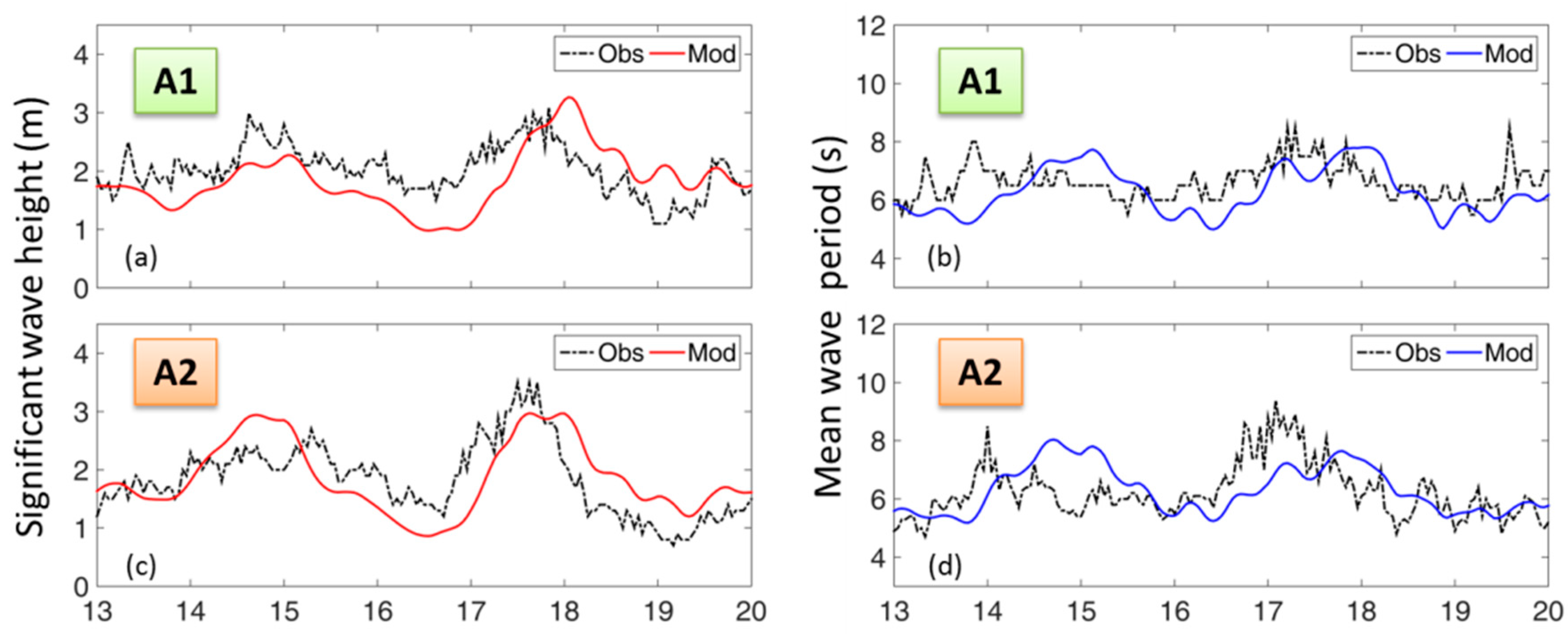
A1	121.91°E	28.44°N	0.54	0.91	--
A2	121.10°E	27.41°N	0.53	1.00	--
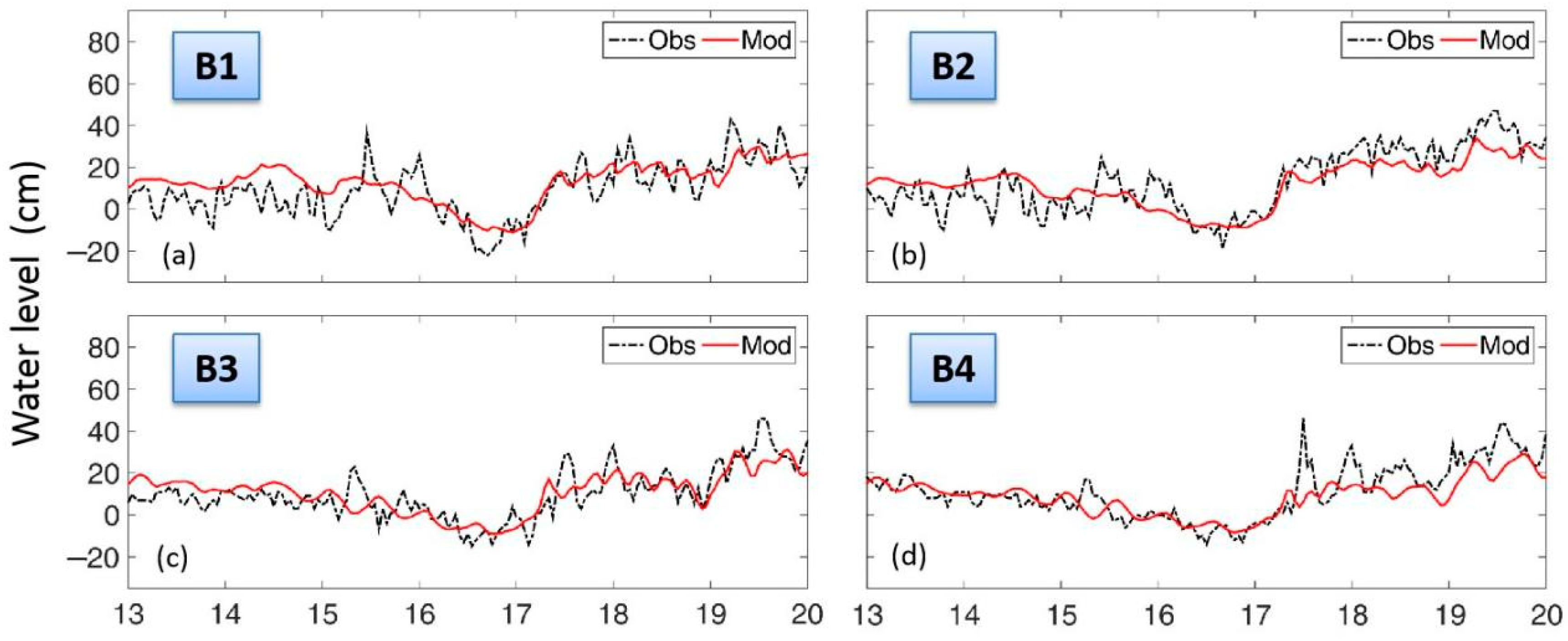
B1	121.61°E	30.61°N	--	--	9.58
B2	121.73°E	29.98°N	--	--	8.92
B3	121.96°E	29.21°N	--	--	7.77
B4	121.90°E	28.45°N	--	--	8.10

. The root mean square error (RMSE) of the significant wave height (SWH) is about 0.54 m. The RMSE of the wave period is about 1 s. The RMSE of the water level is less than 10 cm. The overall modeled wave and water level matches well with the measurements.

Time series of wave parameters of observations and model outputs are given in Figure 4. The horizontal axis coordinate represents the period from 13 September to 20 September 2016. The SWH varies between 1 m and 4 m, and the mean wave period ranges from 5 s to 9 s. There are two crests during the period, and the model results have a consistent tendency to match with the observations.

Time series of the water levels of the observations and model outputs are presented in Figure 5. The horizontal axis coordinate represents the period from 13 September to 20 September 2016. The water level fluctuates between −20 cm and 40 cm. There is a trough during 16–17 September 2016. The tendencies observed in the simulation and observation are in agreement.

The comparison between the results of the observation and the model indicates that the model results reproduced in situ observations well. The impact of Typhoon Malakas on the area around the Zhoushan Islands was remarkable during 17–18 September 2016. The model results of the storm tidal current field and ocean surface waves at 12:00 on 17 September 2016 are given in Figure 6.

3. Results

An analytic model, proposed in Section 2.1, considers wave–current–bottom interaction and is capable of estimating the variation of the orbital motion of waves near the sea floor. Ocean data regarding model outputs mentioned in Section 2.2 reproduce the observations well. In this section, based on the ocean data, we aim to roughly estimate the magnitude of the variation of amplitude of wave orbital velocity using the analytic model. This estimation contributes to understanding of the wave–current–bottom interaction in coastal areas and may be helpful in improving wave models. The results of theoretical analysis for an ideal island are given in Section 3.1. The results of practical application in the Shengsi area are presented in Section 3.2.

3.1. Results of Theoretical Analysis

We assume that there is an ideal island with a large gradient of bottom topography in the ocean, as shown in Figure 7. Water depth increases with the increasing distance away from the central island. Therefore, for an arbitrary point in the northwest of the island, e.g., P₁, water depth, H, increases gradually along the positive direction of the x₁ axis and the gradient of bottom topography $\frac{\partial H}{\partial x_1}<0$ at P₁. Similarly, water depth, H, decreases along the positive direction of the x₂ axis and the gradient of bottom topography $\frac{\partial H}{\partial x_2}>0$ at P₁. The bottom slope for the ideal island is shown in different directions in Figure 7.

Four points in different directions {P₁, P₂, P₃, and P₄} represent four classic types of bottom slope. Here, we assume that the absolute values of bottom slope gradient for these four points are all 0.5. Specific values are listed in

Table 4. Bottom slope of points {P₁, P₂, P₃, P₄}.

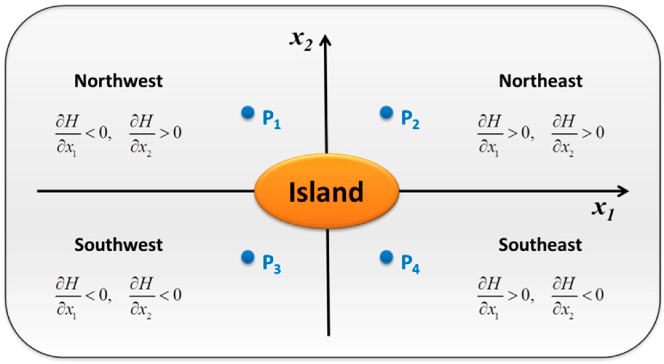
Bottom Slope	P1	P2	P3	P4
$\partial H/\partial x_1$	−0.5	0.5	−0.5	0.5
$\partial H/\partial x_2$	0.5	0.5	−0.5	−0.5

. Subsequently, we assume that the ocean states of points {P₁, P₂, P₃, and P₄} are consistent with those of location (122°50′E, 30°41′N) at 12:00 on 17 September 2016 as shown in Figure 6.

Current and wave can be decomposed into current components {CurC₁, CurC₂, ..., CurC_n, ...} and wave components {WavC₁, WavC₂, ..., WavC_n, ...}, respectively, via Fourier transformation. CurC_n and WavC_n have the same wave number, k_n, and absolute radian frequency, ${\omega }_{\mathrm{n}}$, in the phase space. If the amplitude, ${\mu }_{\left(U_2\right)}$, of CurC_n is not equal to zero, there is a resonance between CurC_n and WavC_n.

With respect to points {P₁, P₂, P₃, P₄}, the variation of the wave orbital motion for the main characteristic wave component, WavC_main, and overall variation for all wave components are estimated in Section 3.1.1 and Section 3.1.2, respectively.

3.1.1. Analysis for Main Characteristic Wave Component

According to the analytic model (Equations (19)–(23)) we proposed, variables related to current, wave, and bottom topography, e.g., the gradient of vertical current velocity, $\frac{\partial U_2}{\partial x_3}$, the amplitude of each current component, ${\mu }_{\left(U_2\right)}$, the wave number, k, and the absolute radian frequency, $\omega$, of the main characteristic wave component, water depth, H, and bottom slope ($\frac{\partial H}{\partial x_1}$ and $\frac{\partial H}{\partial x_2}$), are necessary to calculate the variation of wave orbital velocity.

First, the original current field at 12:00 on 17 September 2016 with a spatial resolution of 1/350° × 1/350° is interpolated into grids of 10 m × 10 m. Then, we decompose current velocity in the x₂ direction at points {P₁, P₂, P₃, P₄}, i.e., location (122°50′E, 30°41′N), using the FFT function in MATLAB. Thus, the amplitude of each current component, ${\mu }_{\left(U_2\right)}$, is obtained. Finally, the wave number, k, and the absolute radian frequency, $\omega$, of the main characteristic wave component are calculated using the dispersion relationship, wave mean period, and wave mean direction. The water depth, H = 34.4 m. Here, we set $\frac{\partial U_2}{\partial x_3}=0.2$ s⁻¹.

The variation of amplitude of the orbital motion for the main characteristic wave component, WavC_main, is shown in Figure 8. As we assume that ocean states, i.e., current and wave, are the same at points {P₁, P₂, P₃, P₄}, bottom slope is the only variable factor. Horizontal and vertical variations gradually decrease with the decreasing water depth. This indicates that wave–current resonance that occurs near the sea floor has more significant effect on near-bottom particles.

At the bottom, i.e., $x_3=-H$, $\left|\Delta {\mu }_3\right|$ is larger than 3 m³/s. In the north of the central island, $\Delta {\mu }_3<0$, while in the south $\Delta {\mu }_3>0$. According to the analytic model in Section 2.1, $\Delta {\mu }_3$ is dominantly related to the product of bottom slope $\frac{\partial H}{\partial x_2}$ and the amplitude of current component ${\left({\mu }_{\left(U_2\right)}\right)}_{x_3=-H}$. $\Delta {\mu }_3$ is only meaningful when these two factors exist concurrently. This is the reason why the effect of wave–current resonance is at its maximum at the bottom.

The absolute of horizontal variations $\Delta {\mu }_1$ and $\Delta {\mu }_2$ are both less than $\left|\Delta {\mu }_3\right|$. Wave–current–bottom interaction influences the vertical velocity of a wave more significantly than it does horizontal velocity.

Furthermore, these two horizontal variations always have an opposite plus–minus sign. This difference is determined by the wave number, k₁. If a wave propagates towards the west, i.e., k₁ < 0, horizontal variations $\Delta {\mu }_1$ and $\Delta {\mu }_2$ have an opposite plus–minus sign, while if a wave propagates to the east, i.e., k₁ > 0, plus–minus signs of horizontal variations are the same.

3.1.2. Analysis for All Wave Components

According to Equation (17), the overall variation of the orbital motion for all the wave components can be obtained through the use of the integral of $\Delta {\mu }_{\mathsf{\alpha }} (\mathsf{\alpha }=1,2,3$) over the whole wave number space. The result is shown in Figure 9. The overall variation of all wave components and variation of the main characteristic wave component has an analogous tendency.

Horizontal and vertical variations gradually decrease with the decreasing water depth. At the sea floor, i.e., $x_3=-H$, $\left|\Delta {\overline{\mu }}_{\left(u_1\right)}\right|$ is roughly 0.1 m/s; $\left|\Delta {\overline{\mu }}_{\left(u_2\right)}\right|$ is close to zero; $\left|\Delta {\overline{\mu }}_{\left(u_3\right)}\right|$ is larger than 0.4 m/s. In coastal areas, the tide current can reach up to 2 m/s [52]. Therefore, the vertical variation of the wave orbital velocity is pronounced. This is significant for physical processes, e.g., hydrodynamics and sediment transport in coastal areas.

3.2. Results of Shengsi Area

In this section, the analytic model we proposed in Section 2.1 is applied to the Shengsi area, where there are many islands surrounded by complicated bottom topography. The variation of wave orbital motion for the main characteristic wave component near Shengshan Island and Gouqi Island during the period of Typhoon Malakas is calculated in Section 3.2.1. The overall variation for all wave components is roughly estimated in Section 3.2.2.

In the theoretical analysis of an ideal island (Section 3.1), the absolute value of the bottom slope gradient is 0.5. Large gradients of bottom topography in the Shengsi area widely exist in practice conditions. There are many locations where the magnitude order of a topographical slope is 10⁻¹ in nautical charts. However, the water depth of the ocean data described in Section 2.2 with a spatial resolution of 1/350° × 1/350° is too coarse to reproduce the real gradient of bottom topography, which is shown in Figure 10. We found that a fivefold/tenfold value of the coarse bottom slope is close to the real bottom slope. Therefore, after multiplying by a coefficient 5 or 10, the coarse bottom slope was used to estimate the variation of the orbital motion of waves in the Shengsi area during Typhoon Malakas.

3.2.1. Analysis for Main Characteristic Wave Component

During the period of Typhoon Malakas, the storm tide current became stronger. The effect of this typhoon on the Shengsi area was most remarkable on 17 September 2016. Therefore, we estimated the variation of the wave orbital motion at 12:00 on 17 September 2016 using the analytic model proposed in Section 2.1 based on the ocean data described in Section 2.2. Horizontal and vertical variations of the amplitude of wave orbital motion at the sea floor for the main characteristic wave component are shown in Figure 11.

The spatial distribution of current and ocean surface waves at 12:00 on 17 September 2016 are shown in Figure 6. First, the original current field at 12:00 on 17 September 2016 with spatial resolution 1/350° × 1/350° was interpolated into grids of 10 m × 10 m. Then, we decomposed the current velocity in the x₂ direction at each point near Gouqi Island and Shengsi Island via the FFT function in MATLAB. Thus, the amplitude of each current component, ${\mu }_{\left(U_2\right)}$, for each point was obtained. Finally, the wave number, k, and absolute radian frequency, $\omega$, of the main characteristic wave component were calculated using the dispersion relationship, wave mean period and wave mean direction. Here, $\frac{\partial U_2}{\partial x_3}$ was 0.2 s⁻¹. Note that the results of fivefold bottom slope and tenfold bottom slope for values $\left\{\Delta {\mu }_1,\Delta {\mu }_2,\Delta {\mu }_3\right\}$ are shown in Figure 11a–c and Figure 11d–f, respectively.

Vertical variation, $\Delta {\mu }_3$, in Figure 11c is between (−1, 1) m³/s, while horizontal variations, $\Delta {\mu }_1$ and $\Delta {\mu }_2$, in Figure 11a,b are between (−0.05, 0.05) m³/s. The current and bottom slope influence the vertical orbital motions of a wave than they do the horizontal orbital motions of wave.

The colors in the figures represent whether the amplitude of the wave orbital motion for the main characteristic wave component increases (red) or decreases (blue). There are enhanced or weakened effects of the current and bottom slope on the wave orbital motion. Variations $\Delta {\mu }_1$ and $\Delta {\mu }_2$ always have an opposite plus–minus sign at the same position. At most points, vertical variation, $\Delta {\mu }_3$, is larger than zero, i.e., the amplitude of the wave orbital motion is enhanced due to the current and bottom slope.

Furthermore, comparison between Figure 11a–c and Figure 11d–f indicates that variations of the wave orbital motion are more pronounced if the bottom slope gradient is larger.

3.2.2. Analysis for All Wave Components

The overall variations of the amplitude of wave orbital motion at the sea floor for all wave components at 12:00 on 17 September 2016 are estimated using the analytic model proposed in Section 2.1 based on the ocean data described in Section 2.2. The results of the fivefold bottom slope and tenfold bottom slope for $\left\{\Delta {\overline{\mu }}_1,\Delta {\overline{\mu }}_2,\Delta {\overline{\mu }}_3\right\}$ are shown in Figure 12a–c and Figure 12d–f, respectively.

The spatial distribution of overall variations (Figure 12) and variations for the main characteristic wave component (Figure 11) is similar. Variations $\Delta {\overline{\mu }}_1$ and $\Delta {\overline{\mu }}_2$ always have an opposite plus–minus sign at the same position. At most points, vertical variation, $\Delta {\overline{\mu }}_3$, is larger than zero, i.e., the amplitude of wave orbital motion is enhanced due to the current and bottom slope.

In Figure 12c, vertical variation, $\Delta {\overline{\mu }}_3$, is shown to be between (−0.5, 0.5) m/s, which is close to the velocity of the tide current in coastal areas [52], while in Figure 12a,b, horizontal variations, $\Delta {\overline{\mu }}_1$ and $\Delta {\overline{\mu }}_2$, are between (−0.01, 0.01) m/s. Therefore, the variation of the vertical orbital velocity of a wave is pronounced. This is significant for physical processes, e.g., hydrodynamics and sediment transport in coastal areas.

Comparison between Figure 12a–c and Figure 12d–f indicates that variations of wave orbital motion are more pronounced if the bottom slope gradient is larger.

4. Discussion

Wave–current interaction plays an important role in coastal areas and has a significant impact on coastal dynamics, storm surges, and sediment transport. In extreme weather conditions, this issue is even more significant.

Some theories related to wave–current interaction, e.g., radiation stress and wave action conservation, have been established and applied in numerical simulation models. Most wave models, e.g., SWAN, consider the bottom friction source term. However, the bottom slope value, which might have a significant effect on a wave, has been ignored.

In this study, based on a unified linear theory of wavelike perturbations [41], we proposed an analytic model which is capable of estimating the variation of amplitude of wave orbital motion due to current and bottom slope. Subsequently, variations for main characteristic wave components and all wave components were roughly calculated based on the ocean data obtained during Typhoon Malakas.

First this analytic model was applied on an ideal island. The characteristics of the gradient of bottom topography are presented. The results indicate that wave–current resonance that occurs near the sea floor has a more significant effect on near-bottom particles, as horizontal and vertical variations gradually decrease with the decreasing water depth. At the sea floor, i.e., $x_3=-H$, the absolute value of vertical variation of amplitude of wave orbital motion for the main characteristic wave component $\left|\Delta {\mu }_3\right|$ is larger than 3 m³/s; the absolute value of overall variation of amplitude of wave orbital motion in the vertical direction $\left|\Delta {\overline{\mu }}_{\left(u_3\right)}\right|$ is larger than 0.4 m/s.

Next, the analytic model was applied in the Shengsi area, which lies in the center of the famous Zhoushan Fishing Ground. Bottom topography is complicated in this region. At the sea floor, the vertical variation of the amplitude of wave orbital motion for the main characteristic wave component $\left|\Delta {\mu }_3\right|$ is between (−1, 1) m³/s; the absolute value of overall variation of the amplitude of wave orbital motion in the vertical direction $\left|\Delta {\overline{\mu }}_{\left(u_3\right)}\right|$ is between (−0.5, 0.5) m/s. In coastal areas, the tide current can reach up to 2 m/s [45]. Therefore, the vertical variation of wave orbital velocity is pronounced. This is significant for physical processes, e.g., hydrodynamics and sediment transport in coastal areas.

This paper is a preliminary study with respect to the effect of current and bottom slope values on waves, e.g., the velocity of mean flow is $\left\{0,U_2\left(x_1,x_2,x_3\right),0\right\}$. This simplification will be abandoned in further research. Furthermore, observations regarding wave orbital motion will be used to validate and evaluate the accuracy of the analytic model in the future. Ultimately, the parameterization term related to the effect of the current and bottom slope on a wave is planned to construct in a wave equation.

5. Conclusions

The coast of China possesses complex topography. The coupling effect between a strong current and ocean waves is very strong during storm surges, especially in a situation where the topographic gradient is large. However, its physical mechanism is still not understood. Based on the unified linear wave theory, this study analyzed the effect of strong currents and bottom slope values on the orbital velocity amplitude of ocean waves in dynamics and established a corresponding analytic model. Based on this analytic model, theoretical analysis and an implemented example in the Shengsi area during Typhoon Malakas are given. The results suggest that the impact of wave–current interaction is noticeable where the sea bottom slope gradient is relatively large. This study is helpful in improving the numerical simulation of ocean waves.

References

- Tolman, H.L. A third-generation model for wind-waves on slowly varying, unsteady, and inhomogeneous depths and currents. J. Phys. Oceanogr. 1991, 21, 782–797. [Google Scholar] [CrossRef]
- Yuan, Y.L.; Qiao, F.L.; Yin, X.Q.; Han, L.; Lu, M. Establishment of the ocean dynamic system with four sub-systems and the derivation of their governing equation sets. J. Hydrodyn. 2012, 24, 153–168. [Google Scholar] [CrossRef]
- Viitak, M.; Maljutenko, I.; Alari, V.; Suursaar, Ü.; Rikka, S.; Lagemaa, P. The impact of surface currents and sea level on the wave field evolution during St. Jude storm in the eastern Baltic Sea. Oceanologia 2016, 58, 176–186. [Google Scholar] [CrossRef] [Green Version]
- Prakash, K.R.; Pant, V. On the wave-current interaction during the passage of a tropical cyclone in the bay of bengal. Deep Sea Res. Part II Top. Stud. Oceanogr. 2019, 172, 104658. [Google Scholar] [CrossRef]
- Song, H.L.; Kuang, C.P.; Wang, X.H.; Ma, Z. Wave-current interactions during extreme weather conditions in southwest of Bohai Bay, China. Ocean Eng. 2020, 216, 108068. [Google Scholar] [CrossRef]
- Cavaleri, L.; Fox-Kemper, B.; Hemer, M. Wind waves in the coupled climate system. Bull. Am. Meteorol. Soc. 2012, 93, 1651–1661. [Google Scholar] [CrossRef]
- Unna, P.J. White horses. Nature 1941, 148, 226–227. [Google Scholar] [CrossRef]
- Unna, P.J. Waves and tidal streams. Nature 1942, 149, 219–220. [Google Scholar] [CrossRef]
- Unna, P.J. Sea waves. Nature 1947, 159, 239–242. [Google Scholar] [CrossRef]
- Barber, N.F. The behaviour of waves on tidal streams. Proc. R. Soc. Lond. Ser. A Math. Phys. Sci. 1949, 198, 81–93. [Google Scholar] [CrossRef] [Green Version]
- Longuet-Higgins, M.S.; Stewart, R.W. Changes in the form of short gravity waves on long waves and tidal currents. J. Fluid Mech. 1960, 8, 565. [Google Scholar] [CrossRef]
- Longuet-Higgins, M.S.; Stewart, R.W. The changes in amplitude of short gravity waves on steady non-uniform currents. J. Fluid Mech. 1961, 10, 529. [Google Scholar] [CrossRef]
- Longuet-Higgins, M.S.; Stewart, R.W. Radiation stress and mass transport in gravity waves, with application to ‘surf beats’. J. Fluid Mech. 1962, 13, 481. [Google Scholar] [CrossRef]
- Longuet-Higgins, M.S.; Stewart, R.W. Radiation stresses in water waves—A physical discussion, with applications. Deep Sea Res. 1964, 11, 529–562. [Google Scholar] [CrossRef]
- Whitham, G.B. A general approach to linear and non-linear dispersive waves using a Lagrangian. J. Fluid Mech. 1965, 22, 273. [Google Scholar] [CrossRef]
- Bretherton, F.P.; Garrett, C. Wavetrains in inhomogeneous moving media. Proc. R. Soc. Lond. Ser. A Math. Phys. Sci. 1968, 302, 529–554. [Google Scholar] [CrossRef]
- Whitham, G.B. Linear and Nonlinear Waves; Wiley: New York, NY, USA, 1974. [Google Scholar]
- Phillips, O.M. The Dynamics of the Upper Ocean, 2nd ed.; Cambridge University Press: Cambridge, UK, 1977. [Google Scholar]
- Mei, C.C. The Applied Dynamics of Ocean Surface Waves; Wiley: New York, NY, USA, 1983. [Google Scholar]
- Dingemans, M.W. Water Wave Propagation Over Uneven Bottoms; World Scientific: London, UK, 1997. [Google Scholar]
- Mellor, G.L. The three-dimensional current and surface wave equations. J. Phys. Oceanogr. 2003, 33, 1978–1989. [Google Scholar] [CrossRef]
- Mellor, G.L. The depth-dependent current and wave interaction equations: A revision. J. Phys. Oceanogr. 2008, 38, 2587–2596. [Google Scholar] [CrossRef]
- Mellor, G.L. A combined derivation of the integrated and vertically resolved, coupled wave-current equations. J. Phys. Oceanogr. 2015, 45, 1453–1463. [Google Scholar] [CrossRef]
- Ji, C.; Zhang, Q.H.; Wu, Y.S. Derivation of three-dimensional radiation stress based on Lagrangian solutions of progressive waves. J. Phys. Oceanogr. 2017, 47, 2829–2842. [Google Scholar] [CrossRef]
- McWilliams, J.C.; Restrepo, J.M. The wave-driven ocean circulation. J. Phys. Oceanogr. 1999, 29, 2523–2540. [Google Scholar] [CrossRef]
- Uchiyama, Y.; McWilliams, J.C.; Shchepetkin, A.F. Wave-current interaction in an oceanic circulation model with a vortex-force formalism: Application to the surf zone. Ocean Model. 2010, 34, 16–35. [Google Scholar] [CrossRef]
- Bennis, A.C.; Ardhuin, F.; Dumas, F. On the coupling of wave and three-dimensional circulation models: Choice of theoretical framework, practical implementation and adiabatic tests. Ocean Model. 2011, 40, 260–272. [Google Scholar] [CrossRef] [Green Version]
- Kumar, N.; Voulgaris, G.; Warner, J.C.; Olabarrieta, M. Implementation of the vortex force formalism in the coupled ocean-atmosphere-wave-sediment transport (COAWST) modeling system for inner shelf and surf zone applications. Ocean Model. 2012, 47, 65–95. [Google Scholar] [CrossRef]
- Yuan, Y.L.; Qiao, F.L.; Hua, F.; Wan, Z. The development of a coastal circulation numerical model: Ⅰ. Wave-induced mixing and wave-current interaction. J. Hydrodyn. Ser. A 1999, 14, 1–8. [Google Scholar]
- Yang, Y.Z.; Qiao, F.L.; Xia, C.S.; Ma, J.; Yuan, Y.L. Wave-induced mixing in the Yellow Sea. Chin. J. Oceanol. Limnol. 2004, 22, 322–326. [Google Scholar] [CrossRef]
- Qiao, F.L.; Yuan, Y.L.; Yang, Y.Z.; Zheng, Q.A.; Xia, C.S.; Ma, J. Wave-induced mixing in the upper ocean: Distribution and application to a global ocean circulation model. Geophys. Res. Lett. 2004, 31, L11303. [Google Scholar] [CrossRef]
- Deltares. SWAN Scientific and Technical Documentation; Deltares: Delft, The Netherlands, 2021. [Google Scholar]
- Günther, H.; Hasselmann, S.; Janssen, P.A.E.M. The WAM Model Cycle 4; Deutsches Klimarechenzentrum (DKRZ): Hamburg, Germany, 1992. [Google Scholar]
- Booij, N.; Ris, R.C.; Holthuijsen, L.H. A third-generation wave model for coastal regions: 1. Model description and validation. J. Geophys. Res. Ocean. 1999, 104, 7649–7666. [Google Scholar] [CrossRef] [Green Version]
- Yuan, Y.L.; Pan, Z.D.; Hua, F.; Sun, L.T. LAGFD-WAM wave numerical model (I), the basic physical model. Acta Oceanol. Sin. 1992, 14, 1–7. [Google Scholar]
- Yuan, Y.L.; Hua, F.; Pan, Z.D.; Sun, L.T. LAGFD-WAM numerical wave model-II. Characteristics inlaid scheme and its application. Acta Oceanol. Sin. 1992, 14, 12–24. [Google Scholar]
- Yang, Y.L.; Qiao, F.L.; Zhao, W.; Teng, Y.; Yuan, Y.L. MASNUM ocean wave numerical model in spherical coordinates and its application. Acta Oceanol. Sin. 2005, 27, 1–7. [Google Scholar] [CrossRef]
- Shemdin, P.; Hasselmann, K.; Hsiao, S.V.; Herterich, K. Non-linear and linear bottom interaction effects in shallow water. In Turbulent Fluxes through the Sea Surface, Wave Dynamics, and Prediction; Springer: Boston, MA, USA, 1978; Volume 1, pp. 347–372. [Google Scholar] [CrossRef]
- Bertotti, L.; Cavaleri, L. Accuracy of wind and wave evaluation in coastal regions. In Proceedings of the 24th International Conference on Coastal Engineering, Kobe, Japan, 23–28 October 1994. [Google Scholar] [CrossRef]
- Gorrell, L.; Raubenheimer, B.; Elgar, S.; Guza, R.T. SWAN predictions of waves observed in shallow water onshore of complex bathymetry. Coast. Eng. 2011, 58, 510–516. [Google Scholar] [CrossRef]
- Yuan, Y.L.; Han, L.; Qiao, F.L.; Yang, Y.Z.; Lu, M. A unified linear theory of wavelike perturbations under general ocean conditions. Dyn. Atmos. Oceans 2011, 51, 55–74. [Google Scholar] [CrossRef]
- Chen, X.G.; Wang, J.L.; Cukrov, N.; Du, J.Z. Porewater-derived nutrient fluxes in a coastal aquifer (Shengsi Island, China) and its implication. Estuar. Coast. Shelf Sci. 2019, 218, 204–211. [Google Scholar] [CrossRef]
- ADCIRC. Available online: https://adcirc.org/ (accessed on 17 July 2020).
- Feng, X.R.; Li, M.J.; Yin, B.S.; Yang, D.Z.; Yang, H.M. Study of storm surge trends in typhoon-prone coastal areas based on observations and surge-wave coupled simulations. Int. J. Appl. Earth Obs. Geoinf. 2018, 68, 272–278. [Google Scholar] [CrossRef]
- Li, T.; Wang, F.D.; Hou, J.M.; Che, Z.M.; Dong, J.X. Validation of an operational forecasting system of sea dike risk in the southern Zhejiang Province, South China. J. Oceanol. Limnol. 2019, 37, 1929–1940. [Google Scholar] [CrossRef]
- Wang, Y.P.; Liu, Y.L.; Mao, X.Y.; Chi, Y.T.; Jiang, W.S. Long-term variation of storm surge-associated waves in the Bohai Sea. J. Oceanol. Limnol. 2019, 37, 1868–1878. [Google Scholar] [CrossRef]
- Yang, W.K.; Feng, X.R.; Yin, B.S. The impact of coastal reclamation on tidal and storm surge level in Sanmen Bay, China. J. Oceanol. Limnol. 2019, 37, 1971–1982. [Google Scholar] [CrossRef]
- Zhang, W.S.; Teng, L.; Zhang, J.S.; Xiong, M.J.; Yin, C.T. Numerical study on eff ect of tidal phase on storm surge in the South Yellow Sea. J. Oceanol. Limnol. 2019, 37, 2037–2055. [Google Scholar] [CrossRef]
- Cavaleri, L.; Malanotte-Rizzoli, P. Wind wave prediction in shallow water: Theory and applications. J. Geophys. Res. 1981, 86, 10961–10973. [Google Scholar] [CrossRef]
- Janssen, P.A.E.M. Quasi-linear theory of wind-wave generation applied to wave forecasting. J. Phys. Oceanogr. 1991, 21, 1631–1642. [Google Scholar] [CrossRef] [Green Version]
- Weather China. Available online: http://www.weather.com.cn/ (accessed on 17 July 2020).
- Sun, X.P. China Offshore Regional Oceans; Ocean Press: Beijing, China, 2006. [Google Scholar]