GAN-GL: Generative Adversarial Networks for Glacial Lake Mapping

Abstract

Remote sensing is a powerful tool that provides flexibility and scalability for monitoring and investigating glacial lakes in High Mountain Asia (HMA). However, existing methods for mapping glacial lakes are designed based on a combination of several spectral features and ancillary data (such as the digital elevation model, DEM) to highlight the lake extent and suppress background information. These methods, however, suffer from either the inevitable requirement of post-processing work or the high costs of additional data acquisition. Signifying a key advancement in the deep learning models, a generative adversarial network (GAN) can capture multi-level features and learn the mapping rules in source and target domains using a minimax game between a generator and discriminator. This provides a new and feasible way to conduct large-scale glacial lake mapping. In this work, a complete glacial lake dataset was first created, containing approximately 4600 patches of Landsat-8 OLI images edited in three ways—random cropping, density cropping, and uniform cropping. Then, a GAN model for glacial lake mapping (GAN-GL) was constructed. The GAN-GL consists of two parts—a generator that incorporates a water attention module and an image segmentation module to produce the glacial lake masks, and a discriminator which employs the ResNet-152 backbone to ascertain whether a given pixel belonged to a glacial lake. The model was evaluated using the created glacial lake dataset, delivering a good performance, with an F1 score of 92.17% and IoU of 86.34%. Moreover, compared to the mapping results derived from the global–local iterative segmentation algorithm and random forest for the entire Eastern Himalayas, our proposed model was superior regarding the segmentation of glacial lakes under complex and diverse environmental conditions, in terms of accuracy (precision = 93.19%) and segmentation efficiency. Our model was also very good at detecting small glacial lakes without assistance from ancillary data or human intervention.

1. Introduction

During the last several decades, glacial lakes have increased dramatically in area and number in High Mountain Asia (HMA) due to the ongoing impact of global warming and glacier melting [1]. This has considerably increased the risk of flood outburst hazards and, therefore, monitoring and evaluating the dynamics of glacial lakes is of great significance for the understanding of ecosystem stability and preventing outburst hazards in downstream areas. Fast and accurate mapping of glacial lakes is a prerequisite for the comprehensive investigation of these lakes.

As a unique water resource, glacial lakes have several remarkable characteristics. (1) Small size: small glacial lakes (<0.1 km²) make up the majority of the glacial lakes in HMA. For example, more than 72.7% of the glacial lakes were small in size in 2016 [2,3]. Although these small lakes pose a limited threat to downstream regions, they are still a key factor in exhibiting the dynamic of climate change and giving larger uncertainties in glacial lake mapping [4]. (2) Various physical properties: affected by environmental components such as soil, geology, vegetation, and glaciers, glacial lakes show varying degrees of turbidity and coloring in remote sensing imagery. Moreover, some objects, such as mountain shadows and clouds [1], have a spectrum similar to that of glacial lakes. Thus, the spectral characteristics of glacial lakes vary in complexity with diverse environmental conditions. (3) Wide distribution: glacial lakes of different types, sizes, and shapes are widely distributed around glaciers in the alpine regions of Central and South Asia [5], including the Altai Mountains [6], Himalayas [7,8], Tianshan Mountains [9], and Kunlun Mountains [10], as well as the Karakoram-Pamir Plateau [11,12]. All of these unique characteristics provide great challenges for the automatic and accurate mapping of glacial lakes over a very large-scale glaciated area.

Although much progress has been made in mapping glacial lakes, the mapping methods involved require significant post-processing work and the use of other ancillary data, such as the digital elevation model (DEM) and feature maps. One fundamental problem in glacial lake mapping is that all the features used to highlight glacial lake information are manually designed. This means that while certain spectral or handcrafted features are used, other useful high-level and complex features are ignored. For instance, water indexes [13] are the most commonly used spectral features for the detection of glacial lakes, and they are designed as band ratios that involve green/blue (G/B) bands and near-infrared/short wave infrared (NIR/SWIR) bands. However, many phenomena (such as mountain shadows, melting glaciers, and clouds) generate spectral responses similar to those of glacial lakes, resulting in low mapping accuracy and inevitable manual correction. To alleviate the effects of these factors, most semi-automatic methods use auxiliary data to minimize the amount of less post-processing required. Song et al. [4] presented a hierarchical image segmentation method to explore the distribution and evolution of glacial lakes in the Southeastern Tibetan Plateau. The method combined the normalized difference water index (NDWI) derived from Landsat TM/ETM+/OLI imagery with DEM-based terrain analysis results to extract glacial lake areas. Li et al. [14] proposed a global–local iterative segmentation algorithm to delineate glacial lake extent using Landsat TM/ETM+ and DEM data. Shen et al. [15] applied an object-oriented classification method to extract glacial lake information using a water extraction decision ruleset. This method, however, requires many experiments to determine which features should be considered and how to set parameter values, such as the segmentation scale, shape index, and NDWI. Bhardwaj et al. [16] designed a lake detection algorithm (LDA), which comprised inputs from the moisture index, vegetation index, and NDWI to detect lake pixels and filter out noise pixels based on the DEM and thermal information. Gao et al. [17] established a lake hydrological network to identify the attributes of each lake in the Third Pole using Landsat images, topographic maps, and DEM data. Wangchuk et al. [1] employed a random forest classifier to map glacial lakes using multi-source optical and radar data, including Sentinel-1 synthetic aperture radar, Sentinel-2 multispectral instrument, and DEM. Zhao et al. [18] integrated the advantages of the threshold segmentation method and the active contour model to improve the efficient extraction of glacial lakes and the removal of mountain shadows with the help of DEM. Li et al. [19] created a two-stage segmentation workflow for mapping glacial lakes. First, the object-oriented method was used to segment the target image into the lake, potential lake, and unknown region. Then the potential lake zone was refined using the watershed algorithm. All of these methods depend on auxiliary data to some extent, and checking and editing the mapping results requires great effort. This significantly limits the use of the mapping methods for the fast and accurate extraction of large-scale glacial lake distribution information. Developing a more automatic and less data-dependent method for mapping glacial lakes suitable for large, glaciated regions, is clearly essential to explore the relationship between the changes from climate and glacial lakes, and give forewarning of the glacial lakes that have high outburst risk.

With the explosive growth in remote sensing imaging data, many effective data processing methods have been proposed. Among these, deep learning models have attracted considerable attention and shown great potential in the extraction of high-level information of objects in terms of classification [20], segmentation [21], and generation [22]. To date, there has been scant research that uses deep learning models for glacial lake mapping. Qayyum et al. [23] attempted to map glacial lakes using four-band PlanetScope imagery of the Hindu Kush, Karakoram, and Himalaya (HKKH) region using U-Net architecture. Wu et al. [24] employed a U-Net-based model to extract the contours of glacial lakes in Southeastern Tibet, with the input from Landsat-8 OLI and Sentinal-1A SAR images. Although the pooling operations in the U-Net model can reduce the number of model parameters without changing the image features, they omit some details of the lake boundaries. This is not conducive to the extraction of complex-shaped and small glacial lakes. Considering that the Landsat series of satellites provides the most extensive and longest records for glacial lake mapping, this paper proposes a new solution for glacial lake extraction. We used a deep learning model and Landsat images to facilitate the development of a glacial lake inventory and disaster management in HMA.

As an artistic designation in the deep learning model, the generative adversarial network (GAN) has achieved much in image generation [22], classification [25], object detection [26], image super-resolution [27], and image deblurring [28]. GAN is rarely used as a domain transfer task for image segmentation. Compared to other segmentation models, GAN defines a generator and discriminator to learn the distribution of real data and generates segmentation masks without distribution assumptions [29]. Using GAN, Xue et al. [30] proposed a SegAN model, which uses a fully convolutional neural construction in the generator to segment the mask of a brain tumor in an MRI image at the pixel level. Their model had better precision and sensitivity than other state-of-the-art models when testing it against the BRATS 2013 and 2015 datasets. Son et al. [31] used a GAN-based model to precisely map a vessel in a retinal image and obtained good results on the DRIVE and STARE datasets. To improve mapping accuracy and avoid human-interactive processing, in this paper, we propose a novel end-to-end GAN-based architecture for glacial lake mapping (GAN-GL), in which the only input data are remote sensing images. The water attention module and image segmentation module are cascaded in the generator of GAN-GL to focus on lake information. A ResNet backbone is used in the discriminator. To the best of our knowledge, this is the first time that water attention has been used in a deep learning method for glacial lake mapping. Moreover, we built a large-scale glacial lake dataset for the training and evaluation of the performance of GAN-GL. This dataset contains about 4600 Landsat image patches, each cropped around the glacial lake and with 256 × 256 × 7 pixels. We further divided the dataset into three subsets according to the collection methods, including random cropping, uniform cropping, and density cropping. This model greatly improves the segmentation of glacial lakes over a large-scale area with low data dependence. The robustness and relative accuracy of the proposed method was also tested under different environmental conditions using a global–local iterative segmentation algorithm and random forest classification as a benchmark.

The rest of this paper is organized as follows. Section 2 introduces the collection and statistical analysis of the dataset. In Section 3, we describe the methodology and the architecture of the proposed GAN-GL model. The evaluation metrics and experimental results are given in Section 4. The factors that may influence the mapping performance are discussed in Section 5. Finally, we conclude this work in Section 6.

2. Dataset

While many achievements and publications have been conducted on the glacial lake inventory [5,10], the inventory data cannot be directly used as training samples for deep learning models due to inconsistent data properties between inventory data and glacial lakes in images. In addition, format transformation and region cropping are needed to comply with the input form of the GAN network. In this section, we describe the details of the collection and production of a complete glacial lake dataset. Such a dataset can be used to drive deep learning models for automatic glacial lake mapping as well as to evaluate the performance of the deep learning model.

2.1. Collection of Dataset

Owing to its moderate spatial resolution (30 m) and continuous record, Landsat imagery has become one of the most extensively used data resources to retrieve glacial lake information. In this study, Landsat-8 OLI imagery was employed as basic data to create the GAN-GL dataset, as shown in

Table 1. Details of Landsat-8 OLI images used in this study.

Path/Row	Cloud Cover (%)	Acquisition Data	Sub-Region	Lake Number in the Tile
133/039	0.17	2 November 2016	Hengduan Shan	97
150/033	1.35	20 July 2016	E. Pamir	9
146/029	1.54	25 August 2016	E. Tianshan	32
146/030	1.66	9 August 2016	C. Tianshan	62
140/039	0.18	3 November 2016	Gangdise Shan	21
145/038	0.34	21 October 2016	Gangdise Shan	68
146/038	0.92	28 October 2016	W. Himalaya	36
149/030	0.68	15 September 2016	W. Tianshan	53
142/030	1.01	30 September 2016	E. Tianshan	27
131/039	1.38	3 October 2016	Hengduan Shan	36
133/040	1.56	2 November 2016	Hengduan Shan, Nyainqentanglha	388
143/039	1.80	23 October 2016	C. Himalaya, Gangdise Shan	308
148/029	0.88	24 September 2016	Alataw Shan	197
144/039	2.34	14 October 2016	C. Himalaya	154
150/034	3.36	20 July 2016	W. Pamir	31
147/030	1.01	10 September 2016	C. Tianshan	44
139/040	0.72	27 October 2016	Gangdise Shan	16
138/040	3.40	20 October 2016	Nyainqentanglha, E. Himalaya	253
140/040	1.66	20 October 2016	C. Himalaya, Gangdise Shan	207
137/040	1.07	29 October 2016	Nyainqentanglha, E. Himalaya	133
131/037	0.01	15 July 2016	Hengduan Shan	24
135/034	2.95	15 October 2016	Qilian	17
142/040	1.58	1 November 2016	C. Himalaya	114
131/040	1.45	4 November 2016	Hengduan Shan	61
143/030	0.75	4 August 2016	E. Tianshan	8
144/038	0.50	30 October 2016	Gangdise Shan	141
137/041	2.59	29 October 2016	E. Himalaya	240
145/039	1.40	6 November 2016	C. Himalaya	24

Note: E.: East; W.: West; C.: Central.

. To minimize the interference from seasonal snow/ice cover and clouds in glacial lake detection, the acquisition times of the images were all between July and early November. During this period, the boundaries of glacial lakes are very clear and stable because of the balanced state of glacier mass gains and losses [32,33]. The High Mountain Asia Glacial Lake Inventory (Hi-MAG) database [10], which mapped the annual glacial lake coverage from 2008 to 2017 at a 30 m resolution using Landsat series satellite imagery, was used to assist in the creation of ground truth labels for each element (glacial lake or non-glacial lake).

2.2. Production of the GAN-GL Dataset

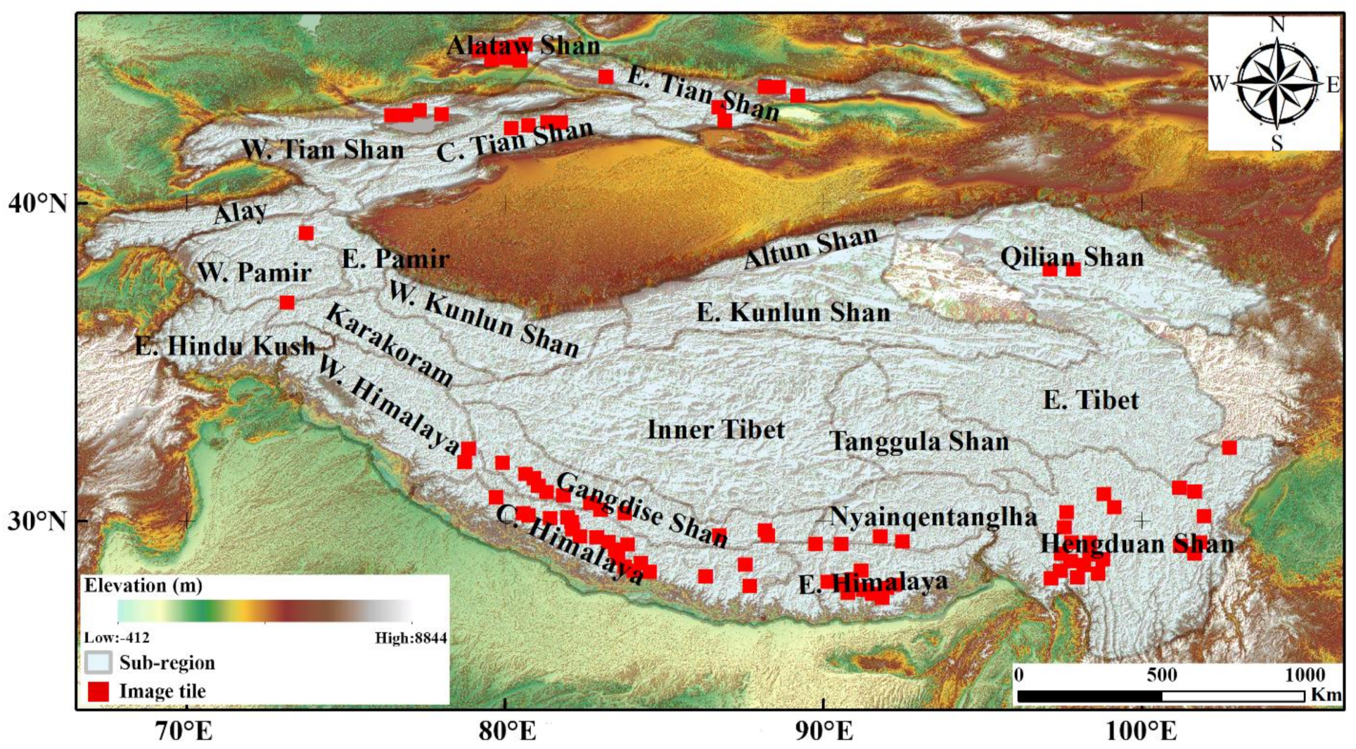
Glacial lakes are generally gathered around glaciers, and their areas are extremely small compared to backgrounds, for example, there are considerable spatial extents of non-glacial lakes in a Landsat scene. Therefore, 103 tiles, comprising 1024 × 1024 pixels and containing glacial lakes, were firstly cropped from original Landsat-8 OLI images and used as the basis for the subsequent production of the GAN-GL dataset. The spatial distribution of these tiles is shown in Figure 1.

Glacial lakes are unevenly distributed and vary greatly in size. Many glacial lakes in HMA are too small (<0.1 km²) to be identified, but they account for a large proportion of the total lake area (in Nyainqêntanglha, the area of small glacial lakes accounts for 69.47% of the total area [10]). These small lakes are quite sensitive indicators to exhibit the trends of global climate changes and are easily overlooked in lake evolution in HMA. Moreover, the density distribution of glacial lakes has high spatial heterogeneity in the glaciated regions. The density of glacial lakes is relatively high in the ranges of Southwestern Pamir as well as in the Himalayas; few glacial lakes exist in parts of Western Pamir. All this indicates that the scale and density of glacial lakes vary significantly in the HMA region, and should, therefore, be fully considered in the production of a glacial lake dataset. In this study, three forms of image cropping—uniform cropping, density cropping, and random cropping—were used to build a complete glacial lake dataset, as shown in Figure 2. Notably, the density map-based cropping method was proposed for the first time to fully utilize the spatial and contextual information from glacial lakes and to improve the detection performance of the model.

The following are the detailed steps in the production of the three glacial lake subsets:

GAN-GL-U: Uniform cropping was used for each image tile from the original GAN-GL dataset into 16 patches, each with a 256 × 256 pixel size. This subset consists of 683 patches and each lake appears only once. Some patches without any lakes were discarded.

GAN-GL-D: We cropped 256 × 256 pixels of the patches covering the glacial lakes in each image tile, and then counted the number of glacial lakes and their pixels in each patch. Only patches with more than five lakes and a total area greater than 1% of a patch area were reserved. Finally, 1540 density-cropped patches were acquired.

GAN-GL-R: To create this subset, 50 image patches, each with a size of 256 × 256 pixels, were randomly cropped from each image tile, and only image patches containing glacial lakes were retained. In this way, this subset has a total of 2382 patches, and some glacial lakes may appear more than once.

Table 2. Properties of three glacial lake subsets.

	GAN-GL-R	GAN-GL-D	GAN-GL-U
Number of image patches	2382	1540	683
Average number of glacial lakes in each patch	3.84	9.75	3.81
Average area of glacial lakes in each patch (pixel)	329.48	1225.39	332.54
Average area of each glacial lake (pixel)	85.80	125.68	87.28

lists the statistical results associated with these three subsets. GAN-GL-R and GAN-GL-U have similar values for the average number, the average area of glacial lakes in each patch, and the size of glacial lakes. GAN-GL-D has the highest density of glacial lakes.

3. Methods

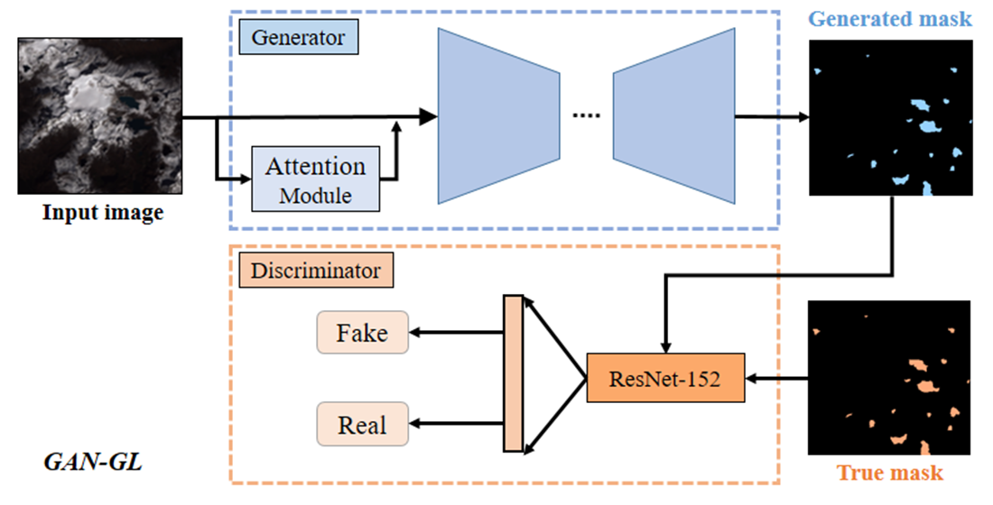
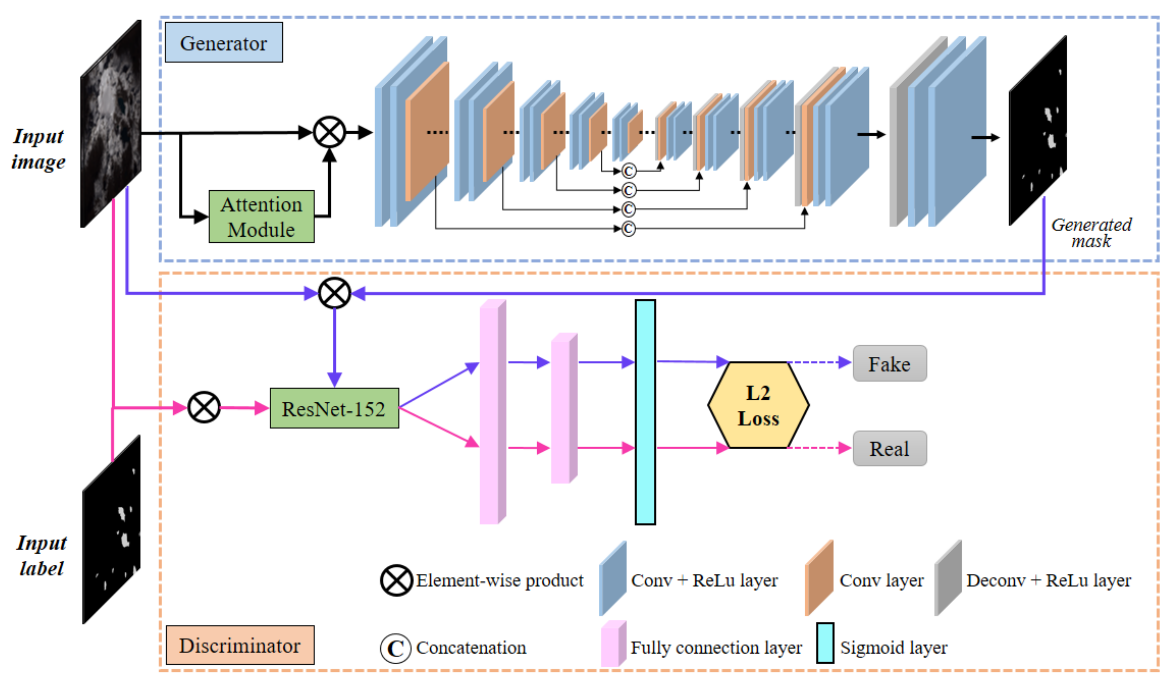
The architecture of our proposed GAN-GL model for the segmentation of glacial lakes is shown in Figure 3. In GAN-GL, we incorporated a water attention module and image segmentation module into the generator. The discriminator was designed based on ResNet-152 to encode the lake area as vectors and determine their categories. Given a remotely sensed image input, the generator attempts to produce glacial lake masks. Then, the generated masks and true labeled masks are both fed into the discriminator for training until they can correctly predict whether the input data are generated or real. In the following subsections, we describe each process in more detail.

3.1. Generator

3.1.1. Water Attention Module

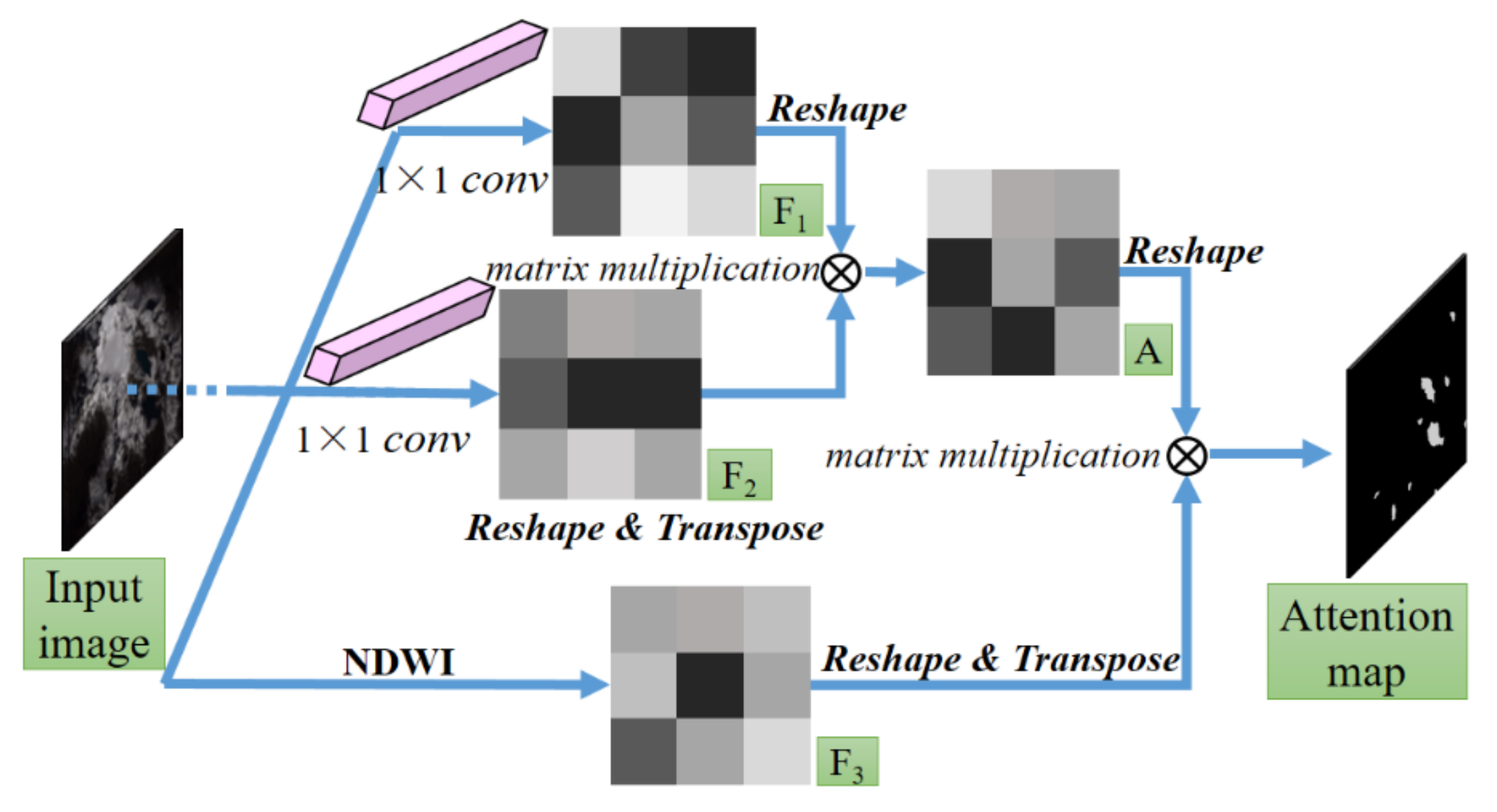
Attention mechanisms have been successfully applied in the field of image segmentation, highlighting the features that need attention based on the context of the network. Fu et al. [34] proposed a dual attention network to capture rich contextual dependencies for scene segmentation by combining local features with their global dependencies. Li et al. [35] designed a pyramid attention network, which combined an attention mechanism with a spatial pyramid to extract precise, dense object features for semantic segmentation. To optimize and stabilize the segmentation model in terms of memory and computation, an expectation–maximization attention module was developed and encapsulated into a neural network [36]. In our GAN-GL, a water index is used in the water attention module to obtain the initial glacial lake extent. Combined with convolution features, the possible lake pixels are highlighted, and potential water areas are given a relatively high weight. The structure of this module is shown in Figure 4.

Given an input Landsat-8 OLI image $I\in {ℝ}^{H\times W\times C}$, features $F_1$ and $F_2$ are calculated through the convolution operation, with a 1 × 1 kernel size $\{F_1,F_2\}\in {ℝ}^{H\times W\times 1}$. Feature $F_3$ refers to the water index. Due to the simplicity of the expression and relatively stable thresholds used for the classification of lakes [13,37], NDWI was selected in this study, as follows:

$$NDWI=\frac{{\rho }_{green}-{\rho }_{NIR}}{{\rho }_{green}+{\rho }_{NIR}}$$

(1)

where ${\rho }_{green}$ and ${\rho }_{NIR}$ represent top-of-atmosphere (TOA) reflectance values in the green and NIR bands measured by the Landsat-8 OLI sensor, respectively.

After the calculation of all the feature maps, $F_1$ and $F_2$ are both reshaped to ${ℝ}^{N\times 1}$, where $N=H\times W$. Then, matrix multiplication is performed on the reshaped $F_1$ and transpose of reshaped $F_2$, and a softmax layer is used for the normalization of the input to obtain the feature map $A\in {ℝ}^{N\times N}$.

$$A_{ji}=\frac{\exp \left(F_{1i}\otimes F_{2j}\right)}{{\displaystyle {\sum }_{i=1}^N\exp \left(F_{1i}\otimes F_{2j}\right)}}$$

(2)

The operator $\otimes$ is the ordinary matrix multiplication. Similarly, feature $F_3$ is also reshaped to ${ℝ}^{N\times 1}$, and matrix multiplication is operated on the transpose of reshaped $F_3$ and feature $A$ to enhance the water information in the water attention map $W$:

$$W_j={\displaystyle \sum _{i=1}^N(A_{ji}\otimes F_{3i})}$$

(3)

Note that here, $W\in {ℝ}^{1\times N}$ should be reshaped to ${ℝ}^{H\times W}$.

3.1.2. Image Segmentation Module

The attention results give the weight information of a pixel that belongs to a glacial lake. To fully utilize this information and further segment glacial lakes, a U-Net-based segmentation module was incorporated into the generator. Figure 3 shows that the input of this module is the element-wise product between the water attention map and Landsat imagery. We exploited five down-sampling operations to capture the lake information at different scales, each of which contains two convolution layers with a rectified linear unit (ReLU) active function and one convolution layer with a stride of 2. The ReLU function activates the input data $x$ and extends the nonlinear applications in deep learning models, which is defined as $f(x)=\max (0,x)$. An input image with a size of $H\times W\times C$ is down-sampled to $\left(H/16\right)\times \left(W/16\right)\times C’$. Because some small glacial lakes can only be extracted from shallow layers, the feature maps of the same size during down-sampling and up-sampling are concatenated, namely as skip connections, to integrate features at different scales. Finally, lake binary masks are produced by processing connection features in the last two convolution layers.

3.2. Discriminator

The inputs of the discriminator are the generated binary masks from the previous stage and the true labels of glacial lakes. Firstly, lake information is enhanced by the element-wise product between the input masks and the Landsat imagery. ResNet-152 is used as a backbone for the extraction of features from the results of the element-wise product. The corresponding output is a 2048 dimensional feature vector of a glacial lake—this is then processed by two fully convolutional layers, and fed into a single sigmoid layer to determine whether each pixel is that of a glacial lake.

3.3. Loss Function

GAN defines a competitive game between a generator and discriminator, and the final stable state of this game is evaluated by an adversarial loss function, as follows:

$$\begin{array}{ll}\underset{G}{\min } \underset{D}{\max } E_{M\sim p_{label}}& \left[\log (D(M))\right]\\ & +E_{I\sim p_{lake}}[\log (1-D(G(I)))]\end{array}$$

(4)

where $G$ and $D$ are the generator and discriminator, respectively, $I$ is the input Landsat image, and $M$ is the input mask.

However, the action of using this loss function to train the GAN model directly is unstable because it may lead to mode collapse or convergence failure [38]. Under these conditions, a loss function in WGAN-GP is employed, which places a Lipschitz constraint on the adversarial loss and penalizes the gradient norm of the adversarial loss with respect to the input binary masks. The penalty term is defined as follows:

$${{\rm E}}_{\widehat{x}\sim P_{\widehat{x}}}\left[{\left({‖\nabla \widehat{x}D(\widehat{x})‖}_2-1\right)}^2\right]$$

(5)

where $P_{\widehat{x}}$ is the uniform sampling along the lines between the pairs of points sampled from the label distribution $P_{label}$ and lake distribution $P_{lake}$.

In order to verify whether the glacial lake information can be effectively discriminated, we used an L2 loss function to represent the content loss in the discriminator to measure the similarity between image features derived from generated masks and those derived from ground truth, as follows:

$$l_{content}\left(G\right)=\frac{1}{N}{{\displaystyle \sum _{i=1}^N‖G{\left(I\right)}_i-B_i‖}}^2$$

(6)

where $B$ is the binary masks of ground truth. Finally, combining the WGAN-GP adversarial loss and content loss, our loss function can be expressed as:

$$l\left(G,D\right)=l_{adversarial}(G,D)+l_{content}(G)$$

(7)

4. Results and Discussion

4.1. Implementation Details and Evaluation Metrics

Segmentation experiments were conducted using Tensorflow 1.14 on the Python 3.7 platform. The GAN-GL dataset was split into 70% for training and 30% for validation. In the training stage, ResNet-152 in the discriminator was pre-trained on ImageNet. The training of the model was configured with a batch size of 1 for 100 epochs, and the optimizer used was AdamOptimizer, with a learning rate of 0.0001. To quantitatively evaluate the glacial lake mapping accuracy, the number of glacial lake pixels was counted using the predicted mask and the true labeled mask, and five performance indicators, Precision (P), Recall (R), Overall Accuracy (OA), F1 Score (F1), and Intersection over Union (IoU) were used. The corresponding formulations are as follows:

• P = all correctly predicted water pixels/all predicted pixels;
• R = all correctly predicted water pixels/all water pixels;
• OA = all correctly predicted pixels/all pixels;
• F1 = 2 × P × R/(P + R);
• IoU = (predicted water pixels ∩ true water pixels)/(predicted water pixels ∪ true water pixels).

4.2. Ablation Study

To investigate the effectiveness of each module in GAN-GL and its influence on the final glacial lake mapping results, an ablation study was performed. Several specific combinations of individual modules are as follows:

• ISeg: The image segmentation module in the generator (see Figure 4); the loss function is L2 loss.
• Attn + ISeg: Combines the water attention module with the image segmentation module; the loss function is L2 loss.
• ISeg + ResNet-50: Combines the image segmentation module in the generator with ResNet-50 in the discriminator; the loss function is the same as in Equation (7).
• ISeg + ResNet-101: Combines the image segmentation module with ResNet-101; the loss function is the same as in Equation (7).
• ISeg + ResNet-152: Combines the image segmentation module with ResNet-152; the loss function is the same as in Equation (7).
• Attn + ISeg + ResNet-50: Combines the water attention and the image segmentation module in the generator, with ResNet-50 in discriminator; the loss function is the same as in Equation (7).
• Attn + ISeg + ResNet-101: Combines the water attention and the image segmentation module in the generator, with ResNet-101 in discriminator; the loss function is the same as in Equation (7).
• Attn + ISeg + ResNet-152: Combines the water attention and the image segmentation module in the generator, with ResNet-152 in discriminator; the loss function is the same as in Equation (7).

The results of the ablation study are shown in

Table 3. Experimental results of ablation study for the three glacial lake subsets.

Dataset	Indicators	①	②	③	④	⑤	⑥	⑦	⑧
GAN-GL-R	P (%)	70.36	73.48	72.73	72.32	76.53	75.29	78.26	80.87
	R (%)	71.15	72.95	80.01	87.45	85.34	84.97	86.98	90.29
	OA (%)	99.86	99.21	99.44	99.83	99.75	99.70	99.75	99.81
	F1 (%)	71.25	72.72	75.69	78.67	76.80	79.34	81.89	84.83
	IoU (%)	54.52	57.74	61.54	65.51	66.56	66.43	70.05	74.40
GAN-GL-D	P (%)	86.69	89.14	87.01	90.11	91.85	91.29	92.93	93.34
	R (%)	80.60	86.69	87.26	88.87	89.17	87.16	89.33	92.01
	OA (%)	99.56	99.57	99.47	99.33	99.64	99.66	99.39	99.28
	F1 (%)	83.53	87.90	86.63	88.98	89.99	87.81	90.60	92.17
	IoU (%)	71.73	78.41	77.20	80.97	82.63	80.29	83.64	86.34
GAN-GL-U	P (%)	63.16	66.99	66.67	73.97	74.14	74.43	75.86	77.78
	R (%)	70.59	82.52	82.61	76.32	72.88	78.02	78.57	91.30
	OA (%)	99.20	99.78	99.88	99.85	99.83	99.89	99.89	99.89
	F1 (%)	66.17	73.46	73.30	74.63	73.01	71.62	76.70	83.50
	IoU (%)	50.58	58.67	58.46	60.16	58.11	60.59	62.86	72.41

Note: ① ISeg. ② Attn + ISeg. ③ ISeg + ResNet-50. ④ ISeg + ResNet-101. ⑤ ISeg + ResNet-152. ⑥ Attn + ISeg + ResNet-50. ⑦ Attn + ISeg + ResNet-101. ⑧ Attn + ISeg + ResNet-152.

and are based on the three GAN-GL datasets. The water attention module combined with the GAN-based structure (Attn + ISeg + ResNet-152) obtained the highest values of Precision (93.34%), Recall (92.01%), F1 score (92.17%), and IoU (86.34%).

Comparison for attention module: Because the water attention mechanism enables the model to focus on the identification of lake pixels, the water attention module markedly improves the segmentation performance of the glacial lakes (with an increase of 2~3% in accuracy).

Comparison for ResNet backbone: We tested the effects of different ResNet backbones in the discriminator, including ResNet-50, ResNet-101, and ResNet-152. Table 3 shows that the deeper the layers of the ResNet backbone, the better its performance. This can be explained by the fact that ResNet-152 records more details about glacial lakes by using deeper convolution layers compared to ResNet-101 and ResNet-50. This facilitates the accurate extraction of the complex edges of glacial lakes.

Comparison for the discriminator: Clear improvements were observed in the evaluation results when the discriminator was used (e.g., the ISeg and ISeg + ResNet backbone, the Attn + ISeg and Attn + ISeg + ResNet backbone). This is because the discriminator can guide the generator to learn the real distribution of the data.

Furthermore, it should be noted that accuracies were the highest for the density-cropped dataset, which contains sufficient glacial lake information in each patch to improve the training level of the model. This shows that the density of glacial lakes in the training data is an easily overlooked but important factor that affects the overall segmentation results.

4.3. Tests of Different Attention Modules

The purpose of the water attention module is to provide the weight information of each pixel that belongs to the glacial lake. Currently, there are many simple but effective water indexes that can extract lake areas, such as NDWI, modified normalized difference water index (MNDWI) [39], and enhanced water index (EWI) [40]. To test whether these water indexes could locate a glacial lake area accurately and be adept at computing the water attention, they were incorporated into our attention module to obtain the pixel weight; then, their ability and importance with regard to mapping glacial lakes were measured. Here, MNDWI and EWI were calculated according to the following formulas:

$$\mathrm{MNDWI}=\frac{{\rho }_{green}-{\rho }_{SWIR1}}{{\rho }_{green}+{\rho }_{SWIR1}}$$

(8)

$$\mathrm{EWI}=\frac{{\rho }_C-{\rho }_{NIR}-{\rho }_{SWIR2}}{{\rho }_C+{\rho }_{NIR}+{\rho }_{SWIR2}}$$

(9)

where ${\rho }_{green}$, ${\rho }_C$, ${\rho }_{NIR}$, ${\rho }_{SWIR1}$, and ${\rho }_{SWIR2}$ represent the TOA reflectance values in the green, cirrus, NIR, SWIR₁, and SWIR₂ bands measured by the Landsat-8 OLI sensor, respectively.

According to the analysis in Section 4.2, we chose the Attn + ISeg + ResNet-152 structure and used GAN-GL-D as our evaluation data. The accuracy statistical results using different attention modules are listed in

Table 4. Accuracy evaluation of glacial lake mapping using different attention modules.

Attention Module	P (%)	R (%)	OA (%)	F1 (%)	IoU (%)
NDWI	89.57	72.24	99.47	79.98	66.63
MNDWI	90.35	56.57	99.15	69.58	53.35
EWI	85.29	60.58	99.13	70.84	54.84
Attn_NDWI	93.34	92.01	99.28	92.17	86.34
Attn_MNDWI	91.99	86.89	99.48	88.87	80.78
Attn_EWI	91.19	85.29	99.76	87.64	78.80

. Using the water index alone achieved low accuracies for mapping glacial lakes, in particular, Recall and IoU. This means that without convolution operations, the water index can misclassify objects when pixels have feature values similar to glacial lakes. Lake areas extracted by NDWI had fewer commission errors and exhibited the highest mapping accuracy when coupled with convolution operations.

Figure 5 shows the visual evaluation of the image weight for the glacial lakes under various environmental conditions using the different water attention modules. Obviously, the use of the water index provided a high weight not only to glacial lakes, but also to melting glaciers and mountain shadows (denoted by the white ellipses in the first and third rows). With added convolution operations in the water attention module, effects from these interferences can be largely avoided. The second row in Figure 5 shows that the weight obtained by EWI is very conservative because its attention tends to the interior of a glacial lake. MNDWI obtained relatively extreme estimates, with attention tending to the exterior of a lake. Only the NDWI-derived attention was uniform and close to the glacial lake boundary.

4.4. Impact of Different Training Scales

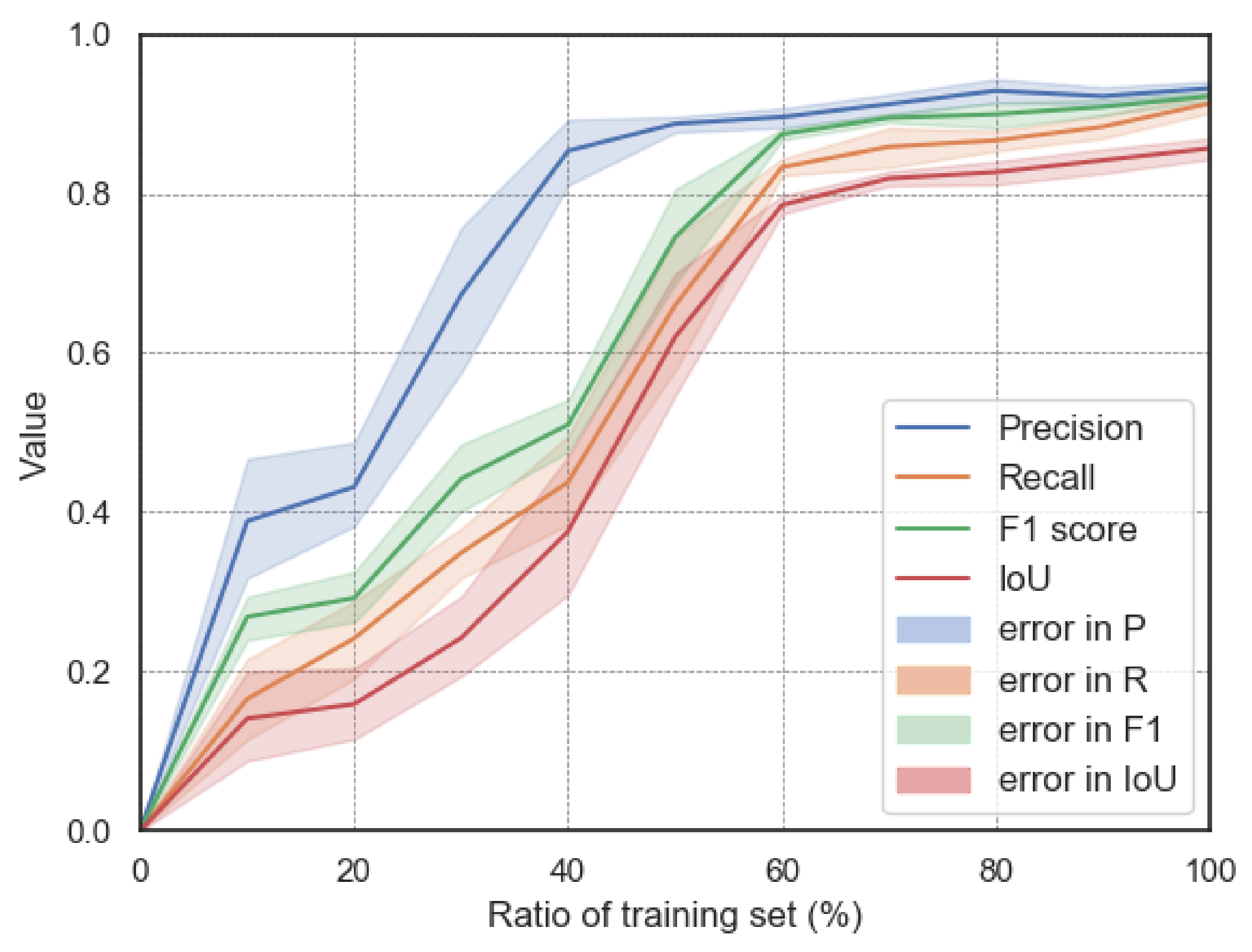
In this section, we discuss experiments conducted to survey the influence of different training scales on mapping performance. We trained the Attn+ISeg+ResNet-152 structure on progressively smaller subsets of training data and evaluated the test data from the GAN-GL-D dataset, as shown in Figure 6. Owing to slight variations in the OA, the accuracy statistics of the other four indicators with the changes of sample scale were plotted. Generally, the extraction accuracy of glacial lakes can be continuously improved with increased amounts of training data, and is particularly sensitive to the sample scale within a range of 60% of the training set. This means that a sufficient number of training samples is conducive to reliable mapping. However, when the ratio of the training set exceeds 60%, the associated accuracy increases slowly and almost reaches the saturation point.

4.5. Comparison with Other State-of-the-Art Mapping Methods

4.5.1. Experimental Materials

For a comprehensive evaluation of the robustness of the proposed model (Attn + ISeg + ResNet-152), two state-of-the-art mapping methods, the widely used global–local iterative segmentation algorithm [14] and the classical random forest classification [1], were employed for mapping performance comparison in the mapping of glacial lakes over the Eastern Himalayas. The Eastern Himalayas was chosen as our test site because this region has a high density of glacial lakes [1] and a high probability to outburst hazards [41]. Ten Landsat-8 OLI images from the year 2017 covering the entire Eastern Himalayas were used for the experiments.

The global–local iterative segmentation algorithm has been successfully used before for glacial lake mapping in mountainous areas. Implementation of the algorithm mainly consists of two steps. Firstly, potential glacial lake pixels are delineated using a global-level thresholding segmentation of NDWI coupled with NIR and SWIR bands to filter out backgrounds and noise pixels, with a spectral reflectance similar to that of glacial lakes. Secondly, a buffer zone is established for each potential lake, and then a local threshold of NDWI is used to determine the final lake extent within this buffer zone. Here, the local threshold is calculated based on the rule that the NDWI of glacial lakes and backgrounds conforms to a bimodal distribution. In our experiments, the global thresholds of NDWI ($\ge 0.10$), NIR ($<0.15$), and SWIR ($<0.05$) were set according to those of the literature [4,14,17,42]. The local-level threshold in each buffer zone is computed as follows:

$$Threshold=\frac{{\mu }_{background}\cdot {\sigma }_{water}+{\mu }_{water}\cdot {\sigma }_{background}}{{\sigma }_{water}+{\sigma }_{background}}$$

(10)

where ${\mu }_{water}$ and ${\mu }_{background}$ are the mean NDWIs of the water and background region, respectively. ${\sigma }_{water}$ and ${\sigma }_{background}$ are the variances of the NDWI of the water and background region, respectively.

The random forest is a classical ensemble learning method that employs many individual decision trees to vote for the best decision. The method has better robustness and generalization ability than methods that use an individual decision tree due to the random sampling of input data and the random subset of features. Random forest has been widely applied in the field of lake mapping [1,43]. In this study, we grew 100 trees and randomly selected 1000 pixels from the NDWI, NIR, and SWIR for glacial lakes and non-glacial lakes to train the classifier. Note that to alleviate the effects from terrain conditions, additional experiments were undertaken by introducing auxiliary ASTER DEM data (with a spatial resolution of 30 m) for the two methods. Topographic shadows were masked using slopes larger than 15° [4,33].

4.5.2. Results and Analysis

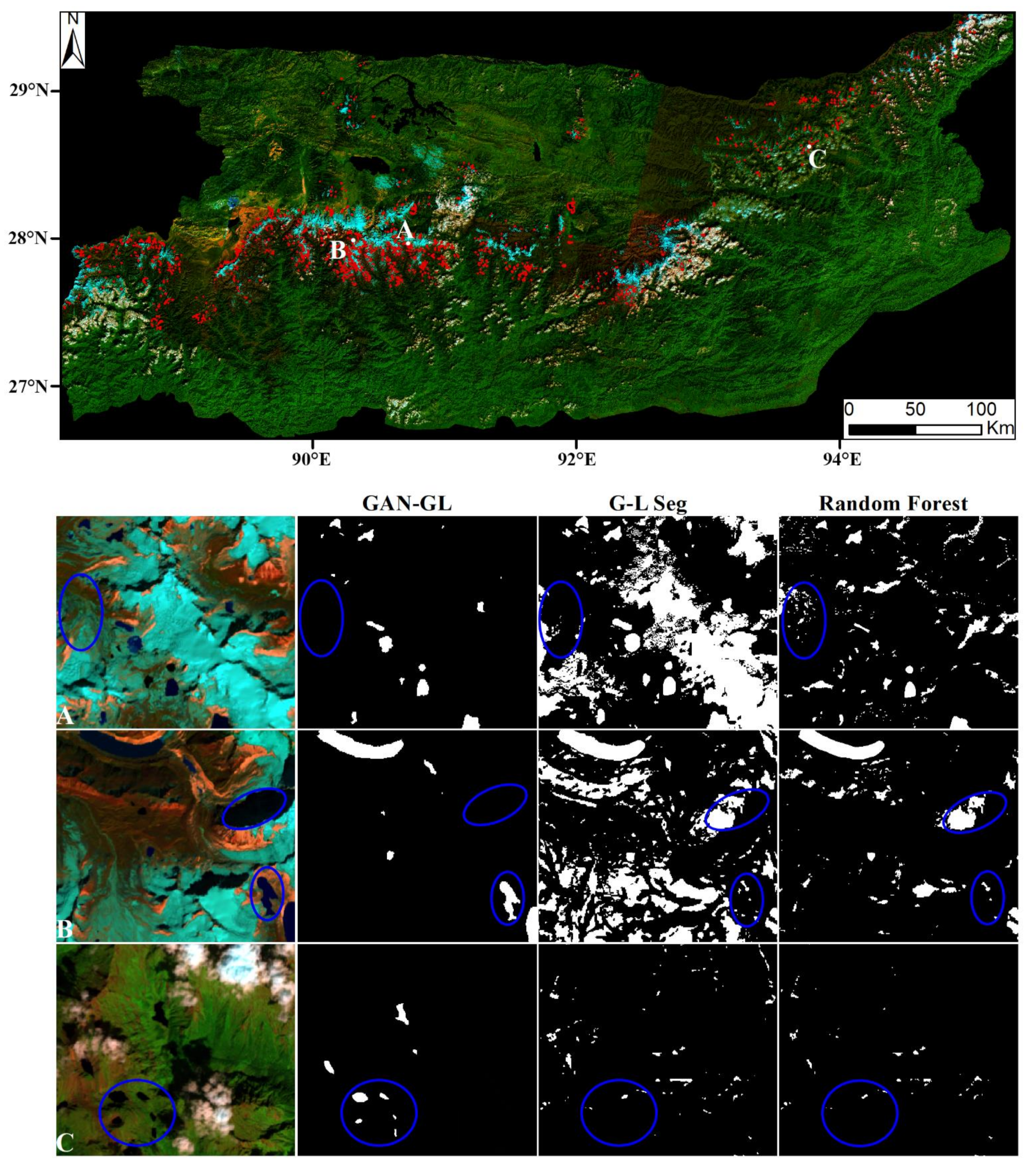
Mapping glacial lakes at a large scale is a challenging task due to the influence of various and complex climatic, geological, and terrain conditions. Figure 7 presents the spatial distribution of glacial lakes in the Eastern Himalayas. The results of GAN-GL (without DEM) and the other two methods (with DEM) are shown in the three enlarged images. In Region A, some small glacial lakes are formed around the glaciers, and the proposed GAN-GL model can extract almost all the lakes without misclassified objects. However, the lake areas obtained by the global–local iterative segmentation algorithm and random forest are affected by a high degree of noise from melting glaciers and parts of shadows, as shown in the blue ellipse. The images in Regions B and C are largely contaminated by mountain shadows, clouds, and cloud shadows, but interference from these factors was effectively eliminated by GAN-GL, meaning lakes could be easily detected, and their details preserved. However, lake areas detected by the other two methods mistakenly contained vast non-glacial lake regions, most of the glacial lakes were not precisely delineated (indicated as the blue ellipses in Region B—a lake was divided into many small parts), and the complex structure of the lake boundary was lost. Such structure comprising, for example, undulating topography, as shown in the blue ellipses in Region C. All these performances can be attributed to the fact that our GAN-GL model automatically computes numerous mid- and high-level features through convolutional operations, and employs an effective training strategy under the two constraints of content loss and adversarial loss to distinguish between different objects. Regarding the pixel-based approach, the global–local iterative segmentation algorithm is not able to effectively deal with noise pixels that have spectral values similar to those of lakes and regional heterogeneity. Random forest may have several similar decision trees that mask true results and easily overfit strong noise; this eventually leads to incomplete and noise-polluted extraction results.

Table 5. Accuracy assessment of the three mapping methods in the Eastern Himalayas.

Method	P (%)	R (%)	OA (%)	F1 (%)	IoU (%)
GAN-GL	93.19	61.07	99.85	73.31	58.46
G-L Seg (without DEM)	22.63	98.64	87.95	36.81	22.66
Random Forest (without DEM)	38.83	86.62	93.68	53.63	35.84
G-L Seg (with DEM)	44.81	88.47	96.53	59.49	42.34
Random Forest (with DEM)	57.17	74.29	96.92	64.62	47.72

shows the accuracy assessment of mapping results over the whole Eastern Himalayas. Except for Recall, other indicators obtained using the GAN-GL model are extremely high (P = 93.19%; OA = 99.85%; F1 = 73.31%; IoU = 58.46%). This means that most glacial lake pixels can be accurately extracted with only a few commission errors. Although a high Recall indicates that some lakes confused with the background are also not detected, the GAN-GL balances the effects of high accuracy and less noise and gives a good performance from other indicators. The global–local iterative segmentation algorithm achieved the highest Recall (88.47%) but the lowest Precision (44.81%) since large quantities of background pixels were also mapped. Random forest outperformed the global–local iterative segmentation algorithm for all of the indicators. However, the performance of these two methods was significantly improved with the assistance of DEM, meaning many small glacial lakes were not identified in mountainous regions.

5. Discussion

5.1. Exploration of the Improvement of the Effects of our GAN-GL Model

To obtain the accurate large-scale glacial lake mapping results in HMA, we designed this GAN-based model. As a deep learning model, there are still some possible limitations and tips to improve the generalization performance. (1) Sufficient and various data: In our study, we collected the glacial lake patches from part of HMA in a single year, and some special glacial lakes may not be sampled in our dataset. A sufficient dataset that contains lakes that vary in size, color, type, and shape can give more lake features to model to further improve the lake mapping results. (2) Adaptive input image setting: We used a Landsat series as the data source, including MSS/TM/ETM+/OLI imagery. These images give a long time series recording of glacial lakes, which is advantageous to mine the lake information. Our model only considered the inputting Landsat OLI imagery, and therefore, an adaptive input image setting would enhance the scalability for applications in other Landsat data. (3) Hierarchical structure for detecting lakes under scale variation: Scale variation in lake areas hampers the model efficiency when mapping glacial lakes in large-scale regions. The multi-level feature concatenation is an instrumental design for small object detection, but it has a huge computation cost. A hierarchical structure that detects both small lakes and large lakes has great potential for large-scale glacial lake mapping.

5.2. Performance for Different Lake Sizes

Small lakes account for a large part of the composition of glacial lakes in HMA. Statistically, in the mapping results in HMA, there are 15,456 glacial lakes (72.73%) less than 0.1 km² in 2016 [9]. These lakes are highly variable and sensitive to climate change, but are hard to identify since they are easily confused with the background.

To explore the extraction effects of our model (Attn + ISeg + ResNet-152) for different lake sizes, we counted the numbers provided with the accuracy assessment results of the glacial lakes of various sizes detected with our GAN-GL dataset and GAN-GL-D dataset, and the results can be found in

Table 6. Statistic results for different size lakes using proposed model.

Dataset	Area (km2)	<0.01 *	<0.05	<0.1	<0.2	<0.4	<0.8	≥0.8
GAN-GL-R	Count in GAN-GL	1979	1877	403	229	73	23	5
	Proportion (%)	43.12	40.90	8.78	4.99	1.59	0.50	0.11
GAN-GL-D	Count in GAN-GL	3378	1828	638	491	268	77	42
	Proportion (%)	50.26	27.19	9.49	7.31	3.99	1.15	0.61
GAN-GL-U	Count in GAN-GL	337	297	60	46	14	2	2
	Proportion (%)	44.46	39.18	7.92	6.07	1.85	0.26	0.26
Accuracy in GAN-GL-D	P (%)	-	94.12	95.85	94.96	91.47	96.68	90.70
	R (%)	-	94.07	87.61	91.10	95.31	95.93	96.34
	OA (%)	-	99.69	99.62	99.55	99.58	99.63	99.52
	F1 (%)	-	94.09	91.54	92.99	93.35	96.30	93.43
	IoU (%)	-	88.05	86.19	87.44	87.99	89.32	86.33

* Note: The accuracies of lakes less than 0.01 km² were not computed since the Hi-MAG only considered lakes greater than nine pixels (>0.0081 km²).

.

The smallest lake detected by the GAN-GL is only one pixel (area = 0.0009 km²), far smaller than the lakes in the Hi-MAG (nine pixels). This also indicates why the proportion of small lakes (<0.1 km²) is greater than that in Hi-MAG. Considering that some isolated lake pixels may be produced when splitting the lake area in the edge of cropped image patches, we kept these small lakes without conducting accuracy assessments. From Table 6, our glacial lake mapping results are almost consistent with ground truth when the lake area is greater than 0.01 km².

6. Conclusions

In this work, we proposed a generated adversarial network (GAN) for mapping glacial lakes (GAN-GL) using Landsat-8 OLI imagery. This allowed for the extraction of glacial lake information quickly and effectively with less data dependency and post-processing work. A complete glacial lake dataset was first created using random cropping, density cropping, and uniform cropping. We found that the density of glacial lakes in the training data was a factor that greatly impacted the final mapping accuracy. Then, we constructed a GAN-GL model for glacial lake mapping, which adaptively enhanced the potential lake information in a new water attention module. This module integrated the NDWI feature and spatial lake feature computed from two paralleled convolutional layers. The results of the ablation study show that our method, GAN-GL, could significantly improve the capacity to map glacial lakes, with an F1 score of 92.17% and an IoU of 86.34%. Moreover, by comparing our mapping results to those of classical global–local iterative segmentation algorithm and random forest for the entire Eastern Himalayas, the GAN-GL, with high evaluation scores, indicated that it could eliminate effects arising from mountain shadows, clouds, and melting glaciers, and automatically and precisely delineate glacial lakes. This delineation was eminently possible for many small glacial lakes under diverse environmental conditions. Our work provides a feasible way to systematically monitor and map glacial lakes over a large-scale area.

References

- Wangchuk, S.; Bolch, T. Mapping of glacial lakes using Sentinel-1 and Sentinel-2 data and a random forest classifier: Strengths and challenges. Sci. Remote Sens. 2020, 2, 100008. [Google Scholar] [CrossRef]
- Khadka, N.; Zhang, G.Q.; Thakuri, S. Glacial lakes in the Nepal Himalaya: Inventory and decadal dynamics (1977–2017). Remote Sens. 2018, 10, 1913. [Google Scholar] [CrossRef] [Green Version]
- Chand, M.B.; Watanabe, T. Development of supraglacial ponds in the Everest Region, Nepal, between 1989 and 2018. Remote Sens. 2019, 11, 1058. [Google Scholar] [CrossRef] [Green Version]
- Song, C.; Sheng, Y.; Ke, L.; Nie, Y.; Wang, J. Glacial lake evolution in the southeastern Tibetan Plateau and the cause of rapid expansion of proglacial lakes linked to glacial-hydrogeomorphic processes. J. Hydrol. 2016, 540, 504–514. [Google Scholar] [CrossRef] [Green Version]
- Wang, X.; Guo, X.Y.; Yang, C.D.; Liu, Q.H.; Wei, J.F.; Zhang, Y.; Liu, S.Y.; Zhang, Y.L.; Jiang, Z.L.; Tang, Z.G. Glacial lake inventory of High Mountain Asia (1990–2018) derived from Landsat images. Earth Syst. Sci. Data 2020, 12, 1–23. [Google Scholar] [CrossRef]
- Bohorqueza, P.; Jimenez, P.J.; Carling, P.A. Revisiting the dynamics of catastrophic late Pleistocene glacial-lake drainage, Altai Mountains, central Asia. Earth Sci. Rev. 2019, 197, 102892. [Google Scholar] [CrossRef]
- Prakash, S.; Rai, S.C.; Thakur, P.K.; Emmer, A. Inventory and recently increasing GLOF susceptibility of glacial lakes in Sikkim, Eastern Himalaya. Geomorphology 2017, 295, 39–54. [Google Scholar] [CrossRef]
- Prakash, C.; Nagarajan, R. Glacial lake changes and outburst flood hazard in Chandra basin, North-Western Indian Himalaya. Geomat. Nat. Hazards Risk 2018, 9, 337–355. [Google Scholar] [CrossRef] [Green Version]
- Petro, M.A.; Sabitov, T.Y.; Tomashevskaya, I.G.; Glazirin, G.E.; Chernomorets, S.S.; Savernyuk, E.A.; Tutubalina, O.V.; Patrokov, D.A.; Sokolov, L.S.; Dokukin, M.D.; et al. Glacial lake inventory and lake outburst potential in Uzbekistan. Sci. Total Environ. 2017, 592, 228–242. [Google Scholar] [CrossRef] [Green Version]
- Chen, F.; Zhang, M.; Guo, H.; Allen, S.; Kargel, J.S.; Haritashya, U.K.; Watson, C.S. Annual 30 m dataset for glacial lakes in High Mountain Asia from 2008 to 2017. Earth Syst. Sci. Data 2021, 13, 741–766. [Google Scholar] [CrossRef]
- Arshad, A.; Rozina, N.; Muhammad, B.I. Altitudinal dynamics of glacial lakes under changing climate in the Hindu Kush, Karakoram, and Himalaya ranges. Geomorphology 2017, 283, 72–79. [Google Scholar] [CrossRef]
- Bazai, N.A.; Cui, P.; Carling, P.A.; Wang, H.; Hassan, J.; Liu, D.; Zhang, G.; Jin, W. Increasing glacial lake outburst flood hazard in response to surge glaciers in the Karakoram. Earth Sci. Rev. 2021, 212, 103432. [Google Scholar] [CrossRef]
- McFeeters, S.K. The use of Normalized Difference Water Index (NDWI) in the delineation of open water features. Int. J. Remote Sens. 1996, 17, 1425–1432. [Google Scholar] [CrossRef]
- Li, J.L.; Sheng, Y.W. An automated scheme for glacial lake dynamics mapping using Landsat imagery and Digital Elevation Models: A Case Study in the Himalayas. Int. J. Remote Sens. 2012, 33, 5194–5213. [Google Scholar] [CrossRef]
- Shen, J.X.; Yang, L.; Chen, X.; Li, J.L.; Peng, Q.; Ju, H. A Method for Object—Oriented Automatic Extraction of Lakes in the Mountain Area from Remote Sensing Image. Remote Sens. Land Resour. 2012, 3, 84–91. [Google Scholar] [CrossRef]
- Bhardwaj, A.; Singh, M.K.; Joshi, P.K.; Snehmani; Singh, S.; Sam, L.; Gupta, R.D.; Kumar, R. A lake detection algorithm (LDA) using Landsat 8 data: A comparative approach in glacial environment. Int. J. Appl. Earth Obs. Geoinf. 2015, 38, 150–163. [Google Scholar] [CrossRef]
- Gao, Y.; Wang, W.; Yao, T.; Lu, N.; Lu, A. Hydrological network and classification of lakes on the Third Pole. J. Hydrol. 2018, 560, 582–594. [Google Scholar] [CrossRef]
- Zhao, H.; Chen, F.; Zhang, M. A Systematic Extraction Approach for Mapping Glacial lakes in High Mountain Regions of Asia. IEEE J. Sel. Top. Appl. Earth Obs. Remote Sens. 2018, 11, 2788–2799. [Google Scholar] [CrossRef]
- Li, W.; Wang, W.; Gao, X.; Wu, Y.; Wang, X.; Liu, Q. A lake extraction method in mountainous regions based on the integration of object-oriented approach and watershed algorithm. J. Geo-Inf. Sci. 2021, 23, 1272–1285. [Google Scholar] [CrossRef]
- Krizhevsky, A.; Sutskever, I.; Hinton, G. ImageNet classification with deep convolutional neural networks. In Proceedings of the Conference and Workshop on Neural Information Processing System (NIPS), Lake Tahoe, NE, USA, 3–6 December 2012. [Google Scholar]
- Long, J.; Shelhamer, E.; Darrell, T. Fully Convolutional Models for Semantic Segmentation. In Proceedings of the IEEE Conference on Computer Vision and Pattern Recognition (CVPR), Hynes Convention Center, Boston, MA, USA, 8–10 June 2015. [Google Scholar]
- Goodfellow, I.J.; Abadie, J.P.; Mirza, M.; Xu, B.; Farley, D.W.; Ozair, S.; Courvile, A.; Bengio, Y. Generative Adversarial Nets. arXiv 2014, arXiv:1406.2661. [Google Scholar]
- Qayyum, N.; Ghuffar, S.; Ahmad, H.M.; Yousaf, A.; Shahid, I. Glacial Lakes Mapping Using Multi Satellite PlanetScope Imagery and Deep Learning. ISPRS Int. J. Geo-Inf. 2020, 9, 560. [Google Scholar] [CrossRef]
- Wu, R.; Liu, G.; Zhang, R.; Wang, X.; Li, Y.; Zhang, B.; Cai, J.; Xiang, W. A Deep Learning Method for Mapping Glacial Lakes from the Combined Use of Synthetic-Aperture Radar and Optical Satellite Images. Remote Sens. 2020, 12, 4020. [Google Scholar] [CrossRef]
- Donahue, J.; Simonyan, K. Large Scale Adversarial Representation Learning. arXiv 2019, arXiv:1907.02544. [Google Scholar]
- Liu, L.; Muelly, M.; Deng, J.; Pfister, T.; Li, L. Generative Modeling for Small-Data Object Detection. In Proceedings of the International Conference on Computer Vision (ICCV), COEX Convention Center, Seoul, Korea, 27 October–2 November 2019. [Google Scholar]
- Ledig, C.; Theis, L.; Huszar, F.; Caballero, J.; Cunningham, A.; Acosta, A.; Aitken, A.; Tejani, A.; Totz, J.; Wang, Z.; et al. Photo-Realistic Single Image Super-Resolution Using a Generative Adversarial Network. arXiv 2016, arXiv:1609.04802. [Google Scholar]
- Kupyn, O.; Budzan, V.; Mykhailych, M.; Mishkin, D.; Matas, J. DeblurGAN: Blind Motion Deblurring Using Conditional Adversarial Networks. arXiv 2017, arXiv:1711.07064. [Google Scholar]
- Minaee, S.; Boykov, Y.; Porikli, F.; Plaza, A.; Kehtarnavaz, N.; Terzopoulos, D. Image Segmentation Using Deep Learning: A Survey. arXiv 2020, arXiv:2001.05566. [Google Scholar] [CrossRef] [PubMed]
- Xue, Y.; Xu, T.; Zhang, H.; Long, R.; Huang, X. SegAN: Adversarial Network with Multi-scale L1 Loss for Medical Image Segmentation. arXiv 2017, arXiv:1706.01805. [Google Scholar] [CrossRef] [PubMed] [Green Version]
- Son, J.; Park, S.J.; Jung, K.H. Retinal Vessel Segmentation in Fundoscopic Images with Generative Adversarial Networks. arXiv 2017, arXiv:1706.09318v1. [Google Scholar]
- Zhang, G.Q.; Bolch, T.; Allen, S.; Linsbauer, A.; Chen, W.; Wang, W. Glacial lake evolution and glacier–lake interactions in the Poiqu River basin, central Himalaya, 1964–2017. J. Glaciol. 2019, 65, 347–365. [Google Scholar] [CrossRef] [Green Version]
- Sheng, Y.; Song, C.; Wang, J.; Lyons, E.A.; Knox, B.R.; Cox, J.S.; Gao, F. Representative lake water extent mapping at continental scales using multi-temporal Landsat-8 imagery. Remote Sens. Environ. 2015, 185, 129–141. [Google Scholar] [CrossRef] [Green Version]
- Fu, J.; Liu, J.; Tian, H.; Li, Y.; Bao, Y.; Fang, Z.; Lu, H. Dual Attention Network for Scene Segmentation. arXiv 2018, arXiv:1809.02983. [Google Scholar]
- Li, H.; Xiong, P.; An, J.; Wang, L. Pyramid Attention Network for Semantic Segmentation. arXiv 2018, arXiv:1805.10180v1. [Google Scholar]
- Li, X.; Zhong, Z.; Wu, J.; Yang, Y.; Liu, Y. Expectation-Maximization Attention Networks for Semantic Segmentation. In Proceedings of the International Conference on Computer Vision (ICCV), COEX Convention Center, Seoul, Korea, 27 October–2 November 2019. [Google Scholar]
- Zhang, M.; Zhao, H.; Chen, F.; Zeng, J. Evaluation of effective spectral features for glacial lake mapping by using Landsat-8 OLI imagery. J. Mt. Sci. 2020, 17, 2707–2723. [Google Scholar] [CrossRef]
- Salimans, T.; Goodfellow, I.; Zaremba, W.; Cheung, W.; Radford, A.; Chen, X. Improved Techniques for Training GANs. arXiv 2016, arXiv:1606.03498. [Google Scholar]
- Xu, H.Q. Modification of normalized difference water index (NDWI) to enhance open water features in remotely sense imagery. Int. J. Remote Sens. 2006, 27, 3025–3033. [Google Scholar] [CrossRef]
- Pei, Y.; Zhang, Y.J.; Zhang, Y. A study on information extraction of water system in semi-arid regions with the Enhanced Water Index (EWI) and GIS based noise remove techniques. Remote Sens. Inf. 2007, 6, 62–67. [Google Scholar]
- Zheng, G.; Bao, A.; Allen, S.; Cánovas, J.A.B.; Yuan, Y.; Jiapaer, G.; Stoffel, M. Numerous unreported glacial lake outburst floods in the Third Pole revealed by high-resolution satellite data and geomorphological evidence. Sci. Bull. 2021, 66, 1270–1273. [Google Scholar] [CrossRef]
- Jiang, H.; Feng, M.; Zhu, Y.Q.; Lu, N.; Huang, J.; Xiao, T. An automated method for extracting rivers and lakes from Landsat imagery. Remote Sens. 2014, 6, 5067–5089. [Google Scholar] [CrossRef] [Green Version]
- Veh, G.; Korup, O.; Roessner, S.; Walz, A. Detecting Himalayan glacial lake outburst floods from 16 Landsat time series. Remote Sens. Environ. 2017, 207, 84–97. [Google Scholar] [CrossRef]
Figure 1.
Spatial location of High Mountain Asia and the distribution of 103 image tiles (red rectangles), which cover the main mountain ranges.
Figure 2.
Schematic diagram showing the three methods of creating the glacial lake subsets from the image tiles. (a) Uniform cropping: Image tiles were cropped evenly, and image patches without glacial lakes were discarded. (b) Density cropping: Image tiles were cropped according to glacial lake density. (c) Random cropping: Image tiles were cropped randomly and image patches without glacial lakes were discarded.
Figure 3.
Architecture of the proposed GAN-GL model, which mainly consists of three parts—A water attention module and an image segmentation module in the generator, and the ResNet-152-based discriminator.
Figure 4.
Structure of our water attention module.
Figure 5.
Weight results using different water attention modules. Input data are from Landsat-8 OLI images (first column, false color composites of bands 7/5/2), covering glacial lakes of various environmental components. Melting glaciers (white ellipses in the first row) and mountain shadows (white ellipses in the third row) also showed high weights using the water index alone.
Figure 6.
Accuracy for the proposed Attn+ISeg+ResNet-152 structure using different ratios of the training sets as input.
Figure 7.
Distribution of glacial lakes (marked in red contours) overlaid on Landsat-8 imagery of the Eastern Himalayas, and the compared results of the three methods. Note that the results of G-L Seg and random forest were computed using Landsat-8 imagery and DEM. Region A shows some small glacial lakes around the melting glaciers. Region B shows glacial lakes and extensive mountain shadows. Region C shows image interference from clouds and cloud shadows.