Article

Attention-Based Spatial and Spectral Network with PCA-Guided Self-Supervised Feature Extraction for Change Detection in Hyperspectral Images

1
Key Laboratory of Electronic Information Countermeasure and Simulation Technology of Ministry of Education, School of Electronic Engineering, Xidian University, No. 2 South TaiBai Road, Xi’an 710075, China
2
Academy of Advanced Interdisciplinary Research, Xidian University, No. 2 South TaiBai Road, Xi’an 710068, China
*
Author to whom correspondence should be addressed.
Remote Sens. 2021, 13(23), 4927; https://0-doi-org.brum.beds.ac.uk/10.3390/rs13234927
Submission received: 13 October 2021 / Revised: 27 November 2021 / Accepted: 30 November 2021 / Published: 4 December 2021
(This article belongs to the Special Issue Advances in Hyperspectral Data Exploitation)

Abstract

:
Joint analysis of spatial and spectral features has always been an important method for change detection in hyperspectral images. However, many existing methods cannot extract effective spatial features from the data itself. Moreover, when combining spatial and spectral features, a rough uniform global combination ratio is usually required. To address these problems, in this paper, we propose a novel attention-based spatial and spectral network with PCA-guided self-supervised feature extraction mechanism to detect changes in hyperspectral images. The whole framework is divided into two steps. First, a self-supervised mapping from each patch of the difference map to the principal components of the central pixel of each patch is established. By using the multi-layer convolutional neural network, the main spatial features of differences can be extracted. In the second step, the attention mechanism is introduced. Specifically, the weighting factor between the spatial and spectral features of each pixel is adaptively calculated from the concatenated spatial and spectral features. Then, the calculated factor is applied proportionally to the corresponding features. Finally, by the joint analysis of the weighted spatial and spectral features, the change status of pixels in different positions can be obtained. Experimental results on several real hyperspectral change detection data sets show the effectiveness and advancement of the proposed method.

1. Introduction

Change detection (CD) has been a popular research and application in the field of remote sensing in recent years, which aims to acquire the change information from multitemporal images in the same geographical area. The change information is vital in many applications, such as disaster detection and assessment [1], environmental governance [2], ecosystem monitoring [3], urban sustainable development [4,5], etc.
With the advances in sensing and imaging technology, hyperspectral images (HSIs) have attracted increasing attention and been widely utilized in earth observation applications [4,6]. Some characteristics of HSIs should be noticed: unlike multispectral images and SAR images, HSIs typically have hundreds of spectral bands, and this rich spectral information helps detect finer changes for CD. Although HSIs bring some key advantages, redundant spectral bands may introduce interference information as adjacent bands have similar spectral values, which are continuously measured by the hyperspectral sensor [4]. Moreover, the high-dimensional spectral band also leads to a significant increase in the storage and computational complexity of HSIs processing and analysis [7]. In addition, for HSIs, spatial feature extraction is more challenging than multispectral image as the serious mixed pixels phenomenon caused by low spatial resolution [8]. Furthermore, it is very difficult to obtain enough labeled training samples in HSIs analysis.
In view of the characteristics of HSIs, many approaches have been proposed for CD in HSIs. These methods can be mainly summarized into two categories:
(1) One is to directly use spectral features to obtain change information for multi-temporal HSIs. For example, Liu et al. promoted a sequential spectral change vector analysis to detect multiple changes for HSIs [9], which employs an adaptive spectral change vector representation to identify changes. Liu et al. employed spectral change information to detect change classes for achieving unsupervised HSIs change detection [10]. Different from the common method by reducing or selecting the band to reduce the band redundancy for CD in HSI, in [11], change information of each band is utilized to construct the hyperspectral change vectors for detecting multiple types of change. Recently, a general end-to-end convolutional neural network (CNN) has been proposed for HSI CD in [6], named GETNET, which introduces a unmixing-based subpixel representation to fuse multi-source information. The performance of these methods is often hindered as they usually utilize change vector analysis of spectral feature to generate directly change magnitude between multi-temporal HSIs.
(2) However, only using spectral features is bound to ignore spatial contextual information [12]. Therefore, joint spatial-spectral analysis is a common technical means in HSI-based tasks [13,14,15,16,17]. Therefore, the other is to obtain changes and improve detection accuracy through joint analysis of spectral and spatial features of HSI. For instance, Wu et al. stacked first multi-temporal HSIs, and then the local spatial information around the pixel is presented through joint sparse representation for hyperspectral anomalous CD [18]. Recently, a CD approach based on multiple morphological profiles has been proposed in HSIs [19]. This approach employed multiple morphological profiles to extract spatial information, and then a spectral angle weighted-based local absolute distance and an absolute distance are used to obtain changes. In addition, some deep learning-based techniques can help improve the performance of CD due to its ability to effectively capture and fuse spectral and spatial features. A recurrent 3D fully convolutional networks is designed to capture spectral-spatial features of HSIs simultaneously for CD in [12]. Zhan et al. promoted a three-directions spectral-spatial convolution neural network (TDSSC) in [20], which can capture representative spectra-spatial features by concatenating the feature of spectral direction and two spatial directions, and thus improving detection performance. Such methods are usually weighted to equalize spatial and spectral features to conduct joint analysis and classification, and have achieved good performance, but they usually have the following common problems:
  • The spatial features extracted by existing methods may not target for CD. For example, some methods require transfer learning from other tasks such as classification, segmentation, etc. These tasks require large-scale labeled data sets for supervised training, which increases the cost of use. There are also some methods that use autoencoders to extract the deep expression of each image. The features extracted by these two methods may not be suitable for CD. Therefore, how to extract sufficiently good spatial differential representations for CD tasks is a very critical issue.
  • Most methods adopt a uniform global weight factor when combining spatial and spectral features, that is, spatial and spectral features are analyzed according to the same ratio for each pixel at each location, which is obviously a little rough. Therefore, how to balance these two features in a task-driven adaptive way is also worth studying.
To address these two problems mentioned above, in this paper, we propose an attention-based spatial and spectral network with PCA-guided self-supervised feature extraction for CD in HSIs. The whole framework consists of two parts. In the first part, a PCA-guided self-supervised spatial feature extraction network is devised to extract spatial differential features. Concretely, two HSIs are compared to generate a difference map (DM) first. Then, the principal component analysis is utilized to obtain the transferred image that only contains several principal components. Afterwards, a mapping from the image patch, i.e., a neighborhood with a certain size for each pixel in the DM, to the corresponding principal component vector in the transferred image is established, where the spatial targeted differential features can be extracted. Finally, the extracted spatial features can be used in the subsequently joint analysis combined with the spectral features. In the whole process, no additional supervisory information is involved, and the training data used in the training only comes from the processing of the data itself, which is categorized into the self-supervised learning task recently [21,22,23]. These methods mine useful supervisory information from the data itself and can obtain performance not weaker than external supervised learning. Besides, the designed mapping relationship can make the extracted spatial features more distinctive. In the second part, we propose an attention-based spatial and spectral CD network. Different from the above-mentioned methods, the attention mechanism [24,25,26] is introduced to balance the spatial and spectral features adaptively. Specifically, the spatial and spectral features are first combined directly to calculate a weight factor for the corresponding pixel via several fully-connected layers. After that, the calculated factor is applied to weight the two features. Finally, by combining the weighted spatial and spectral features, the final change status for each pixel can be inferred. The introduction of attention mechanism enables the network to calculate its own weight factor for the spatial and spectral features of each pixel, which avoids multiple trials to select the optimal factor and allows for more detailed detection of changes. In order to improve the network performance and the detection effect, a few ground truth labels are used for semi-supervised training detection network. Experiments on several real data sets show the effectiveness and advance of our algorithm. The main contributions of our work are summarized below:
(1)
A novel PCA-guided self-supervised spatial feature extraction network, which establishes the mapping relationship from the difference to the principal components of the difference, so as to extract more specific difference representation.
(2)
The attention mechanism is introduced, which adaptively balances the proportion of spatial and spectral features, avoiding rough combination with global uniform ratio, making the model more adaptable.
(3)
We propose an innovative framework for hyperspectral image change detection, which involves a novel PCA-guided self-supervised spatial feature extraction network and an attention-based spatial-spectral fusion network. Moreover, the proposed ASSCDN can achieve the superior performance using only a small number of training samples on three widely used HSI CD datasets.
The rest of this paper is organized as follows. Related works are presented in Section 2. Section 3 describes the proposed ASSCDN in detail. In Section 4, experiments and analysis based on three pairs of HSI dataset are presented and discussed. Finally, the conclusion is provided in Section 6.

2. Related Works

2.1. Traditional CD Methods

During past few decades, many CD methods have been proposed and applied in practical applications [27,28]. In the early development of CD, two main steps are usually required to realize CD: measuring the difference image (DI) and obtaining the change detection map (CDM). Many techniques are commonly used to measure DI, such as image difference [29], image log-ratio [30], change vector analysis (CVA) [29,31], etc. Generally, these approaches calculate the change magnitude of bi-temporal images by the distance between two pixels. Afterwards, the methods widely used to generate CDM are threshold segmentation techniques (OTSU [32], expectation maximum [33]) or clustering algorithms (k-means [34], fuzzy c-means [35], k-nearest neighbors (KNN) [36], and support vector machines (SVM) [37]). With the development of CD technology, some methods are further promoted to improve the detection performance. For example, Zhuang et al. combined spectral angle mapper and change vector analysis for CD of multispectral images [38]. Thonfeld et al. proposed a robust change vector analysis (RCVA) [39] approach for multi-sensor satellite images CD. In addition to the above methods, some techniques are also helpful to improve the performance of CD, such as principal component analysis (PCA) [34,40], level set [41,42], Markov field [43,44], etc. However, these approaches rely significantly on the quality of hand-crafted features in order to measure the similarity between bi-temporal images.

2.2. Deep Learning-Based CD Methods
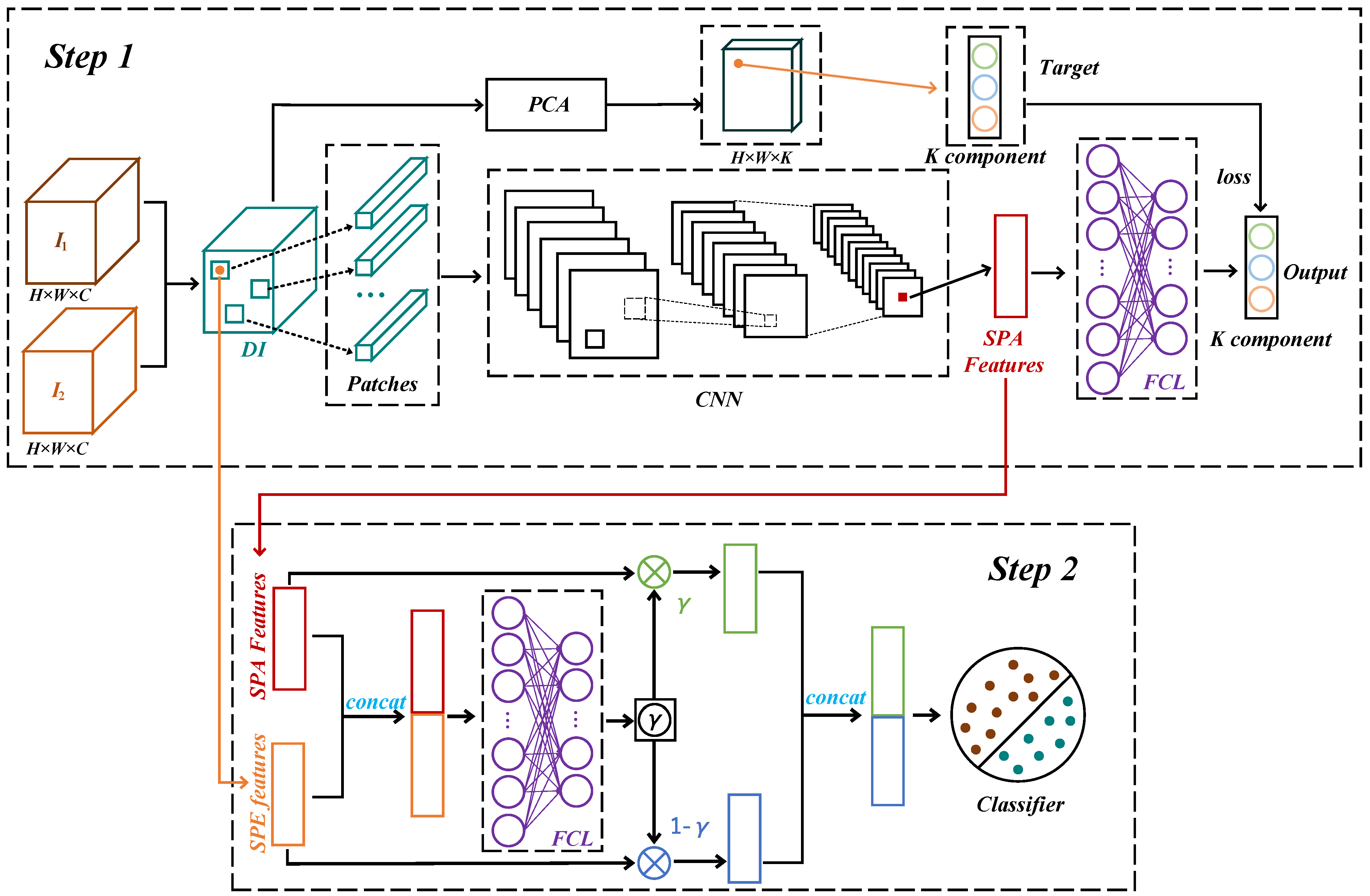
In recent years, with the booming development and wide application of deep learning technology in the field of computer vision, many scholars have extended this technology to remote sensing image CD. According to different manners of supervision, we place these deep learning-based CD approaches into three groups [28,45]: supervised CD, unsupervised CD, and semi-supervised CD.
(1) Supervised CD. This kind of method is commonly used in CD, which refers to the method of using artificially labeled samples in model training to realize supervised learning. For instance, in the early stage, Gong et al. designed a deep neural network for synthetic aperture radar (SAR) images CD, which can perform feature learning and generate CDM by supervised learning [46]. Zhang et al. recently promoted a deeply supervised image fusion network for CD, which devises a difference discrimination network to obtain CDM of bi-temporal images through deeply supervised learning [47]. Other methods are available in [48,49]. Although these supervised CD approaches can achieve acceptable performance for CD, manually labeled data is expensive and time consuming, and the quality of the manually labeled data has a significant impact on the performance of the model.
(2) Unsupervised CD. In addition to supervised learning-based CD approaches, unsupervised CD approaches have received much attention, which can acquire CDM directly without the need for manually labeled data. In recent years, many studies have been proposed for unsupervised CD, for example, Saha et al. designed an unsupervised deep change vector analysis (DCVA) method based on pretrained CNN for multiple CD [50]; an unsupervised deep slow feature analysis (DSFA) was proposed based on two symmetric deep networks for multitemporal remote sensing images in [51], which can effectively enhance the separability of changed and unchanged pixels by slow feature analysis. Moreover, other unsupervised change detection methods are available in [52,53,54,55]. However, at present, the unsupervised CD method is difficult to promote for practical application, this is because unsupervised CD approaches rely heavily on migrating features from data sources with different distribution, resulting in poor robustness and unreliable results.
(3) Semi-supervised CD. To overcome the limitation of supervised and unsupervised CD methods to a certain extent, semi-supervised learning approaches have been further developed for CD. In semi-supervised CD, in addition to a small amount of labeled data, unlabeled data are also effectively used to achieve the semi-supervised learning, and thus obtaining CDM. For example, Jiang et al. proposed a semi-supervised CD method, which extracts discriminative features by using unlabeled data and limited labeled samples [56]. In [57], a semi-supervised CNN based on a generative adversarial network was proposed, which can employ two discriminators to enhance the feature distribution consistency between the labeled and unlabeled data for CD. These semi-supervised CD methods significantly reduce the dependence on a large number of labeled data, and meanwhile maintain the performance of the model to a certain extent. However, unlabeled data may cause some interference to network training due to its unreliability, so developing reliable methods to apply unlabeled data is a crucial procedure in semi-supervised learning.

3. Proposed Method

In order to effectively detect changes based on the joint spatial and spectral features of HSIs, in this paper, we propose a novel self-supervised feature extraction and attention based CD framework, as shown in Figure 1. From the figure, it can be seen that the entire framework is divided into two steps. In the first step, the PCA-guided self-supervised spatial feature extraction network is designed, which can extract the most important change feature representation in each difference patch. In the second step, in order to effectively combine the extracted spatial and spectral features, the attention mechanism is introduced into the spatial and spectral CD network, which can adaptively learn a matching ratio for the spatial and spectral features of each patch, highlighting where is the most conducive for detecting changes. Below, we will introduce the proposed framework in detail.

3.1. Data Preparation

3.1.1. Data Preprocessing

Before comparing and analyzing the target HSIs, as the original HSIs usually contain noise and interference channels caused by atmospheric and water vapor scattering, it is often necessary to perform preprocessing such as dead pixel repair, strip removal, atmospheric correction, etc., on the original images. In addition, as change detection requires joint analysis of these two images, unaligned pixels will cause higher false detection, so joint registration of these two images is also essential.

3.1.2. Training Data Generation

It is a common method to directly analyze the difference image and obtain the final change map, since it can analyze the difference more directly and specifically. In addition, considering the lack of labeled data for HSIs, analysis based on a certain size of neighborhood of each pixel, i.e., a small patch, can often improve the reliability of change detection. After comprehensive consideration, we select the small patch centered on each pixel in the difference map of the two HSIs as the processing unit. Formally, let I 1 and I 2 represent the two HSIs of size H × W × C to be detected, where H, W, and C represent the height, width, and the number of spectral bands of the images, respectively. First, by comparing the two images, a difference map DM can be generated, i.e.,
DM = I 1 I 2 .
Then, by cutting the pixel-by-pixel neighborhood of DM, a total of H × W patches of size P × P × C can be obtained for the input of CD, where P is the patch size.

3.1.3. Principal Component Analysis (PCA) for DM

Principal component analysis (PCA) is a popular dimensional reduction machine learning technique, which has been widely used in change detection due to its simplicity, robustness, and effectiveness. For DM, PCA technique can transform the image into an orthogonal space with larger data variance, where the data can be represented by fewer dimensional features with almost little information loss, consequently finding the most expressive difference representation. Formally, for the DM data matrix D which has H × W × C samples of M-dimensional features, the transformed data can be calculated by
D = P D ,
where P is the transposed eigenvector matrix sorted according to the eigenvalue of the eigencovariance matrix C of D . That is, P satisfies the following equation:
P C P = λ 1 λ 2 λ M ,
where { λ 1 , λ 2 , , λ M } are M eigenvalues of C , which satisfies λ 1 λ 2 λ M .
In this way, the original data can be transformed into a new feature space, and the former K-dimension features can contain most of the information. The data after dimensionality reduction can be expressed as
D ˜ = T D ,
where T is the matrix of the eigenbasis vectors for the first K rows of P . Then, the obtained D ˜ can be reshaped as the dimension reduced difference map DM PCA .

3.2. PCA-Guided Self-Supervised Spatial Feature Extraction

When the data are ready, it can be fed into the designed framework for change detection. We first extract spatial features based on these patches. As DM PCA contains several major differential features, we expect to establish a mapping relationship from patch to several principal components of its central pixel. In this way, we propose a PCA-guided spatial feature extraction network (PCASFEN) which is supposed learn the spatial features that can express the most dominating features of the central pixel from the neighborhood information. There is no artificially labeled labels involved in the whole learning process; the supervised information can be obtained completely by the transformation of data itself, which is actually a self-supervised task. Specifically, given a patch with of size P × P × C , several convolutional layers are used to extract deep spatial features. In this process, a pooling layer is not used, mainly considering that the patch size is usually small and pooling may lose more spatial details. In addition, batch normalization is adopted to prevent distributed drift and thus ensure the stability of training. After the feature extraction, in order to ensure the same spatial and spectral dimensions in joint spatial and spectral analysis, the processed features are flattened and processed into a C-dimensional vector with the same feature dimensions as the input via a fully-connected layer. Finally, after several fully connected layers of processing, the output is a vector of K dimensions, which is utilized to regression-fitted with the principal component features of the central pixel of the patch.

3.3. Attention-Based Spatial and Spectral Network

At present, we have obtained spatial and spectral features representing each pixel in the DM. Joint analysis of spatial and spectral features is a common method in change detection tasks, because it can comprehensively analyze data from spatial and spectral perspectives, thus reduce isolated noise points and improve detection robustness. Generally speaking, to better balance these two features, a weighting factor γ [ 0 , 1 ] is often used. The fusion feature F of a pixel can be represented as
F = [ γ F s p a , ( 1 γ ) F s p e ] .
It can be seen that γ is a very important parameter, which is used to determine which of the spatial and spectral features contributes more to the final CD result. In most methods, a suitable γ usually requires multiple experiments to obtain, which undoubtedly greatly increases the actual use cost. In addition, for all pixels in the image, γ will eventually be set globally, but in fact, the spatial and spectral features of different pixels contribute differently to their change status. Inspired by the attention mechanism, we propose an attention-based spatial and spectral change detection network (ASSCDN). Concretely, given the spatial feature F s p a R C and a spatial feature F s p e R C of the n-th pixel in DM, first, they are concatenated as F n R 2 C , where n = 1 , 2 , , H × W . Then, F n is fed into a fully-connected layer to calculate the γ n only for the corresponding pixel, which can be expressed as
γ n = σ ( w F n + b ) = 1 1 + e ( w F n + b ) ,
where σ is the Sigmoid activation function which can ensure that γ n is between 0 and 1, and w and b represent the weight and bias of the fully-connected layer, respectively. Then, F s p a and F s p e are weighted by multiplying γ n and 1 γ n , respectively. At this time, the weighted F s p a and F s p e can be concatenated into a new feature, represented as
F n = [ γ n F s p a , ( 1 γ n ) F s p e ] .
Finally, the obtained features can be input into several fully-connected layers for classification to obtain the final change status.

3.4. Training and Testing Process

3.4.1. Training and Testing PCASFEN

As PCASFEN establishes a regression mapping from the patch to the principal component features of the central pixel, the mean square error (MSE) function is adopted as the loss of training PCASFEN. Given the input patch and feature pairs, training the PCASFEN can be seen as minimizing the MSE loss L M S E between the output K-dimensional vectors v ^ and the target principal component features v. L M S E can be represented as
L M S E = 1 N n = 1 N ( v v ^ ) 2 ,
where N is the mini-batch size. Here, the Stochastic Gradient Descent (SGD) optimizer is adopted to reduce the loss and update the network parameters. After the training of several epochs, L M S E will converge, and then the C-dimensional spatial features of each pixel neighborhood extracted from the network can be used for subsequent spatial and spectral joint analysis.

3.4.2. Training and Testing ASSCDN

For ASSCDN, it establishes the mapping from the spatial features combined with the spectral features of pixels to the final change status, which is a classification task. Therefore, the cross-entropy loss L C E function is employed to guide parameter updating. L C E can be represented as
L C E = y log ( y ^ ) ,
where y and y ^ are the ground truth label to be fitted and the output of the network, respectively. Similarly, the SGD optimizer is used to optimize the ASSCDN. Due to the effectiveness of the extracted features, only a very small number of labeled samples are enough to satisfy the training. Here, we use random selection from the reference CD map to simulate this process. The number of samples selected will be discussed in detail in the next section. After several rounds of training, the spectral features and the spatial features extracted from PCASFEN of each pixel can be directly input to the well-trained ASSCDN to obtain the change category of this pixel, and thus generate the final change map.

4. Experiments and Analysis

In this section, the experimental datasets are firstly described. Then, the experimental settings, including comparative methods and evaluation metrics are illustrated. Subsequently, the effects of different components in the proposed ASSCDN method on the detection performance are studied and analyzed. Finally, experimental results are presented and discussed in detail.

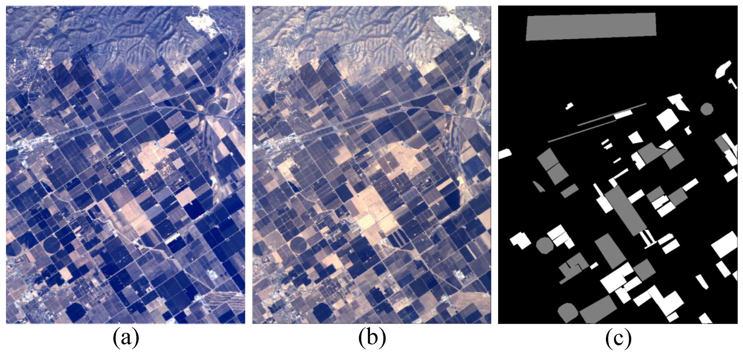
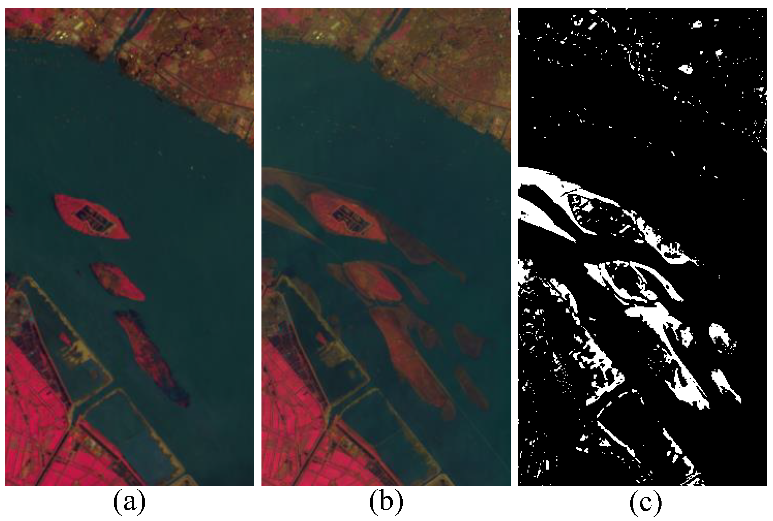
4.1. Dataset Descriptions

To evaluate the effectiveness of the proposed ASSCDN approach, three groups of HSIs are conducted in the experiments. These datasets are presented as follows.
The first and second datasets are Santa Barbara dataset and Bay Area dataset, which were released in [58]. As shown in Figure 2 and Figure 3, these datasets were captured by AVIRIS sensor, which both have 224 spectral bands. In the Santa Barbara dataset, Figure 2a,b was acquired over the Santa Barbara region, California, in 2013 and 2015, respectively. The images have 30 m/pixel spatial resolution and a size of 984 × 740 pixels. As presented in Figure 3a,b, in the Bay Area dataset, two HSIs were collected over the city of Patterson, California, in 2007 and 2015, respectively. These images are with the size of 600 × 500 pixels and the spatial resolution of 30 m/pixel. Besides, the reference images of two datasets are shown in Figure 2c and Figure 3c, which are obtained by manual interpretation, separately.
The third dataset is River dataset, which was published in [6], as shown in Figure 4. Figure 4a,b was acquired by Earth Observing-1 (EO-1) Hyperion in 3 May 2013, and 31 December 2013, respectively, which contain total 242 spectral bands, and depict a river area in Jiangsu Province, China. In the River dataset, 198 bands are employed, and these images have a size of 463 × 241 pixels and a spatial resolution of 30 m/pixel. In addition, Figure 4c provides a reference image, which is obtained by manual interpretation.

4.2. Experimental Settings

4.2.1. Evaluation Metrics

To evaluate quantitatively the accuracy of the proposed ASSCDN approach, three commonly used comprehensive evaluation metrics are selected [56,59,60], including overall accuracy (OA), F1-score ( F 1 ), and kappa coefficient (KC). Here, true positive (TP), true negative (TN), false positive (FP), and false negative (FN) are first counted by confusion matrix of the detection results, where TP indicates the number of pixels correctly detected as changed class; TN indicates the number of pixels correctly detected as unchanged class; FP and FN indicate the number of pixels falsely detected as changed and unchanged classes, respectively. On this basis, these evaluation metrics can be computed as follows:
OA = TP + TN TP + TN + FP + FN
KC = OA p e 1 p e
p e = ( TP + FP ) × RC + ( TN + FN ) × RU ( TP + TN + FP + FN ) 2
PRE = TP TP + FP
REC = TP TP + FN
F 1 = 2 × PRE × REC PRE + REC
where RC and RU represent the number of pixels that are changed and unchanged classes in the reference image, respectively. The larger values of these evaluation metrics indicate better detection performance.

4.2.2. Comparative Methods

In the experiments, eight widely used or state-of-the-art methods are selected to validate the superiority of the proposed ASSCDN approach. These methods are summarized as follows:
(1)
CVA, which is a classic method for CD, is a comprehensive measure for the differences in each spectral band [61]. Therefore, CVA is suitable for HSI CD.
(2)
KNN, aims to acquire the prediction labels of new data through the labels of the nearest K samples, which is used to acquire CDM.
(3)
SVM, a commonly applied supervised classifier, which is exploited to classify a difference image into a binary change detection map.
(4)
RCVA, was proposed by Thonfeld et al. for multi-sensor satellite images CD to improve the detection performance [39].
(5)
DCVA, can achieve an unsupervised CD based on deep change vector analysis, which implemented a pretrained CNN to extract features of bitemporal images [50].
(6)
DSFA, which employs two symmetric deep networks for multitemporal remote sensing images in [51]. This approach can effectively enhance the separability of changed and unchanged pixels by slow feature analysis.
(7)
GETNET, which is a benchmark method on River dataset [6]. This method introduces a unmixing-based subpixel representation to fuse multi-source information for HSI CD.
(8)
TDSSC, which can capture representative spectral–spatial features by concatenating the feature of spectral direction and two spatial directions, and thus improving detection performance [20].

4.2.3. Implementation Details

In the experiments, the proposed ASSCDN approach and other comparative methods were deployed on Pycharm platform with Pytorch or TensorFlow framework by using a single NVIDIA RTX 3090 or NVIDIA Tesla P40. During the training stage, the parameters of the model were optimized by a SGD optimizer with the momentum of 0.5 and the weight decay of 0.001. In all the experiments, the batch size is set as 32.

4.3. Ablation Study and Parameter Analysis on River Dataset

In this section, to investigate the effectiveness of the proposed ASSCDN, we conduct a series of ablation studies on the River dataset. These ablation studies mainly contain three aspects as follows: (1) In the proposed ASSCDN, we devise a novel PCA-guided self-supervised feature extraction network (PCASFEN) and attention-based CD framework to combine effectively the spatial and spectral features. Therefore, we first test the influence of different components on the performance of CD in the proposed ASSCDN. (2) As the patch size is an inevitable parameter in the proposed self-supervised spatial feature extraction framework, the sensitivity of patch size for network performance is investigated subsequently. (3) In addition, the relationship between the number of training samples and performance is also analyzed to validate the effectiveness of the proposed ASSCDN when only a small number of training samples are available.

4.3.1. Ablation Study for Different Components

In the ablation study, to investigate the contribution of different components in the proposed ASSCDN, three comprehensive evaluation metrics, including OA, KC, and F1, are selected to evaluate quantitatively the results of these ablation studies. Besides, to ensure the fairness of the experiment, we set the same parameter for each experiment, that is, the patch size was set as 15, the number of training samples of each class was 250, and other hyperparameter settings were the same.
In this ablation study, four major components are adopted in the our ASSCDN, i.e., “spe”, “spa”, “spe + spa”, and “spe + spa + Attention”, where “spe” denotes that only spectral features are used, “spa” denotes that only spatial features are exploited, “spe + spa” indicates that spectral features and spatial features are combined in equal proportions, and “spe + spa + Attention” indicates that spectral features and spatial features are combined through the application of the proposed attention mechanism. According to the aforementioned settings, the results were obtained on River dataset, as shown in Table 1 and Figure 5. From the quantitative results, compared with “spe”, “spa” can improve the detection performance to a certain extent, which indicates that the most important change feature representation is extracted by our proposed self-supervised spatial feature extraction framework. In addition, “spe + spa” can achieve better accuracy due to the improved discriminable feature expression by fusing spectral and spatial features, thus ameliorating the detection performance. Note that “spe + spa + Attention” reached the best accuracy (95.82%, 0.7609, and 78.37%) in terms of OA, KC, and F1. Compared with “spe + spa”, “spe + spa + Attention” was significantly improved in all three evaluation criteria (1.21%, 0.0575, and 5.10%). From the visual results, the same conclusion can be obtained. Besides, as shown in Figure 6, we also tested the performance of different components with different patch sizes, and the results further verified the contribution of the components of our proposed ASSCDN.
In summary, two aspects can be obtained by the comparison results of the above ablation study: (1) The most useful change feature representation can be captured by our proposed PCASFEN, which can help to enhance the separability between changed and unchanged classes. (2) As it is unreasonable to combine spectral and spatial features by equal proportions for different patches, a novel attention mechanism is designed to adaptively adjust the proportion of spectral and spatial features for different patches to achieve effective and reasonable fusion of spectral and spatial features, thus significantly improving the accuracy of CD. Therefore, the effectiveness of each component of the proposed ASSCDN can be validated, it can join effectively spectral and spatial features by our proposed self-supervised spatial feature extraction network and attention mechanism, thereby elevating the performance of CD for HSI.

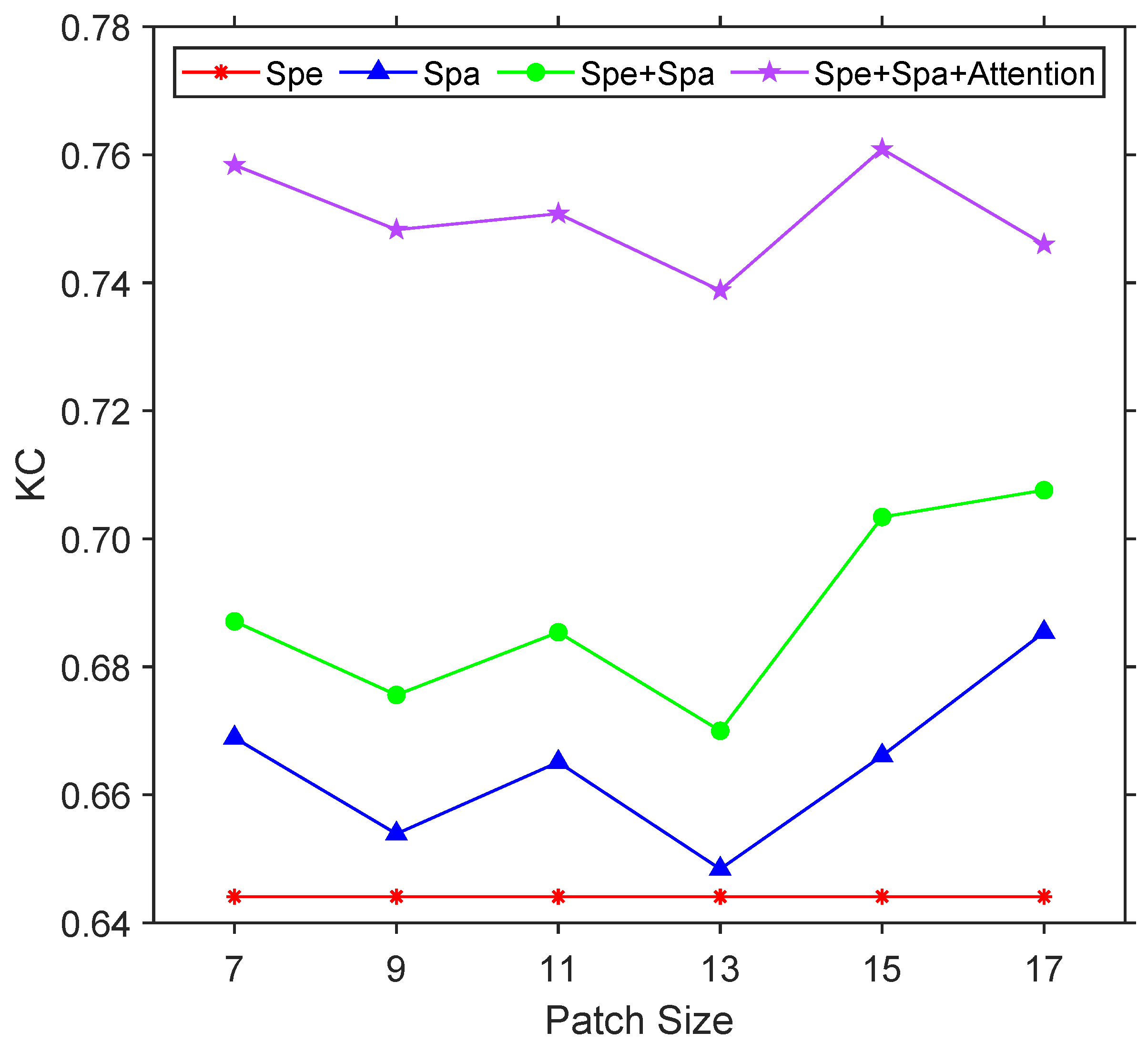
4.3.2. Sensitivity Analysis of Patch Size

In the proposed ASSCDN framework, patch size is an inevitable parameter in our PCASFEN step, which provides the spatial neighborhood information of a central pixel. Therefore, to comprehensively investigate the relationship between the patch size and accuracy, each component of our proposed ASSCDN, including “spe”, “spa”, “spe + spa”, and “spe + spa + Attention”, is employed in this experiment. Here, KC is selected to evaluate the results for each component of our proposed ASSCDN. In addition, to ensure the fairness of the comparison, in all experiments, the number of the training samples of each class was fixed to 250, and the other hyperparameter settings were the same.
Based on the above settings, the results of patch sizes ranging from 7 to 17 for each element were acquired, as presented in Figure 6. Notably, “spe” does not actually involve patch size as “spe” denotes that only spectral features are used to obtain detection results. Therefore, to facilitate comparison with the results of other components, the results of each patch size for the “spe” are the same, as the red line shown in Figure 6. By observing Figure 6, we can find that the results of “spa” present unstable fluctuation at different patch sizes. That is because different patch sizes may contain different information with various scales. Small patch sizes are more suitable for the different information of the small scale, but the extraction of the difference information of large scale is insufficient, which limits the accuracy. Similarly, larger patch size is more suitable for large-scale difference information, but for small-scale difference information, the noise may be introduced and the performance may is damaged in turn. Moreover, the relationship between the results of “spe + spa” and “spe + spa + Attention” and the patch size is similar to that of “spa”. Overall, compared with “spa” and “spe + spa”, the performance of “spe + spa + Attention” is relatively stable, and can achieve good performance in each patch size.

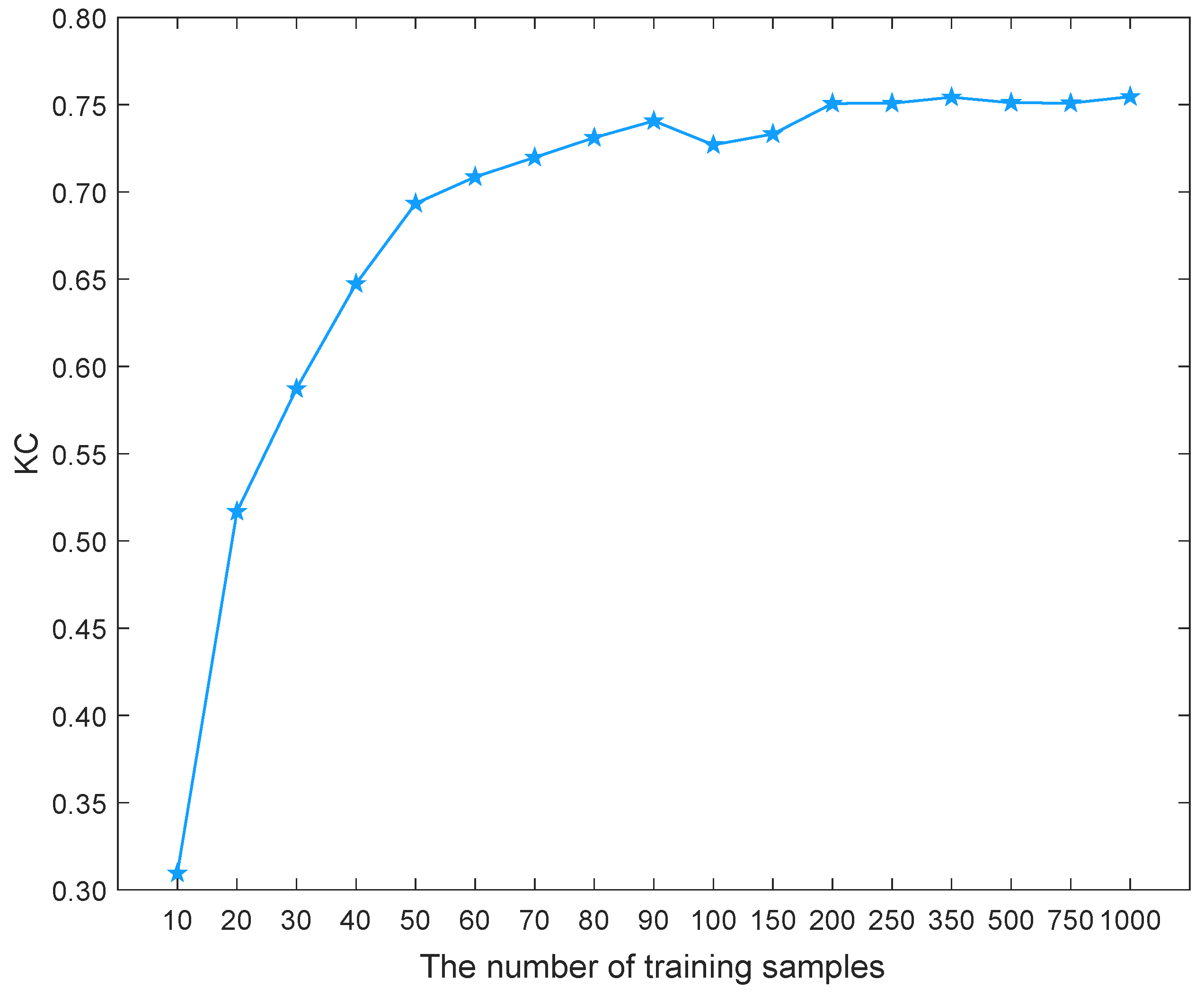
4.3.3. Analysis of the Relationship between the Number of Training Samples and Accuracy

In this subsection, to further promote the proposed ASSCDN (i.e., “spe + spa + Attention”) in practical application, we conducted an experiment to explore the relationship between the number of training samples and the accuracy. Here, when testing the performance of different numbers of training samples, we set the same hyperparameter, and the patch size was fixed at 11. Additionally, KC is employed to evaluate the accuracy of the all the results. On this basis, the results were acquired with the number of training samples ranging from 10 to 1000 (see Figure 7). As can be seen in Figure 7, with the number of training samples increasing, the value of KC increases gradually, and when the number reaches around 200, the value of KC tends to be stable. Figure 7 also reveals that the proposed ASSCDN can acquire convincing performance even with a small number of training samples.

4.4. Comparison Results and Analysis

In this section, we tested the performance of the proposed ASSCDN on three real public available HSI datasets. Moreover, to verify the superiority of the proposed ASSCDN, eight approaches are selected for comparison, including four widely used methods: CVA [61], KNN, SVM, and RCVA [39], and four deep learning-based methods: DCVA [50], DSFA [51], GETNET [6], and TDSSC [20]. Furthermore, five metrics (OA, KC, F1, PRE, and REC) are exploited to evaluate the accuracy of the proposed ASSCDN and the compared methods. Moreover, we employed a patch size of 15, and the number of the training samples of 250 to perform the proposed ASSCDN on these three datasets. In addition, to ensure the fairness of comparison, GETNET [6], and TDSSC [20] are deployed under the same semi-supervised learning framework as the proposed ASSCDN.

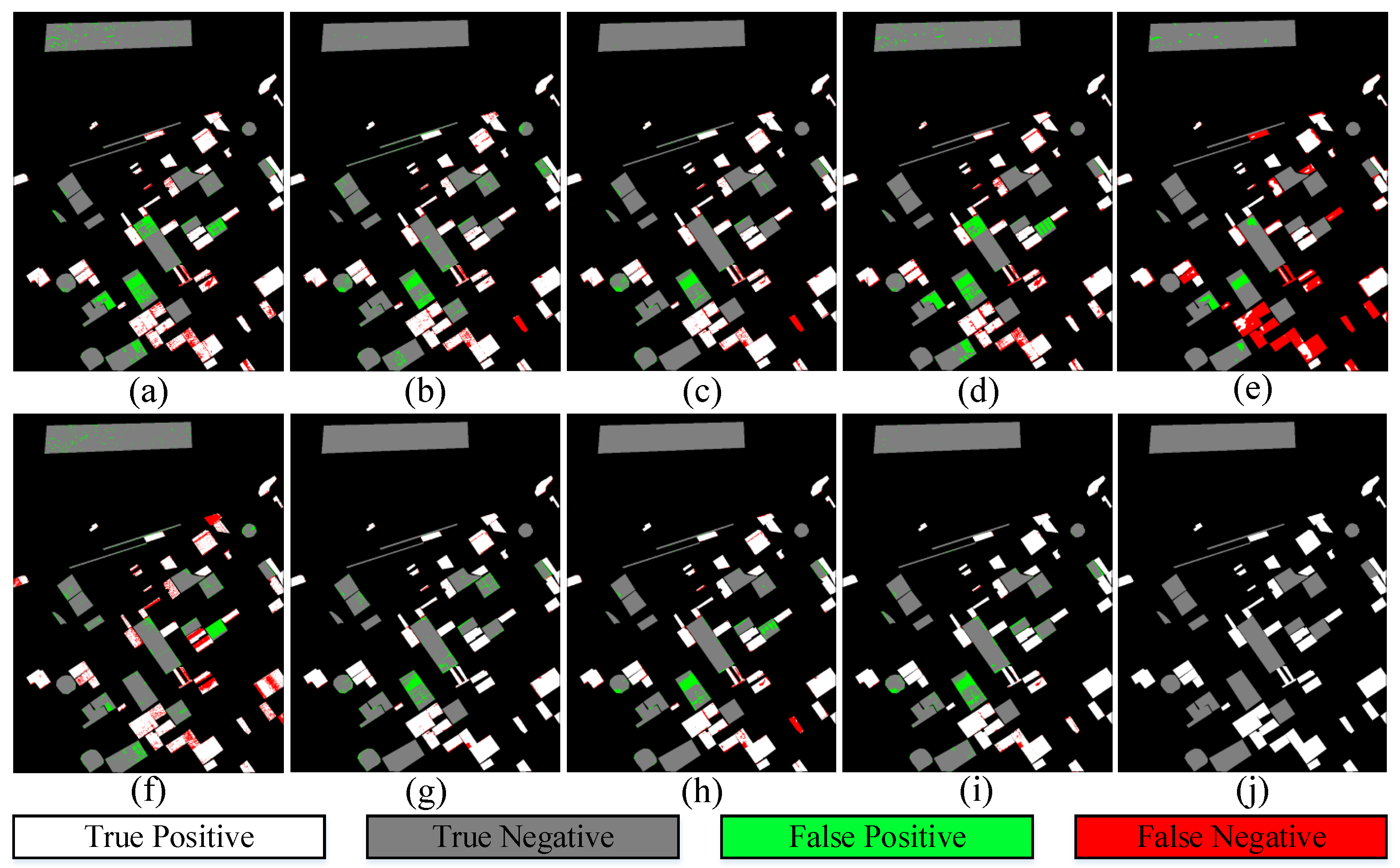
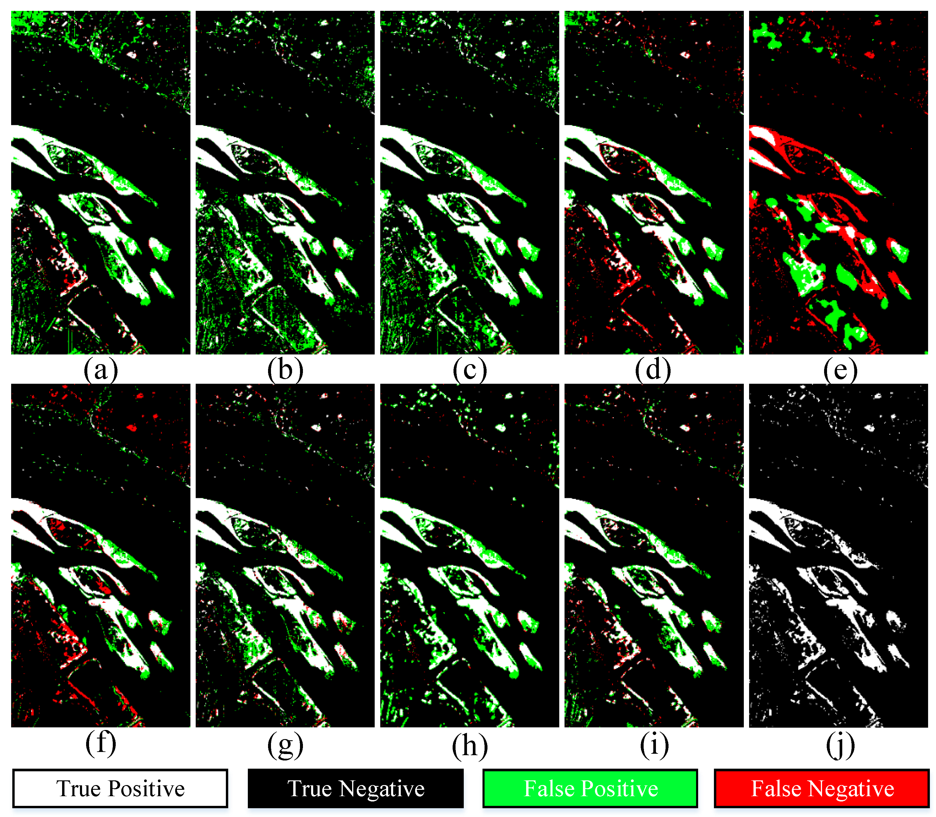
4.4.1. Results and Comparison on Barbara and Bay Datasets

The CD results were acquired by different approaches on Barbara and Bay datasets, as shown in Figure 8 and Figure 9, and the results of the quantitative evaluation are listed inTable 2 and Table 3. From Figure 8a and Figure 9a, the traditional CVA method shows more pixels of false positive due to its lack of effective use of spatial features. Different from CVA, as shown in Figure 8d and Figure 9d, although RCVA introduces neighborhood information, it is unreliable as changed targets of various scales are inevitable. Besides, KNN and SVM present fewer pixels of false positive and false negative for both Barbara and Bay datasets, especially, SVM achieved the highest PRE (93.01%), as listed in Table 2. Notably, unsupervised-based deep learning methods, i.e., DCVA and DSFA, did not reach satisfactory performance on Barbara and Bay datasets, respectively. Among them, DCVA aims to acquire CD results by comparing differences between transferred deep features, but the generalization ability of the transfer model is unreliable, while DSFA may be limited by the results of the pre-detection. GETNET [6] can obtain the second best performance on Barbara dataset, but it cannot get satisfactory accuracy on Bay data. By contrast, TDSSC [20] can achieve relatively stable accuracy on these two datasets as it captures more robust feature representation by fusing the features of spectral direction and two spatial directions. For the proposed ASSCDN, spectral and spatial features are fused adaptively for different patches, which is helpful to obtain more reliable detection results. As listed in Table 2 and Table 3, compared with the above methods, our proposed ASSCDN can achieve the best accuracy for both Barbara and Bay datasets in terms of OA, KC, and F1. From the visual results of Barbara and Bay datasets (Figure 8i and Figure 9i see), the proposed ASSCDN acquires very few pixels of false positive and false negative, and it obtains the results closest to the reference image.

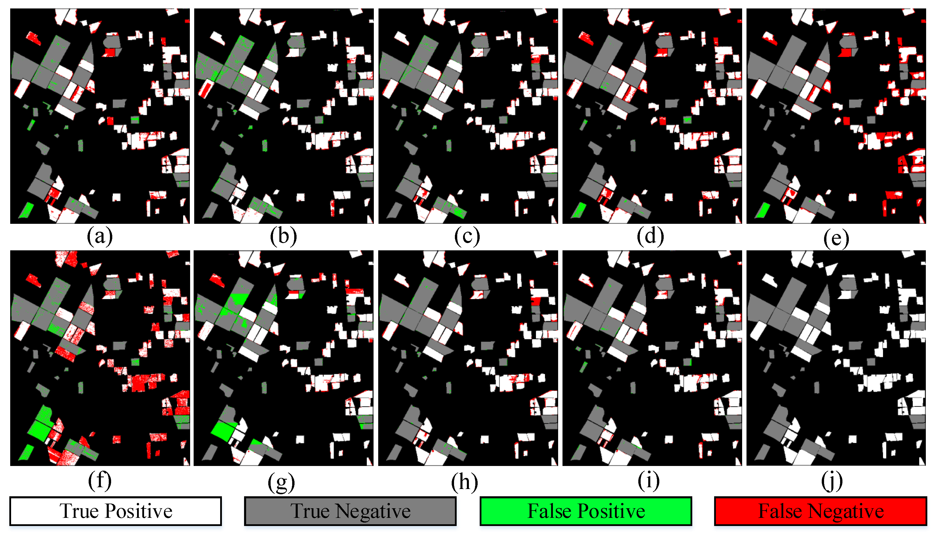
4.4.2. Results and Comparison on River Dataset

For the River dataset, as presented in Figure 4, more fine changed ground targets exist in this dataset, which increases the difficulty of obtaining fine CD results. As shown in Figure 10, the CD results were obtained by various approaches on the River dataset. From the Figure 4a–c, although typical CVA, KNN, and SVM display a few pixels of false negative, many unchanged pixels are misclassified as changed pixels as spatial information is not considered. Compared with CVA, KNN, and SVM, the result of the RCVA (see Figure 10d) shows fewer noises by introducing spatial contextual information for each pixel. By contrast, DCVA performs poorly performance, as presented in Figure 10e; this is because DCVA depends heavily on transferred deep features. For the DSFA, it generated CD result with relatively few false positive pixels but many missed detection. Both GETNET [6] and TDSSC [20] exhibit fewer false negative pixels, and compared to TDSSC [20], GETNET [6] reaches fewer false positive pixels. From the visual observations, compared with the other methods, our proposed ASSCDN presents the fewest false positive pixels, thus realizing the best visual performance. Although the proposed ASSCDN shows relatively more false negative pixels for GETNET [6] and TDSSC [20], our ASSCDN can obtain a good trade-off between false positive pixels and false negative pixels. In addition to visual comparison, quantitative comparison results have further demonstrated that the proposed ASSCDN can reach the improvements of 0.4%, 0.0113, 0.92%, and 3.47% of OA, KC, F1, and PRE, respectively, as listed in Table 4.
In summary, in this section, the aforementioned comparative experiments based on three real HSIs have been demonstrated that the proposed ASSCDN outperforms some traditional methods and state-of-the-art methods. The comparison results have further verified that effective spatial features can be captured for CD by introducing a novel PCASFEN, which can present the most significant difference representation. Furthermore, spectral and spatial features are fused in an adaptive proportion manner by exploiting an attention mechanism, which is able to enhance feature representation, and thus improves the separability of difference features.

5. Discussion

In this paper, effective ablation studies and comparison experiments are conducted on three groups of popular benchmark HSI CD datasets. In the ablation studies, three aspects can be observed. First, the effect of different components in our proposed ASSCDN has been proved that the proposed PCA-guided self-supervised feature extraction network and an attention-based CD framework can capture and fuse spatial and spectral features to further improve the performance of HSI CD. Second, although the sensitivity analysis of the patch size reveals that the patch size is more likely to affect the network accuracy (see Figure 6), the proposed ASSCDN significantly improves the accuracy of each patch size. Third, the relationship between the number of training samples and the accuracy has been explored, that is, the results show that the accuracy increases gradually with the increase of the number of training samples. In particular, the proposed ASSCDN can obtain relatively satisfactory performance when fewer training samples are employed. In addition, in the comparison experiments, eight cognate approaches, including four traditional methods (CVA [61], KNN, SVM, and RCVA [39]) and four state-of-the-art methods (DCVA [50], DSFA [51], GETNET [6], and TDSSC [20]), were selected to investigate the performance of the proposed ASSCDN. By observing the quantitative comparison, the proposed ASSCDN is superior to the other eight methods in OA, KC, and F1 for three datasets. Meanwhile, through visual comparison, it can be found that the change detection maps acquired by our ASSCDN can obtain a good trade-off between false detection and missed detection. Despite the proposed ASSCDN can provide a better result for HSI CD, the complexity of performing this method is relatively high, because the training process of our ASSCDN needs to be divided into two stages (i.e., first train the proposed self-supervised spatial feature extraction network, and then train our semi-supervised attention-based spatial and spectral network). Besides, the computational cost of our ASSCDN framework is evaluated by multiply-accumulate operations(MACs), i.e., in the PCA-guided self-supervised spatial feature extraction network step, 0.81 G MACs are needed; in the semi-supervised attention-based spatial and spectral network step, 0.0051 G MACs are needed.

6. Conclusions

In this paper, we propose an attention-based spectral and spatial change detection network (ASSCDN) for hyperspectral images, which mainly contains the following steps as follows. First, the main spatial features of differences can be extracted by our proposed PCASFEN. Second, the attention mechanism is introduced to allocate adaptively the ratio of spectral features and spatial features for fused features. Finally, by the joint analysis of the weighted spatial and spectral features, the change status of each pixel can be obtained. We conducted ablation study and parameter analysis experiment to validate the effectiveness of each component in the proposed ASSCDN. In addition, the experimental comparisons based on three groups of publicly available hyperspectral images have demonstrated that our promoted ASSCDN outperforms the other eight compared methods. In our future work, other HSIs will be collected to further investigate the robustness of this method. Furthermore, there will be a focus on weakly supervised and unsupervised HSI CD.

Author Contributions

Conceptualization, Z.W. and F.J.; methodology, Z.W.; validation, Z.W., F.J. and T.L.; investigation, F.J. and T.L.; writing—original draft preparation, Z.W., F.J. and F.X.; writing—review and editing, F.X. and P.L. All authors have read and agreed to the published version of the manuscript.

Funding

This work was supported by the National Natural Science Foundation of Shaanxi Province under Grant 2021JQ-210, the Fundamental Research Funds for the Central Universities under Grant XJS200216, and the Fundamental Research Funds for the Central Universities and the Innovation Fund of Xidian University.

Acknowledgments

We are grateful to Wang Qi and Javier López-Fandiño who provided the data for this research.

Conflicts of Interest

The authors declare no conflict of interest. The funders had no role in the design of the study; in the collection, analyses, or interpretation of data; in the writing of the manuscript, or in the decision to publish the results.

References

  1. Lu, D.; Mausel, P.; Brondizio, E.; Moran, E. Change detection techniques. Int. J. Remote Sens. 2004, 25, 2365–2401. [Google Scholar] [CrossRef]
  2. Singh, A. Review article digital change detection techniques using remotely-sensed data. Int. J. Remote Sens. 1989, 10, 989–1003. [Google Scholar] [CrossRef] [Green Version]
  3. Coppin, P.; Jonckheere, I.; Nackaerts, K.; Muys, B.; Lambin, E. Review ArticleDigital change detection methods in ecosystem monitoring: A review. Int. J. Remote Sens. 2004, 25, 1565–1596. [Google Scholar] [CrossRef]
  4. Liu, S.; Marinelli, D.; Bruzzone, L.; Bovolo, F. A review of change detection in multitemporal hyperspectral images: Current techniques, applications, and challenges. IEEE Geosci. Remote Sens. Mag. 2019, 7, 140–158. [Google Scholar] [CrossRef]
  5. ZhiYong, L.; Liu, T.; Benediktsson, J.A.; Falco, N. Land Cover Change Detection Techniques: Very-High-Resolution Optical Images: A Review. IEEE Geosci. Remote Sens. Mag. 2021, 2–21. [Google Scholar] [CrossRef]
  6. Wang, Q.; Yuan, Z.; Du, Q.; Li, X. GETNET: A general end-to-end 2-D CNN framework for hyperspectral image change detection. IEEE Trans. Geosci. Remote Sens. 2018, 57, 3–13. [Google Scholar] [CrossRef] [Green Version]
  7. Liu, S.; Du, Q.; Tong, X.; Samat, A.; Pan, H.; Ma, X. Band selection-based dimensionality reduction for change detection in multi-temporal hyperspectral images. Remote Sens. 2017, 9, 1008. [Google Scholar] [CrossRef] [Green Version]
  8. Jiang, X.; Gong, M.; Li, H.; Zhang, M.; Li, J. A two-phase multiobjective sparse unmixing approach for hyperspectral data. IEEE Trans. Geosci. Remote Sens. 2017, 56, 508–523. [Google Scholar] [CrossRef]
  9. Liu, S.; Bruzzone, L.; Bovolo, F.; Zanetti, M.; Du, P. Sequential spectral change vector analysis for iteratively discovering and detecting multiple changes in hyperspectral images. IEEE Trans. Geosci. Remote Sens. 2015, 53, 4363–4378. [Google Scholar] [CrossRef]
  10. Liu, S.; Bruzzone, L.; Bovolo, F.; Du, P. Hierarchical unsupervised change detection in multitemporal hyperspectral images. IEEE Trans. Geosci. Remote Sens. 2014, 53, 244–260. [Google Scholar]
  11. Marinelli, D.; Bovolo, F.; Bruzzone, L. A novel change detection method for multitemporal hyperspectral images based on binary hyperspectral change vectors. IEEE Trans. Geosci. Remote Sens. 2019, 57, 4913–4928. [Google Scholar] [CrossRef]
  12. Song, A.; Choi, J.; Han, Y.; Kim, Y. Change detection in hyperspectral images using recurrent 3D fully convolutional networks. Remote Sens. 2018, 10, 1827. [Google Scholar] [CrossRef] [Green Version]
  13. Zhan, T.; Gong, M.; Jiang, X.; Zhang, M. Unsupervised Scale-Driven Change Detection With Deep Spatial–Spectral Features for VHR Images. IEEE Trans. Geosci. Remote Sens. 2020, 58, 5653–5665. [Google Scholar] [CrossRef]
  14. Jiao, L.; Liang, M.; Chen, H.; Yang, S.; Liu, H.; Cao, X. Deep fully convolutional network-based spatial distribution prediction for hyperspectral image classification. IEEE Trans. Geosci. Remote Sens. 2017, 55, 5585–5599. [Google Scholar] [CrossRef]
  15. Yu, C.; Han, R.; Song, M.; Liu, C.; Chang, C.I. A simplified 2D-3D CNN architecture for hyperspectral image classification based on spatial–spectral fusion. IEEE J. Sel. Top. Appl. Earth Obs. Remote Sens. 2020, 13, 2485–2501. [Google Scholar] [CrossRef]
  16. Wang, D.; Du, B.; Zhang, L.; Xu, Y. Adaptive Spectral–Spatial Multiscale Contextual Feature Extraction for Hyperspectral Image Classification. IEEE Trans. Geosci. Remote Sens. 2020, 59, 2461–2477. [Google Scholar] [CrossRef]
  17. Hong, D.; Gao, L.; Yao, J.; Zhang, B.; Plaza, A.; Chanussot, J. Graph convolutional networks for hyperspectral image classification. IEEE Trans. Geosci. Remote Sens. 2020, 59, 5966–5978. [Google Scholar] [CrossRef]
  18. Wu, C.; Du, B.; Zhang, L. Hyperspectral anomalous change detection based on joint sparse representation. ISPRS J. Photogramm. Remote Sens. 2018, 146, 137–150. [Google Scholar] [CrossRef]
  19. Hou, Z.; Li, W.; Li, L.; Tao, R.; Du, Q. Hyperspectral change detection based on multiple morphological profiles. IEEE Trans. Geosci. Remote. Sens. 2021, 1–12. [Google Scholar] [CrossRef]
  20. Zhan, T.; Song, B.; Sun, L.; Jia, X.; Wan, M.; Yang, G.; Wu, Z. TDSSC: A Three-Directions Spectral–Spatial Convolution Neural Network for Hyperspectral Image Change Detection. IEEE J. Sel. Top. Appl. Earth Obs. Remote Sens. 2020, 14, 377–388. [Google Scholar] [CrossRef]
  21. Jing, L.; Tian, Y. Self-supervised visual feature learning with deep neural networks: A survey. IEEE Trans. Pattern Anal. Mach. Intell. 2020, 43, 4037–4058. [Google Scholar] [CrossRef]
  22. Misra, I.; Maaten, L.V.d. Self-supervised learning of pretext-invariant representations. In Proceedings of the IEEE Conference on Computer Vision Recognition, CVPR, Seattle, WA, USA, 14–19 June 2020; pp. 6707–6717. [Google Scholar]
  23. Jaiswal, A.; Babu, A.R.; Zadeh, M.Z.; Banerjee, D.; Makedon, F. A survey on contrastive self-supervised learning. Technologies 2021, 9, 2. [Google Scholar] [CrossRef]
  24. Chen, H.; Shi, Z. A spatial-temporal attention-based method and a new dataset for remote sensing image change detection. Remote Sensing 2020, 12, 1662. [Google Scholar] [CrossRef]
  25. Ghaffarian, S.; Valente, J.; Van Der Voort, M.; Tekinerdogan, B. Effect of Attention Mechanism in Deep Learning-Based Remote Sensing Image Processing: A Systematic Literature Review. Remote Sens. 2021, 13, 2965. [Google Scholar] [CrossRef]
  26. Jiang, H.; Hu, X.; Li, K.; Zhang, J.; Gong, J.; Zhang, M. Pga-siamnet: Pyramid feature-based attention-guided siamese network for remote sensing orthoimagery building change detection. Remote Sens. 2020, 12, 484. [Google Scholar] [CrossRef] [Green Version]
  27. Liu, T.; Gong, M.; Jiang, F.; Zhang, Y.; Li, H. Landslide Inventory Mapping Method Based on Adaptive Histogram-Mean Distance with Bitemporal VHR Aerial Images. IEEE Geosci. Remote Sens. Lett. 2021, 1–5. [Google Scholar] [CrossRef]
  28. You, Y.; Cao, J.; Zhou, W. A survey of change detection methods based on remote sensing images for multi-source and multi-objective scenarios. Remote Sens. 2020, 12, 2460. [Google Scholar] [CrossRef]
  29. Bruzzone, L.; Prieto, D.F. Automatic analysis of the difference image for unsupervised change detection. IEEE Trans. Geosci. Remote Sens. 2000, 38, 1171–1182. [Google Scholar] [CrossRef] [Green Version]
  30. Bazi, Y.; Bruzzone, L.; Melgani, F. An unsupervised approach based on the generalized Gaussian model to automatic change detection in multitemporal SAR images. IEEE Trans. Geosci. Remote Sens. 2005, 43, 874–887. [Google Scholar] [CrossRef] [Green Version]
  31. Chen, Q.; Chen, Y. Multi-feature object-based change detection using self-adaptive weight change vector analysis. Remote Sens. 2016, 8, 549. [Google Scholar] [CrossRef] [Green Version]
  32. Otsu, N. A threshold selection method from gray-level histograms. IEEE Trans. Syst. Man Cybern. 1979, 9, 62–66. [Google Scholar] [CrossRef] [Green Version]
  33. Bazi, Y.; Melgani, F.; Bruzzone, L.; Vernazza, G. A genetic expectation-maximization method for unsupervised change detection in multitemporal SAR imagery. Int. J. Remote Sens. 2009, 30, 6591–6610. [Google Scholar] [CrossRef]
  34. Celik, T. Unsupervised change detection in satellite images using principal component analysis and k-means clustering. IEEE Geosci. Remote Sens. Lett. 2009, 6, 772–776. [Google Scholar] [CrossRef]
  35. Shao, P.; Shi, W.; He, P.; Hao, M.; Zhang, X. Novel approach to unsupervised change detection based on a robust semi-supervised FCM clustering algorithm. Remote Sens. 2016, 8, 264. [Google Scholar] [CrossRef] [Green Version]
  36. Zhan, Y.; Fu, K.; Yan, M.; Sun, X.; Wang, H.; Qiu, X. Change detection based on deep siamese convolutional network for optical aerial images. IEEE Geosci. Remote Sens. Lett. 2017, 14, 1845–1849. [Google Scholar] [CrossRef]
  37. Migas-Mazur, R.; Kycko, M.; Zwijacz-Kozica, T.; Zagajewski, B. Assessment of Sentinel-2 Images, Support Vector Machines and Change Detection Algorithms for Bark Beetle Outbreaks Mapping in the Tatra Mountains. Remote Sens. 2021, 13, 3314. [Google Scholar] [CrossRef]
  38. Zhuang, H.; Deng, K.; Fan, H.; Yu, M. Strategies combining spectral angle mapper and change vector analysis to unsupervised change detection in multispectral images. IEEE Geosci. Remote Sens. Lett. 2016, 13, 681–685. [Google Scholar] [CrossRef]
  39. Thonfeld, F.; Feilhauer, H.; Braun, M.; Menz, G. Robust Change Vector Analysis (RCVA) for multi-sensor very high resolution optical satellite data. Int. J. Appl. Earth Obs. Geoinf. 2016, 50, 131–140. [Google Scholar] [CrossRef]
  40. Kuncheva, L.I.; Faithfull, W.J. PCA feature extraction for change detection in multidimensional unlabeled data. IEEE Trans. Neural Netw. Learn. Syst. 2013, 25, 69–80. [Google Scholar] [CrossRef]
  41. Bazi, Y.; Melgani, F.; Al-Sharari, H.D. Unsupervised change detection in multispectral remotely sensed imagery with level set methods. IEEE Trans. Geosci. Remote Sens. 2010, 48, 3178–3187. [Google Scholar] [CrossRef]
  42. Li, Z.; Shi, W.; Myint, S.W.; Lu, P.; Wang, Q. Semi-automated landslide inventory mapping from bitemporal aerial photographs using change detection and level set method. Remote Sens. Environ. 2016, 175, 215–230. [Google Scholar] [CrossRef]
  43. Gong, M.; Su, L.; Jia, M.; Chen, W. Fuzzy clustering with a modified MRF energy function for change detection in synthetic aperture radar images. IEEE Trans. Fuzzy Syst. 2013, 22, 98–109. [Google Scholar] [CrossRef]
  44. Yu, H.; Yang, W.; Hua, G.; Ru, H.; Huang, P. Change detection using high resolution remote sensing images based on active learning and Markov random fields. Remote Sens. 2017, 9, 1233. [Google Scholar] [CrossRef] [Green Version]
  45. Shi, W.; Zhang, M.; Zhang, R.; Chen, S.; Zhan, Z. Change detection based on artificial intelligence: State-of-the-art and challenges. Remote Sens. 2020, 12, 1688. [Google Scholar] [CrossRef]
  46. Gong, M.; Zhao, J.; Liu, J.; Miao, Q.; Jiao, L. Change detection in synthetic aperture radar images based on deep neural networks. IEEE Trans. Neural Netw. Learn. Syst. 2015, 27, 125–138. [Google Scholar] [CrossRef]
  47. Zhang, C.; Yue, P.; Tapete, D.; Jiang, L.; Shangguan, B.; Huang, L. A deeply supervised image fusion network for change detection in high resolution bi-temporal remote sensing images. ISPRS J. Photogramm. Remote Sens. 2020, 166, 183–200. [Google Scholar] [CrossRef]
  48. Wang, M.; Tan, K.; Jia, X.; Wang, X.; Chen, Y. A deep siamese network with hybrid convolutional feature extraction module for change detection based on multi-sensor remote sensing images. Remote Sens. 2020, 12, 205. [Google Scholar] [CrossRef] [Green Version]
  49. Lv, Z.; Liu, T.; Kong, X.; Shi, C.; Benediktsson, J.A. Landslide Inventory Mapping With Bitemporal Aerial Remote Sensing Images Based on the Dual-Path Fully Convolutional Network. IEEE J. Sel. Top. Appl. Earth Obs. Remote Sens. 2020, 13, 4575–4584. [Google Scholar] [CrossRef]
  50. Saha, S.; Bovolo, F.; Bruzzone, L. Unsupervised deep change vector analysis for multiple-change detection in VHR images. IEEE Trans. Geosci. Remote Sens. 2019, 57, 3677–3693. [Google Scholar] [CrossRef]
  51. Du, B.; Ru, L.; Wu, C.; Zhang, L. Unsupervised deep slow feature analysis for change detection in multi-temporal remote sensing images. IEEE Trans. Geosci. Remote Sens. 2019, 57, 9976–9992. [Google Scholar] [CrossRef] [Green Version]
  52. Li, X.; Yuan, Z.; Wang, Q. Unsupervised deep noise modeling for hyperspectral image change detection. Remote Sens. 2019, 11, 258. [Google Scholar] [CrossRef] [Green Version]
  53. Saha, S.; Bovolo, F.; Bruzzone, L. Building change detection in VHR SAR images via unsupervised deep transcoding. IEEE Trans. Geosci. Remote Sens. 2020, 59, 1917–1929. [Google Scholar] [CrossRef]
  54. Wu, C.; Chen, H.; Du, B.; Zhang, L. Unsupervised Change Detection in Multitemporal VHR Images Based on Deep Kernel PCA Convolutional Mapping Network. IEEE Trans. Cybern. 2021, 1–15. [Google Scholar] [CrossRef]
  55. Shao, P.; Shi, W.; Liu, Z.; Dong, T. Unsupervised change detection using fuzzy topology-based majority voting. Remote Sens. 2021, 13, 3171. [Google Scholar] [CrossRef]
  56. Jiang, F.; Gong, M.; Zhan, T.; Fan, X. A semisupervised GAN-based multiple change detection framework in multi-spectral images. IEEE Geosci. Remote Sens. Lett. 2019, 17, 1223–1227. [Google Scholar] [CrossRef]
  57. Peng, D.; Bruzzone, L.; Zhang, Y.; Guan, H.; Ding, H.; Huang, X. SemiCDNet: A semisupervised convolutional neural network for change detection in high resolution remote-sensing images. IEEE Trans. Geosci. Remote Sens. 2020, 59, 5891–5906. [Google Scholar] [CrossRef]
  58. López-Fandiño, J.; Garea, A.S.; Heras, D.B.; Argüello, F. Stacked autoencoders for multiclass change detection in hyperspectral images. In Proceedings of the 2018 IEEE International Geoscience & Remote Sensing Symposium (IGARSS), Valencia, Spain, 22–27 July 2018; IEEE: New York, NY, USA; pp. 1906–1909. [Google Scholar]
  59. Lv, Z.; Li, G.; Jin, Z.; Benediktsson, J.A.; Foody, G.M. Iterative training sample expansion to increase and balance the accuracy of land classification from VHR imagery. IEEE Trans. Geosci. Remote Sens. 2020, 59, 139–150. [Google Scholar] [CrossRef]
  60. Lv, Z.; Liu, T.; Benediktsson, J.A. Object-oriented key point vector distance for binary land cover change detection using VHR remote sensing images. IEEE Trans. Geosci. Remote Sens. 2020, 58, 6524–6533. [Google Scholar] [CrossRef]
  61. Bovolo, F.; Bruzzone, L. A theoretical framework for unsupervised change detection based on change vector analysis in the polar domain. IEEE Trans. Geosci. Remote Sens. 2006, 45, 218–236. [Google Scholar] [CrossRef] [Green Version]
Figure 1. Framework of the proposed ASSCDN. The first step is PCA-guided self-supervised spatial feature extraction network. The second step is to combine the spectral and spatial features by introducing a attention mechanism and obtain the final class.
Remotesensing 13 04927 g001
Figure 2. Barbara dataset: (a) T 1 -time image, (b) T 2 -time image, and (c) reference image. (Notation: gray color, white color, and black color denote unchanged pixels, changed pixels, and uninteresting pixels, respectively).
Remotesensing 13 04927 g002
Figure 3. Bay dataset: (a) T 1 -time image, (b) T 2 -time image, and (c) reference image. (Notation: gray color, white color, and black color denote unchanged pixels, changed pixels, and uninteresting pixels, respectively).
Remotesensing 13 04927 g003
Figure 4. River dataset: (a) T 1 -time image, (b) T 2 -time image, and (c) reference image. (Notation: white color and black color denote changed pixels and unchanged pixels, respectively).
Remotesensing 13 04927 g004
Figure 5. Visual results for ablation study of the combination of different features on the River dataset: (a) spe, (b) spa, (c) spe + spa, (d) spe + spa + Attention.
Remotesensing 13 04927 g005
Figure 6. Sensitivity analysis of patch size for each component of the proposed ASSCDN on the River dataset.
Remotesensing 13 04927 g006
Figure 7. Relationship between the number of training samples and accuracy for the proposed ASSCDN on the River dataset.
Remotesensing 13 04927 g007
Figure 8. The visual results of different methods on the Barbara dataset: (a) CVA [61], (b) KNN, (c) SVM, (d) RCVA [39], (e) DCVA [50], (f) DSFA [51], (g) GETNET [6], (h) TDSSC [20], (i) our ASSCDN, and (j) Reference image.
Remotesensing 13 04927 g008
Figure 9. The visual results of different methods on the Bay dataset: (a) CVA [61], (b) KNN, (c) SVM, (d) RCVA [39], (e) DCVA [50], (f) DSFA [51], (g) GETNET [6], (h) TDSSC [20], (i) our ASSCDN, and (j) Reference image.
Remotesensing 13 04927 g009
Figure 10. The visual results of different methods on the River dataset: (a) CVA [61], (b) KNN, (c) SVM, (d) RCVA [39], (e) DCVA [50], (f) DSFA [51], (g) GETNET [6], (h) TDSSC [20], (i) our ASSCDN, and (j) Reference image.
Remotesensing 13 04927 g010
Table 1. Quantitative comparison for ablation study of the combination of different features on the River dataset.
MethodsOA(%)KCF1 (%)
spe92.320.644168.38
spa93.600.666170.06
spe + spa94.610.703473.27
spe + spa + Attention95.820.760978.37
Table 2. Quantitative comparison results of various methods applied on the Barbara dataset.
MethodsOA (%)KCF1 (%)PRE (%)REC (%)
CVA [61]87.120.732083.9682.2685.72
KNN91.020.812288.6488.2489.05
SVM93.210.856891.2093.0189.46
RCVA [39]86.740.722683.2282.8383.62
DCVA [50]79.210.531366.9689.2453.59
DSFA [51]86.760.717469.8387.0677.92
GETNET [6]95.010.896293.8091.6296.09
TDSSC [20]94.220.878992.6792.3992.95
ASSCDN95.390.904694.3391.4597.39
Table 3. Quantitative comparison results of various methods applied on the Bay dataset.
MethodsOA (%)KCF1 (%)PRE (%)REC (%)
CVA [61]87.610.753487.4594.1681.64
KNN91.370.826891.8791.5892.16
SVM92.580.851692.8095.3590.38
RCVA [39]87.900.759887.4696.7779.79
DCVA [50]82.480.654680.6297.1968.87
DSFA [51]63.370.280058.3473.2448.48
GETNET [6]85.500.707686.8083.7390.10
TDSSC [20]94.630.892794.7398.5091.19
ASSCDN95.530.910795.6698.4593.02
Table 4. Quantitative comparison results of various methods applied on the River dataset.
MethodsOA (%)KCF1 (%)PRE (%)REC (%)
CVA [61]92.160.627266.8152.8690.76
KNN92.580.653269.1754.1595.72
SVM92.420.650468.9653.5296.92
RCVA [39]94.650.676070.5467.6273.72
DCVA [50]88.470.246630.9432.2729.72
DSFA [51]94.610.664569.4168.4470.41
GETNET [6]95.420.749677.4567.7190.45
TDSSC [20]94.290.713474.3860.9495.43
ASSCDN95.820.760978.3771.1887.18
Publisher’s Note: MDPI stays neutral with regard to jurisdictional claims in published maps and institutional affiliations.

