Article

A Comparative Study of Active Rock Glaciers Mapped from Geomorphic- and Kinematic-Based Approaches in Daxue Shan, Southeast Tibetan Plateau

1
Faculty of Geosciences and Environmental Engineering, Southwest Jiaotong University, Chengdu 611756, China
2
State-Province Joint Engineering Laboratory of Spatial Information Technology of High-Speed Rail Safety, Chengdu 611756, China
3
School of Civil Engineering and Geomatics, Southwest Petroleum University, Chengdu 610500, China
*
Author to whom correspondence should be addressed.
Remote Sens. 2021, 13(23), 4931; https://0-doi-org.brum.beds.ac.uk/10.3390/rs13234931
Submission received: 29 October 2021 / Revised: 1 December 2021 / Accepted: 1 December 2021 / Published: 4 December 2021
(This article belongs to the Special Issue Advances in SAR Image Processing and Applications)

Abstract

:
Active rock glaciers (ARGs) are important permafrost landforms in alpine regions. Identifying ARGs has mainly relied on visual interpretation of their geomorphic characteristics with optical remote sensing images, while mapping ARGs from their kinematic features has also become popular in recent years. However, a thorough comparison of geomorphic- and kinematic-based inventories of ARGs has not been carried out. In this study, we employed a multi-temporal interferometric synthetic aperture radar (InSAR) technique to derive the mean annual surface displacement velocity over the Daxue Shan, Southeast Tibet Plateau. We then compiled a rock glacier inventory by synergistically interpreting the InSAR-derived surface displacements and geomorphic features based on Google Earth images. Our InSAR-assist kinematic-based inventory (KBI) was further compared with a pre-existing geomorphic-based inventory (GBI) of rock glaciers in Daxue Shan. The results show that our InSAR-assist inventory consists of 344 ARGs, 36% (i.e., 125) more than that derived from the geomorphic-based method (i.e., 251). Only 32 ARGs in the GBI are not included in the KBI. Among the 219 ARGs detected by both approaches, the ones with area differences of more than 20% account for about 32% (i.e., 70 ARGs). The mean downslope velocities of ARGs calculated from InSAR are between 2.8 and 107.4 mm∙a−1. Our comparative analyses show that ARGs mapping from the InSAR-based kinematic approach is more efficient and accurate than the geomorphic-based approach. Nonetheless, the completeness of the InSAR-assist KBI is affected by the SAR data acquisition time, signal decorrelation, geometric distortion of SAR images, and the sensitivity of the InSAR measurement to ground deformation. We suggest that the kinematic-based approach should be utilized in future ARGs-based studies such as regional permafrost distribution assessment and water storage estimates.

1. Introduction

Rock glaciers are periglacial landforms developed in the cold mountain environment, consisting of ice and frozen rock debris that creep downslope due to the deformation of their internal ice–rock mixture [1,2]. They are visible indicators of permafrost existence in periglacial areas, and elevations at the front of rock glaciers are commonly referred to as the lower limit of discontinuous alpine permafrost [3]. Rock glaciers generally convey ice–rock mixture from the upper erosional part toward the lower depositional part (lobe) through an ill-defined transition zone (rooting zone) (Figure 5) [4], which has important hydrological and geomorphological significance in alpine regions [5,6,7]. The creeping speeds of rock glaciers are sensitive to ground-thermal conditions. The response of rock glacier kinematics to rising air temperature is thus expected to reflect the evolution of the alpine cryosphere as climate changes [8,9].
Although great efforts have been made to understand the distributions, dynamic behaviors, formation controls, and internal structures of rock glaciers [10,11,12,13,14], they are still regarded as mountain landforms with incomplete understanding [15]. Part of this poor knowledge is due to the lack of an effective approach to compile a full rock glacier inventory for a specific region [8]. Accurate inventorying and mapping of rock glaciers can reduce the uncertainty in future studies based on rock glacier inventories, such as permafrost distribution modeling and water equivalent calculation [16,17]. Currently, rock glaciers inventories can be classified into two main categories, namely “geomorphic-based approach” and “kinematic-based approach,” which are based on the interpretations of the geomorphic and kinematic features of rock glaciers, respectively [9]. Rock glacier inventories derived from these two approaches thereafter will be referred to as “geomorphic-based inventory” (GBI) and “kinematic-based inventory” (KBI).
GBI generally uses optical remote sensing images acquired by drone/satellite platforms to identify rock glaciers [11,13,18,19,20,21,22]. Typical rock glaciers are characterized by distinctive geomorphic features such as a steep front and lateral margins, ridge-and-furrow surface topography, and little vegetation on the surface. Rock glaciers can be further divided into active, transitional, and relict categories [9]. However, rock glacier inventories from the geomorphic-based approach highly depend on the expertise of operators, which may lead to a subjective identification. Previous studies [4] have found high inter-operator variability in both delineating outlines and classifying rock glaciers with the geomorphic criteria, and that variabilities between different inventories can be amplified when diverse remotely sensed images with different resolutions are used. Recent studies have introduced advanced statistical tools such as machine learning and objected-based target classification for automatically identifying rock glaciers [23,24] based on the surface geomorphic features. However, given that rock glaciers often have similar textural characteristics with their surroundings, further developments are needed for completely inventorying rock glaciers with this strategy [23,25].
KBI generally works by quantifying ground surface motion of alpine regions using geodetic techniques, from which active rock glaciers (ARGs), including the transitional ones, are then detected [9]. Geodetic techniques such as cross-correlation of optical images, interferometric synthetic aperture radar (InSAR), and differential laser scanning have been used to detect and map ARGs [6,26,27]. Among these geodetic methods, InSAR has unique superiorities with its high measurement resolution, all-day operation, and extensive coverage with low cost [28]. By combining the interpretations of phase change in SAR interferograms and geomorphic features in Google Earth images, a few studies have demonstrated the feasibility of InSAR in mapping ARGs [29,30,31,32,33,34,35].
Current studies of mapping ARGs based on the InSAR-assisted approach mostly use one or a limited number of SAR image pairs, which may generate incorrect identification of some ARGs [32]. This is mainly because the surface displacement rate detected from a SAR interferogram is confined to a certain range. ARGs with velocities lower than this range cannot be effectively identified. Furthermore, the identification of ARGs with velocities higher than this range will be affected by the SAR phase decorrelation effect. Recent studies have shown that multi-temporal InSAR can reduce SAR phase decorrelation and be used to detect the ARGs with low surface velocities [35]. Brencher, et al. [36] compiled 255 ARGs based on multi-year SAR LOS (line-of-sight) displacement velocity in the Uinta Mountains, with a velocity range from 0.88 to 5.26 cm∙a−1, demonstrating the strength of multi-temporal InSAR for ARG mapping.
Both kinematic- and geomorphic-based rock glacier inventories have their effectiveness. However, until now, a detailed evaluation of the two approaches has not been conducted. Additionally, although multi-temporal InSAR has been proven powerful in surface deformation detection, this technique has only been applied in limited alpine regions for ARGs mapping [35,36,37]. This study systematically investigates the strengths and weaknesses of kinematic- and geomorphic-based approaches to compiling rock glaciers and aims at providing practical strategies for compiling rock glaciers completely and accurately. We selected the Daxue Shan, Southeast Tibetan Plateau, as the test area because a geomorphic-based rock glacier inventory in this region has been compiled [22]. Based on Sentinel-1A ascending SAR images acquired between 2015 and 2019, we derived a five-year-long LOS mean velocity map of the study area. We then visually examined the kinematic and geomorphic features of the active landforms and mapped the ARGs in the Daxue Shan region. We also compared our InSAR-derived inventory with the previous geomorphic-based rock glacier inventory [22]. We finally discuss the feasibilities of the geomorphic- and kinematic-based approach, respectively, and give suggestions on compiling a complete and accurate ARG inventory. We also discuss the possible influences of different approaches used to inventory rock glaciers on future rock glacier-based studies such as permafrost distribution assessment and water storage estimates.

2. Study Area

2.1. Geological Overview

Daxue Shan is a mountain range in the Southeast Tibetan Plateau with an average elevation of about 4000 m a.s.l. It is also the geographical boundary of the Tibetan Plateau in the western Sichuan Basin, China (Figure 1a). Our study area is located in the middle of Daxue Shan, between 29.95°–30.58°N and 101.51°–101.95°E, indicated by the red polygon in Figure 1a. This area is of great significance in regulating the regional climate, stabilizing the ecological environment in the middle and upper reaches of the Yangtze River, conserving water resources, and preventing soil erosion.
The climate in Daxue Shan is relatively warm and rich in rainfall because the region is one of the main passages of the Indian Ocean warm current entering the Chinese hinterland. The Daofu weather station (2957 m a.s.l) in the western slope of Daxue Shan documents 613.5 mm of the mean annual precipitation and a mean annual air temperature of 8.14 °C. The climatic condition in Daxue Shan is highly conducive to the formation of maritime glaciers and periglacial landforms [38]. Additionally, this region is located at the intersection of the Songpan, Chuandian, and South China tectonic blocks, which is a transition area with complex geological structures [39]. The major exposed strata in Daxue Shan [22] is Tertiary monzogranite, whose lithological and mineralogical characteristics are favorable for the development of rock glaciers [13]. The steep terrain, combined with intense tectonic activity, drives the sediment transport processes and the development of local rock glaciers [22].

2.2. Geomorphic-Based Rock Glacier Inventory in Daxue Shan

Ran and Liu [22] inventoried 295 rock glaciers in the Daxue Shan area through visual interpretation of geomorphic characteristics from Google Earth images. The geomorphic parameters of these rock glaciers were also documented with the support of ArcGIS software [22]. The GBI from Ran and Liu [22] showed that the rock glaciers in Daxue Shan cover a total area of about 55.7 km2, with altitudes concentrating between 4300 and 4600 m a.s.l. Based on the analysis of the distributions and environment factors of rock glaciers, Ran and Liu [22] suggested that the formation and development of rock glaciers are dominantly controlled by the regional topography, climate, and lithology.
Based on the genetic criteria, rock glaciers can be further divided into moraine type and talus type. The former type generally develops downstream from the end of existing glaciers or the cirque of degraded glaciers, while the latter type often develops below the steep rock wall that is covered with perennial snow [20,30]. Ran and Liu [22] reported that the moraine-type rock glaciers account for 49% (146) of their inventory, while the talus-type account for 51% (149).

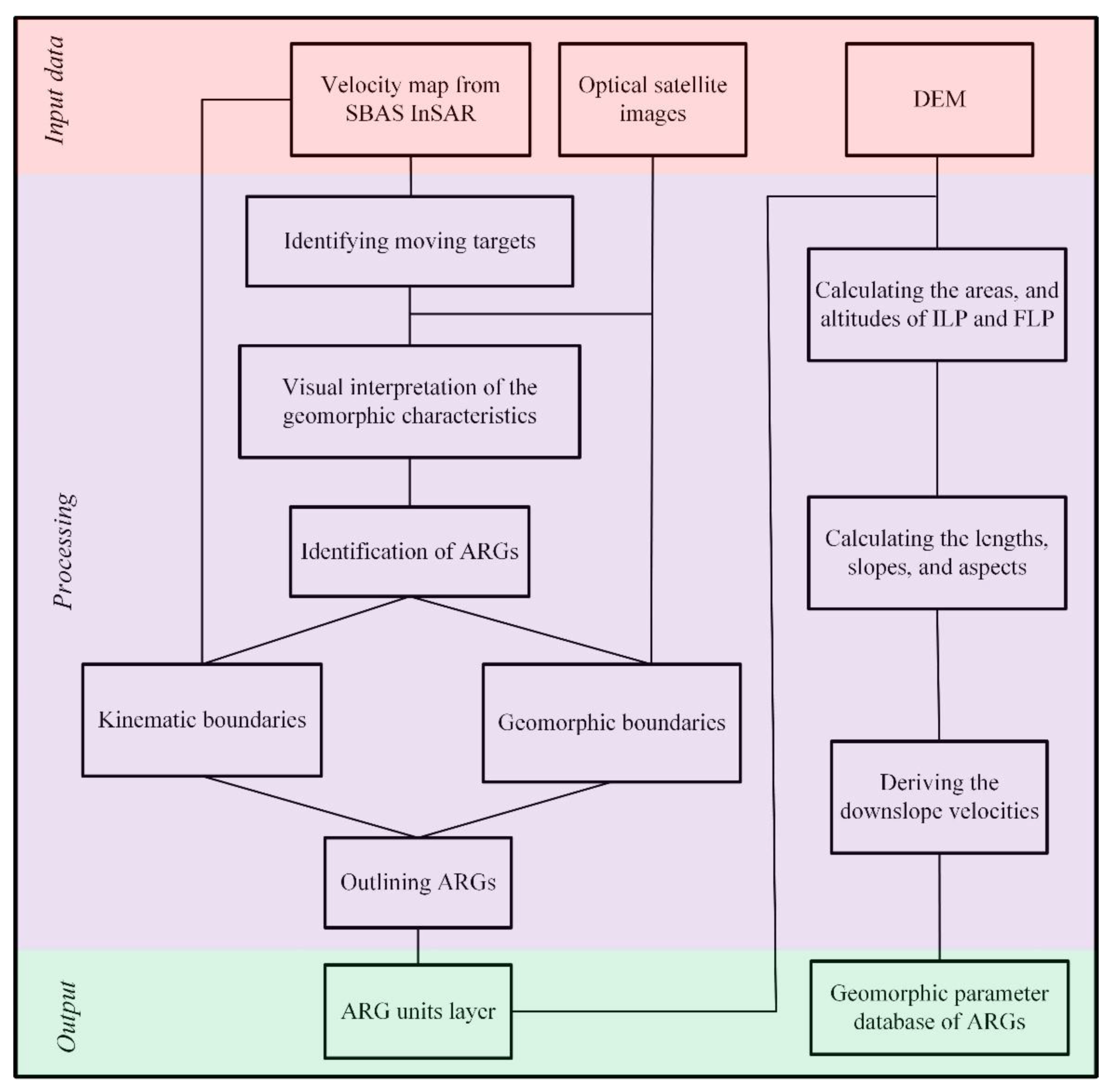
3. Remote Sensing Data and Data Processing

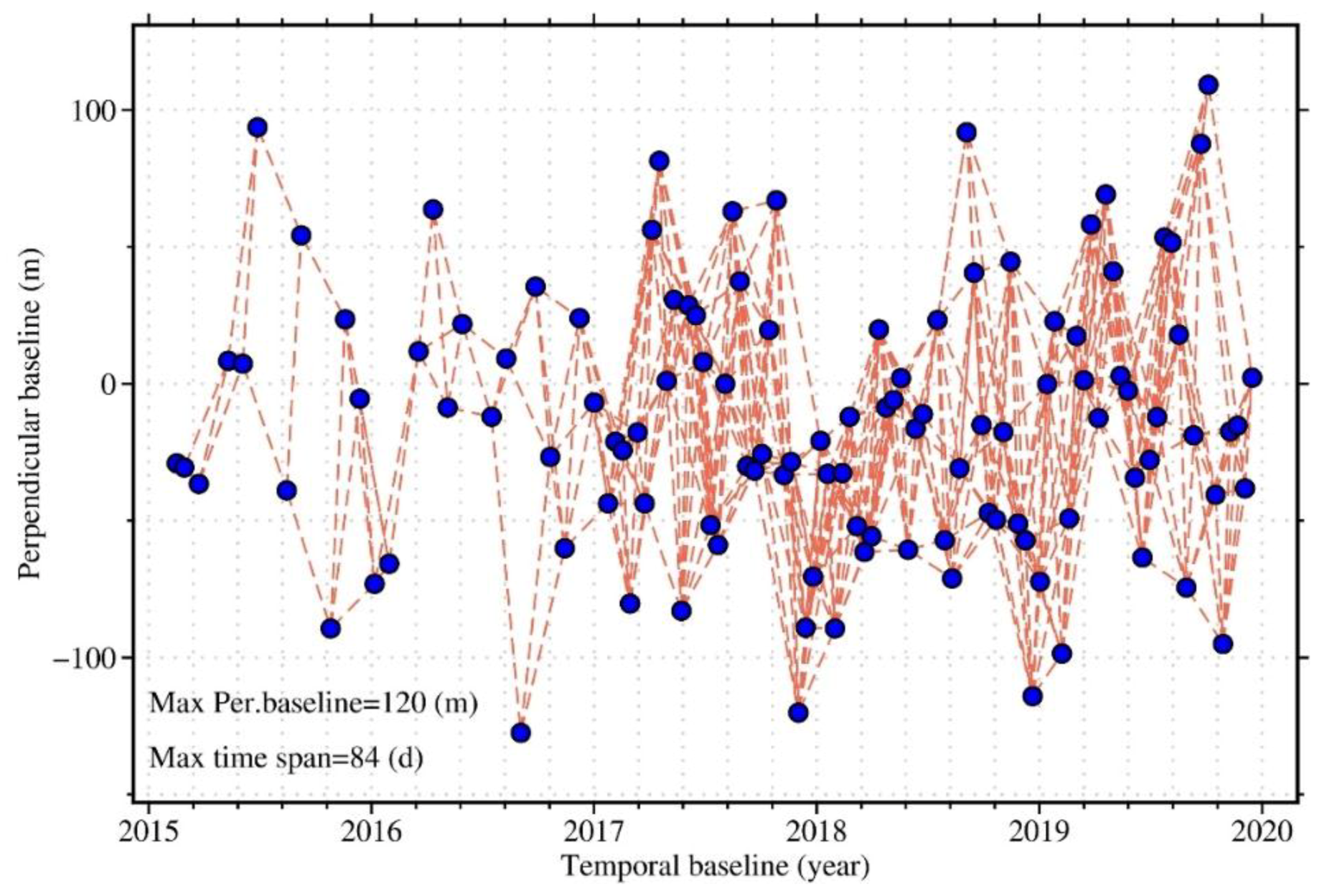
3.1. Detecting Surface Deformation with Multi-Temporal InSAR

We employed the small-baseline subset (SBAS) multi-temporal InSAR method to derive the mean surface displacement velocity of the study area based on 116 ascending Sentinel-1A SAR images acquired between 2015 and 2019. The SBAS method works by exploring the SAR phase information on distributed scatterers, which is helpful for retaining SAR interferometric phase coherence and is suitable for mapping ground displacements in alpine regions [40].
The commercial GAMMA software was used to generate SAR interferograms with main steps of image coregistration, differential phase interferometry, phase filtering, unwrapping, and terrain geocoding [41]. We set the maximum temporal baseline and spatial baseline threshold of 84 days and 120 m, respectively. We also removed the interferograms with average spatial coherence smaller than 0.65 and finally obtained a fully connected network consisting of 532 interferograms (Figure 2). The 30 m resolution AW3D30 DSM, provided by Japan Aerospace Exploration Agency (JAXA) [42], was used to circumvent the topographic phase. After generating SAR interferograms, the SAR phase was filtered using a Goldstein filter and unwrapped using a minimum cost flow algorithm. We then implemented the SBAS InSAR processing with open-source Mintpy software [43] to address mean surface displacement velocity. We used the EAR-5 products from the European Center for Medium-Range Weather Forecast to correct tropospheric phase delay [44].

3.2. Rock Glacier Mapping

With the mean ground displacement velocity map from SBAS InSAR processing available, we then mapped the ARGs in Daxue Shan using the workflow illustrated in Figure 3. First, we detected moving targets on the velocity map. A candidate moving target could be identified if at least 20–30 pixels homogenously deform [9]. We overlaid the velocity map on the optical satellite images and analyzed the geomorphic features of the moving targets to distinguish ARGs from other alpine landforms, such as glaciers, freeze–thaw mudflows, and landslides. ARGs generally develop in the lower reaches of alpine glaciers or lay at the flat section of valleys. Meanwhile, evidence of long-term downslope movements, such as transversal or longitudinal flow features, steep frontal and side slopes, and rare vegetation appearance, could be identified as distinct geomorphic features of ARGs. Here we used high-resolution Google Earth images for visual interpretation. Then, we delineated the outlines of ARGs from combined interpretations of their kinematic and geomorphic features. This was done by identifying the moving boundaries and geomorphic boundaries based on the kinematic and geomorphic features of the identified ARGs, respectively, followed by an integration of the two boundaries. Note that the interpreted boundary merely relying on the kinematic features may cause underestimation because it is common that only part of a rock glacier moves, while the interpretations only from the geomorphic features often lead to multiple results. We here chose the smallest geomorphic boundary greater than or equal to the moving boundary as the outline of an ARG.
We also calculated the geomorphic parameters (including ILP and FLP altitude, slope angle, aspect angle, area, and length) following the method proposed by Wang et al. [34]. First, the initial line point (ILP) and front line point (FLP), representing the places where permafrost creeping starts and ends of each ARG, were determined. For a detailed definition and identification method of these two points, see Section 3.3 of Wang et al. [34]. The 3D coordinates of ILPs and FLPs were extracted using the AW3D30 DSM, from which the lengths, slope angles ( θ s l p ), and the aspect angles ( α ) of ARGs were further calculated.
In addition, we used Equation (1) to convert the velocities in the SAR LOS direction ( V L O S ) into the downslope direction ( V s l p ) [31]:
V s l p = V L O S s i n ( α φ ) s i n θ i n c c o s θ s l p + c o s θ i n c s i n θ s l p
where φ is the SAR flight azimuth angle and θ i n c is the incidence angle. We calculated the mean velocity of all pixels within each ARG to represent its overall mobility. Considering the error propagation in Equation (1), we only calculated the velocities of ARGs whose conversion coefficients (i.e., the denominator part of Equation (1)) are higher than 0.2.

3.3. Comparison with the Existing Rock Glacier Inventory

To avoid biased comparison, we visually identified the ARGs from GBI made by Ran and Liu (2018) and also calculated the geomorphic parameters using the method mentioned above. We then compared the distributions, outlines, and geomorphic parameters of ARGs from the GBI with our InSAR-assist kinematic-based inventory.
Note that the GBI from Ran and Liu [22] did not contain the activity status of the rock glaciers. To compare GBI with our inventory, we identified the active and transitional rock glaciers in the GBI following the guidelines formulated by the IPA Action Group [9]. Among the 295 rock glaciers from GBI, 251 rock glaciers were classified into ARGs (including both the active and transitional ones), and the others (44) are relict rock glaciers (Figure 1b). Results were summarized into four cases: ARGs sharing the common boundary in KBI and GBI, ARGs having different outlines in KBI and GBI, ARGs only identified in KBI, and ARGs only identified in GBI (Figure 1b). Considering the relative subjectivity in mapping rock glacier outlines, the so-called common boundary of an ARG means that the polygons from two inventories have the same geomorphological structure, and the area difference is less than 20%.

4. Result

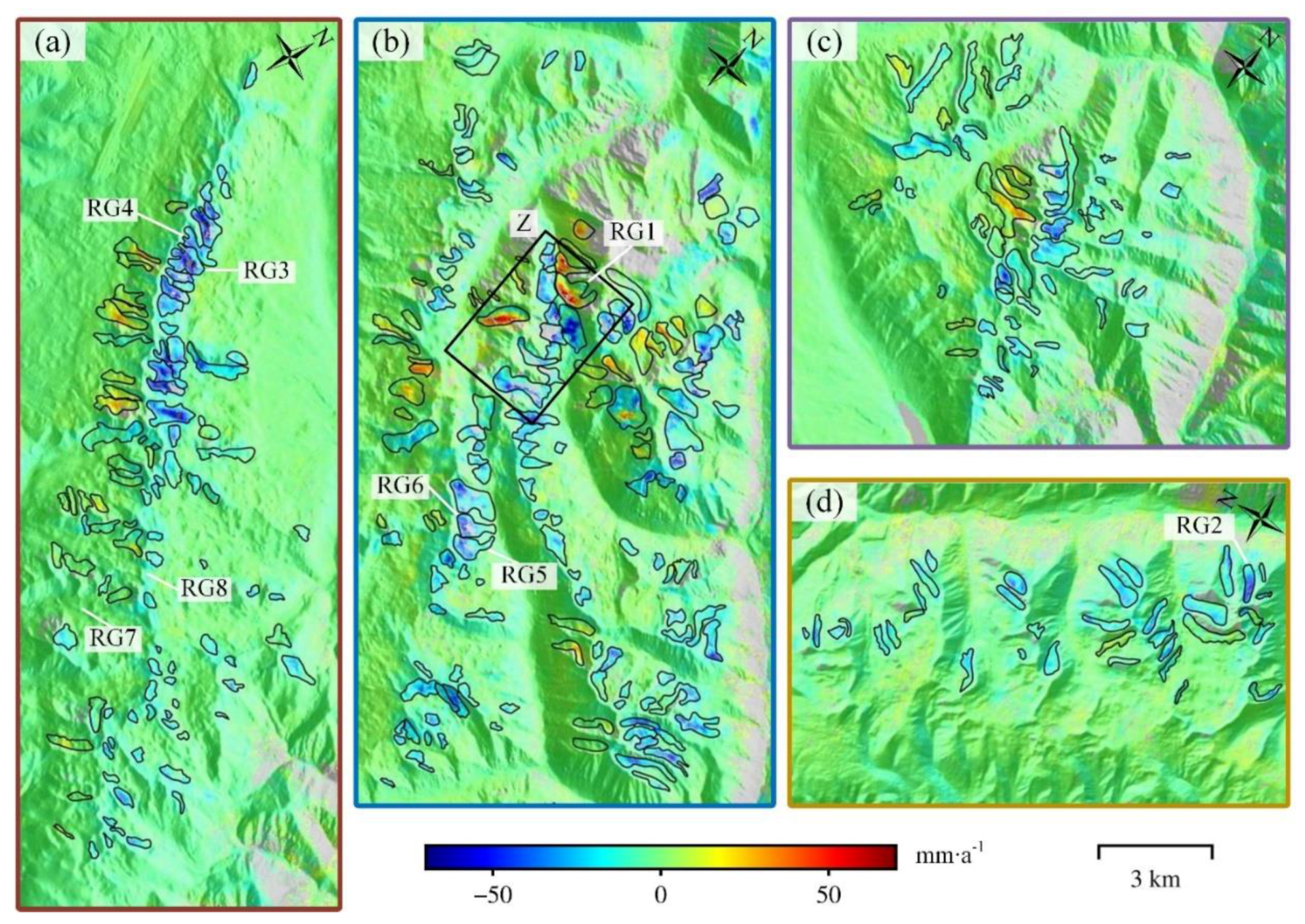
4.1. ARGs from the InSAR-Assist Kinematic-Based Inventorying

We mapped a total of 344 ARGs through the InSAR-assist kinematic-based approach in the Daxue Shan area. Figure 4 shows the outlines of ARGs from KBI overlaying on the ground surface velocity map derived from SBAS InSAR. The ARGs in the Daxue Shan region are widely distributed in the elevation range 3860–5094 m a.s.l., among which the moraine-type and talus-type ARGs account for 52% (180) and 48% (164), respectively. The ARGs mainly face the northeast.

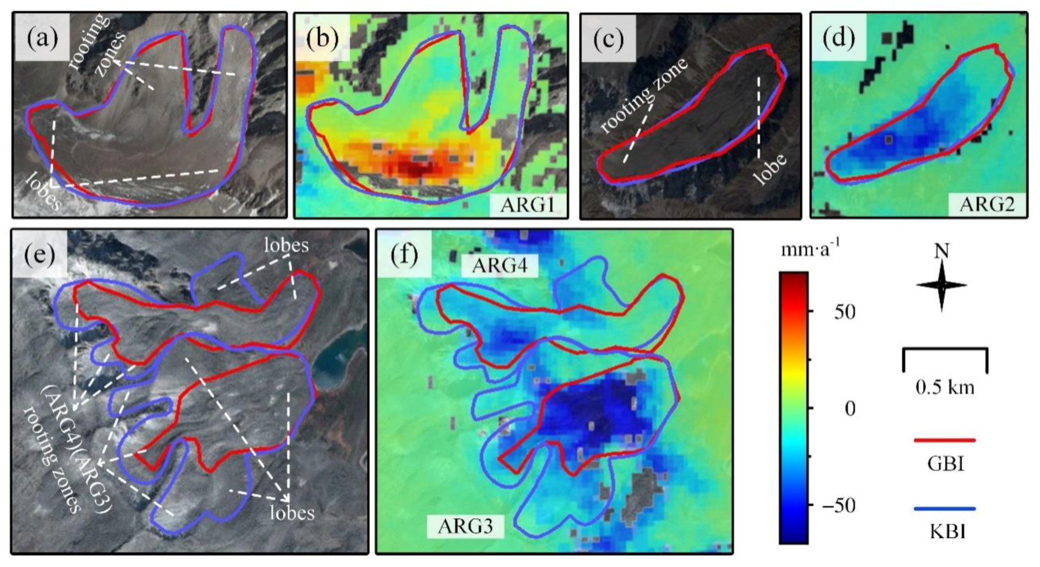
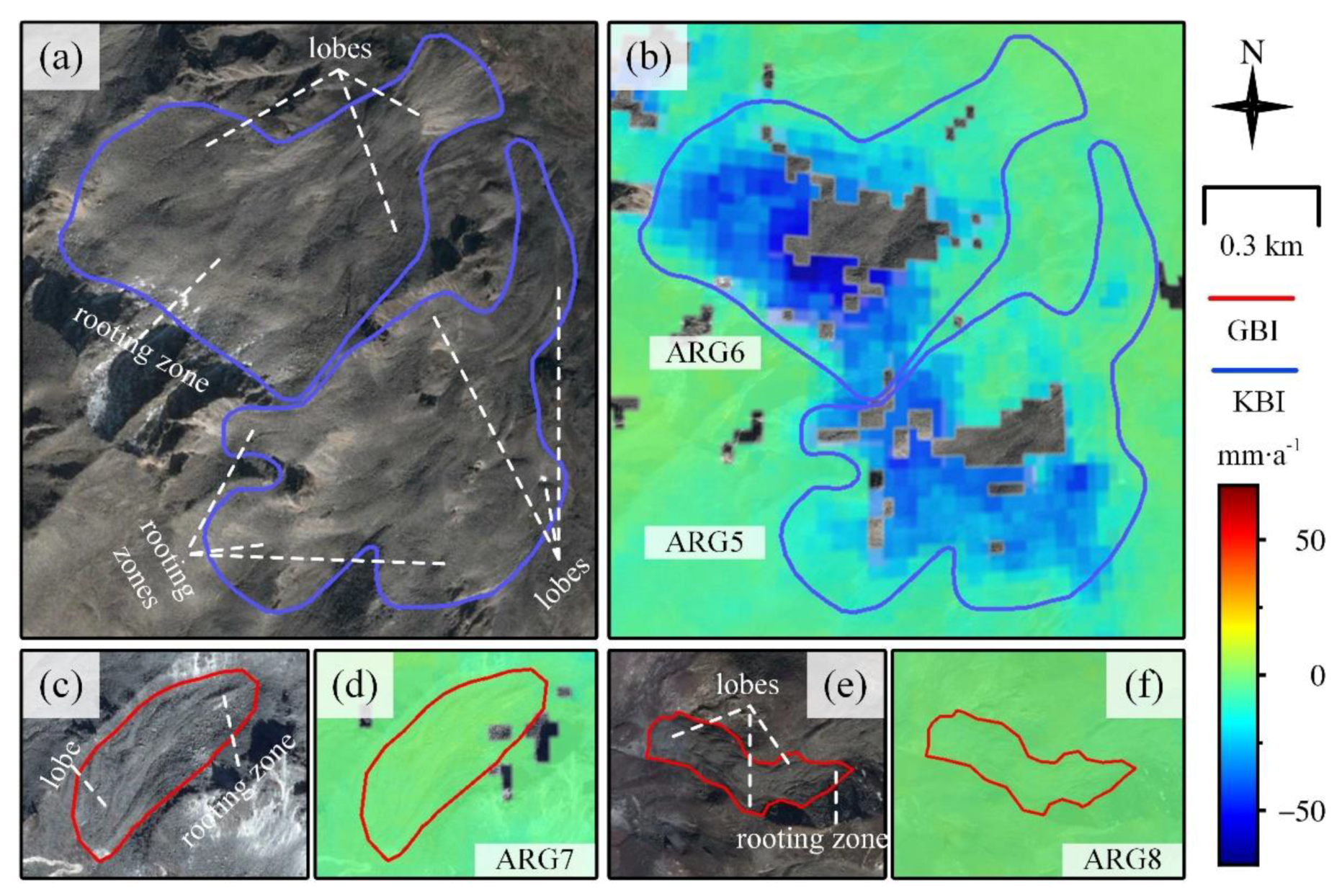
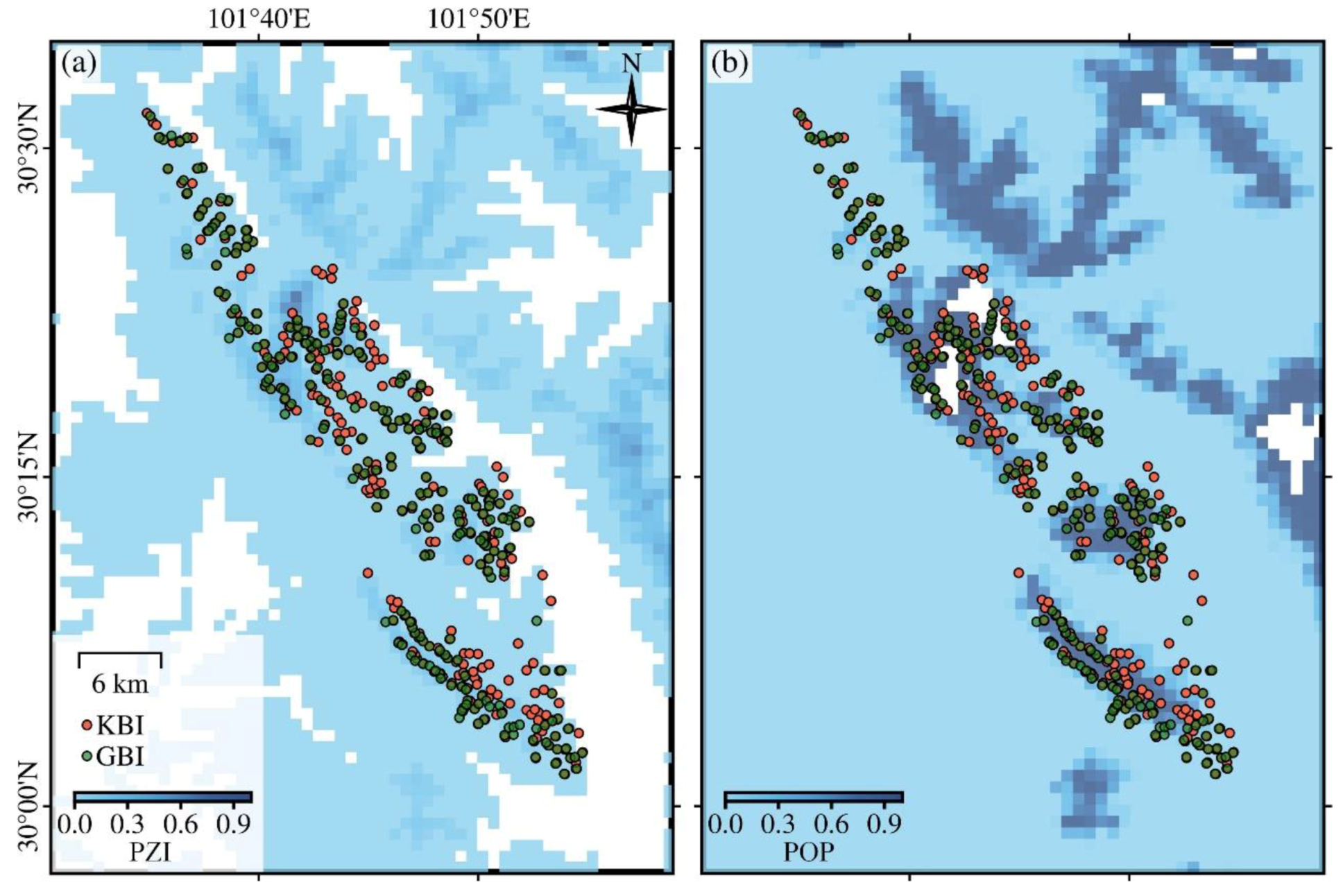
4.2. Comparisons of ARG Distributions and Outlines in KBI and GBI

Two hundred nineteen ARGs were included in both the GBI of Ran and Liu [22] and our InSAR-assist KBI. We found that 149 ARGs from KBI and GBI (accounting for 43% of KBI and 60% of GBI, respectively) were mapped with common boundaries. Figure 5a–d shows the examples of two ARGs sharing common boundaries. The ARG1 in Figure 5a,b is a composite ARG, and the sediment is supplied from two hillslopes. The ARG2 in Figure 5c,d is a typical tongue-shaped ARG, consisting of one rooting zone and one lobe. All the rooting zones and lobes of these two ARGs were mapped in both of the two inventories, with area differences less than 20%.
We found 70 ARGs (accounting for 20% of KBI and 28% of GBI) having different outlines. Figure 5e,f shows two adjacent ARGs as examples that have different outlines in the two inventories. The sediments at both ARGs are supplied from multiple headwalls and transferred into multiple lobes. Two rooting zones and two lobes of the ARG3 were excluded in the GBI. All the rooting zones of ARG4 were partially mapped, with one lobe excluded in the GBI. The areas of ARG3 and ARG4 mapped in KBI are 51% and 29% larger than those from the GBI. It can be seen that, for these complex situations as illustrated above, accurate delineation of the ARG outlines is challenging by only interpreting the geomorphic features. The uncertainties of outlining can be reduced to a large extent by using the InSAR-assist kinematic approach.
The InSAR-assist KBI newly identified 125 ARGs (accounting for 36% of the total number of KBI). Figure 6a,b shows two examples of the newly identified ARGs. The geomorphic features indicating permafrost-related creeping of ARG5 and ARG6 are unclear, making them difficult to distinguish from the surrounding ground in the optical image (Figure 6a). In contrast, evident moving signals of these two ARGs are presented in the multi-temporal InSAR displacement velocity map (Figure 6b).
Thirty-two ARGs were included in GBI but not identified in KBI (accounting for 13% of GBI). We found that about half of these ARGs (15) have aspects of the near north–south direction, indicating that these ARGs are omitted probably because the InSAR measurement is not sensitive to the ground movements in this direction. As an example, Figure 6c,d shows an ARG7 mainly flowing toward the SAR flight azimuth direction (i.e., near north–south direction), while little deformation signal is observed in the InSAR displacement velocity map. We also found 17 ARGs that do not creep along the north–south direction but show geomorphic evidence of permafrost-related creeping (see ARG8 Figure 6e,f as an example). This indicates that the InSAR-assist KBI also has its limitations, which are discussed in Section 5.1.

4.3. Comparative Analysis of the Geomorphic Parameters in GBI and KBI

Table 1 shows the overall statistics of the GBI and KBI. The largest ARGs in GBI and KBI have areas of 1.012 and 0.92 km2, respectively. The ARGs in KBI are generally shorter and steeper in slope than the GBI. The ARGs in KBI and GBI have similar altitude distributions, with the former showing an altitude range of 3860–5094 m a.s.l., and the latter showing a distribution range of 3823–5095 m a.s.l. The total area of the ARGs in KBI is 24% larger than that of the GBI. Next, we show in detail the differences in the geomorphic parameters between GBI and KBI.

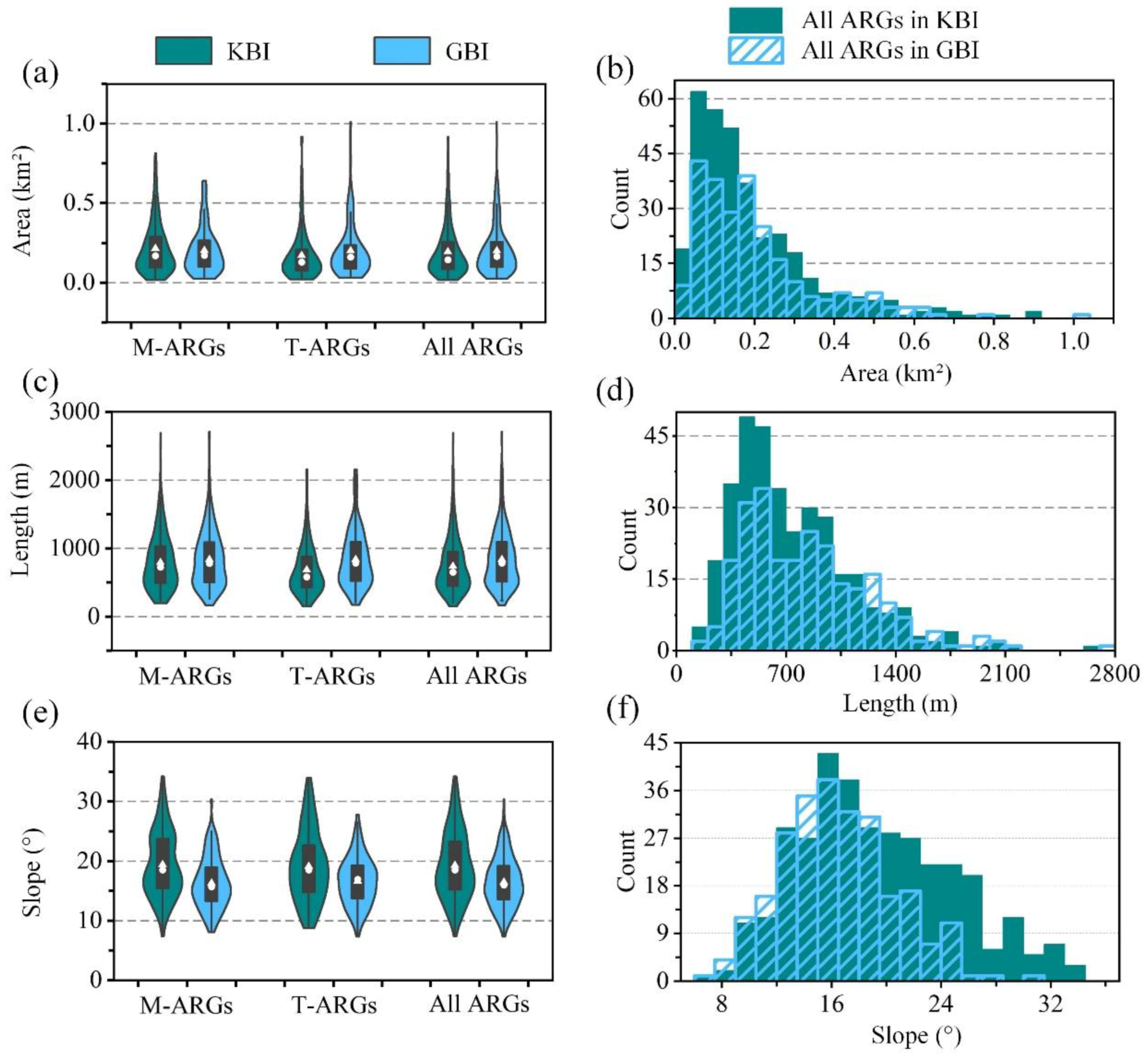
4.3.1. Area, Length, and Slope Angle

The total area of ARGs in KBI is 66.6 km2, among which the moraine type accounts for 58% (38.7 km2), and the talus type accounts for 42% (27.9 km2). In contrast, the total area of ARGs in GBI is 50.6 km2, among which the moraine type accounts for 53% (26.9 km2), and the talus type accounts for 47% (23.8 km2) (Table 1). The mean area of all the ARGs from GBI is 0.2, slightly higher than that from KBI (0.19). Most of the ARGs in both KBI and GBI have areas less than 0.3 km2 (Figure 7a,b).
The mean length of the moraine-type, talus-type, and all ARGs in GBI are 839, 840, and 839 m, overall longer than those of KBI (792, 682, and 736 m, respectively) (Table 1); 62% and 60% of the ARGs in KBI and GBI have lengths ranging from 400 to 1000 m (Figure 7c,d).
Figure 7e,f shows that the ARGs from GBI generally have gentler slopes than those from the KBI. Additionally, the slopes of ARGs from KBI are more widely distributed than GBI. The slopes of ARGs in KBI mainly range between 13° and 25°, while the slopes in GBI mainly range between 11° and 20° (Figure 7e). Particularly, the ARGs newly identified in KBI mostly have slopes higher than 20°, probably because the steep terrain hinders correct interpretations of the geomorphic features and leads to the omissions of ARGs in GBI.

4.3.2. ILP and FLP Altitudes
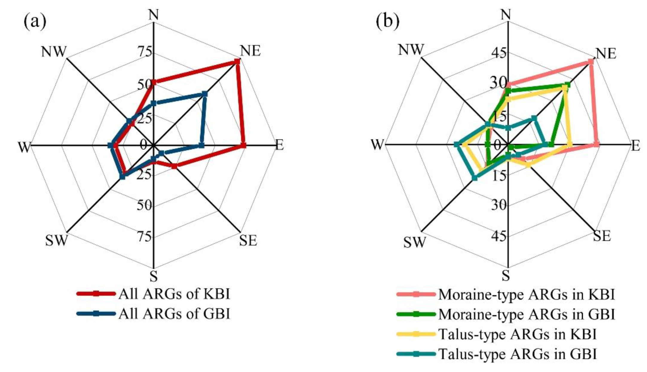
Figure 8 shows the violin plots and histograms of the ILP and FLP altitudes for the two inventories. Both ILP altitudes and FLP altitudes in KBI and GBI show similar distributions. The mean altitudes of ILPs for the moraine-type, talus-type, and all ARGs in KBI are 4628, 4544, and 4588 m, while these values for the GBI are 4612, 4573, and 4593 m. The mean altitudes of FLPs for the moraine-type, talus-type, and all ARGs in KBI are 4376, 4332, and 4355 m, while the corresponding values for the GBI are 4379, 4334, and 4357 m.
The distribution ranges of ILP altitudes of talus-type ARGs are obviously larger than that of the moraine-type ARGs in both inventories, indicating that moraine-type ARGs are generally distributed in a narrow altitudinal range (Figure 8a,c). This is probably because moraine-type ARGs are generally developed from ablated glaciers or interact with glaciers and ice patches within a confined altitude range. We can also observe that the talus-type ARGs reach lower altitudes than moraine-type ARGs in KBI, while this pattern is not obvious in GBI (Figure 8c).

4.3.3. Aspect Angle

Both the GBI and KBI have the most significant number of ARGs (respectively accounting for 24% and 28%) facing the northeast, indicating the northeast slopes are favorable for the ARG formation in Daxue Shan. Except for the aggregated distribution in the northeast direction of GBI, a small amount of ARGs in the GBI face the south (4%) and southeast (4%), and the number of ARGs facing the other directions are nearly equal (11–15% in each direction). In KBI, ARGs show aggregated distribution in the northeast direction (28%), east direction (21%), and north direction (15%), and are also almost evenly distributed in the other directions (7–9% in each direction) (Figure 9a). The significant NE-weighted distribution of ARGs likely results from the topographic control of the Daxue Shan. Previous studies have shown that the slopes receiving lower solar radiation generally favor the presence of ARGs because this helps to preserve ground ice inside ARGs [34]. Given the strike angle of near NW15° for the Daxue Shan mountain ridge, the slopes facing northeast are thus the favorable slopes for forming ARGs.
The moraine-type ARGs in both KBI and GBI show similar aspect distribution patterns (Figure 9b), while the talus-type ARGs in the two inventories show different distributions. Seventy-six percent of the talus-type ARGs in KBI face the north, northeast, and east, whereas only 37% of the talus-type ARGs in GBI face these directions.

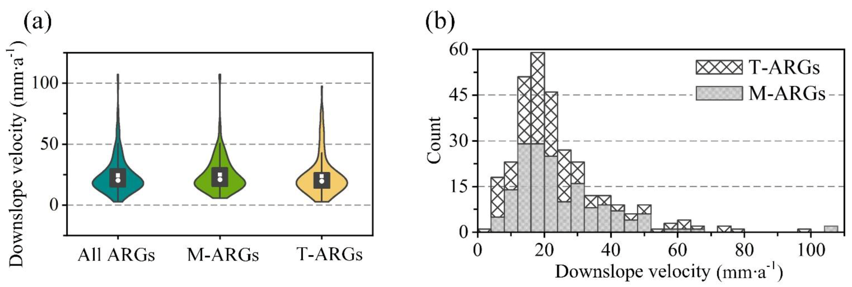
4.4. Active Rock Glacier Velocities

Compared to GBI, the most prominent advantage of KBI is that it can quantify the surface motions of ARGs directly. We calculated the mean downslope movement velocities of 312 ARGs (including 167 moraine-type ARGs and 145 talus-type ARGs) following Equation (1). The velocities of the other 32 ARGs were not documented because their low LOS-to-downslope conversion coefficient may introduce large uncertainties (see Section 3.2). The downslope movement velocities of ARGs in Daxue Shan show high spatial heterogeneity. The mean annual velocities of ARGs range from 2.8 to 107.4 mm∙a−1, with a mean velocity of about 25 mm∙a−1 for all the ARGs (Table 2). The mean movement velocity of moraine-type ARGs (25 mm∙a−1) is slightly higher than that of talus-type ARGs (23.7 mm∙a−1) (Table 2).
Figure 10 shows the violin plot and histogram distribution of the downslope movement velocities for the mapped ARGs. Most velocities concentrate between 10 and 35 mm∙a−1 (Figure 10a). The velocities for both moraine-type and talus-type ARGs mainly range between 10 and 50 mm∙a−1. Only two ARGs have creeping speeds higher than 100 mm∙a−1, and both are moraine-type. The velocity range of ARGs in Daxue Shan is comparable to that in the Uinta Mountains reported by Brencher, Handwerger and Munroe [36]. However, the velocity range is lower than other alpine regions in the Alps, Sierra Nevada, and Northern Tienshan [26,31,34,35].

5. Discussion

5.1. The Geomorphic-Based and Kinematic-Based ARG Inventory Approaches

The geomorphic-based approach can compile exhaustive rock glaciers, including moving and non-moving ones, by visual interpretation of aerial images [9], without tedious data processing. Rock glaciers from GBI have been frequently used to infer the linkages between rock glacier distributions and regional environment variables, e.g., [13,22,45]. However, the completeness of rock glacier mapping and the correctness of its activity classification through the geomorphic-based approach highly depend on the image quality and expertise of the operssator, hence always leading to somewhat subjective mapping results [4]. For example, 36% of ARGs identified by the InSAR-assist kinematic-based approach were failed to be included in GBI in Daxue Shan. Additionally, 29% of ARGs from GBI were mapped incompatibly with respect to their kinematic boundaries. These variabilities in mapping outcomes can propagate to the subsequent geomorphic parameter calculations, and even induce large uncertainties in the further cryosphere-related studies relying on rock glaciers
Compared to the geomorphic-based approach, the kinematic-based approach can help effectively detect and accurately delineate ARGs. The kinematic-based approach can also quantify the surface motions of ARGs. This approach is thus relatively more objective and can reduce the uncertainties in future studies based on the identified ARGs [46]. We here suggest using multi-annual mean displacement signals to detect moving targets firstly, and then systematically integrating the kinematic features and geomorphic characteristics to identify and map rock glaciers.
Our study in Daxue Shan demonstrates that the InSAR-assist kinematic-based approach also has its own limitations. First, the ARGs facing the satellite flight direction may be missed by this approach because of the insensitivity of InSAR measurement to ground movement along this direction. In our study region, 15 ARGs facing the near north–south direction (accounting for 6% of GBI) failed to be detected by InSAR, although all of them exhibit clear geomorphic features indicating permafrost-related creeping. Second, shadow and layover distortions in SAR images can degrade the displacement signal and lead to some of the ARGs being omitted in the inventory. Some researchers only included ARGs located outside layover and shadow zones in the ARG inventories [31]. The SAR images used in this study have about 5.9% pixels affected by overlay and shadow effects, implying that these SAR geometric distortions have limited influences on the inventory results. However, for regions with rugged topography where SAR images may be strongly affected by shadow and layover, it is suggested to use SAR images acquired from different orbits (e.g., ascending and descending) to conduct the inventory. In addition, SAR signal decorrelation due to the alpine environment changes and atmospheric delays is also the common error source in InSAR displacement measurements, which may influence the completeness and correctness of the kinematic-based rock glacier inventory.
Future ARG inventories should value the integration of both geomorphic and kinematic features of ARGs using advanced methods such as machine learning or deep learning algorithms. These advanced methods can automatically recognize recurring patterns and textures and thus reduce the workload in compiling rock glaciers. Furthermore, recent studies have shown that machine learning-based SAR data processing can better identify and correct the artifacts in surface displacement measurement [47]. We suggest that developing machine learning-based methods for extracting both geomorphic and kinematic information of rock glaciers is a possible solution to homogeneous compilation and global assemblage of rock glacier inventories.

5.2. Influences of SAR Image Selection on ARG Inventory

We discussed the advantages and limitations of InSAR-assist ARG mapping in Section 5.1. Besides using multi-temporal SAR images, as shown in this study, using a signal SAR image pair has also been frequently applied to map ARGs. Additionally, considering that the downslope movements of ARGs generally show a seasonal fluctuation pattern, we postulate that using SAR images acquired in different seasons may also influence the inventory. Here, we discuss the reasonable strategy of SAR data processing aimed at overcoming the limitations of InSAR for ARG inventory.

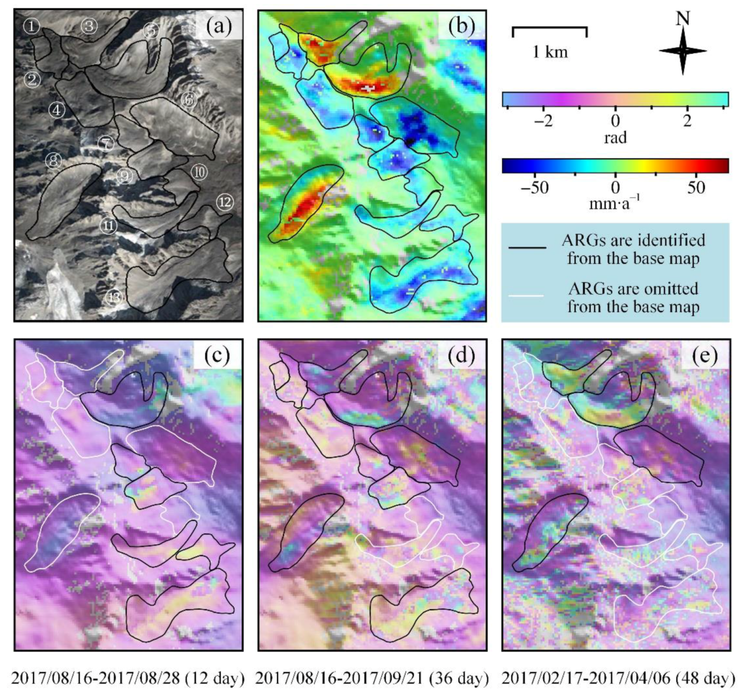
5.2.1. Active Rock Glacier Inventory from a Single SAR Image Pair

The use of only one or a few SAR interferograms to detect ARGs has been successfully implemented in the Sierra Nevada [31], Tien Shan [34], and Dry Andes Mountains [48], etc., where 59, 261, and 2116 ARGs have been mapped, respectively. However, the effectiveness of this strategy is closely related to the quality of the SAR interferogram. Given that ARGs creep with diverse velocities, SAR interferograms should be carefully selected with proper temporal baselines. For instance, ground displacements in the range 8–90 cm a−1 can be measured from a Sentinel-1 SAR interferogram with 12 day temporal baseline, while the displacement range will be reduced to 2–30 cm a−1 when the temporal baseline extends to one month [49]. The simple calculations imply that slowing ARGs may be missed by using a SAR interferogram with a temporal baseline that is too short because the ARGs cannot be distinguished from the stable surrounding ground. On the other hand, if the temporal baseline is too long, SAR temporal decorrelation may, in turn, cause unsuccessful measurement of the displacement signals. Selecting the SAR image pair with an appropriate temporal baseline is thus crucial for single SAR interferogram-based ARG inventorying.
To demonstrate the influence of interferogram time span on the variability of ARG mapping, we selected a region (see the location in Figure 4b) containing 11 ARGs and then examined the ARG numbers identified from three SAR interferograms with 12-, 36-, and 48-day temporal baselines (Figure 11c–e). We can identify 6, 10, and 4 ARGs (the black polygons) from the 12-, 36-, and 38-day temporal-span interferograms, respectively. For example, the ARG No. 3 (Figure 11a) cannot be identified in the 12-day-span interferogram, but show some movement signals in the 36- and 48-day-span interferogram. Additionally, ARG No. 10 cannot be identified in all three interferograms, but can be clearly detected in the multi-temporal InSAR mean velocity map (Figure 11b). This indicates that using a single SAR interferogram for ARG inventory could lead to a high omission rate.
When only using one image pair to inventory ARGs, to improve the compilation completeness, it is suggested to use SAR images acquired by the SAR sensor emitting long radar wavelengths, such as the L-band ALOS PALSAR. Long radar wavelength generally has a good penetration ability and thus can preserve SAR coherence for measurement accuracy [26,31,34]. Nevertheless, our study in Daxue Shan suggests that using multi-temporal InSAR is a better option than using only one single SAR image pair for ARGs inventorying. Surface displacement velocity maps derived from the advanced InSAR algorithms can provide better kinematic information of ARGs and ensure completeness and accuracy of the inventory.

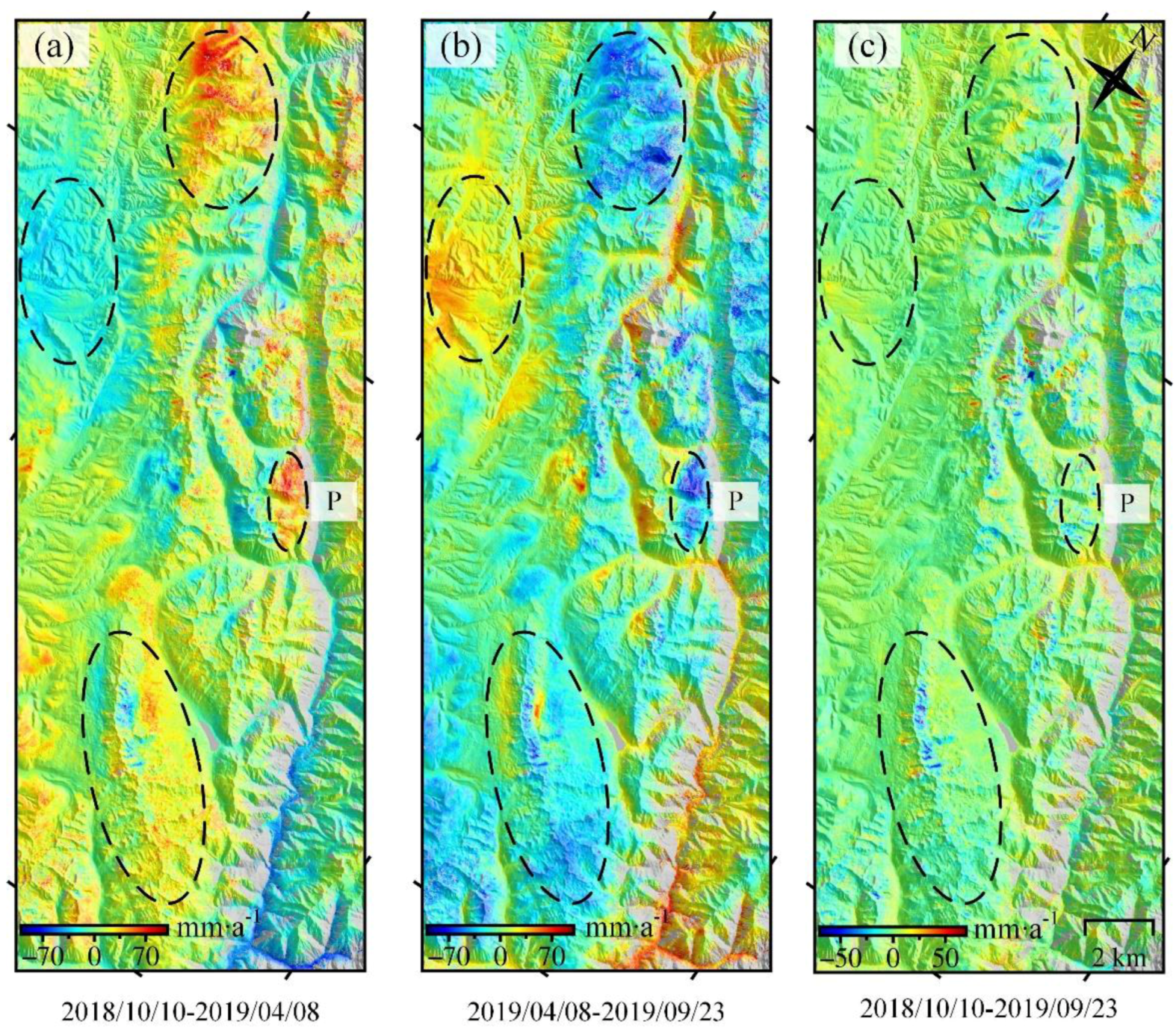
5.2.2. Influence of SAR Acquisition Season on ARG Inventories

The winter season in Daxue Shan is defined from October to March of the following year, and the summer season is defined from April to September within a year. To infer the influence of SAR acquisition season on ARG inventories, we derived the surface displacement velocities using images only acquired either in the winter (Figure 12a) or summer (Figure 12b) season, respectively. As a comparison, Figure 12c shows the velocity map using all the SAR images.
Both the winter and summer surface velocities are different from the full-data-derived velocities, especially in the mountain ridges and valleys (see the polygons in Figure 12). We randomly selected an area P as an example and compared the displacements for this region in the three velocity maps. The velocity values are positive for area P in the winter velocity map representing displacements toward the satellite in the LOS direction (Figure 12a). However, the velocity values become negative in the summer velocity map (Figure 12b). Widespread homogenous “displacement signals” can be found in the area P either in the winter or summer seasons, preventing us from identifying the moving ground targets. This indicates that using the ground deformation products generated from only winter or summer SAR images can result in a highly biased inventory. The inverse displacement signals for the same area between the winter and summer velocity map probably result from seasonal atmospheric delay or hydrological loading effects [50]. In contrast, clear displacement signals associated with ARG creeping can be seen in the velocity map derived from full SAR data (Figure 12c), suggesting that the SAR dataset used for ARG inventories should cover at least one complete cycle year.

5.3. Implication for Rock Glacier-Based Permafrost Distribution Estimation

Rock glaciers have been ubiquitously used in permafrost distribution mapping since they are regarded as the visible indicators of permafrost occurrence. Based on rock glaciers’ activity status (i.e., active or relict), the probability of permafrost occurrence can be linked to the regional environmental variables such as altitude, mean annual air temperature (MMAT), ground temperature, and solar radiation through statistic models. A few studies have relied on the geomorphic-based rock glacier inventories to estimate the permafrost distribution in the Southern Alps, New Zealand [51], Hunza River Basin, Chilean Andes [52], Western Karakoram [53], and Sikkim Himalayas [54].
We compared the ARGs mapped from GBI and KBI with the existing permafrost distribution maps from statistical modeling. Figure 13a,b shows the GBI and KBI superimposed on the Global Permafrost Zonation Index (PZI) map developed by Gruber [55] and Northern Hemisphere Permafrost Occurrence Probability (POP) map developed by Obu, et al. [56]. The PZI map was established by modeling the relationship between long-term mean annual air temperature (MAAT) and permafrost occurrence using the simple but widely accepted cumulative normal distribution [55]. The POP map used the TTOP (temperature at the top of permafrost) equilibrium model to link permafrost occurrence with environment variables, including remotely sensed land surface temperatures and downscaled ERA-Interim climate reanalysis data, tundra wetness classes, and landcover map [57]. Both the PZI and POP values close to 1 indicate high probabilities of permafrost occurrence. Statistics show that the mean PZI values are both smaller than 0.1 for the ARGs from KBI (0.07) and GBI (0.09) in Daxue Shan. The mean POP values for ARGs in KBI and GBI are moderate, with values of 0.48 and 0.46, respectively (Table 3). Among the 344 and 251 ARGs included in KBI and GBI, only 2 and 1 ARGs have PZI values higher than 0.5. The numbers of ARGs showing POP values higher than 0.5 are 164 and 111 for KBI and GBI, respectively.
The KBI and GBI have comparable permafrost statistical indices with slight discrepancy (Table 3), although our results (Section 4) have shown that the ARGs from these two inventories are different in distributions, outlines, and geographic parameters. The similar statistics between PZI and POP of GBI and KBI are probably due to the coarse spatial resolution (both at 1 km2) of PZI and POP maps.
The small to moderate PZI and POP values on the ARGs also indicate that the global permafrost distribution products from statistical modeling significantly underestimated the permafrost extent in the Daxue Shan region. This is probably due to the lack of accurate constraints (i.e., air temperature and precipitation) on the permafrost estimation model. Furthermore, given that solar radiation, topography, and snow depth all have influences on the ground thermal regime [58], which control the occurrence of permafrost, using relatively simple empirical models to estimate large-scale permafrost distribution may somewhat be biased. In addition, ARGs move downslope and may reach the permafrost-free region. Due to the cooling effect of rock glaciers through their high porosity and storage of ice, rock glaciers can lead to a more favorable environment for permafrost occurrence than the surrounding terrain [58,59].

5.4. Implications for Water Storage Content Estimation

Although ARGs are generally smaller than glaciers, they are regarded as long-term reservoirs of great value in hydrology because of their large number and wide distribution. With increasing temperature in the future, ARGs may become increasingly more important freshwater resources in arid and semiarid areas [5]. Rock glaciers compiled from the geomorphic-based approach have been used for water content estimations in several mountain ranges, with assumptions of a certain ice content and ice thickness. For example, based on the 669 rock glaciers from geomorphic-based interpretation, Janke, Ng and Bellisario [17] assumed a rock glacier ice content of about 25–44.9% and estimated water storage of 2200–4858 km3 in the semiarid Aconcagua River Basin of Chile. Similarly, Jones, et al. [60] estimated the water content of rock glaciers at about 1.672 × 10¹⁰–2.508 × 10¹⁰ km3 in Nepalese Himalaya with an assumption of ice content at 40–60% from a GBI including 1137 ARGs. Considering the heterogeneous properties of rock glaciers, apparently, the simple assumptions of ice content and thickness may lead to significantly biased estimates.
Using rock glaciers from KBI may overcome these limitations of GBI for regional water storage content calculations. First, as shown in the Daxue Shan case, the KBI can achieve a more complete compilation of rock glaciers than GBI, with 36% differences in numbers and 24% differences in total areas. Second, the kinematic information can help improve the accuracy of ice content estimates. Several studies have shown that rock glacier downslope movements can be related to their ice content through rheological models [12,61]. The better estimation of ice content can thus improve the water storage content estimates. We suggest that the kinematic-based rock glacier inventories are useful for inferring the hydrological significance of rock glaciers [61].

6. Conclusions

In this study, we compared the kinematic-based and geomorphic-based rock glacier inventory approaches in the Daxue Shan region. We employed the multi-temporal InSAR velocity map and Google Earth optical images to assist the identification of ARGs. Compared to the inventory from the geomorphic-based approach, our InSAR-assist kinematic-based inventory overall shows better completeness and accuracy. We newly identified 125 ARGs in the study region, which is 36% more than the GBI.
We found that 149 ARGs share common outlines and 70 ARGs were mapped with different polygon outlines. Thirty-two ARGs included in GBI were not identified by the InSAR-assist kinematic-based approach (accounting for 11% of GBI), which was mainly caused by the insensitivity of InSAR measurements to ground movements parallel to the satellite motion. The total area of ARGs in KBI is 24% more than that in GBI. The ARGs in GBI are overall longer and distributed on more gentle slopes than those from KBI. Both ILP and FLP altitudes in the two inventories show similar altitudinal distributions. Aspect distribution patterns of GBI and KBI show obvious discrepancies, especially for the talus-type ones. The downslope velocities of ARGs are concentrated in the range 10–35 mm∙a−1, with only 2 ARGs creeping faster than 100 mm∙a−1.
Inventories from InSAR-assist kinematic-based approach may be affected by the season of SAR data acquisition, geometry distortions, the sensitivity of InSAR measurement to ground deformation, and SAR signal decorrelations. Using multi-temporal SAR images spanning at least one year to derive the surface deformation map is an effective way to overcome these limitations. We inferred that the inventory approach greatly influences the additional rock glacier-based studies, such as permafrost distribution mapping and water equivalent estimates. The kinematic-based inventory approach is useful in the future because of its potential in providing complete and accurate ARG inventories and realistic constraints on the inversion of hydrological parameters on ARGs. Advanced methods such as machine learning or deep learning algorithms for automatic identification of both geomorphic and kinematic features of ARGs should also be valued in future inventories.

Author Contributions

Conceptualization, X.W.; data curation, J.C.; funding acquisition, X.W. and G.L.; methodology, J.C.; project administration, X.W.; software, J.C. and X.W.; writing—original draft, J.C.; writing—review and editing, X.W., G.L. and B.Y. All authors have read and agreed to the published version of the manuscript.

Funding

This work was supported by the National Natural Science Foundation of China under Grant No. (41804009, 42071410, 42171355), the Project of Application Foundation of the Sichuan (China) Science and Technology (No. 2020YJ0322, 2020JDTD0003, 2019ZDZX0042), and by the China Scholarship Council.

Institutional Review Board Statement

Not applicable.

Informed Consent Statement

Not applicable.

Data Availability Statement

The active rock glacier datasets from InSAR-assist kinematic-based approach in Daxue Shan, Southeast Tibetan Plateau are available at Plateau https://zenodo.org/record/5607677 (accessed date on 28 October 2021).

Acknowledgments

The authors appreciate ESA and JAXA for the free deliveries of the Sentinel-1 images and AW3D30 DEM data. Zeze Ran and Gengnian Liu are also highly acknowledged for their contributions to the rock glacier inventory in Daxue Shan. The permafrost distribution map made by Defu Zou is available at https://tc.copernicus.org/articles/11/2527/2017/ (accessed date on 28 October 2021); PZI map made by S. Gruber can be downloaded from http://www.geo.uzh.ch/microsite/cryodata (accessed date on 28 October 2021); TTOP map provided by Jaroslav Obu is available at https://doi.pangaea.de/10.1594/PANGAEA.888600 (accessed date on 28 October 2021).

Conflicts of Interest

The authors declare no conflict of interest.

References

  1. Capps, S.R., Jr. Rock glaciers in Alaska. J. Geol. 1910, 18, 359–375. [Google Scholar] [CrossRef]
  2. Ostrem, G. Rock glaciers and ice-cored moraines, a reply to D. Barsch. Geogr. Ann. Ser. A Phys. Geogr. 1971, 53, 207–213. [Google Scholar] [CrossRef]
  3. Barsch, D. Active rock glaciers as indicators for discontinuous alpine permafrost. An example from the Swiss Alps. In Proceedings of the International Conference on Permafrost, Edmonton, AB, Canada, 10–13 July 1978. [Google Scholar]
  4. Brardinoni, F.; Scotti, R.; Sailer, R.; Mair, V. Evaluating sources of uncertainty and variability in rock glacier inventories. Earth Surf. Process. Landf. 2019, 44, 2450–2466. [Google Scholar] [CrossRef]
  5. Azócar, G.F.; Brenning, A. Hydrological and geomorphological significance of rock glaciers in the dry Andes, Chile (27°–33° S). Permafr. Periglac. Process. 2010, 21, 42–53. [Google Scholar] [CrossRef]
  6. Jones, D.B.; Harrison, S.; Anderson, K.; Whalley, W.B. Rock glaciers and mountain hydrology: A review. Earth Sci. Rev. 2019, 193, 66–90. [Google Scholar] [CrossRef]
  7. Brenning, A. Geomorphological, hydrological and climatic significance of rock glaciers in the Andes of Central Chile (33–35° S). Permafr. Periglac. Process. 2005, 16, 231–240. [Google Scholar] [CrossRef]
  8. Knight, J.; Harrison, S.; Jones, D.B. Rock glaciers and the geomorphological evolution of deglacierizing mountains. Geomorphology 2019, 324, 14–24. [Google Scholar] [CrossRef]
  9. Delaloye, R.; Barboux, C.; Bodin, X.; Brenning, A.; Hartl, L.; Hu, Y.; Ikeda, A.; Kaufmann, V.; Kellerer-Pirklbauer, A.; Lambiel, C. Rock glacier inventories and kinematics: A new IPA Action Group. In Proceedings of the 5th European Conference on Permafrost, Chamonix-Mont Blanc, France, 23 June–1 July 2018; pp. 392–393. [Google Scholar]
  10. Hu, Y.; Liu, L.; Wang, X.; Zhao, L.; Wu, T.; Cai, J.; Zhu, X.; Hao, J. Quantification of permafrost creep provides kinematic evidence for classifying a puzzling periglacial landform. Earth Surf. Process. Landf. 2020, 46, 465–477. [Google Scholar] [CrossRef]
  11. Marcer, M.; Serrano, C.; Brenning, A.; Bodin, X.; Goetz, J.; Schoeneich, P. Evaluating the destabilization susceptibility of active rock glaciers in the French Alps. Cryosphere 2019, 13, 141–155. [Google Scholar] [CrossRef] [Green Version]
  12. Cicoira, A.; Beutel, J.; Faillettaz, J.; Gärtner-Roer, I.; Vieli, A. Resolving the influence of temperature forcing through heat conduction on rock glacier dynamics: A numerical modelling approach. Cryosphere 2019, 13, 927–942. [Google Scholar] [CrossRef] [Green Version]
  13. Onaca, A.; Ardelean, F.; Urdea, P.; Magori, B. Southern Carpathian rock glaciers: Inventory, distribution and environmental controlling factors. Geomorphology 2017, 293, 391–404. [Google Scholar] [CrossRef]
  14. Onaca, A.L.; Urdea, P.; Ardelean, A.C. Internal structure and permafrost characteristics of the rock glaciers of southern carpathians (Romania) assessed by geoelectrical soundings and thermal monitoring. Geogr. Ann. Ser. A Phys. Geogr. 2016, 95, 249–266. [Google Scholar] [CrossRef]
  15. Berthling, I. Beyond confusion: Rock glaciers as cryo-conditioned landforms. Geomorphology 2011, 131, 98–106. [Google Scholar] [CrossRef]
  16. Cao, B.; Li, X.; Feng, M.; Zheng, D. Quantifying Overestimated Permafrost Extent Driven by Rock Glacier Inventory. Geophys. Res. Lett. 2021, 48, e2021GL092476. [Google Scholar] [CrossRef]
  17. Janke, J.R.; Ng, S.; Bellisario, A. An inventory and estimate of water stored in firn fields, glaciers, debris-covered glaciers, and rock glaciers in the Aconcagua River Basin, Chile. Geomorphology 2017, 296, 142–152. [Google Scholar] [CrossRef]
  18. Esper Angillieri, M.Y. A preliminary inventory of rock glaciers at 30° S latitude, Cordillera Frontal of San Juan, Argentina. Quat. Int. 2009, 195, 151–157. [Google Scholar] [CrossRef]
  19. Brenning, A.; Long, S.; Fieguth, P. Detecting rock glacier flow structures using Gabor filters and IKONOS imagery. Remote Sens. Environ. 2012, 125, 227–237. [Google Scholar] [CrossRef]
  20. Scotti, R.; Brardinoni, F.; Alberti, S.; Frattini, P.; Crosta, G.B. A regional inventory of rock glaciers and protalus ramparts in the central Italian Alps. Geomorphology 2013, 186, 136–149. [Google Scholar] [CrossRef]
  21. Schmid, M.O.; Baral, P.; Gruber, S.; Shahi, S.; Shrestha, T.; Stumm, D.; Wester, P. Assessment of permafrost distribution maps in the Hindu Kush Himalayan region using rock glaciers mapped in Google Earth. Cryosphere 2015, 9, 2089–2099. [Google Scholar] [CrossRef] [Green Version]
  22. Ran, Z.; Liu, G. Rock glaciers in Daxue Shan, south-eastern Tibetan Plateau: An inventory, their distribution, and their environmental controls. Cryosphere 2018, 12, 2327–2340. [Google Scholar] [CrossRef] [Green Version]
  23. Marcer, M. Rock glaciers automatic mapping using optical imagery and convolutional neural networks. Permafr. Periglac. Process. 2020, 31, 561–566. [Google Scholar] [CrossRef]
  24. Brenning, A. Benchmarking classifiers to optimally integrate terrain analysis and multispectral remote sensing in automatic rock glacier detection. Remote Sens. Environ. 2009, 113, 239–247. [Google Scholar] [CrossRef]
  25. Robson, B.A.; Bolch, T.; MacDonell, S.; Hölbling, D.; Rastner, P.; Schaffer, N. Automated detection of rock glaciers using deep learning and object-based image analysis. Remote Sens. Environ. 2020, 250, 112033. [Google Scholar] [CrossRef]
  26. Kääb, A.; Strozzi, T.; Bolch, T.; Caduff, R.; Trefall, H.; Stoffel, M.; Kokarev, A. Inventory, motion and acceleration of rock glaciers in Ile Alatau and Kungöy Ala-Too, northern Tien Shan, since the 1950s. Cryosphere Discuss. 2020, 2020, 1–37. [Google Scholar] [CrossRef]
  27. Ulrich, V.; Williams, J.G.; Zahs, V.; Anders, K.; Hecht, S.; Höfle, B. Measurement of rock glacier surface change over different timescales using terrestrial laser scanning point clouds. Earth Surf. Dyn. 2021, 9, 19–28. [Google Scholar] [CrossRef]
  28. Massonnet, D.; Feigl, K.L. Radar interferometry and its application to changes in the Earth’s surface. Rev. Geophys. 1998, 36, 441–500. [Google Scholar] [CrossRef] [Green Version]
  29. Nagler, T.; Mayer, C.; Rott, H. Feasibility of DINSAR for mapping complex motion fields of Alpine ice-and rock-glaciers. In Proceedings of the Third International Symposium on Retrieval of Bio-and Geo-Physical Parameters from SAR Data for Land Applications, Sheffield, UK, 11–14 September 2002; pp. 377–382. [Google Scholar]
  30. Lilleøren, K.S.; Etzelmüller, B.; Gärtner-Roer, I.; Kääb, A.; Westermann, S.; Gudmundsson, A. The Distribution, Thermal Characteristics and Dynamics of Permafrost in Tröllaskagi, Northern Iceland, as Inferred from the Distribution of Rock Glaciers and Ice-Cored Moraines. Permafr. Periglac. Process. 2013, 24, 322–335. [Google Scholar] [CrossRef]
  31. Liu, L.; Millar, C.I.; Westfall, R.D.; Zebker, H.A. Surface motion of active rock glaciers in the Sierra Nevada, California, USA: Inventory and a case study using InSAR. Cryosphere 2013, 7, 1109–1119. [Google Scholar] [CrossRef] [Green Version]
  32. Barboux, C.; Delaloye, R.; Lambiel, C. Inventorying slope movements in an Alpine environment using DInSAR. Earth Surf. Process. Landf. 2014, 39, 2087–2099. [Google Scholar] [CrossRef] [Green Version]
  33. Necsoiu, M.; Onaca, A.; Wigginton, S.; Urdea, P. Rock glacier dynamics in Southern Carpathian Mountains from high-resolution optical and multi-temporal SAR satellite imagery. Remote Sens. Environ. 2016, 177, 21–36. [Google Scholar] [CrossRef] [Green Version]
  34. Wang, X.; Liu, L.; Zhao, L.; Wu, T.; Li, Z.; Liu, G. Mapping and inventorying active rock glaciers in the northern Tien Shan of China using satellite SAR interferometry. Cryosphere 2017, 11, 997–1014. [Google Scholar] [CrossRef] [Green Version]
  35. Strozzi, T.; Caduff, R.; Jones, N.; Barboux, C.; Delaloye, R.; Bodin, X.; Kääb, A.; Mätzler, E.; Schrott, L. Monitoring Rock Glacier Kinematics with Satellite Synthetic Aperture Radar. Remote Sens. 2020, 12, 559. [Google Scholar] [CrossRef] [Green Version]
  36. Brencher, G.; Handwerger, A.L.; Munroe, J.S. InSAR-based characterization of rock glacier movement in the Uinta Mountains, Utah, USA. Cryosphere 2021, 15, 4823–4844. [Google Scholar] [CrossRef]
  37. Reinosch, E.; Gerke, M.; Riedel, B.; Schwalb, A.; Ye, Q.; Buckel, J. Rock glacier inventory of the western Nyainqêntanglha Range, Tibetan Plateau, supported by InSAR time series and automated classification. Permafr. Periglac. Process. 2021, 32, 657–672. [Google Scholar] [CrossRef]
  38. Zou, D.; Zhao, L.; Sheng, Y.; Chen, J.; Hu, G.; Wu, T.; Wu, J.; Xie, C.; Wu, X.; Pang, Q.; et al. A new map of permafrost distribution on the Tibetan Plateau. Cryosphere 2017, 11, 2527–2542. [Google Scholar] [CrossRef] [Green Version]
  39. Zhang, P.-Z. A review on active tectonics and deep crustal processes of the Western Sichuan region, eastern margin of the Tibetan Plateau. Tectonophysics 2013, 584, 7–22. [Google Scholar] [CrossRef]
  40. Ferretti, A.; Fumagalli, A.; Novali, F.; Prati, C.; Rocca, F.; Rucci, A. A New Algorithm for Processing Interferometric Data-Stacks: SqueeSAR. IEEE Trans. Geosci. Remote Sens. 2011, 49, 3460–3470. [Google Scholar] [CrossRef]
  41. Wegnüller, U.; Werner, C.; Strozzi, T.; Wiesmann, A.; Frey, O.; Santoro, M. Sentinel-1 Support in the GAMMA Software. Procedia Comput. Sci. 2016, 100, 1305–1312. [Google Scholar] [CrossRef] [Green Version]
  42. Tadono, T.; Nagai, H.; Ishida, H.; Oda, F.; Naito, S.; Minakawa, K.; Iwamoto, H. Generation of the 30 M-Mesh Global Digital Surface Model by Alos Prism. ISPRS Int. Arch. Photogramm. Remote Sens. Spat. Inf. Sci. 2016, XLI-B4, 157–162. [Google Scholar] [CrossRef] [Green Version]
  43. Yunjun, Z.; Fattahi, H.; Amelung, F. Small baseline InSAR time series analysis: Unwrapping error correction and noise reduction. Comput. Geosci. 2019, 133, 104331. [Google Scholar] [CrossRef] [Green Version]
  44. Jolivet, R.; Grandin, R.; Lasserre, C.; Doin, M.P.; Peltzer, G. Systematic InSAR tropospheric phase delay corrections from global meteorological reanalysis data. Geophys. Res. Lett. 2011, 38. [Google Scholar] [CrossRef] [Green Version]
  45. Rangecroft, S.; Harrison, S.; Anderson, K.; Magrath, J.; Castel, A.P.; Pacheco, P. A First Rock Glacier Inventory for the Bolivian Andes. Permafr. Periglac. Process. 2014, 25, 333–343. [Google Scholar] [CrossRef]
  46. Roer, I.; Nyenhuis, M. Rockglacier activity studies on a regional scale: Comparison of geomorphological mapping and photogrammetric monitoring. Earth Surf. Process. Landf. 2007, 32, 1747–1758. [Google Scholar] [CrossRef]
  47. Rouet-Leduc, B.; Jolivet, R.; Dalaison, M.; Johnson, P.A.; Hulbert, C. Autonomous extraction of millimeter-scale deformation in InSAR time series using deep learning. Nat. Commun. 2021, 12, 6480. [Google Scholar] [CrossRef]
  48. Villarroel, C.; Tamburini Beliveau, G.; Forte, A.; Monserrat, O.; Morvillo, M. DInSAR for a Regional Inventory of Active Rock Glaciers in the Dry Andes Mountains of Argentina and Chile with Sentinel-1 Data. Remote Sens. 2018, 10, 1588. [Google Scholar] [CrossRef] [Green Version]
  49. Torres, R.; Snoeij, P.; Geudtner, D.; Bibby, D.; Davidson, M.; Attema, E.; Potin, P.; Rommen, B.; Floury, N.; Brown, M. GMES Sentinel-1 mission. Remote Sens. Environ. 2012, 120, 9–24. [Google Scholar] [CrossRef]
  50. Rouyet, L.; Lauknes, T.R.; Christiansen, H.H.; Strand, S.M.; Larsen, Y. Seasonal dynamics of a permafrost landscape, Adventdalen, Svalbard, investigated by InSAR. Remote Sens. Environ. 2019, 231, 111236. [Google Scholar] [CrossRef]
  51. Sattler, K.; Anderson, B.; Mackintosh, A.; Norton, K.; de Róiste, M. Estimating Permafrost Distribution in the Maritime Southern Alps, New Zealand, Based on Climatic Conditions at Rock Glacier Sites. Front. Earth Sci. 2016, 4, 4. [Google Scholar] [CrossRef] [Green Version]
  52. Azócar, G.F.; Brenning, A.; Bodin, X. Permafrost distribution modelling in the semi-arid Chilean Andes. Cryosphere 2017, 11, 877–890. [Google Scholar] [CrossRef] [Green Version]
  53. Hassan, J.; Chen, X.; Muhammad, S.; Bazai, N.A. Rock glacier inventory, permafrost probability distribution modeling and associated hazards in the Hunza River Basin, Western Karakoram, Pakistan. Sci. Total Environ. 2021, 782, 146833. [Google Scholar] [CrossRef] [PubMed]
  54. Haq, M.A.; Baral, P. Study of permafrost distribution in Sikkim Himalayas using Sentinel-2 satellite images and logistic regression modelling. Geomorphology 2019, 333, 123–136. [Google Scholar] [CrossRef]
  55. Gruber, S. Derivation and analysis of a high-resolution estimate of global permafrost zonation. Cryosphere 2012, 6, 221–233. [Google Scholar] [CrossRef] [Green Version]
  56. Obu, J.; Westermann, S.; Bartsch, A.; Berdnikov, N.; Christiansen, H.H.; Dashtseren, A.; Delaloye, R.; Elberling, B.; Etzelmüller, B.; Kholodov, A.; et al. Northern Hemisphere permafrost map based on TTOP modelling for 2000–2016 at 1 km2 scale. Earth Sci. Rev. 2019, 193, 299–316. [Google Scholar] [CrossRef]
  57. Smith, M.; Riseborough, D. Permafrost monitoring and detection of climate change. Permafr. Periglac. Process. 1996, 7, 301–309. [Google Scholar] [CrossRef]
  58. Harrington, J.S.; Hayashi, M. Application of distributed temperature sensing for mountain permafrost mapping. Permafr. Periglac. Process. 2019, 30, 113–120. [Google Scholar] [CrossRef]
  59. Gubler, S.; Fiddes, J.; Keller, M.; Gruber, S. Scale-dependent measurement and analysis of ground surface temperature variability in alpine terrain. Cryosphere 2011, 5, 431–443. [Google Scholar] [CrossRef] [Green Version]
  60. Jones, D.B.; Harrison, S.; Anderson, K.; Selley, H.L.; Wood, J.L.; Betts, R.A. The distribution and hydrological significance of rock glaciers in the Nepalese Himalaya. Glob. Planet. Chang. 2018, 160, 123–142. [Google Scholar] [CrossRef] [Green Version]
  61. Hu, Y.; Harrison, S.; Liu, L.; Wood, J.L. Modelling rock glacier velocity and ice content, Khumbu and Lhotse Valleys, Nepal. Cryosphere Discuss. 2021, 2021, 1–34. [Google Scholar] [CrossRef]
Figure 1. (a) Permafrost distribution in the Southeast Tibetan Plateau [38] shown on the topographic map. The red polygon indicates the study area. (b) The distributions of ARGs mapped by kinematic- and geomorphic-based approaches. A circle filled with red or green represents the ARG mapped with a common boundary (Common Bound) or different boundaries (Diff. Bound) in the two inventories. The blue and yellow circles represent the ARGs only identified in the kinematic- and geomorphic-based inventories, respectively. The gray dots represent the relict rock glaciers inventoried from the geomorphic-based approach. (c) The outlines of ARGs from KBI shown on the mean annual surface velocity map derived from multi-temporal InSAR. The velocity map was divided into four subzones for a clear presentation, labeled as 1–4 and shown in Figure 4a–d.
Remotesensing 13 04931 g001
Figure 2. Connection network of SAR image pairs used in this study.
Remotesensing 13 04931 g002
Figure 3. Flowchart showing the InSAR-assist kinematic-based approach for inventorying ARGs.
Remotesensing 13 04931 g003
Figure 4. Annual velocity maps generated from multi-temporal InSAR processing, with (ad) indicating the subregions labeled as 1–4 in Figure 1c. The annotated 8 ARGs are examples shown in Figure 5 and Figure 6. The black box in (b) labeled as “Z” is shown in Figure 11.
Remotesensing 13 04931 g004
Figure 5. Examples of three ARGs showing common (ad) and different boundaries (e,f). The boundaries were overlaid on the Google Earth images (a,c,e) and InSAR surface velocity maps (b,d,f), respectively. The red and blue polygons show the outlines mapped in geomorphic-based and kinematic-based approaches, respectively. The rooting zones and frontal lobes of each ARG are also annotated.
Remotesensing 13 04931 g005
Figure 6. Examples of two ARGs only inventoried in KBI (a,b) and two ARGs only inventoried in GBI (cf). The boundaries were overlaid on the Google Earth images (a,c,e) and InSAR surface velocity maps (b,d,f), respectively. The red and blue polygons show the outlines mapped by the geomorphic-based and kinematic-based approaches, respectively. The rooting zones and frontal lobes of each ARG are also annotated.
Remotesensing 13 04931 g006
Figure 7. Violin plots and histograms for the geomorphic parameters of ARGs mapped in KBI and GBI: (a,c,e) show the violin plots of areas, lengths, and slopes, respectively, while (b,d,f) show the corresponding distribution histograms. The box’s boundaries inside the violin plot denote the upper and lower quantiles. The white circle inside the box indicates the median value, while the white triangle indicates the mean value. Note M- and T-ARGs represent the moraine-type and talus-type ARGs, respectively.
Remotesensing 13 04931 g007
Figure 8. Violin plots and histograms of the altitudes for the initial line (a,b) and front line points (c,d) of the ARGs from KBI and GBI. The box’s boundaries inside the violin plot denote the upper and lower quantiles. The white circle inside the box indicates the median value, while the white triangle indicates the mean value. Note M- and T-ARGs represent the moraine-type and talus-type ARGs, respectively.
Remotesensing 13 04931 g008
Figure 9. Aspect angle plots of ARGs facing the eight directions in the two inventories. (a) Aspect angle distribution of all ARGs from KBI and GBI. (b) Aspect angle distribution of moraine- and talus-type ARGs from KBI and GBI.
Remotesensing 13 04931 g009
Figure 10. Violin plot (a) and histogram (b) the mean downslope movement velocities for all ARGs, moraine-type ARGs, and talus-type ARGs. Note M- and T-ARGs represent the moraine-type and talus-type ARGs, respectively.
Remotesensing 13 04931 g010
Figure 11. Active rock glaciers in zone “Z” shown in Figure 4b, overlaid on the (a) Google Earth image and (b) multi-temporal InSAR velocity map; (ce) three interferograms with 12-, 36-, and 48-day time span, respectively. The ARGs with black outlines represent that they can be identified effectively, while the ones with white outlines represent that they cannot be effectively detected.
Remotesensing 13 04931 g011
Figure 12. Mean displacement velocities derived from the Sentinel-1 SAR images acquired in winter (a), summer (b), and a full year (c).
Remotesensing 13 04931 g012
Figure 13. (a) Global Permafrost Zonation Index (PZI) map [55] and (b) Northern Hemisphere Permafrost Occurrence Probability (POP) map [56] over the study area. Areas without PZI and POP values are shown in white. The red and green dots mark the location of rock glaciers in KBI and GBI, respectively.
Remotesensing 13 04931 g013
Table 1. Statistical summary of ARGs inventoried in KBI and GBI. Note K-Moraine, K-Talus, and K-All represent the moraine-type, talus-type, and all ARGs from KBI. Similarly, G-Moraine, G-Talus, and G-All represent the moraine-type, talus-type, and all ARGs from GBI.
TypeNuArea (km2)Length (m)Slope (°)ILP Altitude (m)FLP Altitude (m)Total Area
(km2)
MeanMinMeanMinMeanMinMeanMinMeanMin
MaxMaxMaxMaxMax
K-Moraine1800.210.0279219519.47.4462842894376391438.7
0.81269234.250574760
G-Moraine1320.20.0283916516.38.1461242984379383526.9
0.78271130.449844771
K-Talus1640.170.0268215019.28.8454441354332386027.9
0.9221583450944809
G-Talus1190.20.03184017016.67.3457341884334382323.8
1.012215627.850954809
K-All3440.190.0273615019.37.4458841354355386066.6
0.92269234.250944809
G-All2510.20.0283916516.47.3459341884357382350.6
1.012271130.450954809
Table 2. Statistical summary for mean velocities of moraine-type, talus-type, and all ARGs. The values in brackets in the fourth column indicate the mean standard deviation (std) of ARG velocities.
TypeMin (mm∙a−1)Max (mm∙a−1)Mean (mm∙a−1)
Moraine-type ARGs5.8107.425.0 (0.17)
Talus-type ARGs2.897.423.7 (0.19)
All ARGs2.8107.424.4 (0.18)
Table 3. Mean PZI and POB values at the center of rock glaciers in KBI and GBI, respectively. The values in brackets are standard deviations.
TypePZIPOB
KBI0.07 (0.11)0.48 (0.40)
GBI0.09 (0.12)0.46 (0.39)
Publisher’s Note: MDPI stays neutral with regard to jurisdictional claims in published maps and institutional affiliations.

