
Managing Flood Hazard in a Complex Cross-Border Region Using Sentinel-1 SAR and Sentinel-2 Optical Data: A Case Study from Prut River Basin (NE Romania)

 , , and
Abstract
:1. Introduction
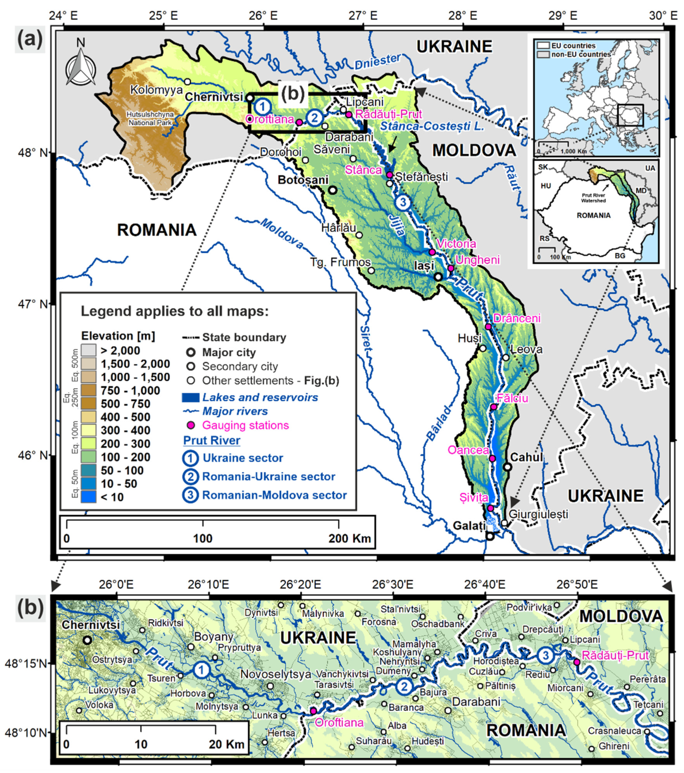
2. Study Area
- Upper watercourse sector: from springs to Cernăuţi where the river flows out of the mountain region. This river sector presents itself as a typical mountain river, with a narrow and deep valley, medium slopes (4.5°) and steep banks. The riverbed has a width of 50–70 m, depth 0.5–1.5 m and rate flow of 1.0–1.5 m/s [13];
- Middle watercourse sector: from Cernăuţi to Ungheni (plain sector) with a floodplain width of 5–6 km with low banks and small slopes (0.1–0.2°). The riverbed has a width of 50–85 m, a depth of 2–3 m and a flow rate of 0.6–1.0 m/s [13];
- Lower watercourse sector: between Ungheni and the confluence with Danube River. The lower course is characterized by small slopes (0.08–0.1°), wide floodplain (10–12 km) and low flow rate (0.5–0.8 m/s). The river has a width of 60–100 m and a depth of 2–4 m [13].
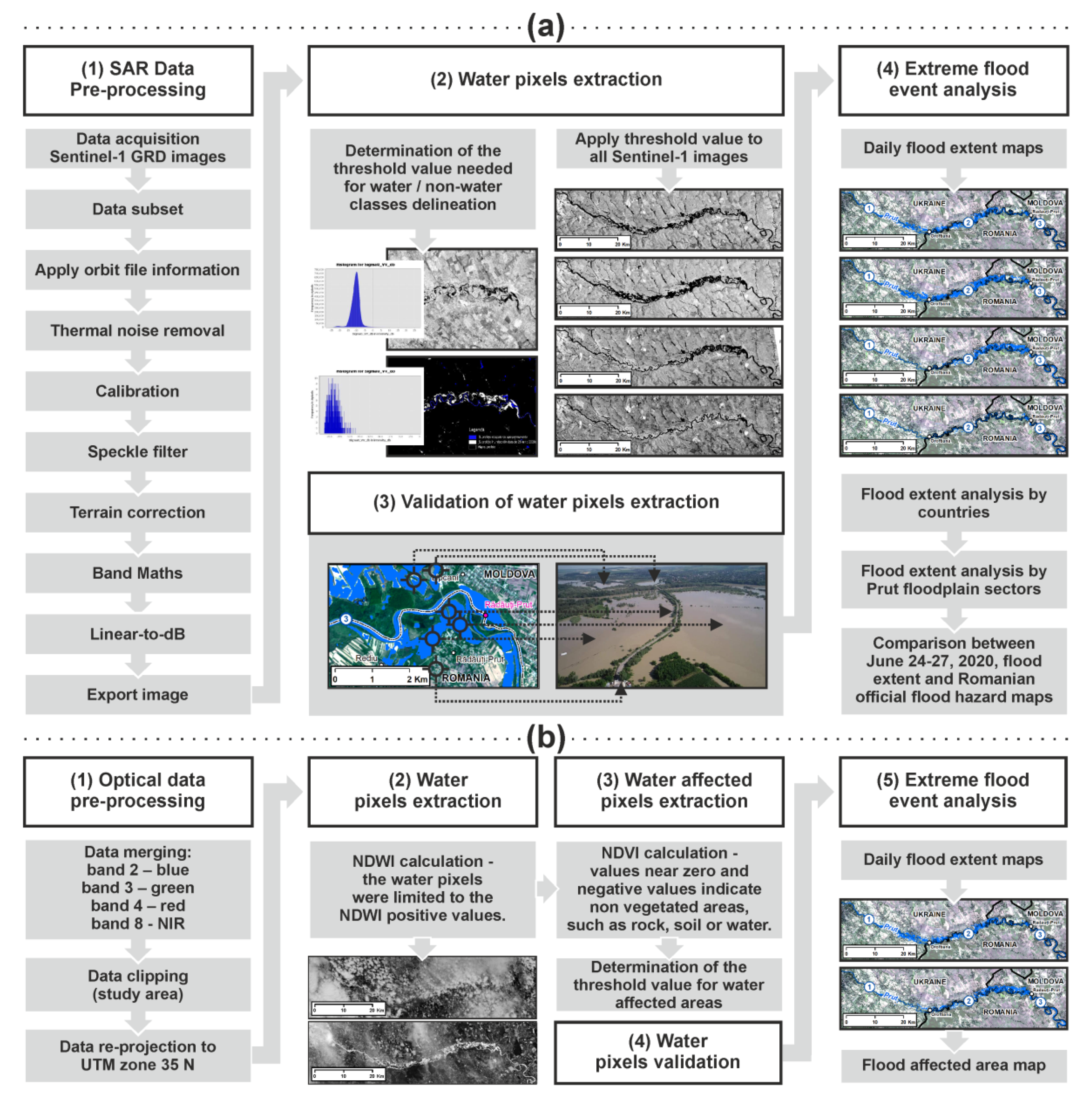
3. Database and Methodology
3.1. Sentinel-1 SAR and Sentinel-2 Data
3.2. SAR and Optical Data Pre-Processing
3.3. Water Pixel Extraction from SAR and Optical Data
3.4. Water-Affected Pixel Extraction from Optical Data
3.5. Water Pixel Validation
3.6. Flood Frequency Analysis
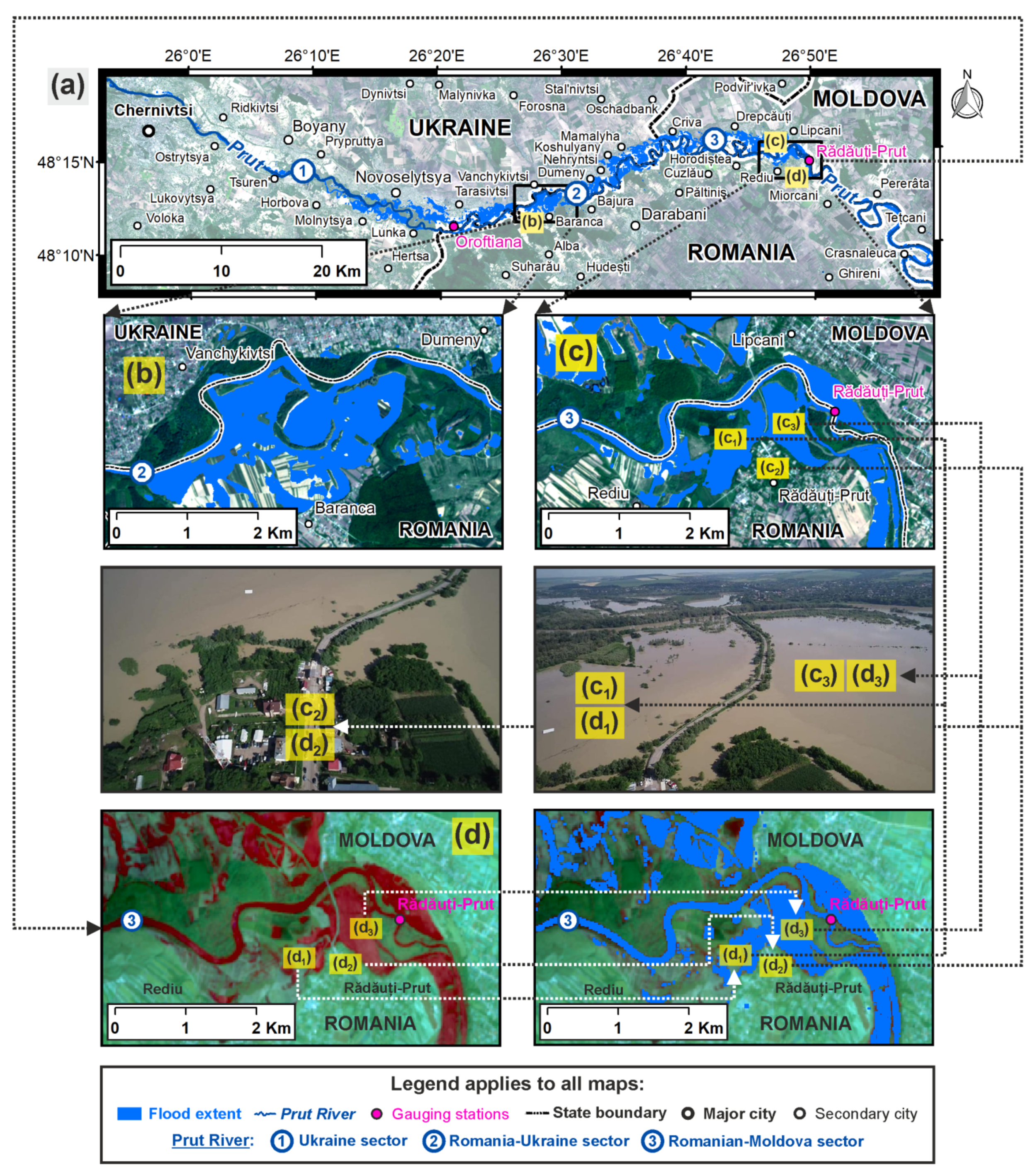
4. Results and Discussion
4.1. Flood Hazard Map
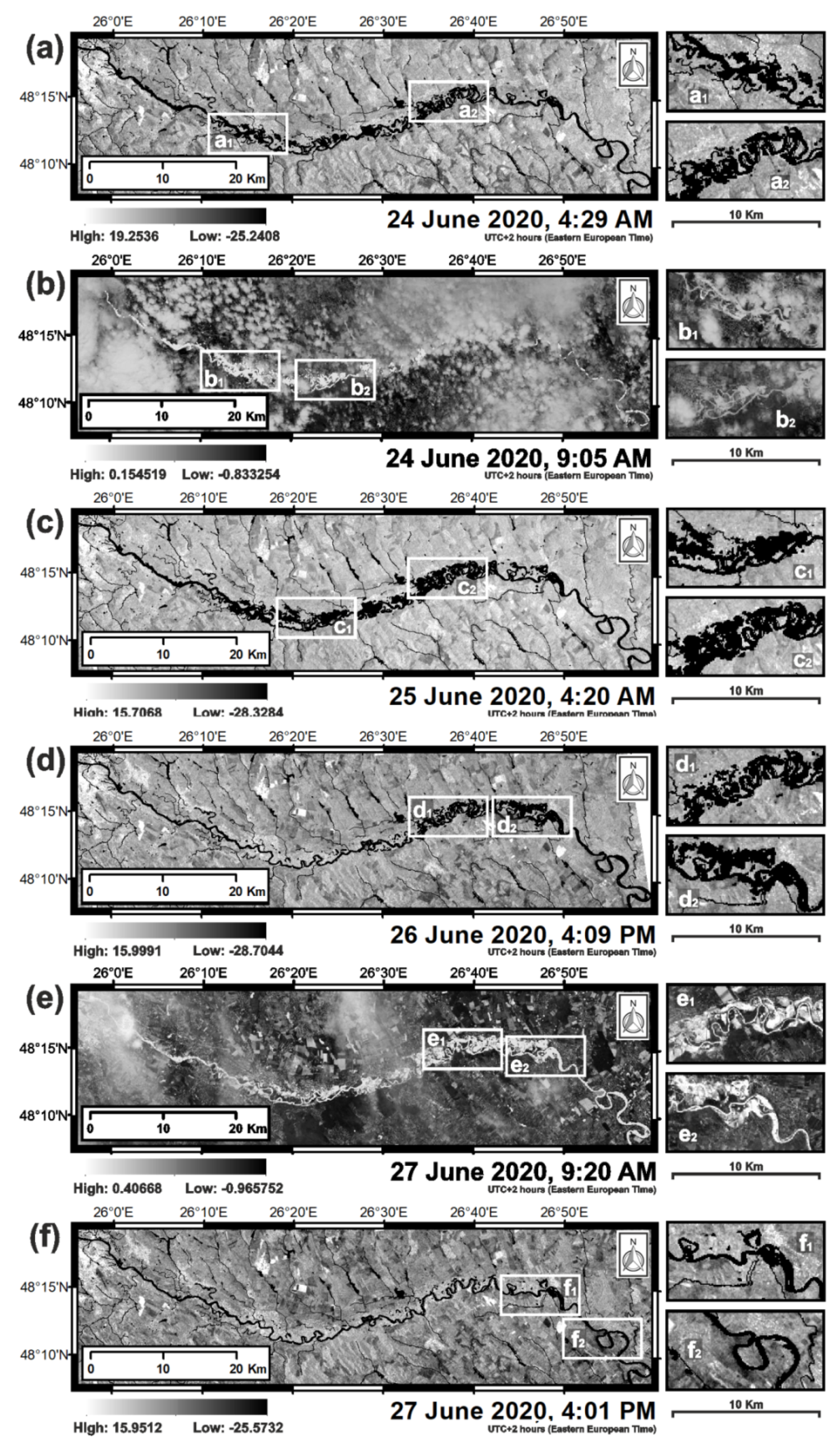
4.2. Flood Wave Development Stages Based of Sentinel-1 SAR Satellite Images
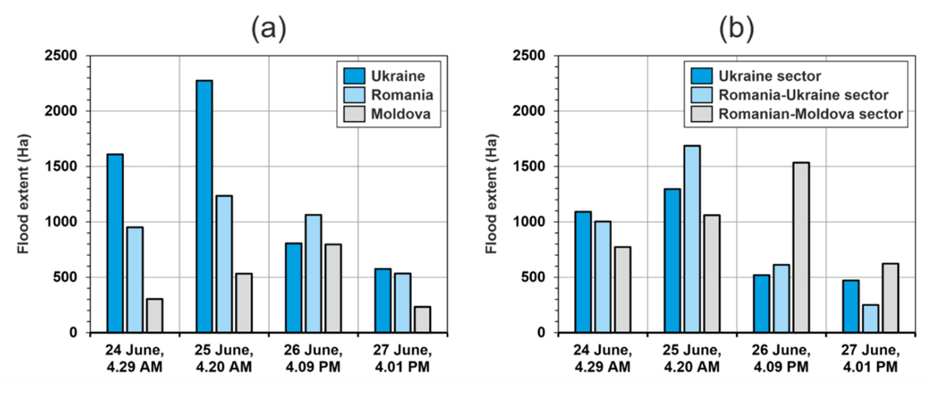
4.2.1. Flood Status on 24 June 2020
4.2.2. Flood Status on 25 June 2020
4.2.3. Flood Status on 26 June 2020
4.2.4. Flood Status on 27 June 2020
4.3. The Sentinel-1 SAR and Sentinel-2 Optical Data: Applicability and Limitations for Flood Assessment
5. Conclusions
Author Contributions
Funding
Institutional Review Board Statement
Informed Consent Statement
Data Availability Statement
Acknowledgments
Conflicts of Interest
Abbreviations
| BoA | Bottom of Atmosphere |
| CM-EMS | Copernicus Mapping—Emergency Management Service |
| DEM | Digital Elevation Model |
| EFD | European Floods Directive |
| EM-DAT | Emergency Events Database |
| ESA | European Space Agency—Copernicus Program |
| EU | European Union |
| EW | Extra-Wide swath |
| FHM | Flood Hazard Maps |
| FRMP | Flood Risk Management Plans |
| FRM | Flood Risk Maps |
| GIS | Geographic Information System |
| GRD | Ground Range Detected |
| HH or VV | Single polarization |
| HH+HV or VV+VH | Dual polarization |
| ICPDR | International Commission for the Protection of the Danube River |
| IW | Interferometric Wide swath |
| LiDAR | Light Intensity Detection and Ranging |
| NDVI | Normalized Difference Vegetation Index |
| NDWI | Normalized Difference Water Index |
| SAR | Synthetic Aperture Radar |
| SLC | Single Look Complex |
| SNAP | Sentinel Application Platform |
| SM | Stripmap |
| SRTM | Shuttle Radar Topography Mission |
| ToA | Top of the Atmosphere |
| UTM 35N | Universal Transverse Mercator—zone 35 North |
| WV | Wave |
References
- Costache, R.; Popa, M.C.; Tien Bui, D.; Diaconu, D.C.; Ciubotaru, N.; Minea, G.; Bao Pham, Q. Spatial predicting of flood potential areas using novel hybridizations of fuzzy decision-making, bivariate statistics, and machine learning. J. Hydrol. 2020, 585, 124808. [Google Scholar] [CrossRef]
- Dumitriu, D. Sediment flux during flood events along the Trotuș River channel: Hydrogeomorphological approach. J. Soils Sediments 2020, 20, 4083–4102. [Google Scholar] [CrossRef]
- Romanescu, G.; Stoleriu, C.C.; Mihu-Pintilie, A. Implementation of EU Water Framework Directive (2000/60/EC) in Romania—European Qualitative Requirements. In Water Resources Management in Romania; Negm, A., Romanescu, G., Zeleňáková, M., Eds.; Springer: Cham, Switzerland, 2020; pp. 17–55. [Google Scholar] [CrossRef]
- Romanescu, G.; Cîmpianu, C.I.; Mihu-Pintilie, A.; Stoleriu, C.C. Historic flood events in NE Romania (post-1990). J. Maps 2017, 13, 787–798. [Google Scholar] [CrossRef]
- Salit, F.; Zaharia, L.; Beltrando, G. Assessment of the warning system against floods on a rural area: The case of the lower Siret River (Romania). Nat. Hazards Earth Syst. Sci. 2013, 13, 409–416. [Google Scholar] [CrossRef] [Green Version]
- Huţanu, E.; Mihu-Pintilie, A.; Urzică, A.; Paveluc, L.E.; Stoleriu, C.C.; Grozavu, A. Using 1D HEC-RAS Modeling and LiDAR Data to Improve Flood Hazard Maps Accuracy: A Case Study from Jijia Floodplain (NE Romania). Water 2020, 12, 1624. [Google Scholar] [CrossRef]
- Romanescu, G.; Mihu-Pintilie, A.; Stoleriu, C.C.; Carboni, D.; Paveluc, L.; Cîmpianu, C.I. A Comparative Analysis of Exceptional Flood Events in the Context of Heavy Rains in the Summer of 2010: Siret Basin (NE Romania) Case Study. Water 2018, 10, 216. [Google Scholar] [CrossRef] [Green Version]
- Mihu-Pintilie, A.; Cîmpianu, C.I.; Stoleriu, C.C.; Pérez, M.N.; Paveluc, L.E. Using High-Density LiDAR Data and 2D Streamflow Hydraulic Modeling to Improve Urban Flood Hazard Maps: A HEC-RAS Multi-Scenario Approach. Water 2019, 11, 1832. [Google Scholar] [CrossRef] [Green Version]
- Mihu-Pintilie, A.; Nicu, I.C. GIS-based Landform Classification of Eneolithic Archaeological Sites in the Plateau-plain Transition Zone (NE Romania): Habitation Practices vs. Flood Hazard Perception. Remote Sens. 2019, 11, 915. [Google Scholar] [CrossRef] [Green Version]
- EM-DAT (Emergency Events Database). The Emergency Events Database of Université Catholique de Louvain (UCL)—CRED, D. Guha-Sapir, Brussels, Belgium. Available online: https://www.emdat.be (accessed on 25 October 2021).
- Stoleriu, C.C.; Urzică, A.; Mihu-Pintilie, A. Improving flood risk map accuracy using high-density LiDAR data and the HEC-RAS river analysis system: A case study from north-eastern Romania. J. Flood Risk Manag. 2020, 13, e12572. [Google Scholar] [CrossRef]
- Romanescu, G.; Stoleriu, C.C.; Romanescu, A.-M. Water reservoirs and the risk of accidental flood occurrence. Case study: Stanca–Costesti reservoir and the historical floods of the Prut river in the period July–August 2008, Romania. Hydrol. Process. 2011, 25, 2056–2070. [Google Scholar] [CrossRef]
- Stoleriu, C.C.; Romanescu, G.; Mihu-Pintilie, A. Using single-beam echo-sounder for assessing the silting rate from the largest cross-border reservoir of the Eastern Europe: Stanca-Costesti Lake, Romania and Republic of Moldova. Carpathian J. Earth Environ. Sci. 2019, 14, 83–94. [Google Scholar] [CrossRef]
- Costache, R. Flood Susceptibility Assessment by Using Bivariate Statistics and Machine Learning Models—A Useful Tool for Flood Risk Management. Water Resour. Manag. 2019, 33, 3239–3256. [Google Scholar] [CrossRef]
- Irimescu, A.; Stancalie, G.; Craciunescu, V.; Flueraru, C.; Anderson, E. The Use of Remote Sensing and GIS Techniques in Flood Monitoring and Damage Assessment: A Study Case in Romania. In Threats to Global Water Security. NATO Science for Peace and Security, Series C: Environmental Security; Jones, J.A.A., Vardanian, T.G., Hakopian, C., Eds.; Springer: Cham, Switzerland, 2009; pp. 167–177. [Google Scholar] [CrossRef]
- Arseni, M.; Rosu, A.; Calmuc, M.; Calmuc, V.A.; Iticescu, C.; Georgescu, L.P. Development of Flood Risk and Hazard Maps for the Lower Course of the Siret River, Romania. Sustainability 2020, 12, 6588. [Google Scholar] [CrossRef]
- Romanescu, G.; Stoleriu, C.C. An inter-basin backwater overflow (the Buhai Brook and the Ezer reservoir on the Jijia River, Romania). Hydrol. Process. 2013, 28, 3118–3131. [Google Scholar] [CrossRef]
- Romanescu, G.; Stoleriu, C.C. Exceptional floods in the Prut basin, Romania, in the context of heavy rains in the summer of 2010. Nat. Hazards Earth Syst. Sci. 2017, 17, 381–396. [Google Scholar] [CrossRef] [Green Version]
- ICPDR (International Commission for the Protection of the Danube River). Flood Action Programme Prut-Siret Sub-Basin. Available online: http://www.icpdr.org/main/activities-projects/flood-action-plans (accessed on 25 October 2021).
- Kjeldsen, T.R.; Macdonald, N.; Lang, M.; Mediero, L.; Albuquerque, T.; Bogdanowicz, E.; Brázdil, R.; Castellarin, A.; David, V.; Fleig, A.; et al. Documentary evidence of past floods in Europe and their utility in flood frequency estimation. J. Hydrol. 2014, 517, 963–973. [Google Scholar] [CrossRef] [Green Version]
- Ezzine, A.; Saidi, S.; Hermassi, T.; Kammessi, I.; Darragi, F.; Rajhi, H. Flood mapping using hydraulic modeling and Sentinel-1 image: Case study of Medjerda Basin, northern Tunisia. Egypt. J. Remote Sens. Space Sci. 2020, 23, 303–310. [Google Scholar] [CrossRef]
- Horritt, M.S.; Bates, P.D. Evaluation of 1D and 2D numerical models for predicting river flood inundation. J. Hydrol. 2002, 268, 87–99. [Google Scholar] [CrossRef]
- Machado, M.J.; Botero, B.A.; López, J.; Francés, F.; Díez-Herrero, A.; Benito, G. Flood frequency analysis of historical flood data under stationary and non-stationary modelling. Hydrol. Earth Syst. Sci. 2015, 19, 2561–2576. [Google Scholar] [CrossRef] [Green Version]
- Samela, C.; Albano, R.; Sole, A.; Manfreda, S. A GIS tool for cost-effective delineation of flood-prone areas. Comput. Environ. Urban Syst. 2018, 70, 43–52. [Google Scholar] [CrossRef]
- Guerriero, L.; Ruzza, G.; Guadagno, F.M.; Revellino, P. Flood hazard mapping incorporating multiple probability models. J. Hydrol. 2020, 587, 125020. [Google Scholar] [CrossRef]
- Islam, M.M.; Sado, K. Development of flood hazard maps of Bangladesh using NOAA-AVHRR images with GIS. Hydrol. Sci. J. 2000, 45, 337–355. [Google Scholar] [CrossRef]
- Schumann, G.J.-P.; Domeneghetti, A. Exploiting the proliferation of current and future satellite observations of rivers. Hydrol. Process. 2016, 30, 2891–2896. [Google Scholar] [CrossRef]
- Huang, C.; Chen, Y.; Wu, J. Mapping spatio-temporal flood inundation dynamics at large river basin scale using time-series flow data and MODIS imagery. Int. J. Appl. Earth Obs. Geoinf. 2014, 26, 350–362. [Google Scholar] [CrossRef]
- Rahman, M.S.; Di, L. The state of the art of spaceborne remote sensing in flood management. Nat. Hazards 2017, 85, 1223–1248. [Google Scholar] [CrossRef]
- Sanyal, J.; Lu, X.X. Application of remote sensing in flood management with special reference to monsoon Asia: A review. Nat. Hazards 2004, 33, 283–301. [Google Scholar] [CrossRef]
- Borah, S.B.; Sivasankar, T.; Ramya, M.N.S.; Raju, P.L.N. Flood inundation mapping and monitoring in Kaziranga National Park, Assam using Sentinel-1 SAR data. Environ. Monit. Assess. 2018, 190, 520. [Google Scholar] [CrossRef] [PubMed]
- Chowdhury, E.H.; Hassan, Q.K. Use of remote sensing data in comprehending an extremely unusual flooding event over southwest Bangladesh. Nat. Hazards 2017, 88, 1805–1823. [Google Scholar] [CrossRef]
- Hoque, R.; Nakayama, D.; Matsuyama, H.; Matsumoto, J. Flood monitoring, mapping and assessing capabilities using RADARSAT remote sensing, GIS and ground data for Bangladesh. Nat. Hazards 2011, 57, 525–548. [Google Scholar] [CrossRef]
- Schumann, G.; Moller, D.K. Microwave remote sensing of flood inundation. Phys. Chem. Earth 2015, 83–84, 84–95. [Google Scholar] [CrossRef]
- Twele, A.; Cao, W.; Plank, S.; Martinis, S. Sentinel-1- based flood mapping: A fully automated processing chain. Int. J. Remote Sens. 2016, 37, 2990–3004. [Google Scholar] [CrossRef]
- Amitrano, D.; Martino, G.D.; Iodice, A.; Mitidieri, F.; Papa, M.N.; Riccio, D.; Ruello, G. Sentinel-1 for Monitoring Reservoirs: A Performance Analysis. Remote Sens. 2014, 6, 10676–10693. [Google Scholar] [CrossRef] [Green Version]
- Landuyt, L.; Verhoest, N.E.K.; van Coillie, F.M.B. Flood Mapping in Vegetated Areas Using an Unsupervised Clustering Approach on Sentinel-1 and -2 Imagery. Remote Sens. 2020, 12, 3611. [Google Scholar] [CrossRef]
- Malenovský, Z.; Helmut, R.; Cihlar, J.; Schaepman, M.E.; García-Santos, G.; Fernandes, R.; Berger, M. Sentinels for science: Potential of Sentinel-1, -2, and -3 missions for scientific observations of ocean, cryosphere, and land. Remote Sens. Environ. 2012, 120, 91–101. [Google Scholar] [CrossRef]
- Poursanidis, D.; Chrysoulakis, N. Remote Sensing, natural hazards and the contribution of ESA Sentinels missions. Remote Sens. Appl. Soc. Environ. 2017, 6, 25–38. [Google Scholar] [CrossRef]
- Gebremichael, E.; Molthan, A.L.; Bell, J.R.; Schultz, L.A.; Hain, C. Flood Hazard and Risk Assessment of Extreme Weather Events Using Synthetic Aperture Radar and Auxiliary Data: A Case Study. Remote Sens. 2020, 12, 3588. [Google Scholar] [CrossRef]
- Huang, M.; Jin, S. Rapid Flood Mapping and Evaluation with a Supervised Classifier and Change Detection in Shouguang Using Sentinel-1 SAR and Sentinel-2 Optical Data. Remote Sens. 2020, 12, 2073. [Google Scholar] [CrossRef]
- Li, Y.; Martinis, S.; Plank, S.; Ludwig, R. An automatic change detection approach for rapid flood mapping in Sentinel-1 SAR data. Int. J. Appl. Earth Obs. Geoinf. 2018, 73, 123–135. [Google Scholar] [CrossRef]
- Romero, N.A.; Cigna, F.; Tapete, D. ERS-1/2 and Sentinel-1 SAR Data Mining for Flood Hazard and Risk Assessment in Lima, Peru. Appl. Sci. 2020, 10, 6598. [Google Scholar] [CrossRef]
- Tapete, D.; Cigna, F. Poorly known 2018 floods in Bosra UNESCO site and Sergiopolis in Syria unveiled from space using Sentinel-1/2 and COSMO-SkyMed. Sci. Rep. 2020, 10, 12307. [Google Scholar] [CrossRef] [PubMed]
- Konapala, G.; Kumar, S.V.; Ahmad, S.K. Exploring Sentinel-1 and Sentinel-2 diversity for flood inundation mapping using deep learning. Isprs J. Photogramm. Remote Sens. 2021, 180, 163–173. [Google Scholar] [CrossRef]
- Burcea, S.; Cică, R.; Bojariu, R. Radar-derived convective storms’ climatology for the Prut River basin: 2003–2017. Nat. Hazards Earth Syst. Sci. 2019, 19, 1305–1318. [Google Scholar] [CrossRef] [Green Version]
- Bamler, R. Principles of Synthetic Aperture Radar. Surv. Geophys. 2000, 21, 147–157. [Google Scholar] [CrossRef]
- Moreira, A.; Prats-Iraola, P.; Younis, M.; Krieger, G.; Hajnsek, I.; Papathanassiou, K.P. A Tutorial on Synthetic Aperture Radar. IEEE Geosci. Remote Sens. Mag. 2013, 1, 6–43. [Google Scholar] [CrossRef] [Green Version]
- Aschbacher, J.; Milagro-Pérez, M.P. The European Earth monitoring (GMES) programme: Status and perspectives. Remote Sens. Environ. 2012, 120, 3–8. [Google Scholar] [CrossRef]
- Clement, M.; Kilsby, C.; Moore, P. Multi-temporal synthetic aperture radar flood mapping using change detection. J. Flood Risk Manag. 2018, 11, 152–168. [Google Scholar] [CrossRef]
- Tsyganskaya, V.; Martinis, S.; Marzahn, P.; Ludwig, R. Detection of Temporary Flooded Vegetation Using Sentinel-1 Time Series Data. Remote Sens. 2018, 10, 1286. [Google Scholar] [CrossRef] [Green Version]
- DeVries, B.; Huang, C.; Armston, J.; Huang, W.; Jones, J.W.; Lange, M.W. Rapid and robust monitoring of flood events using Sentinel-1 and Landsat data on the Google Earth Engine. Remote Sens. Environ. 2020, 240, 111664. [Google Scholar] [CrossRef]
- Chojka, A.; Artiemjew, P.; Rapiński, J. RFI Artefacts Detection in Sentinel-1 Level-1 SLC Data Based On Image Processing Techniques. Sensors 2020, 20, 2919. [Google Scholar] [CrossRef]
- Stasolla, M.; Neyt, X. An Operational Tool for the Automatic Detection and Removal of Border Noise in Sentinel-1 GRD Products. Sensors 2018, 18, 3454. [Google Scholar] [CrossRef] [Green Version]
- Muro, J.; Canty, M.; Conradsen, K.; Hüttich, C.; Nielsen, A.A.; Skriver, H.; Remy, F.; Strauch, A.; Thonfeld, F.; Menz, G. Short-Term Change Detection in Wetlands Using Sentinel-1 Time Series. Remote Sens. 2016, 8, 795. [Google Scholar] [CrossRef] [Green Version]
- Goumehei, E.; Tolpekin, V.; Stein, A.; Yan, W. Surface water body detection in polarimetric SAR data using contextual complex Wishart classification. Water Resour. Res. 2019, 55, 7047–7059. [Google Scholar] [CrossRef] [Green Version]
- Schubert, A.; Miranda, N.; Geudtner, D.; Small, D. Sentinel-1A/B Combined Product Geolocation Accuracy. Remote Sens. 2017, 9, 607. [Google Scholar] [CrossRef] [Green Version]
- Clauss, K.; Ottinger, M.; Leinenkugel, P.; Kuenzer, C. Estimating rice production in the Mekong Delta, Vietnam, utilizing time series of Sentinel-1 SAR data. Int. J. Appl. Earth Obs. Geoinf. 2018, 73, 574–585. [Google Scholar] [CrossRef]
- Carreño Conde, F.; de Mata Muñoz, M. Flood Monitoring Based on the Study of Sentinel-1 SAR Images: The Ebro River Case Study. Water 2019, 11, 2454. [Google Scholar] [CrossRef] [Green Version]
- Li, X.; Zhou, Y.; Gong, P.; Seto, K.C.; Clinton, N. Developing a method to estimate building height from Sentinel-1 data. Remote Sens. Environ. 2020, 240, 111705. [Google Scholar] [CrossRef]
- Perrou, T.; Garioud, A.; Parcharidis, I. Use of Sentinel-1 imagery for flood management in a reservoir-regulated river basin. Front. Earth Sci. 2018, 12, 506–520. [Google Scholar] [CrossRef]
- Huth, J.; Gessner, U.; Klein, I.; Yesou, H.; Lai, X.; Oppelt, N.; Kuenzer, C. Analyzing Water Dynamics Based on Sentinel-1 Time Series—A Study for Dongting Lake Wetlands in China. Remote Sens. 2020, 12, 1761. [Google Scholar] [CrossRef]
- Goffi, A.; Stroppiana, D.; Brivio, P.A.; Bordogna, G.; Boschetti, M. Towards an automated approach to map flooded areas from Sentinel-2 MSI data and soft integration of water spectral features. Int. J. Appl. Earth Obs. Geoinf. 2020, 84, 101951. [Google Scholar] [CrossRef]
- Cordeiro, M.C.R.; Martinez, J.-M.; Peña-Luque, S. Automatic water detection from multidimensional hierarchical clustering for Sentinel-2 images and a comparison with Level 2A processors. Remote Sens. Environ. 2021, 253, 112209. [Google Scholar] [CrossRef]
- Pahlevan, N.; Sarkar, S.; Franz, B.A.; Balasubramanian, S.V.; He, J. Sentinel-2 MultiSpectral Instrument (MSI) data processing for aquatic science applications: Demonstrations and validations. Remote Sens. Environ. 2017, 201, 47–56. [Google Scholar] [CrossRef]
- Szantoi, Z.; Strobl, P. Copernicus Sentinel-2 Calibration and Validation. Eur. J. Remote Sens. 2019, 52, 253–255. [Google Scholar] [CrossRef] [Green Version]
- Huang, W.; DeVries, B.; Huang, C.; Lang, M.W.; Jones, J.W.; Creed, I.F.; Carroll, M.L. Automated Extraction of Surface Water Extent from Sentinel-1 Data. Remote Sens. 2018, 10, 797. [Google Scholar] [CrossRef] [Green Version]
- Manakos, I.; Kordelas, G.A.; Marini, K. Fusion of Sentinel-1 data with Sentinel-2 products to overcome non-favourable atmospheric conditions for the delineation of inundation maps. Eur. J. Remote Sens. 2020, 53, 53–66. [Google Scholar] [CrossRef] [Green Version]
- Pulvirenti, L.; Chini, M.; Pierdicca, N.; Boni, G. Use of SAR Data for Detecting Floodwater in Urban and Agricultural Areas: The Role of the Interferometric Coherence. IEEE Trans. Geosci. Remote Sens. 2016, 54, 1532–1544. [Google Scholar] [CrossRef]
- Singha, M.; Dong, J.; Sarmah, S.; You, N.; Zhou, Y.; Zhang, G.; Doughty, R.; Xiao, X. Identifying floods and flood-affected paddy rice fields in Bangladesh based on Sentinel-1 imagery and Google Earth Engine. Isprs J. Photogramm. Remote Sens. 2020, 166, 278–293. [Google Scholar] [CrossRef]
- Leroux, L.; Congedo, L.; Bellón, B.; Gaetano, R.; Bégué, A. Land Cover Mapping Using Sentinel-2 Images and the Semi-Automatic Classification Plugin: A Northern Burkina Faso Case Study. In QGIS and Applications in Agriculture and Forest; Baghdadi, N., Mallet, C., Zribi, M., Eds.; Wiley: Hoboken, NJ, USA, 2018; pp. 119–151. [Google Scholar] [CrossRef]
- Clerici, N.; Valbuena Calderón, C.A.; Posada, J.M. Fusion of Sentinel-1A and Sentinel-2A data for land cover mapping: A case study in the lower Magdalena region, Colombia. J. Maps 2017, 13, 718–726. [Google Scholar] [CrossRef] [Green Version]
- Truckenbrodt, J.; Freemantle, T.; Williams, C.; Jones, T.; Small, D.; Dubois, C.; Thiel, C.; Rossi, C.; Syriou, A.; Giuliani, G. Towards Sentinel-1 SAR Analysis-Ready Data: A Best Practices Assessment on Preparing Backscatter Data for the Cube. Data 2019, 4, 93. [Google Scholar] [CrossRef] [Green Version]
- Filipponi, F. Sentinel-1 GRD Preprocessing Workflow. In Proceedings of the 3rd International Electronic Conference on Remote Sensing (ECRS 2019), Online, 22 May–5 June 2019. [Google Scholar] [CrossRef] [Green Version]
- Mandal, D.; Kumar, V.; Rathaa, D.; Dey, S.; Bhattacharyaa, A.; Lopez-Sanchez, J.M.; McNairn, H.; Rao, Y.S. Dual polarimetric radar vegetation index for crop growth monitoring using sentinel-1 SAR data. Remote Sens. Environ. 2020, 247, 111954. [Google Scholar] [CrossRef]
- Hu, S.; Qin, J.; Ren, J.; Zhao, H.; Ren, J.; Hong, H. Automatic Extraction of Water Inundation Areas Using Sentinel-1 Data for Large Plain Areas. Remote Sens. 2020, 12, 243. [Google Scholar] [CrossRef] [Green Version]
- Gašparović, M.; Dobrinić, D. Comparative Assessment of Machine Learning Methods for Urban Vegetation Mapping Using Multitemporal Sentinel-1 Imagery. Remote Sens. 2020, 12, 1952. [Google Scholar] [CrossRef]
- Mirsoleimani, H.R.; Sahebi, M.R.; Baghdadi, N.; El Hajj, M. Bare Soil Surface Moisture Retrieval from Sentinel-1 SAR Data Based on the Calibrated IEM and Dubois Models Using Neural Networks. Sensors 2019, 19, 3209. [Google Scholar] [CrossRef] [Green Version]
- Benoudjit, A.; Guida, R. A Novel Fully Automated Mapping of the Flood Extent on SAR Images Using a Supervised Classifier. Remote Sens. 2019, 11, 779. [Google Scholar] [CrossRef] [Green Version]
- Prasad, K.A.; Ottinger, M.; Wei, C.; Leinenkugel, P. Assessment of Coastal Aquaculture for India from Sentinel-1 SAR Time Series. Remote Sens. 2019, 11, 357. [Google Scholar] [CrossRef] [Green Version]
- Ahmad, W.; Kim, D. Estimation of flow in various sizes of streams using the Sentinel-1 Synthetic Aperture Radar (SAR) data in Han River Basin, Korea. Int. J. Appl. Earth Obs. Geoinf. 2019, 83, 101930. [Google Scholar] [CrossRef]
- Liu, Y.; Gong, W.; Xing, Y.; Hu, X.; Gong, J. Estimation of the forest stand mean height and above ground biomass in Northeast China using SAR Sentinel-1B, multispectral Sentinel-2A, and DEM imagery. Isprs J. Photogramm. Remote Sens. 2019, 151, 277–289. [Google Scholar] [CrossRef]
- Ye, Y.; Yang, C.; Zhu, B.; Zhou, L.; He, Y.; Jia, H. Improving Co-Registration for Sentinel-1 SAR and Sentinel-2 Optical Images. Remote Sens. 2021, 13, 928. [Google Scholar] [CrossRef]
- Matgen, P.; Hostache, R.; Schumann, G.; Pfister, L.; Hoffmann, L.; Savenije, H.H.G. Towards an automated SAR-based flood monitoring system: Lessons learned from two case studies. Phys. Chem. Earth 2011, 36, 241–252. [Google Scholar] [CrossRef]
- Chini, M.; Pelich, R.; Pulvirenti, L.; Pierdicca, N.; Hostache, R.; Matgen, P. Sentinel-1 InSAR Coherence to Detect Floodwater in Urban Areas: Houston and Hurricane Harvey as A Test Case. Remote Sens. 2019, 11, 107. [Google Scholar] [CrossRef] [Green Version]
- Wan, L.; Liu, M.; Wang, F.; Zhang, T.; You, H.J. Automatic extraction of flood inundation areas from SAR images: A case study of Jilin, China during the 2017 flood disaster. Int. J. Remote Sens. 2019, 40, 5050–5077. [Google Scholar] [CrossRef]
- Gstaiger, V.; Huth, J.; Gebhardt, S.; Wehrmann, T.; Kuenzer, C. Multi-sensoral and automated derivation of inundated areas using TerraSAR-X and ENVISAT ASAR data. Int. J. Remote Sens. 2012, 33, 7291–7304. [Google Scholar] [CrossRef]
- Liang, J.; Liu, D. A local thresholding approach to flood water delineation using Sentinel-1 SAR imagery. Isprs J. Photogramm. Remote Sens. 2020, 159, 53–62. [Google Scholar] [CrossRef]
- Lu, J.; Giustarini, L.; Xiong, B.; Zhao, L.; Jiang, Y.; Kuang, G. Automated flood detection with improved robustness and efficiency using multitemporal SAR data. Remote Sens. Lett. 2014, 5, 240–248. [Google Scholar] [CrossRef]
- Gan, T.Y.; Zunic, F.; Kuo, C.-C.; Strobl, T. Flood mapping of Danube River at Romania using single and multi-date ERS2-SAR images. Int. J. Appl. Earth Obs. Geoinf. 2012, 18, 69–81. [Google Scholar] [CrossRef]
- Rahman, M.R.; Thakur, P.K. Detecting, mapping and analysing of flood water propagation using synthetic aperture radar (SAR) satellite data and GIS: A case study from the Kendrapara District of Orissa State of India. Egypt. J. Remote Sens. Space Sci. 2018, 21, S37–S41. [Google Scholar] [CrossRef]
- McFeeters, S.K. The use of the Normalized Difference Water Index (NDWI) in the delineation of open water features. Int. J. Remote Sens. 1996, 17, 1425–1432. [Google Scholar] [CrossRef]
- Du, Y.; Zhang, Y.; Ling, F.; Wang, Q.; Li, W.; Li, X. Water Bodies’ Mapping from Sentinel-2 Imagery with Modified Normalized Difference Water Index at 10-m Spatial Resolution Produced by Sharpening the SWIR Band. Remote Sens. 2016, 8, 354. [Google Scholar] [CrossRef] [Green Version]
- Yang, X.; Zhao, S.; Qin, X.; Zhao, N.; Liang, L. Mapping of Urban Surface Water Bodies from Sentinel-2 MSI Imagery at 10 m Resolution via NDWI-Based Image Sharpening. Remote Sens. 2017, 9, 596. [Google Scholar] [CrossRef] [Green Version]
- Jiang, W.; Ni, Y.; Pang, Z.; Li, X.; Ju, H.; He, G.; Lv, J.; Yang, K.; Fu, J.; Qin, X. An Effective Water Body Extraction Method with New Water Index for Sentinel-2 Imagery. Water 2021, 13, 1647. [Google Scholar] [CrossRef]
- Bangira, T.; Alfieri, S.M.; Menenti, M.; van Niekerk, A.; Vekerdy, Z. A Spectral Unmixing Method with Ensemble Estimation of Endmembers: Application to Flood Mapping in the Caprivi Floodplain. Remote Sens. 2017, 9, 1013. [Google Scholar] [CrossRef] [Green Version]
- Gargiulo, M.; Dell’Aglio, D.A.G.; Iodice, A.; Riccio, D.; Ruello, G. Integration of Sentinel-1 and Sentinel-2 Data for Land Cover Mapping Using W-Net. Sensors 2020, 20, 2969. [Google Scholar] [CrossRef] [PubMed]
- Notti, D.; Giordan, D.; Caló, F.; Pepe, A.; Zucca, F.; Galve, J.P. Potential and Limitations of Open Satellite Data for Flood Mapping. Remote Sens. 2018, 10, 1673. [Google Scholar] [CrossRef] [Green Version]
- Saravanan, S.; Jegankumar, R.; Selvaraj, A.; Jacinth Jennifer, J.; Parthasarathy, K.S.S. Chapter 20—Utility of landsat data for assessing mangrove degradation in Muthupet Lagoon, South India. Coast. Zone Manag. 2019, 20, 471–484. [Google Scholar] [CrossRef]
- CM-EMS (Copernicus Mapping—Emergency Management Service). EMSR445: Flood in Romania. Available online: https://emergency.copernicus.eu/mapping/list-of-components/EMSR445 (accessed on 25 October 2021).
- Gumbel, E.J. The return period of flood flows. Ann. Math. Stat. 1941, 12, 163–190. [Google Scholar] [CrossRef]
- Bhat, M.; Alam, A.; Ahmad, B.; Kotlia, B.S.; Farooq, H.; Taloor, A.K.; Ahmad, S. Flood frequency analysis of river Jhelum in Kashmir basin. Quat. Int. 2019, 507, 288–294. [Google Scholar] [CrossRef]
- Farooq, M.; Shafique, M.; Khattak, M.S. Flood frequency analysis of river swat using Log Pearson type 3, Generalized Extreme Value, Normal, and Gumbel Max distribution methods. Arab. J. Geosci. 2018, 11, 216. [Google Scholar] [CrossRef]
- Kumar, R. Flood Frequency Analysis of the Rapti River Basin using Log Pearson Type-III and Gumbel Extreme Value-1 Methods. J. Geol. Soc. India 2019, 94, 480–484. [Google Scholar] [CrossRef]


| Gauge Station | Year of Inauguration | Elevation (m a.s.l.) | Latitude | Longitude | Max. Water Level Recorded (cm) | Max. Flow Rate Recorded (m3/s) | Date of Max. Flow Rate |
|---|---|---|---|---|---|---|---|
| Oroftiana 1 | 1976 | 123.47 | 48°11′12″ | 26°21′04″ | 876 | - | - |
| Rădăuți-Prut | 1976 | 101.87 | 48°14′55″ | 26°48′14″ | 1130 | 4240 | 28 July 2008 |
| Stânca Aval | 1978 | 62.00 | 47°47′00″ | 27°16′00″ | 512 | 1050 | 31 July 2008 |
| Ungheni | 1914 | 31.41 | 47°11′04″ | 27°48′28″ | 654 | 796 | 8–10 July 2010 |
| Prisăcani | 1976 | 28.08 | 47°05′19″ | 27°53′38″ | 622 | 900 | 9–10 July 2010 |
| Drânceni | 1915 | 18.65 | 46°48′45″ | 28°08′04″ | 718 | 736 | 17–18 July 2010 |
| Fălciu | 1927 | 10.04 | 46°18′52″ | 28°09′13″ | 650 | 722 | 19 July 2010 |
| Oancea | 1928 | 6.30 | 45°53′37″ | 28°03′04″ | 622 | 757 | 24 April 1979 |
| Șivița 2 | 1978 | 1.66 | 45°37′10″ | 28°05′23″ | - | - | - |
| ID | Image Identifier | Satellite | Date Acquired/Time | Product Type | Mode | Polarization |
|---|---|---|---|---|---|---|
| A | S1A_IW_GRDH_1SDV_20200624T042904_20200624T042929_033154_03D73C_540B | S1A | 2020-06-24/T04:29:04.880Z | GRD | IW | VV VH |
| B | S2B_MSIL2A_20200624T090559_N0214_R050_T35UMP_20200624T123246 | S2B | 2020-06-24/T09:05:59.024Z | LEVEL-2A | - | - |
| C | S1B_IW_GRDH_1SDV_20200625T042007_20200625T042036_022185_02A1B4_C73E | S1B | 2020-06-25/T04:20:07.597Z | GRD | IW | VV VH |
| D | S1B_IW_GRDH_1SDV_20200626T160915_20200626T160940_022207_02A256_2724 | S1B | 2020-06-26/T16:09:15.797Z | GRD | IW | VV VH |
| E | S2B_MSIL2A_20200627T092029_N0214_R093_T35UMP_20200627T121756 | S2B | 2020-06-27/T09:20:29.024Z | LEVEL-2A | - | - |
| F | S1A_IW_GRDH_1SDV_20200627T160148_20200627T160213_033205_03D8C4_F195 | S1A | 2020-06-27/T16:01:48.625Z | GRD | IW | VV VH |
| Return Period (T) in Years | Probability of Occurrence (%) | Reduced Variate (Yt) | Frequency Factor (K) | Computed Flood Discharges (XT) (m³/s) |
|---|---|---|---|---|
| 1000 | 0.1 | 6.907255 | 5.5528495 | 5191.5417 |
| 100 | 1 | 4.600149 | 3.539316 | 3670.2634 |
| 33.3 | 3 | 3.491366 | 2.571624 | 2939.1456 |
| 20 | 5 | 2.970195 | 2.116770 | 2595.4911 |
| 10 | 10 | 2.250367 | 1.488538 | 2120.8451 |
| 5 | 20 | 1.499939 | 0.833600 | 1626.0222 |
| Date | Flow Rate (m3/s)/Time of Image Acquisition | Probability of Occurrence (%)/Time of Image Acquisition | Maximum Flow Rate (m3/s) of the Day | Maximum Probability of Occurrence (%) of the Day |
|---|---|---|---|---|
| 24 June 2020 | 990/4:29 AM | 32.84/4:29 AM | 1585 | 20.51 |
| 25 June 2020 | 1705/4:20 AM | 19.07/4:20 AM | 2610 | 4.97 |
| 26 June 2020 | 2860/4:09 PM | 3.08/4:09 PM | 2965 | 2.97 |
| 27 June 2020 | 2410/4:01 PM | 5.38/4:01 PM | - | - |
Publisher’s Note: MDPI stays neutral with regard to jurisdictional claims in published maps and institutional affiliations. |
© 2021 by the authors. Licensee MDPI, Basel, Switzerland. This article is an open access article distributed under the terms and conditions of the Creative Commons Attribution (CC BY) license (https://creativecommons.org/licenses/by/4.0/).
Share and Cite
Cîmpianu, C.I.; Mihu-Pintilie, A.; Stoleriu, C.C.; Urzică, A.; Huţanu, E. Managing Flood Hazard in a Complex Cross-Border Region Using Sentinel-1 SAR and Sentinel-2 Optical Data: A Case Study from Prut River Basin (NE Romania). Remote Sens. 2021, 13, 4934. https://0-doi-org.brum.beds.ac.uk/10.3390/rs13234934
Cîmpianu CI, Mihu-Pintilie A, Stoleriu CC, Urzică A, Huţanu E. Managing Flood Hazard in a Complex Cross-Border Region Using Sentinel-1 SAR and Sentinel-2 Optical Data: A Case Study from Prut River Basin (NE Romania). Remote Sensing. 2021; 13(23):4934. https://0-doi-org.brum.beds.ac.uk/10.3390/rs13234934
Chicago/Turabian StyleCîmpianu, Cătălin I., Alin Mihu-Pintilie, Cristian C. Stoleriu, Andrei Urzică, and Elena Huţanu. 2021. "Managing Flood Hazard in a Complex Cross-Border Region Using Sentinel-1 SAR and Sentinel-2 Optical Data: A Case Study from Prut River Basin (NE Romania)" Remote Sensing 13, no. 23: 4934. https://0-doi-org.brum.beds.ac.uk/10.3390/rs13234934