
An Improved Fmask Method for Cloud Detection in GF-6 WFV Based on Spectral-Contextual Information

1
College of Geodesy and Geomatics, Shandong University of Science and Technology, Qingdao 266590, China
2
Land Satellite Remote Sensing Application Center, Ministry of Natural Resources, Beijing 100048, China
*
Author to whom correspondence should be addressed.
Remote Sens. 2021, 13(23), 4936; https://0-doi-org.brum.beds.ac.uk/10.3390/rs13234936
Submission received: 6 October 2021
/
Revised: 23 November 2021
/
Accepted: 25 November 2021
/
Published: 4 December 2021
Abstract
:GF-6 is the first optical remote sensing satellite for precision agriculture observations in China. Accurate identification of the cloud in GF-6 helps improve data availability. However, due to the narrow band range contained in GF-6, Fmask version 3.2 for Landsat is not suitable for GF-6. Hence, this paper proposes an improved Fmask based on the spectral-contextual information to solve the inapplicability of Fmask version 3.2 in GF-6. The improvements are divided into the following six aspects. The shortwave infrared (SWIR) in the “Basic Test” is replaced by blue band. The threshold in the original “HOT Test” is modified based on the comprehensive consideration of fog and thin clouds. The bare soil and rock are detected by the relationship between green and near infrared (NIR) bands. The bright buildings are detected by the relationship between the upper and lower quartiles of blue and red bands. The stratus with high humidity and fog_W (fog over water) are distinguished by the ratio of blue and red edge position 1 bands. Temperature probability for land is replaced by the HOT-based cloud probability (LHOT), and SWIR in brightness probability is replaced by NIR. The average cloud pixels accuracy (TPR) of the improved Fmask is 95.51%.
1. Introduction
With the widespread application and deeper exploration of remote sensing application technology, the acquisition and interpretation of multi-spectral satellite data play a pivotal role in the field of interdisciplinary technology. However, the extraction of feature information in remote sensing images is disturbed by clouds to varying degrees due to the influence of climate and the sensitivity of the visible bands and NIR band to clouds [1,2]. GF-6, the first optical remote sensing satellite for precision agricultural observations in China [3,4], is not capable of penetrating clouds and fog [5]. Clouds will hinder the radiation transmission between the sensor and the ground objects [6]. The radiation transmission obstruction will make the available information in the images missing and affect atmospheric correction, registration of remote sensing images, as well as image post-processing such as aerosol inversion and terrain classification and recognition, which significantly reduce the efficiency and accuracy of data usage [7,8]. Hence, accurate detection of clouds is particularly important for the processing and application of GF-6 Wide Field of View (WFV) data.
At present, cloud detection algorithms in remote sensing images mainly include spectral-contextual-based threshold methods [9,10,11,12], texture features-based methods [13,14,15], and machine learning-based methods [16,17,18,19]. The threshold method is mainly used for MODIS (Moderate Resolution Imaging Spectroradiometer) data and Landsat imagery. It mainly uses the difference between cloud pixels and non-cloud pixels in reflectance, radiance and brightness temperature to identify cloud pixels [20]. When Landsat imagery was studied, Eric Vermote et al. [16] used the LEDAPS atmospheric correction tool to generate an internal cloud mask in the form of a cloud detection; Irish et al. proposed an automatic cloud-cover assessment (ACCA) that is applicable to most of parts of the world, but it is easy to mistake brighter snow for a cloud, especially in areas with abundant snow such as Antarctica [21,22]; Sun Lin et al. proposed a new Universal Dynamic Threshold Cloud Detection Algorithm (UDTCDA) supported by a prior surface reflectance database, which simulates the relationship between apparent reflectance and surface reflectance under different observations and atmospheric conditions [6]. The establishment of a dynamic threshold cloud detection model can effectively reduce the influence of atmospheric factors and mixing factors, and effectively perform cloud detection with different sensors [6]. The widely used Fmask version 3.2 cloud detection algorithm utilizes the images’ spectral information to complete cloud detection by selecting a fixed optimal threshold, combining statistical ideas and object-oriented cloud matching methods [23]. The cloud detection algorithm for separating clouds from bright surfaces based on parallax effects, proposed by David Frantz et al. [24], is effective in distinguishing bright surfaces from clouds using three highly correlated NIR bands observed at different viewing angles, in combination with cloud displacement indices. Although those threshold methods are simpler and more efficient to use, they are highly dependent on the selection of the sensor’s bands, threshold and physical parameters [7]. At the same time, it is difficult to directly apply to remote sensing images covering relatively narrow wavelengths such as GF-1, GF-2 and GF-6. In contrast to threshold methods, the cloud detection algorithms based on texture features are mainly determined by the larger similarity of images textures within the cloud coverage area and the larger difference between the surface textures outside the cloud coverage area and the cloud textures. Texture features commonly used in cloud detection research include fractal dimension, gray level co-occurrence matrix, autocorrelation function, bilateral texture filtered, grey travel length, Tamura texture features, etc. [25], whose selection is the key to the cloud detection method based on texture features. However, the accuracy is often unsatisfactory due to the complexity of the feature information in the image. In addition, in the field of machine learning, clustering algorithms and neural networks are commonly used for cloud detection in remote sensing images. Weiland et al. proposed a data-driven approach to semantic segmentation of cloud and cloud shadow. This method is applied to Landsat and Sentinel2 data, so that the pixel segmentation accuracy of clouds and cloud shadows reaches 89% [26]. Li et al. proposed a cloud-detection method based on deep convolutional neural networks (DCNN), which is applied to GF-1 data, with an overall detection accuracy of 96.98% [27]. Wang et al. proposed a U-shaped network (MS-UNet) based on multi-scale feature extraction, which can effectively segment thin clouds and broken clouds [28]. However, these methods also have certain limitations [29]. For example, deep learning algorithms in machine learning require a large number of targeted datasets as training sample data. However, cloud detection data for remote sensing images are mainly derived from manual annotation, which is time-consuming, laborious and difficult to accurately annotate. The available datasets are less, which limits cloud detection of remote sensing images in the field of machine learning to a certain extent [7].
Compared with most satellites, the GF-6 WFV data covers a narrower wavelength range in spite of occupying eight spectral channels. It has fewer directly usable cloud detection methods, mostly improving algorithms based on GF-6 WFV data. In 2020, Dong et al. improved the method by adding discrete surface indices and brightness indices with the help of a cloud detection algorithm based on automatic threshold generation, which can better distinguish clouds from bright surfaces in GF-6 WFV data [30]. In the same year, Wang et al. improved the land cover-based cloud detection (LCCD) algorithm by setting different thresholds for different surface types, aiming at performing cloud detection on GF-6 WFV data [31]. Among the above two detection methods, the improved threshold-based cloud detection algorithms require a predetermined hyperspectral database as support and are susceptible to the influence of clouds elements that are not completely culled in the priori database. The improved LCCD algorithm requires different thresholds for different surface types. Both of these require extremely important prerequisites. A simple and efficient cloud detection method is an indispensable key to quantitative remote sensing research. The Fmask cloud detection method, as a cloud detection algorithm with wider application and higher efficiency in the threshold method, has been favored in recent years. Jiang et al. performed principal component transformation on the image and realized comparative analysis by changing the fixed threshold in Fmask version 3.2 to an adaptive threshold, which improved the local accuracy of cloud detection in terms of distinguishing clouds and ice [32]. Zhu et al. extended Fmask version 3.2 to Sentinel 2 and Landsat 8 images in 2015 by removing the thermal infrared (TIR) band and adding the cirrus band to improve the detection accuracy [33]. Qiu et al. further improved Fmask version 3.2 by using spectral-contextual features, a morphology-based approach and the integration of auxiliary data, making it more suitable for the cloud detection of Landsat 4-8 and Sentinel 2 [8,34]. However, it is not negligible that the Fmask algorithm requires wider spectrum coverage, and some bands required do not exist in the GF-6 WFV data.
GF-6 WFV data lacks SWIR band, TIR band and cirrus band required by Fmask version 3.2. Therefore, this study makes full use of the combination transformation between the existing bands in GF-6 to perform cloud detection on images with different underlying surfaces containing different cloud types. The underlying surfaces of bright buildings which have similar spectral-contextual information to clouds are analyzed separately, and the laws of their spectral-contextual information are summarized. Potential cloud pixels (PCPs) are distinguished from some vegetation-covered areas by thresholds of normalized difference vegetation index (NDVI) inherited from the Fmask version 3.2 and blue band. The experiment concludes that it is very effective to distinguish bright buildings from clouds by using the relationship between the upper and lower quartiles of the blue band and the red band. When stratus and fog_W (fog over water) are studied, the threshold between the upper and lower quartiles of the blue band and the red band is adjusted. The fog_W represents the fog with high humidity over water. At the same time, the combination of blue band and red edge position 1 band is used to identify and distinguish them. Considering the situation of thick and thin clouds, the sensitivity of identifying thin clouds at the edge of thick clouds is improved by setting the threshold in the spectral detection and buffering three pixels outward in eight directions for the cloud pixels detected. In addition, when calculating the cloud probability, temperature probability for land (LTemperature_Prob) is replaced by the HOT-based cloud probability (LHOT), and the SWIR in the water brightness probability (Brightness_Prob) is replaced by NIR. The experimental results show that the detection results of this method are better than the maximum between-class variance (OTSU), multi-threshold maximum between-class variance (MMOTSU), support vector machines (SVM), k-means clustering algorithm (K-means), and so on.
2. Materials and Methods
2.1. Fmask Version 3.2 Cloud Detection
Fmask Version 3.2 cloud detection first performs a series of spectral tests to separate the PCPs and clear-sky pixels, by selecting those fixed optimal thresholds of NDVI, normalized difference snow index (NDSI), “Whiteness” index, etc. [32]. Next, cloud probability parameters are calculated based on statistical principles. The cloud probability mask of water is obtained by calculating the brightness probability and the temperature probability, while the cloud probability mask of the land is obtained by calculating the variability probability and the temperature probability. Then, the PCPs are combined with the cloud probability mask to find the potential cloud layers. Through flood-fill transformation, the darkening effect of cloud shadows in the NIR band can be used to generate potential shadow layers. Then, the optimal threshold is selected from the NDSI to find the potential snow layers. Finally, the cloud geometric characteristics and cloud shadows are combined to iterate the cloud height and control the matching accuracy, using the solar azimuth, zenith angle, the viewing angle of the satellite sensor and the height of the clouds relative to the ground as auxiliary data. Additionally, the appropriate threshold is set to complete the matching of clouds and cloud shadows [23].
In the spectral tests, the “Basic Test” mainly uses the Top of Atmosphere (TOA) reflectance and brightness temperature (BT) in the SWIR band, combined both NDVI and NDSI for testing. The “Whiteness” index uses the sum of the absolute difference between the visible bands and overall brightness to capture cloud properties. The “HOT Test” distinguishes the fog and thin clouds in the clear-sky pixels based on the difference in the spectral response of the blue and red wavelengths to haze and clouds. The detection of rocks and deserts uses the ratio of the NDSI and SWIR band to separate most of the bright rocks from the clouds. The “Water Test” mainly divides all the elements into water pixels and land pixels through the NIR band and NDVI [23].
The Fmask cloud detection algorithm is more suitable for routine usage with Landsat images to detect clouds and cloud shadows compared with the 84.8% of ACCA [23]. However, the GF-6 WFV data cannot be used for “Basic Test”, “Rock and Bare Soil Test”, etc. due to the lack of the SWIR and TIR bands required by the Fmask version 3.2. Therefore, if you want to use the Fmask algorithm to process GF-6 WFV data, it is necessary to improve the Fmask Version 3.2 according to the spectral-contextual information of the GF-6 WFV data. So, we propose an improved Fmask algorithm for GF-6 WFV data cloud detection.
2.2. An Improved Fmask Algorithm for GF-6 WFV Cloud Detection
2.2.1. Data Introduction
GF-6 WFV data has eight bands. On the basis of the four conventional bands of blue, green, red and NIR, red edge position 1, red edge position 2, an ultraviolet band and a yellow band are added. The specific band information is shown in Table 1. Although the data has eight bands, there are not many bands that can be used for cloud detection because of the small spectral range it covers.
It is not convenient to directly use in cloud detection research due to the large size of the GF-6 data. Therefore, subgraphs with different underlying surfaces including buildings, bare soil, cultivated land, woodland, water, etc., and different cloud types such as thin clouds, thick clouds and broken clouds, are selected for detection according to requirements in this study.
Performing a series of spectral tests on the bands of images is a key part of the Landsat Fmask algorithm, but the wavelength range covered by GF-6 WFV data is only 0.40~0.89 μm, which limits the Fmask version 3.2 cloud detection. The experiment demonstrates that improvements and the introduction of some indicators can make the Fmask algorithm suitable for GF-6 WFV data.
In this research, we make full use of the existing bands of GF-6 WFV data for combinatorial transformation. NDVI inherited from the Fmask version 3.2 and the blue band are used to solve the problem of the lack of bands in the “Basic Test”; the threshold is modified to make it more suitable for the research objects in the “HOT Test”; for the case where the research data does not have SWIR band, the underlying surfaces such as bare soil, rock, and clouds are distinguished with the ratio of the green band to NIR band [20]; the detection of bright buildings is increased through the relationship between the upper and lower quartiles of the blue and red bands; the detection of stratus and fog_W with high humidity is increased through the ratio of the blue band to the red edge position 1 band. When calculating the cloud probability, LTemperature_Prob is replaced by LHOT, and the SWIR in Brightness_Prob is replaced by NIR. Since the Fmask version 3.2 [23] has been fully documented, this article only describes the improved part for the spectral tests.
2.2.2. Identification of PCPS
- 1.
- Basic Test
The “Basic Test” of the of the Fmask version 3.2 is performed by the combination of SWIR band, green band, TIR band and NDVI. However, unfortunately, the SWIR band and TIR band are not available in GF-6 WFV data. This part of the improvement is mainly carried out with the help of the blue band. Clouds have high reflectivity in the visible bands due to the “white” characteristics of clouds in the spectral bands [33]. Among them, the reflectivity of the clouds in the blue band is higher than 0.15 [20], which is different from most typical ground objects. Therefore, the improved Fmask combines both NDVI inherited from the Fmask version 3.2 and the blue band to separate the PCPs from the vegetation-covered area.
- 2.
- HOT Test
In the range of the visible bands, the wavebands of most land surfaces under clear-sky conditions are highly correlated, but the spectral response of thin clouds and fog in the blue and red bands is quite different, which is more effective for separating fog and thin clouds from clear-sky pixels [23]. Zhu et al. used the TOA reflectance values in blue and red bands as inputs for regression, which can be effective in identifying fog and clouds. Considering the relatively high reflectivity of turbid water in the visible bands, it is easy to be confused with the results of the "HOT Test". In response to this problem, the detection threshold is adjusted from 0.08 to 0.11 in this study combined with the GF-6 WFV data [20].
- 3.
- Rock and Bare Soil Test
The rock and bare soil in remote sensing images are easily confused with cloud pixels because of their high reflectivity. The reflectivity of clouds and bare soil in the visible bands tends to increase, while the reflectivity of clouds has a slight downward trend between the visible bands and NIR band, which is different from that of rock and bare soil [23]. Therefore, the experiments are carried out with the ratio of green band to NIR band. The results show that the ratio of cloud is greater than 1, while the ratio of rock and bare soil is less than 1. Considering the thick and thin clouds, threshold is set to 0.85, which can better eliminate the influence of bare soil [20].
- 4.
- Build Test
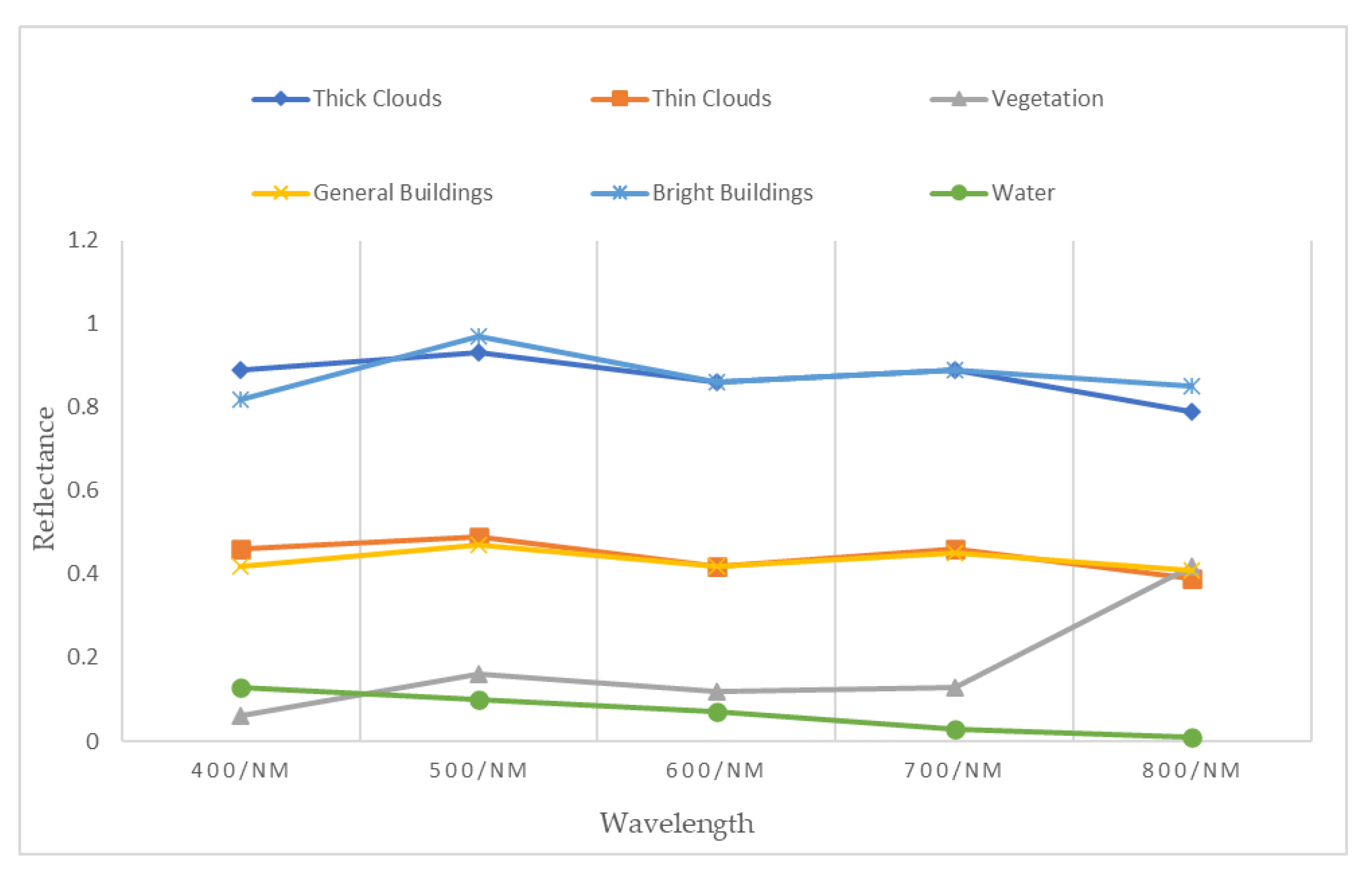
The spectral-contextual information of clouds and bright buildings in remote sensing images is very similar, as shown in Figure 1. Bright buildings in the images will cause accuracy of cloud detection methods based on spectral features to decrease. Therefore, how to distinguish between clouds and bright buildings in the images is one of the key factors to improve the accuracy of cloud detection.
In the visible bands and NIR band, clouds and bright buildings cannot be effectively distinguished by thresholds of a single band, but experiments have shown that the lower quartile of clouds in the blue band is larger than the upper quartile of the red band. There is little overlap between them. The corresponding bright buildings have large overlap in the upper and lower quartiles of the blue and red bands, and the lower quartile of the blue band is smaller than the upper quartile of the red band (Figure 2). The underlying surfaces are divided into water and non-water. The dynamic threshold can be set by the difference of the TOA reflectance, which could be used to distinguish between clouds and bright buildings in GF-6 WFV data. The specific equation is as follows:
In Equation (4), (Band1, 25) represents the lower quartile of the blue band and (Band3, 75) represents the upper quartile of the red band. The explanation for quartiles is that in statistics, all values are arranged from small to large and divided into four equal parts. It should be noted that “all values” here refers to all radiances of the potential cloud pixels identified in the above steps in a certain band. When calculating the upper and lower quartiles of band 1, “all values” is all radiances in the blue band, which is obtained by the potential cloud pixels identified in the detected image. Similarly, when calculating the upper and lower quartiles of band 3, “all values” is all radiances of the red band, which is obtained by the potential cloud pixels identified in the detected image. According to the arranged values, the values at the three division points from small to large are the lower quartile, median, and upper quartile. The lower quartile is the 25th percentile value and the upper quartile is the 75th percentile value after a set of data is arranged. In general, (Band1, 25) and (Band3, 75) are to take the 25th percentile value and 75th percentile value, which are ordered by each row of the blue and the red bands.
- 5.
- Stratus Test
As cloud base height can be any value from 200 meters to 12,000 meters [23], the base of fog is at the earth’s surface. Whether it is cloud or fog, the height relative to the ground will be affected by various factors such as humidity and temperature. Therefore, both cloud base height and fog base height are uncertain. The height relative to the ground alone is not enough to distinguish clouds from fog_W. The blue band in the visible band’s range has a larger scattering intensity and is most sensitive to fog, so it is often used to identify fog.
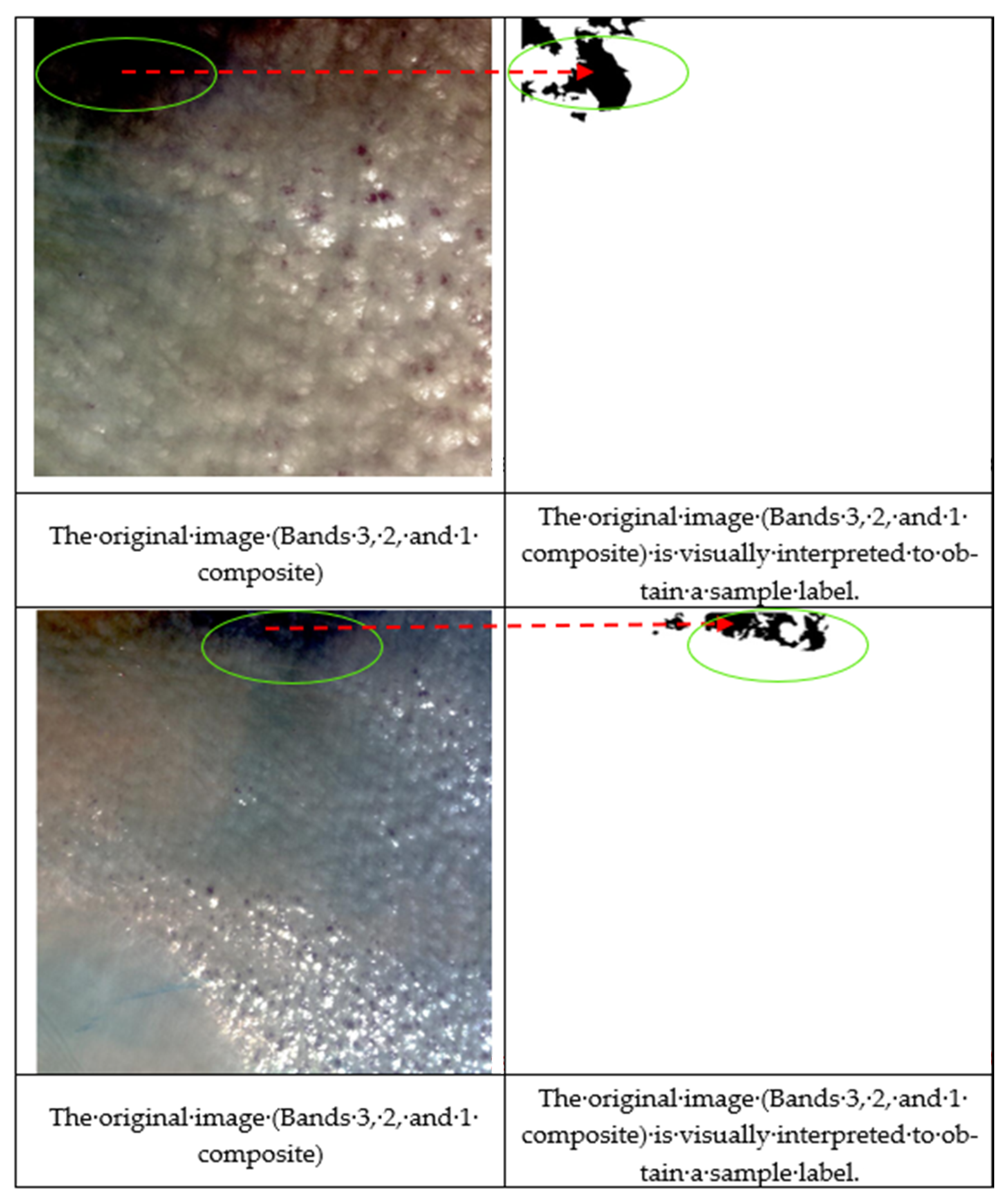
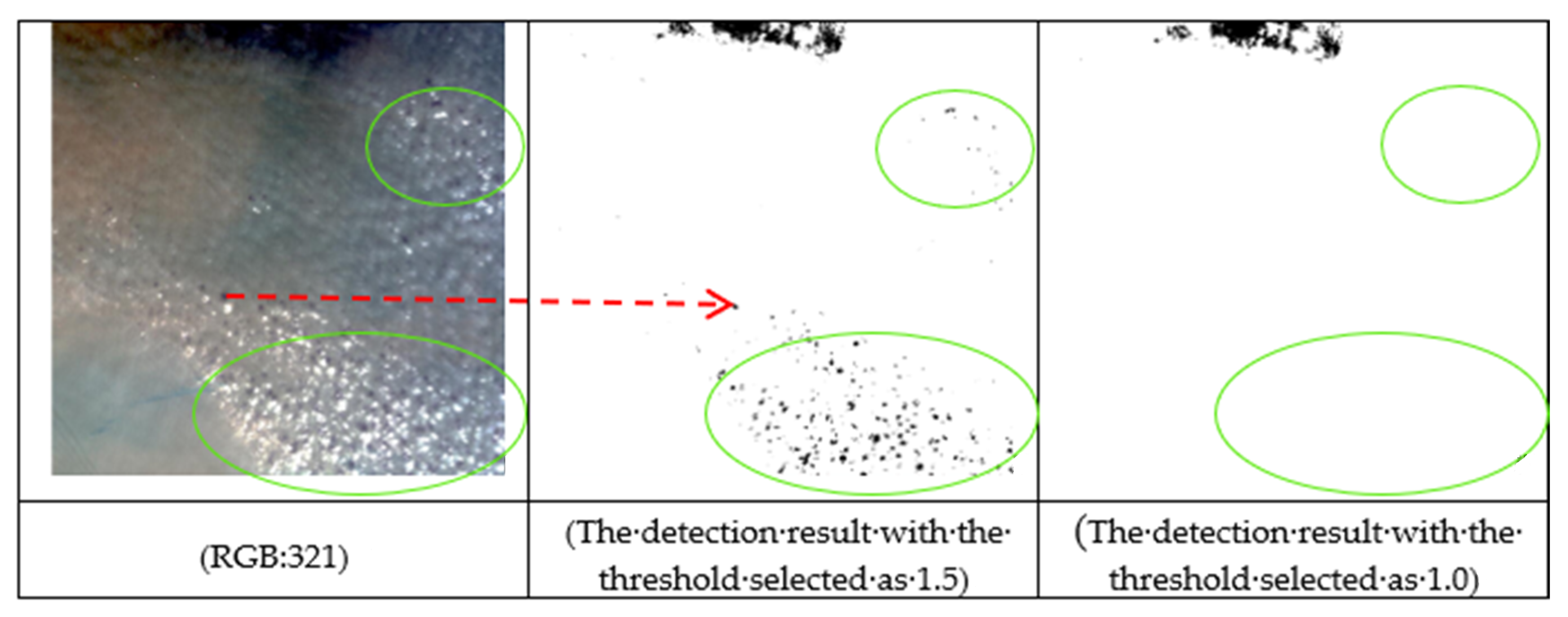
In the GF-6 WFV data, a scene with both stratus with high humidity and fog_W are selected, and stratus and fog_W are identified by visual interpretation. As shown in Figure 3, sample labels are obtained by artificial vectorization of the identified stratus and fog_W images. The experimental research in this paper shows that there is a large difference on the ratio of blue band to red edge position 1 band between stratus and fog_W at higher humidity levels. According to the trend lines of the ratio of stratus and fog_W in the blue and red edge position 1 band in Figure 4, the ratio of stratus over water falls in the interval between 1.0 and 4.4, and the ratio of fog_W falls near 1. There is a clear distinction between them. According to Figure 4, if we simply consider the fog_W, the lower limit of the threshold should indeed be increased. However, it is also necessary to consider thin clouds in the stratus with high humidity. The ratio of the blue band to red edge position 1 band of thin clouds is slightly higher than 1, but lower than 1.5. When the lower limit of the threshold is set to 1.5, as shown in Figure 5, according to the arrow pointing and the circled part, it can be seen that the thin clouds of the stratus with high humidity is difficult to identify.
Therefore, considering the stratus, thin clouds and fog_W, the specific equation is as follows:
2.2.3. Cloud Pixels Probability Calculation
- Cloud recognition is not an all-or-nothing state due to the complexity of clouds in remote sensing images. Therefore, the distribution of cloud pixels in remote sensing images can be further determined by calculating the cloud probability of PCPs to better identify clouds. Because water pixels and land pixels have high variability, the Fmask cloud detection algorithms of versions 3.2 and 4.0 are referred to calculate cloud probabilities for water pixels and land pixels, respectively. Cloud probability for water
In the Fmask version 3.2, the cloud probability for water (wCloud-Prod) is determined by the temperature probability (wTemperature_Prob) and Brightness_Prob. However, the existing bands in the GF-6 WFV data cannot meet the requirements of wTemperature_Prob and Brightness_Prob, so this part of this research has been modified to some extent. For the Brightness_Prob over water, water is generally dark, especially in SWIR band reflectance, and the existence of clouds over water can increase SWIR band reflectance greatly [23]. Brightness_Prob is normalized based on these two features in Fmask version 3.2. However, due to the limitation of the GF-6 WFV data, the SWIR band is replaced by the NIR band based on the similar band characteristics, as shown in Equation (6) [20]. In addition, for water areas, the absence of wTemperature_Prob has little effects on the cloud detection accuracy [34]. Therefore, wTemperature_Prob is ignored in this study.
- 1
- Brightness probability for water:
wCloud_Probis is calculated by Brightness_Prob for water:
Through the above detection, if the result is larger than 0.5, the water pixel is identified as a cloud pixel. This fixed threshold works well for detecting clouds over water [23].
- 2.
- Cloud probability for land
Land pixels have higher variability compared with water pixels. Since the calculation of the cloud probability for land (LCloud-Prob) in Fmask version 3.2 requires TIR band, LTemperature_Prob can no longer be calculated. Therefore, the improvement of the LTemperature_Prob by Qiu et al. (2019) is referred to. LCloud-Prob is a combination of variation probability (Variability-Prob) and the HOT-based cloud probability (LHOT) computed as follows:
- 1)
- LHOT:
In Equation (9), LHOT is the result of normalizing the HOT value based on the clear-sky pixels, and the constant 0.04 is the differential assumption for the clear-sky pixels HOT value [34]. LHOT is used as an alternative to LTemperature_Prob for GF-6 WFV data. According to the sensitivity analysis of the global cloud reference mask, the 17.5 and 82.5 percentiles are selected as the thresholds [23]. 17.5 and 82.5 percentiles are inherited from the Fmask version 3.2, which can provide the HOT interval for clear-sky land pixels [34]. The clear-sky land pixels are obtained after the identification of potential cloud pixels and the calculation of cloud probability for GF-6 WFV of each scene. Therefore, these two percentages are aimed at the HOT of the intermediate quantity (clear-sky land pixels) obtained during the detection process.
- 2)
- The variability probability for land:
In remote sensing images, land pixels contain richer information of features. Different features increase the variability of land pixels, making it difficult to find a definite normalized value. The Fmask cloud detection algorithm of version 3.2 uses NDVI, NDSI and “Whiteness” to capture cloud pixels in the visible bands and NIR band range. For GF-6 WFV data, the unusable index NDSI is removed, and the largest of the two indices is subtracted by 1 to satisfy the spectral variability as shown in Equation (10). Note the “whiteness” index was originally proposed by Gomez-Chova et al. (2007) [35]. Clouds often appear as white features due to the “flat” reflectivity in the visible bands. Therefore, the sum of the absolute difference between the visible bands and the overall brightness is used to capture this type of cloud property, which is “Whiteness”. The original “Whiteness” requires many narrow visible bands and is not suitable for Landsat sensors [23]. Therefore, Zhu et al. improved the “Whiteness” and only required three narrow visible bands to complete. By dividing the difference by the average value of the visible bands, the new “Whiteness” index works well for Landsat imagery and 0.7 (sensitivity analysis of the global cloud reference dataset) appears to be an optimal threshold for excluding clear-sky pixels that exhibit high variability in the visible bands [23]. In addition, the “Whiteness” threshold with the highest average cloud overall accuracy is the optimal threshold obtained by Zhu et al. based on 142 experimental images. The above “Whiteness” index is used to exclude pixels that are not “white” enough to be clouds [23]. However, it should be noted that the “Whiteness” does not completely exclude features such as bare soil and rocks that have “flat” reflectance in the visible bands. The “Whiteness Test” is also applicable to GF-6 WFV data.
When dealing with saturated pixels, the spectral variability based on NDVI may not be accurate [23]. In this case, the modified NDVI is used in Equation (10). The NDVI values are modified as follows: if a pixel is in the red band is saturated and has an NIR band larger than the red band, then Fmask provides a zero value for this pixel’s NDVI [23].
LCloud-Prob is calculated by combining both LHOT and Variability-Prob:
The threshold of clouds for land defined in Fmask version 3.2 is composed of a constant 0.2 based on sensitivity analysis and an upper limit of 82.5 percentile of the probability of a clear-sky land pixels, as shown in Equation (12). At this point, through the calculation of cloud probability and the PCPs identified in the previous step, Fmask generates potential cloud layers by Equation (13). In addition, if the value of LCloud_Prod exceeds 99%, Fmask will search for missing cloud pixels [23].
After the potential cloud layer is identified, Fmask version 3.2 spatially improves the cloud mask. If five or more pixels in the 3 × 3 neighborhood of a pixel are cloud pixels, the pixel is recognized as a cloud pixel; otherwise, it is recognized as a clear-sky pixel [23].
In addition, it is inevitable that there will be sporadic noise points in the results of cloud detection due to the complexity and variety of ground features and the presence of noise in the image. After using the improved Fmask algorithm to perform cloud detection on GF-6 data, the results are filtered through opening and closing to complete the post-processing of sporadic pixels and tiny holes in the image.
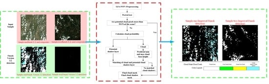
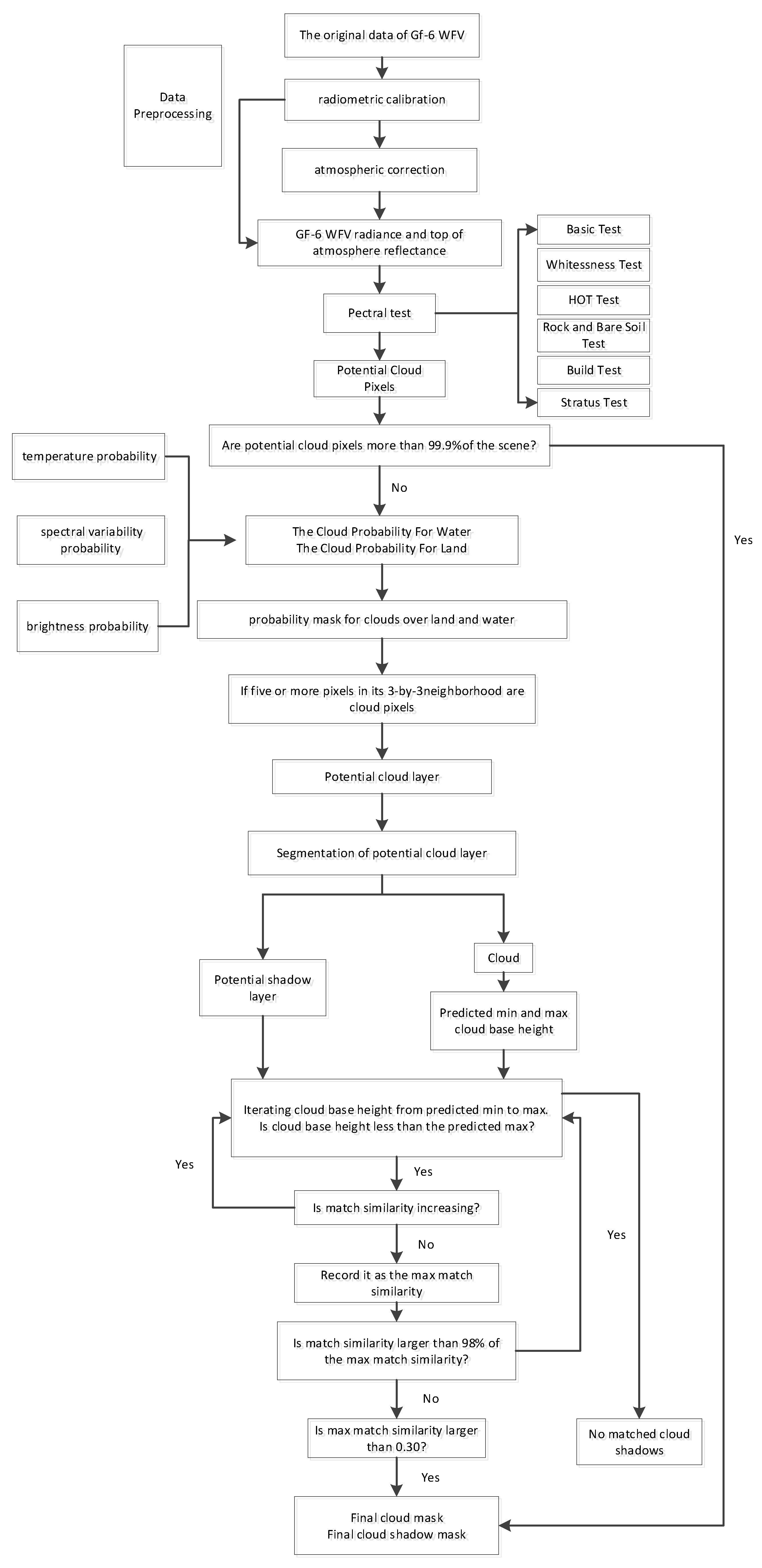
For the improved Fmask cloud detection algorithm, the flow chart is shown in Figure 6.
3. Results and Discussion
3.1. Experimental Results
This part is mainly divided into qualitative evaluation and quantitative evaluation of cloud detection results, in which the qualitative evaluation is compared and analyzed by visual interpretation. On the one hand, the results detected by the improved Fmask are compared and analyzed with real cloud images and the cloud detection results of Fmask version 3.2. On the other hand, the results of cloud detection using the improved Fmask are compared and analyzed with real cloud images and the cloud detection results of four traditional methods, such as OTSU, MMOTSU, SVM and K-means. Quantitative analysis is to intuitively evaluate the accuracy of cloud detection results of different methods through calculation of precision evaluation index by confusion matrix [10].
In this paper, multi scene images of different regions of GF-6 WFV data are selected for accuracy validation. In order to make the results more accurate and reliable, it is selected that images with different underlying surface such as vegetation, water, buildings and bare soil and containing various cloud types such as thick and thin clouds for detection. Representative sub-images are selected for the qualitative and quantitative analysis of the results due to the large size of the GF-6 WFV data.
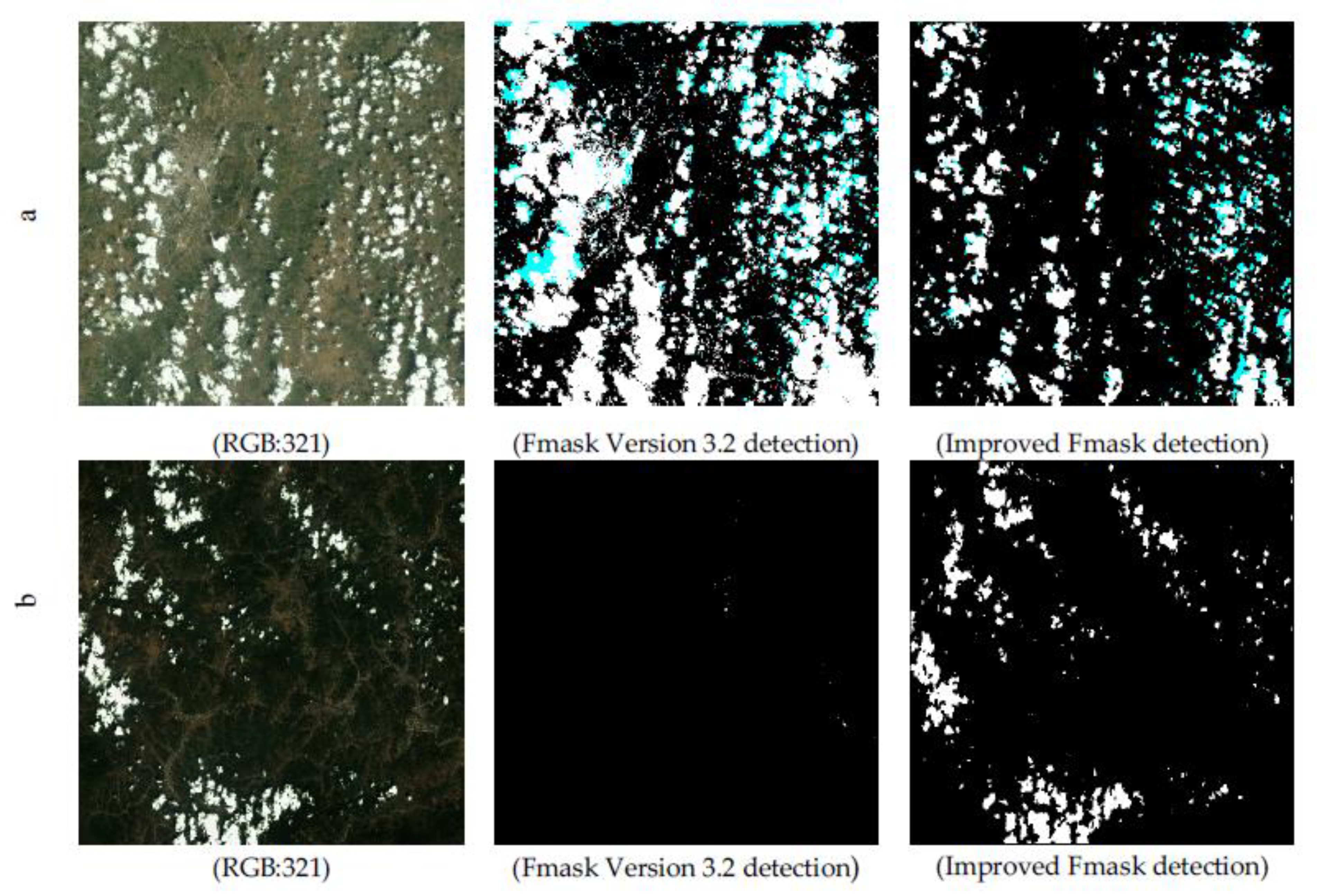
This research is improved on the basis of the Fmask version 3.2. The Fmask both of version 3.2 and the improved version are used to detect the representative subgraphs of GF-6 WFV data. In order to adapt to GF-6WFV data, Fmask version 3.2 mainly omitted the following parts: (1) SWIR, TIR and NDSI in "Basic Test" are all omitted, only NDVI is left due to the lack of TIR band and SWIR band in GF-6 WFV data. (2) "B4/B5 Test " is omitted because GF-6 WFV data lacks SWIR band. (3) The calculation of wTemperature_Prob, Brightness_Prob, and LTemperature_Prob are omitted, and the modified NDSI in the calculation of Variability-Prob is omitted due to the lack of SWIR band and TIR band in the GF-6WFV data. Those results are compared and analyzed, as shown in Figure 7. In Figure 7, the comparison shows that the Fmask version 3.2 has a large commission error of cloud detection, especially when the underlying surface is bright, which is easily identified as clouds. For thin clouds attached to the edges of thick clouds, the unimproved algorithm can be very sensitive, to the extent that serious misclassifications occur. Unimproved algorithms may cause serious commission errors because they are too sensitive. Overall, the results of the Fmask version 3.2 are relatively unstable, with a high omission errors and commission errors of clouds in the detection results. To address the above-mentioned problems of the Fmask version 3.2 for GF-6 WFV data cloud detection, the algorithm is improved, and the improved detection results are analyzed in this study.
3.2. Qualitative Analysis
3.2.1. Bright Building
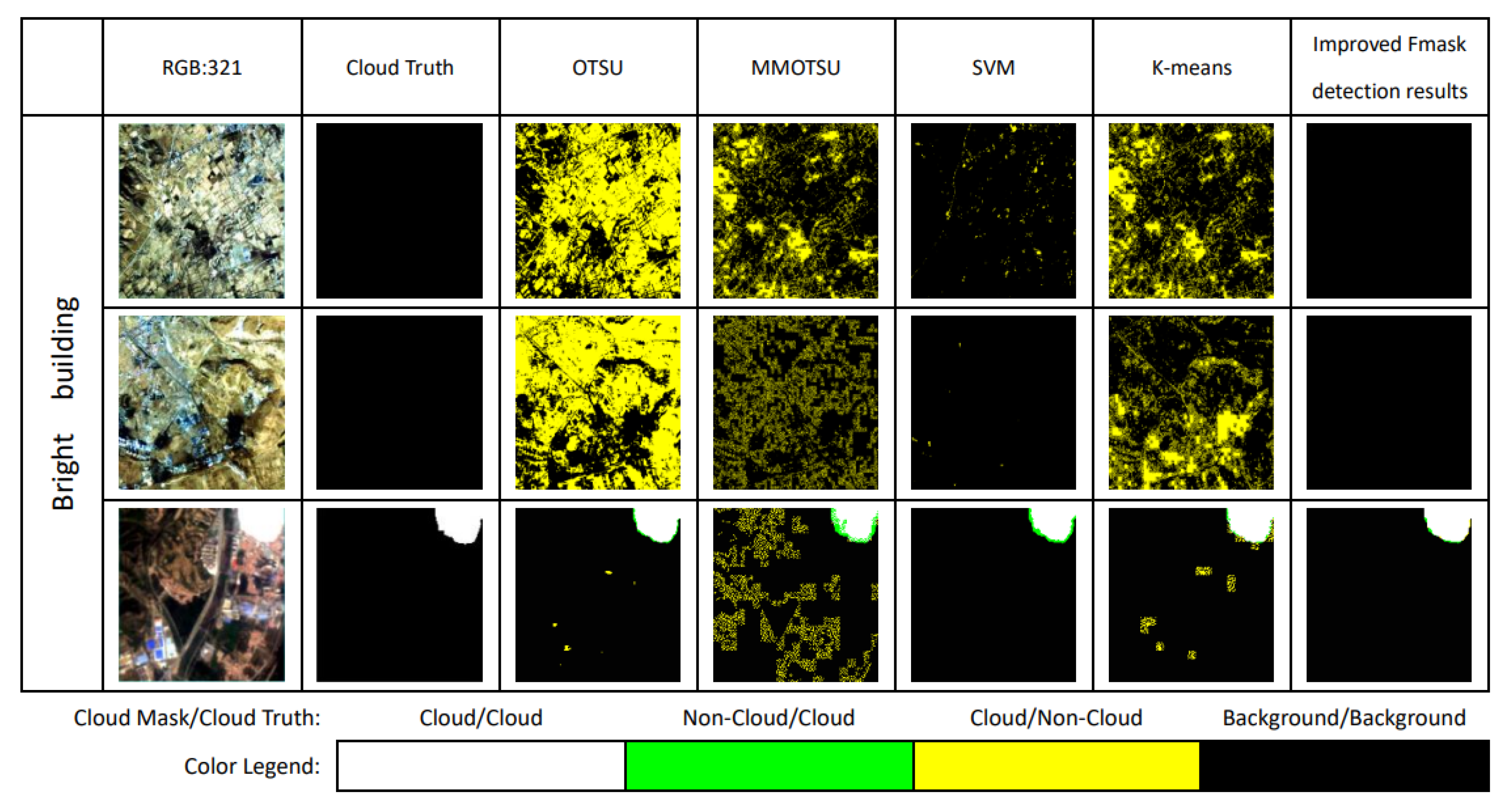
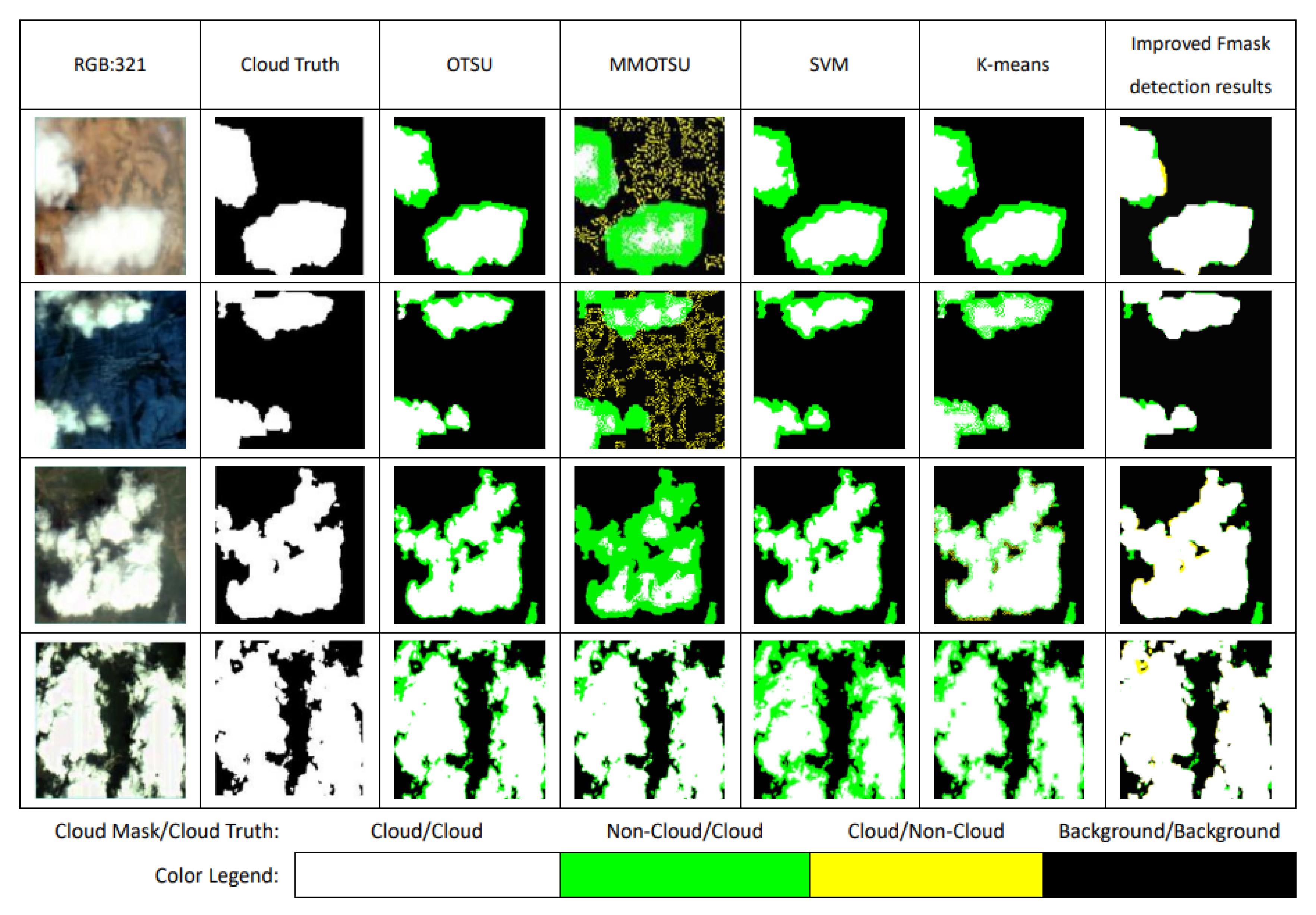
When the underlying surface of the detected object is a building with high reflectivity, its reflectivity is extremely similar to a cloud, which causes great interference in cloud detection. In Figure 8 each row from left to right are the RGB form of the original subgraph, the real cloud image, the results of the four traditional cloud detection methods of OTSU, MMOTSU, SVM, and K-means, and the result of cloud detection by improved Fmask. Among them, the yellow in the detection result is the commission errors and the green is the omission errors. In comparison, the cloud detection results of the four traditional methods of the images show high commission errors. Especially the OTSU, MMOTSU, and K-means methods, they have no resistance to images with large quantities of bright buildings. Additionally, the commission errors are extremely high, making the detection results unusable.
3.2.2. Water Surface
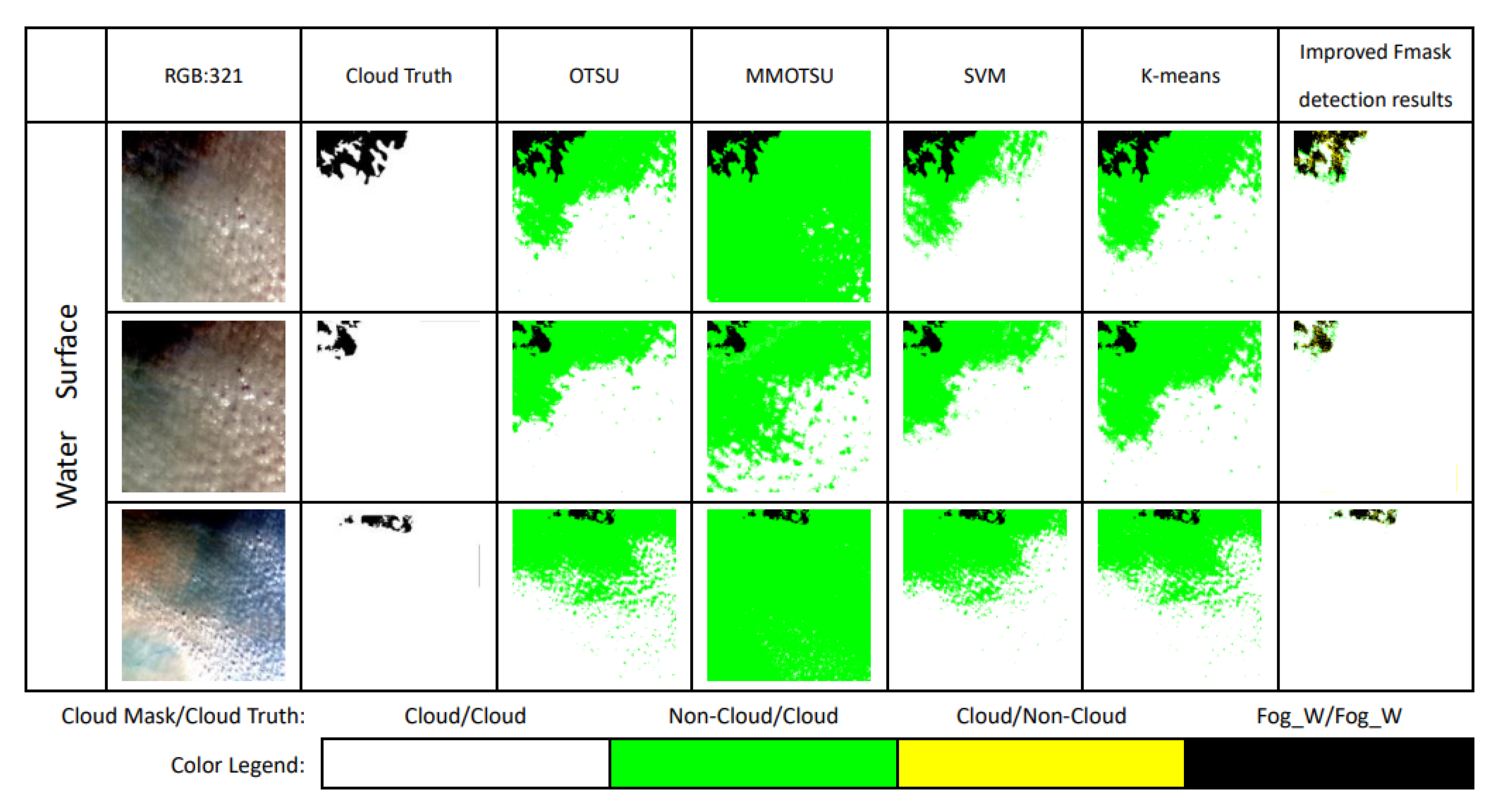
Conventional cloud detection algorithms such as OTSU have relatively high omission errors when detected objects are stratus with high humidity over water. The height of stratus relative to the water is reduced due to the high humidity, so that the height of stratus and fog_W cannot be used as a criterion to distinguish them from each other. In addition, the reflectivity of the high-humidity stratus cannot be solely used as a necessary condition for identifying due to it being lower than that of ordinary clouds. The improved Fmask uses the ratio of the blue band to the red edge position 1 band to identify the stratus with high humidity over water. On account to the higher scattering intensity of the blue band, this ratio is further used to distinguish between stratus and fog_W. This algorithm greatly reduces the omission errors of higher humidity stratus over water compared to traditional algorithms such as OTSU, which can respond effectively to this type of cloud. The rightmost column of Figure 9 shows the series of results of this study’s detection. However, it should be noted that this study only distinguishes between stratus over water and fog_W and does not distinguish between clouds and fog on land separately.
3.2.3. Cultivated Land, Woodland, Bare Soil
When the underlying surfaces of the images are cultivated land, woodland, or bare soil, the reflectance of bright ground surfaces, such as bright rocks, is more similar to clouds. This poses a challenge for cloud detection. The spectral reflection of different ground objects is in a mixed state and affect each other. The mixing of cloud pixels with bright surface pixels such as bare soil, rocks, etc. causes great interference in cloud detection, resulting in several traditional cloud detection algorithms having high commission errors. Experiments show that there are differences in the ratio of the green band to the red band between bright surfaces and clouds. Based on those features, the improved cloud detection algorithm of Fmask comprehensively considers the conditions of thick clouds and thin clouds, which sets corresponding thresholds to exclude the influence of bright ground surfaces such as rocks in cloud detection. The rightmost column of Figure 10 is the result of cloud detection by this research method. It can be seen from the comparison that this method is better than traditional cloud detection algorithms such as MMOTSU.
3.2.4. Others
Due to their low density, thin clouds are easily affected by the reflectivity of the underlying surface [36]. Whether it is a thin cloud attached to the edge of a thick cloud or a thin cloud that exists alone, it is easy to be mistaken for non-cloud pixels. In Figure 11, the detection results of traditional algorithms such as OTSU have high commission errors for thin clouds attached to the edge of thick clouds, which makes it difficult to extract these thin clouds effectively. In this study, we do not target the identification of thin clouds that exist alone, only improving the detection of thin clouds attached to the edges of thick clouds. Whether in the “Basic Test”, “HOT Test”, “Rock and Bare Soil Test”, or in the distinguishing stage of stratus with high humidity and fog_W, the factors of thick cloud, thin cloud and fog are comprehensively considered when setting the thresholds. In addition, according to the recognition results, the detected cloud pixels are buffered three pixels outward in eight directions. On the one hand, this can effectively fill the identification holes. On the other hand, it can further identify thin clouds at the edge of thick clouds.
Affected by the relatively narrow wavelength range covered by GF-6 WFV data, it is difficult for the Fmask algorithm to more effectively identify thin clouds alone. When there are a large number of thin clouds alone to be detected, the algorithm in this study still cannot reach the ideal detection accuracy.
3.3. Quantitative Analysis and Evaluation
In order to evaluate the algorithm more comprehensively and accurately, quantitative analysis and comparison are essential. Because the amount of GF-6WFV data is large, those subgraphs are selected which have different underlying surfaces (such as buildings, bare soil, woodland, cultivated land and water surface) and include thick clouds and thin clouds. Their detection results are quantitatively evaluated. The subgraphs are analyzed and verified for accuracy with confusion matrix.
In the confusion matrix, the columns represent the predicted category, and the rows represent the true attribution category of the data. In short, the confusion matrix is a 2*2 situation analysis table, including TP (True Positive), FN (False Negative), FP (False Positive), and TN (True Negative). This chapter analyses the accuracy of cloud detection results with the help of TPR (True Positive Rate), PPV (Positive Predictive Value), TNR (True Negative Rate), and F1 Score (Harmonic average of Precision and Recall), which are calculated as follows.
With the help of ENVI, the vectorization process of the true color composite images (Bands 3, 2, and 1 composite) is carried out. The results of the vectorization process are used as the sample true classification labels of the confusion matrix, and the results of the detection using OTSU, MMOTSU, K-means, SVM and the improved Fmask cloud detection algorithm in this paper are used as the predicted classification results of the confusion matrix. According to Equations (14)–(17), the accuracy evaluation indices of the detection results from different detection methods are calculated to obtain Table 2.
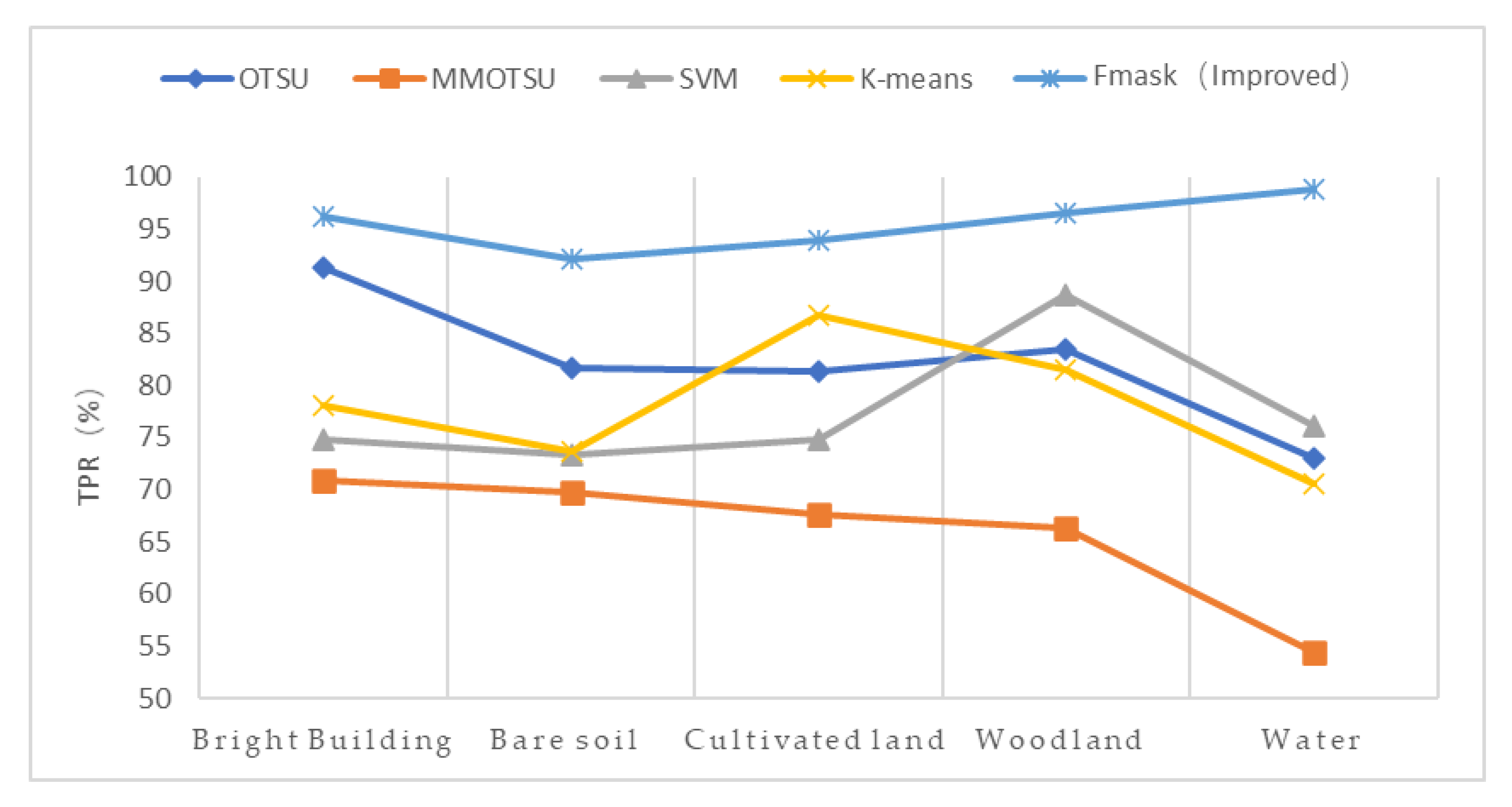
It can be seen from Table 2 that the improved Fmask cloud detection algorithm has higher TPR in the detection results. For the cloud pixels, the average TPR of the improved Fmask can reach 95.51%, compared with 82.19% of OTSU, 65.84% of MMOTSU, 77.57% of SVM, and 78.14% of K-means. Among them, when the research object is stratus with high humidity over water, the TPR of the improved Fmask reaches 98.80%, which significantly improves the usability of the image. When the underlying surfaces contain more bright buildings, it is obvious that the improved Fmask has achieved a better effect whether it is TPR or TNR. In addition, when the underlying surface contains bare soil and rock and other bright surfaces, the improved Fmask adds the process of “Rock and Bare Soil Test” for this type of images in the spectral test, which improves the TPR. However, because this study did not fundamentally solve the problem of thin clouds, the improved Fmask has relatively high commission errors when there are many independent thin clouds in the images. Under the premise of comprehensively considering the TPR and PPV, the F1-Score of the improved Fmask for different underlying surfaces, such as buildings and woodlands, exceeds 95.00%. When the underlying surfaces are cultivated land, the F1-Score of the improved Fmask reaches 99.66%. When the detected object is stratus with high humidity over water, the F1-Score is 89.22%, caused by the high omission errors of cloud pixels. However, it is still higher than the comparable algorithms, such as OTSU.
The TPR obtained by different methods is analyzed separately, as shown in Figure 12. According to the line chart, it can be clearly seen that the TPR detected by the improved Fmask is higher than other traditional methods, and the detection results for different types of underlying surfaces are relatively sfigure. When the research object is stratus with high humidity over water, the improved Fmask cloud detection algorithm has obvious advantages and high usability.
4. Conclusions
This research improves the Fmask version 3.2 based on the GF6-WFV data. The improved parts are mainly focused on the spectral-contextual information and probability calculation, which are divided into six aspects. First, in response to the problem that the GF-6 WFV data does not have bands required for the "Basic Test" in the Fmask version 3.2, the consideration of the multispectral remote sensing data and the available bands are added. The detection is replaced with a combination of NDVI inherited from the Fmask version 3.2 and blue band to complete the distinction between PCPs and typical features such as vegetation. Second, the comprehensive consideration of fog and thin clouds for the “HOT Test” in the improved Fmask is added. The threshold in the Fmask version 3.2 is modified to better distinguish between thin clouds and fog. Third, the ratio of the green band to the NIR band is used for the underlying surfaces with bare soil and rock to reduce the commission errors. Fourth, for bright buildings, the relationship between the upper and lower quartiles of the blue and red bands is used to increase TPR, so as to reduce the commission errors of bright building images. Fifth, for stratus with high humidity, the blue band and red edge position 1 band are combined to identify and distinguish stratus from fog_W, which increases the detection of fog_W and stratus with high humidity and significantly reduces the omission errors of stratus. Sixth, the land temperature probability is replaced by the HOT-based cloud probability (LHOT), and SWIR in brightness probability for water is replaced by NIR. The improved Fmask is used to detect GF-6 WFV data and evaluate the accuracy of the results by qualitative and quantitative methods. Comparing the results of different detection methods with the results of visual interpretation of GF-6 WFV data, the results of cloud detection are qualitatively verified. The experiment results show that the improved Fmask can achieve better detection compared with traditional cloud detection algorithms such as OTSU, MMOTSU, SVM, and K-means. The accuracy of the detection results of traditional methods, such as OTSU and the improved Fmask method, is evaluated with the aid of the confusion matrix. Through the analysis of the quantitative evaluation results, it can be seen that the average TPR of the improved Fmask for GF-6 WFV data can reach 95.51%, which is better than the 82.19% of OTSU, 65.84% of multi-threshold OTSU, 77.57% of SVM, and 78.14% of K-means under the same conditions. The improved Fmask achieves a 6.26% omission error for clear-sky pixels. The omission errors of stratus with high humidity are relatively high but can be controlled within the effective extraction range of cloud pixels.
For GF-6 WFV data, the improved Fmask still has the following problems.
- No snow and ice regions are detected in this study since the lack of snow and ice regions in the GF-6 WFV data;
- There is inevitably some bias in the process of accuracy evaluation caused by some subjective human vectorization, because the real vectorized cloud images are obtained by manual vectorization with the help of visual interpretation;
- The effective band for detecting thin clouds is not explored due to the narrow wavelength range covered by GF-6 WFV data; particularly, a poor detection results when there are more thin clouds alone in the image.
To address the problems of the improved Fmask algorithm detection results, the following work still needs to be conducted.
- A simple distinction between clouds and snow can be made if snow and ice areas appear in the subsequent GF-6 WFV data, although the data do not contain SWIR bands that can be used for snow and ice detection. The distinction is performed that clouds and cloud shadows are present in pairs while snow exists alone;
- For thin clouds that exist alone, detection can be attempted by the combination of improved Fmask algorithm and spatial texture features.
Author Contributions
X.Y. proposed the idea, implemented the methodology and wrote the manuscript. L.S. and B.A. contributed to improving the methodology, and B.A. acted as the corresponding author. X.T., H.X. and Z.W. helped to edit and improve the manuscript. All authors have read and agreed to the published version of the manuscript.
Funding
This work was jointly supported by the National Natural Science Foundation of China [Grant No. 62071279, 41930535], the SDUST Research Fund [Grant No. 2019TDJH103], and the Major Science and Technology Innovation Projects of Shandong Province (2019JZZY020103).
Data Availability Statement
The data are not publicly available due to restrictions privacy.
Acknowledgments
The authors would like to thank Land Satellite Remote Sensing Application Center for providing the GF-6 WFV data.
Conflicts of Interest
The authors declare no conflict of interest.
References
- Xiang, P.S. A Cloud Detection Algorithm for MODIS Images Combining Kmeans Clustering and Otsu Method. In Proceedings of the IOP Conference Series: Materials Science and Engineering; IOP Publishing: Bristol, UK, 2018; Volume 6, p. 62199. [Google Scholar]
- Dan, L.P.; Mateo-García, G.; Gómez-Chova, L. Benchmarking Deep Learning Models for Cloud Detection in Landsat-8 and Sentinel-2 Images. Remote. Sens. 2021, 13, 992. [Google Scholar]
- Lu, C.L.; Bai, Z.G.; Li, Y.C.; Wu, B.; Di, G.D.; Dou, Y.F. Technical Characteristic and New Mode Applications of GF-6 Satellite. Spaceraft Eng. 2021, 30, 7–14. [Google Scholar]
- Yao, J.Q.; Chen, J.Y.; Chen, Y.; Liu, C.Z.; Li, G.Y. Cloud detection of remote sensing images based on deep learning and condition random field. Sci. Surv. Mapp. 2019, 44, 121–127. [Google Scholar]
- Wu, Y.J.; Fang, S.B.; Xu, Y.; Wang, L.; Li, X.; Pei, Z.F.; Wu, D. Analyzing the Probability of Acquiring Cloud-Free Imagery in China with AVHRR Cloud Mask Data. Atmosphere 2021, 12, 214. [Google Scholar] [CrossRef]
- Sun, L.; Wei, J.; Wang, J.; Mi, X.T.; Guo, Y.; Lv, Y.; Yang, Y.K.; Gan, P.; Zhou, X.Y.; Jia, C.; et al. A Universal Dynamic Threshold Cloud Detection Algorithm (UDTCDA) supported by a prior surface reflectance database. J. Geophys. Res. Atmos. 2016, 121, 7172–7196. [Google Scholar] [CrossRef]
- Lu, Y.H. Research on Automatic Cloud Detection Method for Remotely Sensed Satellite Imagery with High Resolution. Master’s Thesis, Xidian University, Xi’an, China, 2018. Unpublished work. [Google Scholar]
- Mao, F.Y.; Duan, M.M.; Min, Q.L.; Gong, W.; Pan, Z.X.; Liu, G.Y. Investigating the Impact of Haze on MODIS Cloud Detection; John Wiley & Sons, Ltd.: Hoboken, NJ, USA, 2015; Volume 120, pp. 237–247. [Google Scholar]
- Shin, D.; Pollard, J.K.; Muller, J.P. Cloud detection from thermal infrared images using a segmentation technique. Int. J. Remote. Sens. 1996, 17, 2845–2856. [Google Scholar] [CrossRef]
- Li, Z.W.; Shen, H.F.; Li, H.F.; Xia, G.S.; Gamba, P.; Zhang, L.P. Multi-feature combined cloud and cloud shadow detection in GaoFen-1 wide field of view imagery. Remote Sens. Environ. 2017, 191, 342–358. [Google Scholar] [CrossRef] [Green Version]
- Fisher, A. Cloud and Cloud-Shadow Detection in SPOT5 HRG Imagery with Automated Morphological Feature Extraction. Remote Sens. 2014, 6, 776–800. [Google Scholar] [CrossRef] [Green Version]
- Gesell, G. An algorithm for snow and ice detection using AVHRR data an extension to the APOLLO software package. Int. J. Remote Sens. 1989, 10, 897–905. [Google Scholar] [CrossRef]
- Jia, L.L.; Wang, X.Q.; Wang, F. Cloud Detection Based on Band Operation Texture Feature for GF-1 Multispectral Data. Remote Sens. Inf. 2018, 33, 62–68. [Google Scholar]
- Wu, T.; Hu, X.Y.; Zhang, Y.; Zhang, L.L.; Tao, P.J.; Lu, L.P. Automatic cloud detection for high resolution satellite stereo images and its application in terrain extraction. ISPRS J. Photogramm. Remote Sens. 2016, 121, 143–156. [Google Scholar] [CrossRef]
- Cao, Q.; Zheng, H.; Li, X.S. A Method for Detecting Cloud in Satellite Remote Sensing Image Based on Texture. Acta Aeronaut. Astronaut. Sin. 2007, 28, 661–666. [Google Scholar]
- Vermote, E.; Saleous, N. LEDAPS Surface Reflectance Product Description; University of Maryland: City of College Park, MD, USA, 2007. [Google Scholar]
- Li, P.F.; Dong, L.M.; Xiao, H.C.; Xu, M.L. A cloud image detection method based on SVM vector machine. Neurocomputing 2015, 169, 34–42. [Google Scholar] [CrossRef]
- Tan, K.; Zhang, Y.J.; Tong, X. Cloud Extraction from Chinese High Resolution Satellite Imagery by Probabilistic Latent Semantic Analysis and Object-Based Machine Learning. Multidiscip. Digit. Publ. Inst. 2016, 8, 963. [Google Scholar] [CrossRef] [Green Version]
- Li, Z.W.; Shen, H.F.; Cheng, Q.; Liu, Y.H.; You, S.C.; He, Z.Y. Deep learning based cloud detection for medium and high resolution remote sensing images of different sensors. ISPRS J. Photogramm. Remote Sens. 2019, 150, 197–212. [Google Scholar] [CrossRef] [Green Version]
- Liu, X.Y.; Sun, L.; Yang, Y.K.; Zhou, X.Y.; Wang, Q.; Chen, T.T. Cloud and Cloud Shadow Detection Algorithm for Gaofen-4 Satellite Data. Acta Opt. Sin. 2019, 39, 438–449. [Google Scholar]
- Irish, R.R.; Barker, J.L.; Goward, S.N.; Arvidson, T. Characterization of Landsat-7 ETM+ automated cloud-cover assessment (ACCA) algorithm. Photogramm. Eng. Remote Sens. 2006, 72, 1179–1188. [Google Scholar] [CrossRef]
- Irish, R.R. Landsat 7 automatic cloud cover assessment. SPIE Def. Commer. Sens. 2000, 4049, 348–355. [Google Scholar]
- Zhu, Z.; Woodcock, C.E. Object-based cloud and cloud shadow detection in landsat imagery. Remote Sens. Environ. 2012, 118, 83–94. [Google Scholar] [CrossRef]
- Frantz, D.; Haß, E.; Uhl, A.; Stoffels, J.; Hill, J. Improvement of the Fmask algorithm for Sentinel-2 images: Separating clouds from bright surfaces based on parallax effects. Remote Sens. Environ. 2018, 215, 471–481. [Google Scholar] [CrossRef]
- Huang, Y. Cloud Detection of Remote Sensing Images Based on Saliency Analysis and Multi-texture Features. Master’s Thesis, Wuhan University, Wuhan, China, 2019. Unpublished work. [Google Scholar]
- Wieland, M.; Li, Y.; Martinis, S. Multi-sensor cloud and cloud shadow segmentation with a convolutional neural network. Remote Sens. Environ. 2019, 230, 11203. [Google Scholar] [CrossRef]
- Li, X.; Zheng, H.; Han, C.; Zheng, W.; Chen, H.; Jing, Y.; Dong, K. SFRS-Net: A Cloud-Detection Method Based on Deep Convolutional Neural Networks for GF-1 Remote-Sensing Images. Remote Sens. 2021, 13, 2910. [Google Scholar] [CrossRef]
- Wang, H.; Wang, Y.; Wang, Y.; Qian, Y. Cloud Detection of Landsat Image Based on MS-UNet. Prog. Laser Optoelectron. 2021, 58, 87–94. [Google Scholar]
- Cilli, R.; Monaco, A.; Amoroso, N.; Tateo, A.; Tangaro, S.; Bellotti, R. Machine Learning for Cloud Detection of Globally Distributed Sentinel-2 Images. Remote Sens. 2020, 12, 2355. [Google Scholar] [CrossRef]
- Dong, Z.; Sun, L.; Liu, X.R.; Wang, Y.J.; Liang, T.C. CDAG-Improved Algorithm and Its Application to GF-6 WFV Data Cloud Detection. Acta Opt. Sin. 2020, 40, 143–152. [Google Scholar]
- Wang, Y.J.; Ming, Y.F.; Liang, T.C.; Zhou, X.Y.; Jia, C.; Wang, Q. GF-6 WFV Data Cloud Detection Based on Improved LCCD Algorithm. Acta Opt. Sin. 2020, 40, 169–180. [Google Scholar]
- Jiang, M.M.; Shao, Z.F. Advanced algorithm of PCA-based Fmask cloud detection. Sci. Surv. Mapp. 2015, 40, 150–154. [Google Scholar]
- Zhu, Z.; Wang, S.; Woodcock, C.E. Improvement and expansion of the Fmask algorithm: Cloud, cloud shadow, and snow detection for Landsats 4–7, 8, and Sentinel 2 images. Remote Sens. Environ. 2015, 159, 269–277. [Google Scholar] [CrossRef]
- Qiu, S.; Zhu, Z.; He, B. Fmask 4.0: Improved cloud and cloud shadow detection in Landsats 4-8 and Sentinel-2 imagery. Remote Sens. of Environ. 2019, 231, 11205. [Google Scholar] [CrossRef]
- Gomez-Chova, L.; Camps-Valls, G.; Calpe-Maravilla, J.; Guanter, L.; Moreno, J. Cloud-Screening Algorithm for ENVISAT/MERIS Multispectral Images. IEEE Trans. Geosci. Remote Sens. 2007, 45, 4105–4118. [Google Scholar] [CrossRef]
- Sun, L.; Liu, X.Y.; Yang, Y.K.; Chen, T.T.; Wang, Q.; Zhou, X.Y. A cloud shadow detection method combined with cloud height iteration and spectral analysis for Landsat 8 OLI data. ISPRS J. Photogramm. Remote. Sens. 2018, 138, 197–203. [Google Scholar] [CrossRef]
Figure 1.
Spectral-contextual information of different typical objects in reflectance bands.

Figure 2.
Boxplots of band 1 and band 3 radiances for clouds and various surfaces.

Figure 3.
The comparison between the original images (Bands 3, 2, and 1 composite) and sample labels obtained by manual vectorization with the help of visual interpretation. Visual interpretation will vectorize the original images into clouds (white) and fog_W (black). The black circled in green is the fog_W recognized by visual interpretation.

Figure 4.
For GF-6 WFV data, the ratio of fog_W and stratus with high humidity over water in the blue band to the red edge position 1 band.
Figure 4.
For GF-6 WFV data, the ratio of fog_W and stratus with high humidity over water in the blue band to the red edge position 1 band.

Figure 5.
Comparison of results of different thresholds. The tail of the red arrow is the thin clouds in the image (Bands 3, 2, and 1 composite), and the head is the recognition of the corresponding part of the tail after the threshold of the ratio of the blue band to the red edge 1 band is increased to 1.5. The green circled is the recognition of thin clouds because of the different thresholds.

Figure 6.
Flow chart of the improved Fmask algorithm for GF-6WFV data cloud detection.

Figure 7.
Comparison of detection results between Fmask version 3.2 and the improved Fmask algorithm. (a) (Bands 3, 2, and 1 composite) and (b) (Bands 3, 2, and 1 composite) are images of different regions of GF-6 WFV data, respectively (The first image in each row). The second and third images in each row show the results of testing the same data by Fmask vesion 3.2 and improved Fmask. The white represents the detected cloud, the black represents the background, and the blue represents the detected cloud shadow.

Figure 8.
Comparison of the results of different cloud detection methods for images of bright building on the underlying surface. The first image in each row shows a subset of GF-6 WFV data (Bands 3, 2, and 1 composite). The second image in each row shows the distinction of the first image into cloud (white) and background (black) through visual interpretation. The third to seventh pictures in each row show the results of testing the same data by different methods, such as OTSU. Among them, the yellow represents what was actually non-cloud but was detected as cloud (commission errors), and the green represents what was actually cloud but was detected as non-cloud (omission errors).

Figure 9.
Comparison of detection results of different methods for high-humidity fog and stratus over water.
Figure 9.
Comparison of detection results of different methods for high-humidity fog and stratus over water.

Figure 10.
Compare the results of different cloud detection methods on images of cultivated land, woodland and bare soil with bright surfaces.
Figure 10.
Compare the results of different cloud detection methods on images of cultivated land, woodland and bare soil with bright surfaces.

Figure 11.
Comparison of the results of different cloud detection methods for thin clouds attached to the edge of thick clouds.Therefore, the improved Fmask cloud detection algorithm has a better recognition effect on thin clouds attached to the edge of thick clouds and reduces the commission errors of clouds. As shown in the rightmost column of Figure 11, the green color is significantly reduced, improving the overall accuracy of cloud detection.

Figure 12.
Comparison of the TPR of detecting cloud pixels by different methods.


Table 1.
GF-6 image data band information.
| Bands | Wavelength/µm | Fwhm/µm | Gains/(W/(m2. Sr µm)) | Offset/(W/(m2. Sr µm)) |
|---|---|---|---|---|
| Band1 | 0.45-0.52 | 0.07 | 0.0667 | 0.0 |
| Band2 | 0.52-0.59 | 0.07 | 0.0517 | 0.0 |
| Band3 | 0.63-0.69 | 0.06 | 0.0485 | 0.0 |
| Band4 | 0.77-0.89 | 0.12 | 0.0298 | 0.0 |
| Band5 | 0.69-0.73 | 0.04 | 0.0530 | 0.0 |
| Band6 | 0.73-0.77 | 0.04 | 0.0445 | 0.0 |
| Band7 | 0.40-0.45 | 0.05 | 0.0814 | 0.0 |
| Band8 | 0.59-0.63 | 0.04 | 0.0559 | 0.0 |
Table 2.
Comparison of accuracy evaluation of cloud detection results with different methods.
| Bright Building | Detection method | TPR/% | PPV/% | TNR/% | F1 Score/% |
| OTSU | 91.37 | 79.33 | 87.43 | 84.93 | |
| MMOTSU | 70.90 | 87.00 | 78.70 | 78.13 | |
| SVM | 74.80 | 100.00 | 100.00 | 85.58 | |
| K_MEANS | 78.17 | 91.00 | 67.97 | 84.10 | |
| FMASK(Improved) | 96.27 | 99.67 | 100.00 | 97.94 | |
| Woodland | OTSU | 83.40 | 100 | 100.00 | 90.95 |
| MMOTSU | 66.33 | 97.00 | 95.83 | 77.36 | |
| SVM | 88.67 | 99.00 | 98.97 | 93.55 | |
| K_MEANS | 81.57 | 99.00 | 98.87 | 89.44 | |
| FMASK(Improved) | 96.60 | 94.37 | 94.53 | 95.47 | |
| Cultivated land | OTSU | 81.37 | 100.00 | 100.00 | 89.73 |
| MMOTSU | 67.70 | 94.00 | 90.60 | 78.71 | |
| SVM | 74.87 | 100.00 | 100.00 | 85.63 | |
| K_MEANS | 86.67 | 99.67 | 99.60 | 92.72 | |
| FMASK(Improved) | 93.83 | 99.67 | 99.67 | 99.66 | |
| Bare Soil | OTSU | 81.73 | 100.00 | 100.00 | 89.95 |
| MMOTSU | 69.77 | 81.33 | 71.17 | 75.11 | |
| SVM | 73.40 | 100.00 | 100.00 | 84.66 | |
| K_MEANS | 73.73 | 99.00 | 98.90 | 84.52 | |
| FMASK(Improved) | 92.07 | 99.67 | 99.63 | 95.72 | |
| Water | OTSU | 73.10 | 98.33 | 97.73 | 83.86 |
| MMOTSU | 54.50 | 98.33 | 96.60 | 70.13 | |
| SVM | 76.10 | 98.33 | 97.73 | 85.80 | |
| K_MEANS | 70.57 | 98.33 | 97.27 | 82.17 | |
| FMASK(improved) | 98.80 | 81.33 | 84.17 | 89.22 |
Publisher’s Note: MDPI stays neutral with regard to jurisdictional claims in published maps and institutional affiliations. |
© 2021 by the authors. Licensee MDPI, Basel, Switzerland. This article is an open access article distributed under the terms and conditions of the Creative Commons Attribution (CC BY) license (https://creativecommons.org/licenses/by/4.0/).
Share and Cite
MDPI and ACS Style
Yang, X.; Sun, L.; Tang, X.; Ai, B.; Xu, H.; Wen, Z. An Improved Fmask Method for Cloud Detection in GF-6 WFV Based on Spectral-Contextual Information. Remote Sens. 2021, 13, 4936. https://0-doi-org.brum.beds.ac.uk/10.3390/rs13234936
AMA Style
Yang X, Sun L, Tang X, Ai B, Xu H, Wen Z. An Improved Fmask Method for Cloud Detection in GF-6 WFV Based on Spectral-Contextual Information. Remote Sensing. 2021; 13(23):4936. https://0-doi-org.brum.beds.ac.uk/10.3390/rs13234936
Chicago/Turabian StyleYang, Xiaomeng, Lin Sun, Xinming Tang, Bo Ai, Hanwen Xu, and Zhen Wen. 2021. "An Improved Fmask Method for Cloud Detection in GF-6 WFV Based on Spectral-Contextual Information" Remote Sensing 13, no. 23: 4936. https://0-doi-org.brum.beds.ac.uk/10.3390/rs13234936
Note that from the first issue of 2016, this journal uses article numbers instead of page numbers. See further details here.