Change Detection of Selective Logging in the Brazilian Amazon Using X-Band SAR Data and Pre-Trained Convolutional Neural Networks

Abstract

It is estimated that, in the Brazilian Amazon, forest degradation contributes three times more than deforestation for the loss of gross above-ground biomass. Degradation, in particular those caused by selective logging, result in features whose detection is a challenge to remote sensing, due to its size, space configuration, and geographical distribution. From the available remote sensing technologies, SAR data allow monitoring even during adverse atmospheric conditions. The aim of this study was to test different pre-trained models of Convolutional Neural Networks (CNNs) for change detection associated with forest degradation in bitemporal products obtained from a pair of SAR COSMO-SkyMed images acquired before and after logging in the Jamari National Forest. This area contains areas of legal and illegal logging, and to test the influence of the speckle effect on the result of this classification by applying the classification methodology on previously filtered and unfiltered images, comparing the results. A method of cluster detections was also presented, based on density-based spatial clustering of applications with noise (DBSCAN), which would make it possible, for example, to guide inspection actions and allow the calculation of the intensity of exploitation (IEX). Although the differences between the tested models were in the order of less than 5%, the tests on the RGB composition (where R = coefficient of variation; G = minimum values; and B = gradient) presented a slightly better performance compared to the others in terms of the number of correct classifications for selective logging, in particular using the model Painters (accuracy = 92%) even in the generalization tests, which presented an overall accuracy of 87%, and in the test on RGB from the unfiltered image pair (accuracy of 90%). These results indicate that multitemporal X-band SAR data have the potential for monitoring selective logging in tropical forests, especially in combination with CNN techniques.

1. Introduction

Land use, land use changes, and forests have historically been the sectors that most contribute to greenhouse gas emissions in Brazil, according to the Greenhouse Gas Emissions and Removal Estimates System—SEEG [1]. Therefore, the necessary containment of the increase in emissions is closely related to the control and combat of deforestation and forest degradation. Brazil has a robust system for monitoring and quantifying annual deforestation carried out by the National Institute for Space Research, called PRODES [2], and also a near-real time system of deforestation and degradation alerts, aimed at monitoring actions, called DETER-B [3]. In addition to these governmental systems, scientists and non-governmental organizations have proposed new operational methods aimed at detecting, mapping, and monitoring deforestation in tropical regions through different techniques and sensors [4,5,6,7].

Despite being widely explored for deforestation mapping, the application of remote sensing to monitor forest degradation still requires advances, especially due to the complexity of the nature of these processes [8]. Some studies show that emissions and the area impacted by forest degradation are underestimated [9] and exceed those by deforestation [10,11], and therefore should be incorporated in greenhouse gas emission reduction agreements [12]. Forest degradation includes forest fires, selective logging, drought, or any other event that results in the partial removal of forest cover [11]. Bullock and Woodcock [13] showed that in the Amazon forest, emissions from degradation are greater in dry periods and that approximately 30% of the carbon loss related to the forest comes from degradation. Several studies address the use of optical data for this purpose, especially Landsat satellite images, which provide a wide temporal coverage and the possibility of detecting forest disturbances through methods such as vegetation indices and spectral mixture analysis [14,15]. Multi-temporal very high-resolution satellite data, such as from WorldView-2 (0.5 m), have also been assessed to detect selective logging in tropical forests with moderate accuracy (64%) using machine learning Random Forest model [16]. These approaches, however, suffer from issues that are difficult to control, such as phenology and shadow variability in the imagery due to different periods of acquisition and view-geometry illumination interactions. Another limitation of the use of VHR images is its high cost, however, the high spatial resolution is a determining factor for the detection of degradation, especially selective logging [14]. The use of these data in tropical regions is also limited by the fact that passive sensors operate at a spectrum wavelength that strongly interacts with the atmosphere, and thus they do not retrieve meaningful data under cloud conditions. This is an issue for the Amazon, which suffers from persistent cloud cover [17], which also makes the high observations frequency difficult, which is important to detecting forest clearing for actions to contain this process.

As an alternative to optical sensors, SAR sensors operate at longer wavelengths that do not strongly interact with the atmosphere, hence allowing to retrieve data even under cloud conditions. In addition to not relying on sunlight to operate, the backscattered signal contains information about the target’s three-dimensional structure. Data from L-band SAR sensors have been widely researched for forestry applications, especially in biomass estimation studies, as their frequency allows the wave to penetrate the canopy and interact with large structures such as trunks and branches [18,19,20,21,22]. Studies exploring the X and C bands for such applications are more recent, whose frequency is especially related to the launch and free availability of images from the Sentinel-1 satellites [5,23,24]. X-band, whose electromagnetic waves are about 3 cm, interacts superficially with the forest canopy and, therefore, allows the detection of activities that cause visible impacts on this structure [23,25,26,27]. However, constellations of X-band SAR satellites are already a reality, as is the case of the constellations COSMO-SkyMed, ICEYE, TerraSAR-X + TanDEM-X, and Capella SAR, which allows to increase the frequency of observations and thus contain the expansion of illegal activities related to forest clearing.

The selective logging detection process in multitemporal SAR images has, in general, two steps: the detection of changes between two (or more) images using different types of operators and the classification of these changes through supervised or unsupervised classifiers [28].

Change detection is usually based on a ratio operation, which is sensitive to calibration and radiometric errors, in addition to the speckle effect in SAR data. Although several authors have suggested the adoption of the logarithmic ratio operator [29] to minimize the speckle effect in detecting changes, Zhuang et al. [30] pointed out that there is no gain in relation to the use of the simple ratio image. The multitemporal Coefficient of Variation (CV) is an approach presented as being advantageous for detecting changes due to its simple formulation and notable statistical properties [31]. Coefficient of Variation, also called relative standard deviation, is mathematically defined, in statistics, as the ratio of the standard deviation of the signal to the mean. Therefore, it is considered a normalized measure of the dispersion of a probability distribution.

The classification of changes consists of separating the detections into two or more classes and can be carried out with supervision where the classifier receives input labeled samples for training or without supervision, that is, without external inputs of training data. There are several classification techniques proposed in the literature. They can be divided into traditional classifiers and those based on Artificial Intelligence (AI). In recent years, AI technology has become the focus of research in the development of new methods for detecting and classifying changes [32]. AI uses external information obtained through different data sources as an input to identify underlying rules and patterns, relying on Machine Learning approaches, which generally describe methods that help computers learn without being explicitly programed [33]. Thus, Machine Learning is an essential part of AI, as its algorithms are capable of modeling complex class signatures, can accept a variety of input predictor data, and make no assumptions about the data distribution (that is, are non-parametric). A wide range of studies demonstrate that these methods tend to produce greater accuracy compared to traditional parametric classifiers, especially for complex data with a high-dimensional resource space, i.e., many predictor variables [34]. Amongst the methods of machine learning for speckle suppression and feature extraction in SAR images are the so-called Autoencoders (AE) [35,36,37,38,39] and Convolutional Neural Networks (CNNs) [40,41,42,43].

The objective of this work was to explore the potential of bitemporal X-Band SAR data and pre-trained Convolutional Neural Networks for selective logging mapping in a tropical forest region. The use of pre-trained CNNs is known as transfer learning, which has been tested for diverse applications performing better when the CNN models are trained on images datasets, for example, ImageNet [44]. For this purpose, we obtained a pair of bitemporal COSMO-SkyMed images, acquired in STRIPMAP mode and HH polarization from the Jamari National Forest. Classifications were tested in three types of bitemporal subproducts: (1) RGB composite image (R = coefficient of variation, G = minimum values, B = gradient); (2) single-layer image of the coefficient of variation; and (3) single-layer image of ratio. We also tested the ability of these networks to classify the same changes detected on the images without speckle filtering, evaluating the need for this pre-processing step in the classification process of selective logging. Subsequently, using the Density-based spatial clustering of applications with noise (DBSCAN) method, groupings of clearings were carried out as a proposal for an approach that would allow, for example, to guide inspection actions and allow the calculation of exploitation intensity (IEX).

2. Materials and Methods

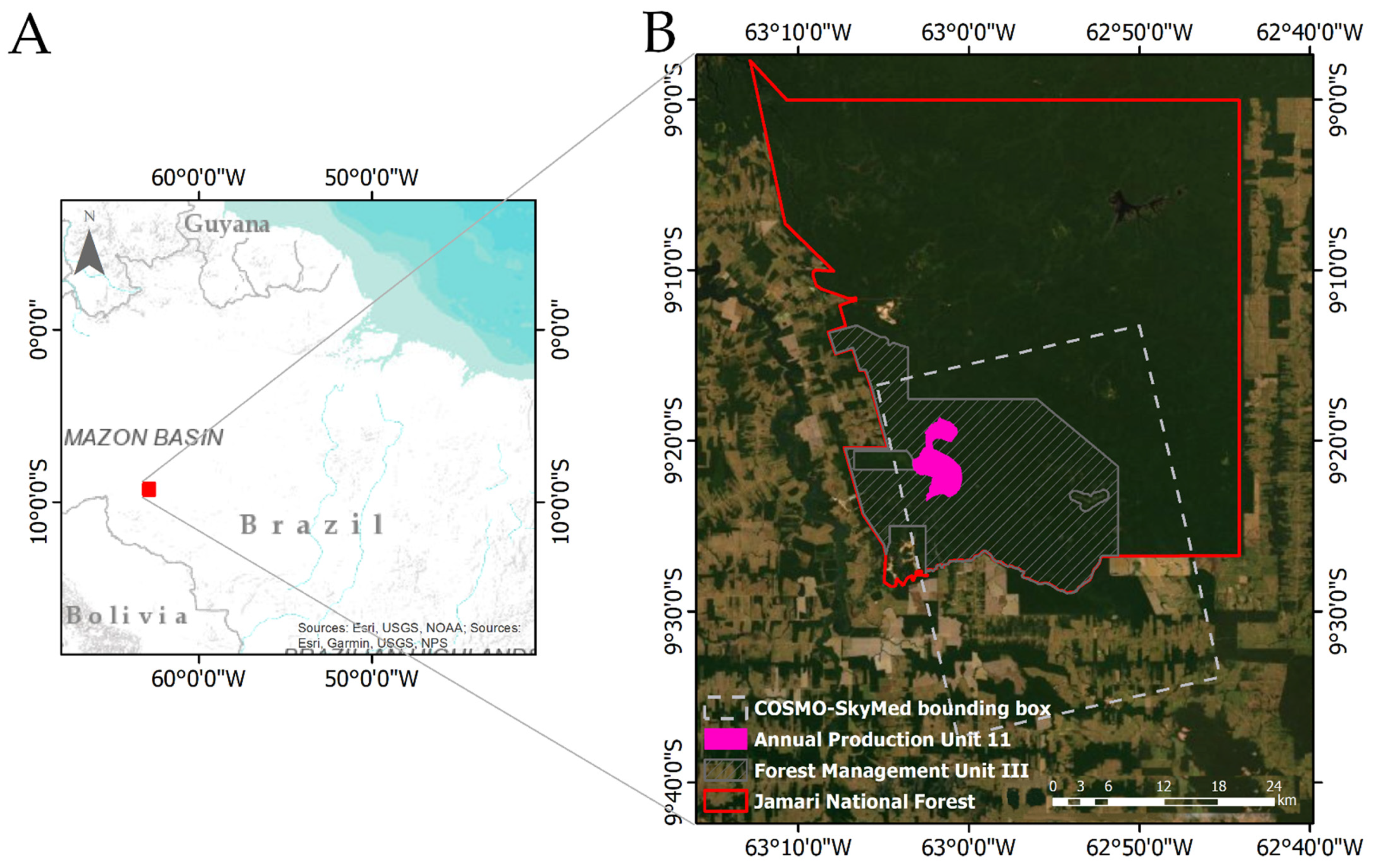
2.1. Study Site and Data

The study area is located in the Jamari National Forest (NF), an area covered by native tropical forest, protected by the Brazilian State. One of the activities allowed in the NFs is sustainable forest management by the concessionaire company that acquired the right to explore the area, which includes selective logging. Jamari NF, which has approximately 220,000 hectares, is subdivided into three Forest Management Units (I, II, and III), which in turn are subdivided into Annual Production Units (UPAs). The UPA explored in 2018 (UPA 11) (Figure 1) was selected for this study because it contains, in addition to the SAR images acquired before and after the exploration period, the forest inventory identifying the exploited trees and the LiDAR point cloud acquired also before and after exploration.

SAR images were acquired on 5 June and 8 October 2018 (before and after the selective logging period) by sensors aboard the COSMO-SkyMed3 and COSMO-SkyMed4 satellites of the COSMO-SkyMed constellation. with the acquisition parameters were wavelength = band X; acquisition mode = STRIPMAP; polarization = HH; angle of incidence = ~55°. The images were processed with 1 look in range and azimuth, resulting in a 3 m grid cell, co-registered for correction of translational and rotational deviations between images, filtered through the GammaMAP filter [45,46] with a 3 × 3 window and, finally, geocoded using the digital elevation model produced from the Phased Array type L-band Synthetic Aperture Radar (PALSAR) sensor and conversion to the backscatter coefficients (σ⁰, units in dB).

The ground truth was generated from airborne LiDAR point clouds acquired in 2018 and 2019 and the forest inventory made available by the Brazilian Forest Service (SFB), the government agency responsible for managing the NFs. The inventory contains the list of tree species that occur in the area, the geographical coordinate of each tree exploited, the date of exploitation, and parameters such as diameter at breast height (DBH), circumference at breast height (CBH), and estimated volume. The LiDAR survey was performed by the LiDAR Optech ALTM Gemini airborne sensor with approximately 21 pulses per square meter of terrain. The data comes from a service contracted by the SFB. Using the LAStools plugin for QGIS [47], these point clouds were converted into a digital surface model (DSM) with 3 × 3 m cells from the first return points, which correspond to the pulses with the shortest time between emission and return, representing those that focused on the outermost surface of the canopy. Given that X-band SAR data interacts only superficially with the canopy and, therefore, understory changes cannot be identified at this wavelength, the purpose of the processing adopted for the LiDAR data aimed to simulate this behavior, which justified the adoption of the first return as a signal to compose the digital model. To identify the selective logging that occurred between the two acquisitions, the ratio between the DSMs was obtained, in which high values represent the changes. The changes were confirmed by overlaying the SAR ratio image with the forest inventory.

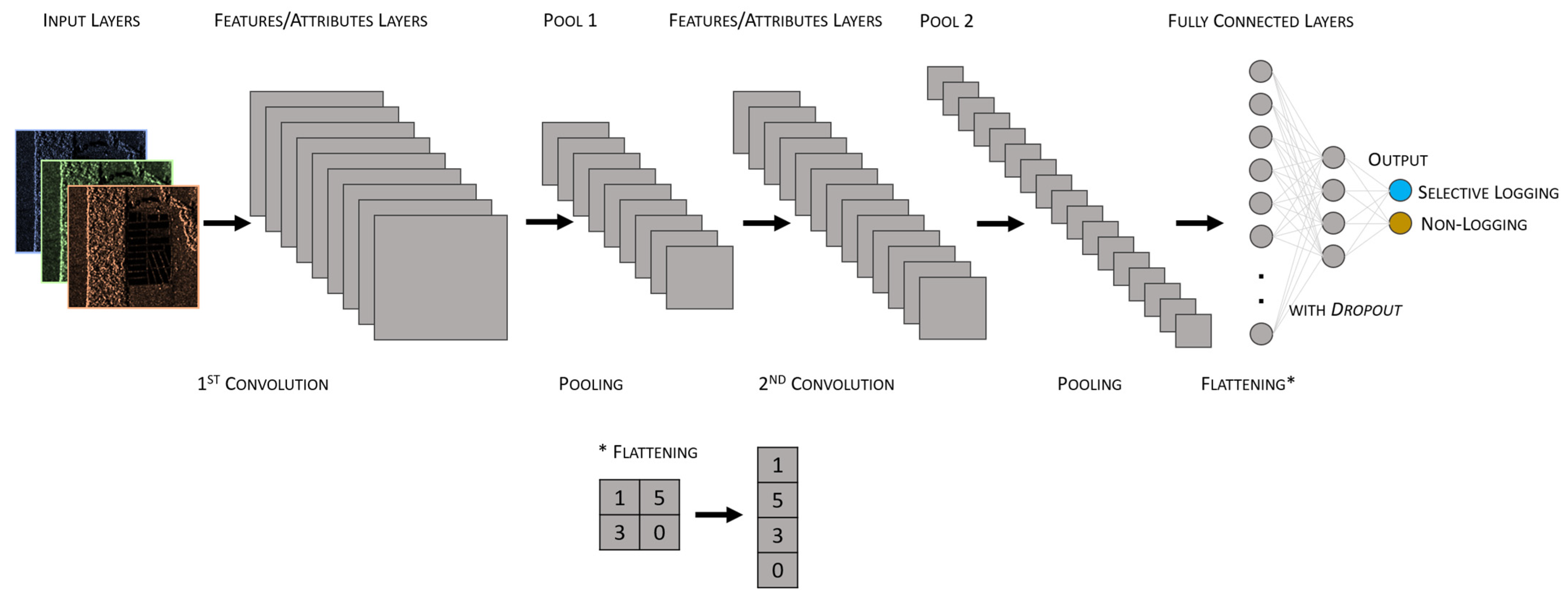
2.2. Convolutional Neural Network Architectures

Convolutional Neural Networks (CNN) are a type of multilayer network with learning capability, composed of convolutional layers, pooling layers, and fully connected layers (Figure 2).

The input of convolutional layers $X\in {ℝ}^{n\times w\times h}$ consists of n 2D feature/attribute maps of size $w\times h$. The output $H\in {ℝ}^{m\times w^{\prime }\times h^{\prime }}$ of the convolutional layers are m 2D feature/attribute maps of size $w^{\prime }\times h^{\prime }$ via convolution matrix W. $W\in {ℝ}^{m\times l\times l\times n}$ are the m trainable filters of size $l\times l\times n$ (usually $l$ = 1, 3, or 5). The convolution process is described as $H=f\left(W\ast X+b\right)$, where * denotes 2-D convolution operation and b the bias. In general, a nonlinear activation function f is performed after the convolution operation. As the convolutional structure deepens, convolutional layers can capture different features/attributes (e.g., edges, lines, corners, structures, and shapes) from the input feature/attribute maps [48].

Pooling layers perform a maximum or average operation over a small area of each input feature map. They can be defined as ${\mathit{H}}_l=pool\left({\mathit{H}}_{l-1}\right)$, where pool represents the pooling function (summarizes the information from that pooling area into a single average, maximum or stochastic pooling value), and ${\mathit{H}}_{l-1}$ e ${\mathit{H}}_l$ the input and output of the pooling layer, respectively. Typically, pooling layers are applied between two successive convolutional layers. The pooling operation can create invariances such as small shifts and distortions. For object detection and image classification, the invariance characteristic provided by pool layers is very important [48].

Fully connected layers usually appear in the upper layer of CNNs, which can summarize the features/attributes extracted from the lower layers. Fully connected layers process their input $\tilde{\mathit{X}}$ with linear transformation by weight $\tilde{\mathit{W}}$ and bias $\tilde{\mathit{b}}$, then map the output of the linear transformation to a nonlinear activation function f, according to the equation $y=f\left(\tilde{\mathit{W}}·\tilde{\mathit{X}}+\tilde{\mathit{b}}\right)$. In the classification task, to generate the probability of each class, a softmax classifier is usually connected to the last fully connected layer. The softmax classifier is used to normalize the output of the fully connected layer $y \in {ℝ}^c$ (where c is the number of classes) between 0 and 1, which can be described as $P\left(y_i\right)=e^{y_i}/{\displaystyle \sum }_{i=1}^c{e}^{y_i}$, where e is the exponential function. The output of the softmax classifier denotes the probability that a given input image belongs to each class. The dropout method [49] operates on fully connected layers to avoid overfitting [49] as a fully connected layer usually contains a large number of parameters [48].

The extraction of attributes from the images occurs through so-called embedders, which read the images and use deep learning models to calculate a vector of attributes for each image. It returns a data table with additional columns containing the image descriptors. The deep learning models tested in this work were:

• InceptionV3 [50]: is Google’s deep neural network for image recognition, consisting of 48 layers. It is trained on the ImageNet dataset [51] and has been shown accuracy greater than 78.1% on this set. The model is composed of symmetric and asymmetric components, including convolutions, average clusters, maximum clusters, concatenations, dropouts, and fully connected layers. Batch normalization is used extensively throughout the model and applied to trigger inputs. The loss is calculated using the softmax function.
• VGG16 [52]: is a convolutional neural network model consisting of 16 layers containing their respective weights, trained in the ImageNet dataset, having achieved 92.6% accuracy in its classification. Instead of having a large number of hyperparameters, the network has convolution layers of 3 × 3 filter with a 1 pass, always using the same padding, and the maxpool layer of 2 × 2 filter with 2 passes. It follows this arrangement of convolution and maxpool layers consistently across the architecture. In the end, there are two fully connected layers, followed by a softmax for the output.
• VGG19: is a variant of the VGG model that contains 19 deep layers, which achieved a 92.7 accuracy in the ImageNet set classification.
• SqueezeNet [53]: is a 26-layer deep convolutional neural network that achieves AlexNet level accuracy [54] on ImageNet with 50× fewer parameters. SqueezeNet employs architectural strategies that reduce the number of parameters, notably with the use of trigger modules that “squeeze” the parameters using 1 × 1 convolutions.
• Painters: is a model trained in the dataset of the Painter by Numbers on Kaggle competition [55], consisting of 79,433 images of paintings by 1584 different painters, whose objective was to examine pairs of paintings, and determine if they are by the same artist. The network comprises a total of 24 layers.
• DeepLoc [56]: is a convolutional network trained on 21,882 individual cell images that have been manually assigned to one of 15 location compartments. It is a prediction algorithm that uses deep neural networks to predict the subcellular location of proteins based on sequence information alone. At its core, the prediction model uses a recurrent neural network that processes the entire protein sequence and an attention mechanism that identifies regions of the protein important for subcellular localization. The network consists of 11 layers.

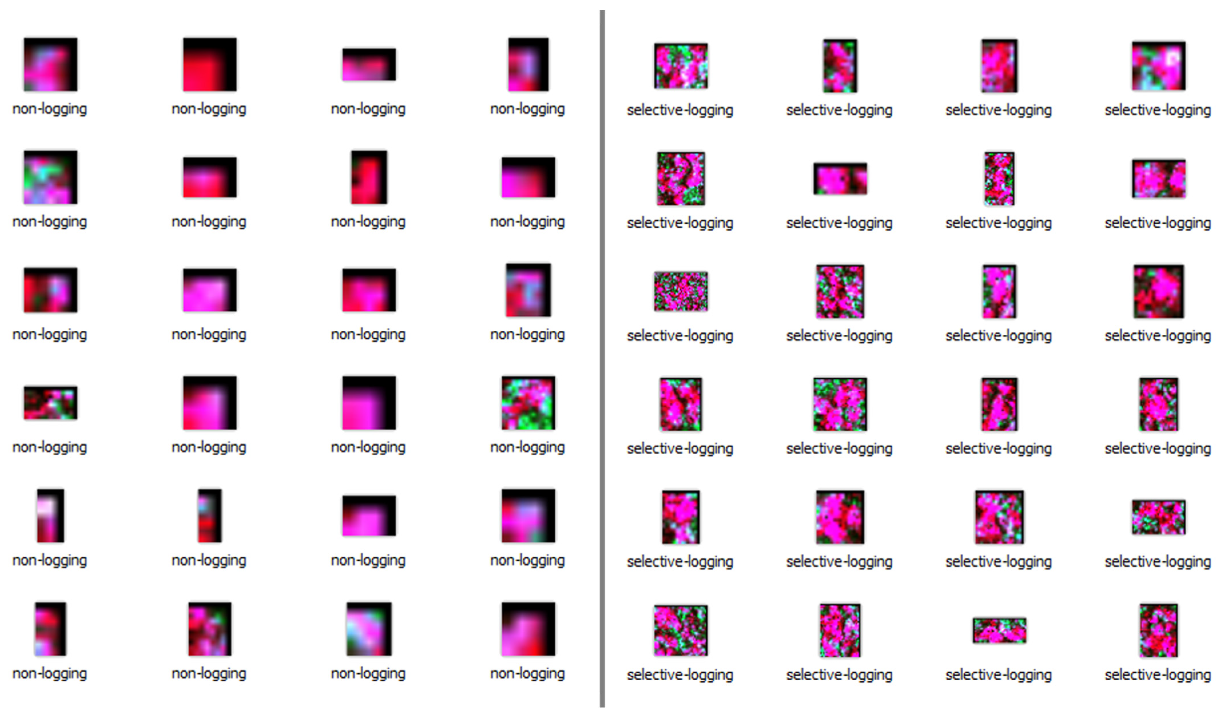
The six models were tested to leverage the transfer learning from their original applications, and thus using the contextual features extracted from their extensive dataset, apply for the forest degradation detection.

2.3. Data Selection

The first stage of the classification tests consisted of selecting all candidate features to change between the SAR images of June/2018 and October/2018. For this, the coefficient of variation (CV) between the two images was generated, since the CV has been pointed out as an advantageous alternative for detecting changes in SAR images [31]. As obtained by [57], the value of 0.4 was defined as the boundary between non-logging and selective logging, thus values greater than 0.4 were included as candidates for the selective logging class. Later, such sets of pixels were vectorized, forming candidate polygons for the selective logging class.

To create a field truth dataset, the extraction class candidates were chosen based on airborne LiDAR and forest inventory data. Thus, of the 186,886 polygons generated by slicing the CV, 4324 received the class label, namely, selective logging and non-logging.

The polygons were then used as a mask to crop the original images listed below into 186,886 patches of varying sizes (depending on feature size—4324 labeled and 182,562 unlabeled, applied for network generalization capacity test and later validated by ground truth), to be used in the CNNs. These models use image patches instead of pixels for training and prediction in order to understand the underlying contextual/textural information.

• RGB whose R channel contains the coefficient of variation image, the G channel the minimum values image and the B channel the gradient (covmingrad image) between the June and October SAR COSMO-SkyMed filtered images;
• RGB whose R channel contains the coefficient of variation image, the G channel the minimum values image and the B channel the gradient (covmingrad image) between the June and October SAR COSMO-SkyMed unfiltered images;
• Single band of the coefficient of variation (CV image);
• Single band of ratio (COSMO-SkyMed_October/COSMO-SkyMed_June—ratio image).

The image clipping procedure generated 4324 labeled sub-images for each of the four images, of which 3026 were used for training and 1298 for testing.

2.4. Classification Tests

The subimages clipped by labeled polygons and classified by field truth were used as training (70%) and test (30%) sets, and the unlabeled ones to analyze the generalizability of CNN. Figure 3 shows a sample of the covmingrad images cut by these polygons.

To perform the tests, the Orange data mining software [58], was adopted, which is a platform for data analysis and visualization based on visual programming that presents the possibility of implementation using the Python 3 library. The general flowchart of the tests is shown in Figure 4.

The tested models were InceptionV3, VGG16, VGG19, SqueezeNet, Painters, and DeepLoc (for details, see Section 2.2). The last fully connected layer was defined according to the tests performed by [57], who presented, as the best result for classification of selective logging, that obtained by an Artificial Neural Network of the Multi Layer Perceptron (ANN-MLP) type, with 1 hidden layer of 50 neurons, with ReLu activation function and SGD weight activator, α = 0.00002 and 1000 iterations (Figure 4, step 5).

The performance evaluation with the test dataset was carried out by calculating the following parameters:

• Area under receiver operator curve (AUC): an AUC of 0.5 suggests no discrimination between classes; 0.7 to 0.8 is considered acceptable; 0.8 to 0.9, excellent; and more than 0.9, exceptional.
• Accuracy: proportion of correctly classified samples.
• Training time (s).
• Test time (s).

The validation strategy adopted was cross-validation [59], with a number of folds = 5. The evaluation of the generalization capacity was carried out based on the accounting, within the area where forest inventory data are available that point the exploited trees, correct classifications, commission and omissions errors, and calculation of the global accuracy [60], that considers data from the diagonal of the confusion matrix (true agreement).

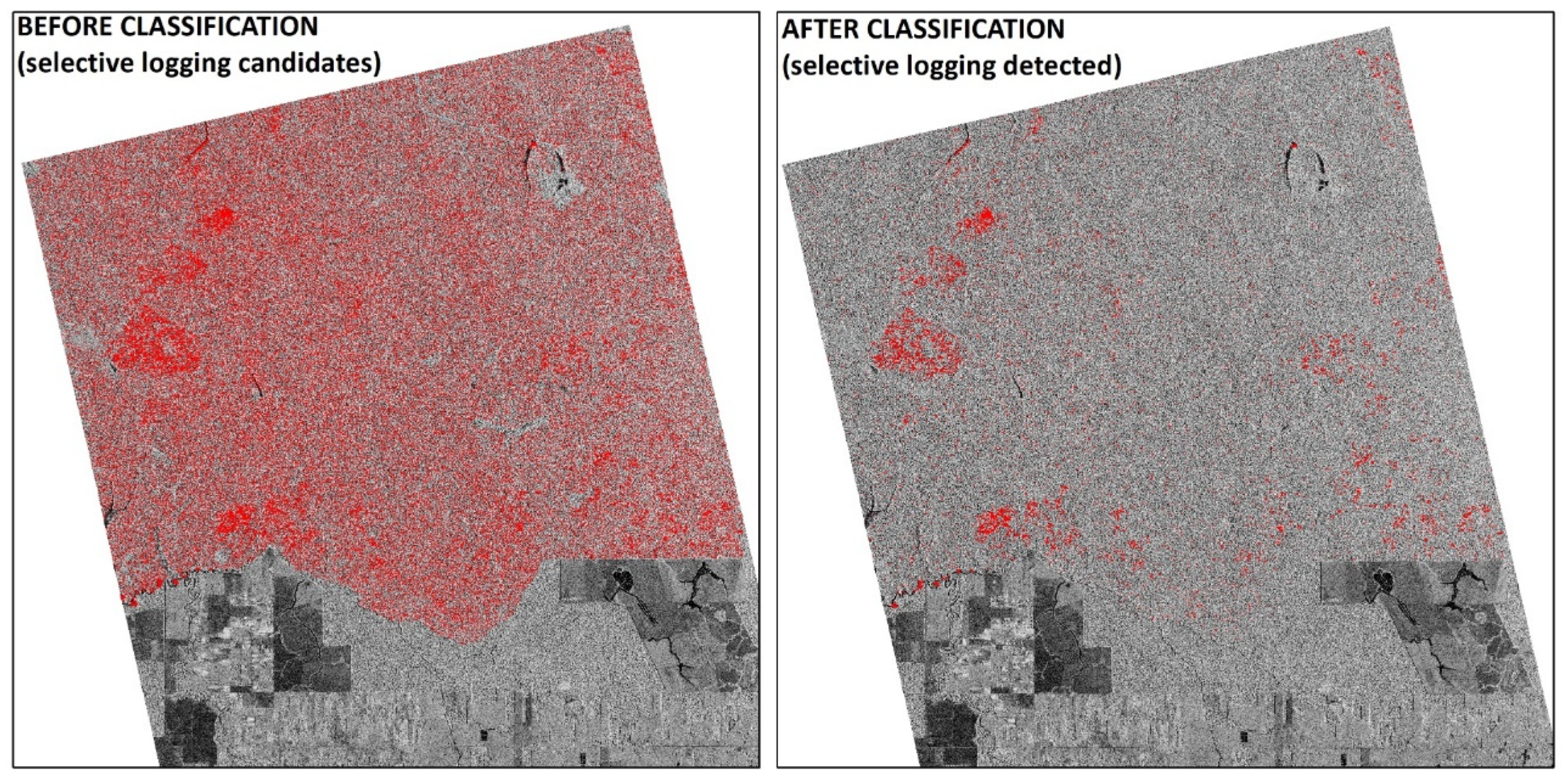
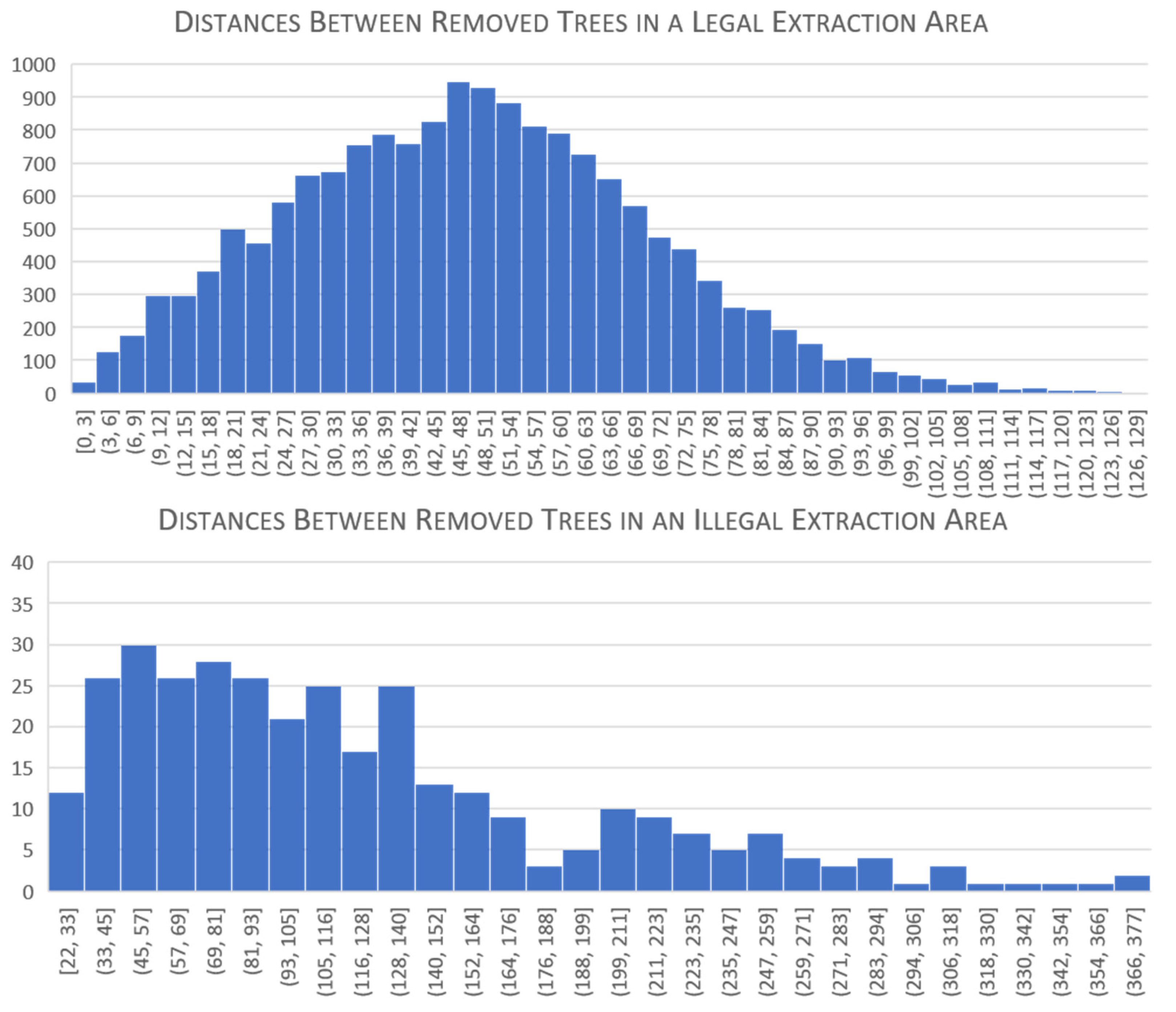
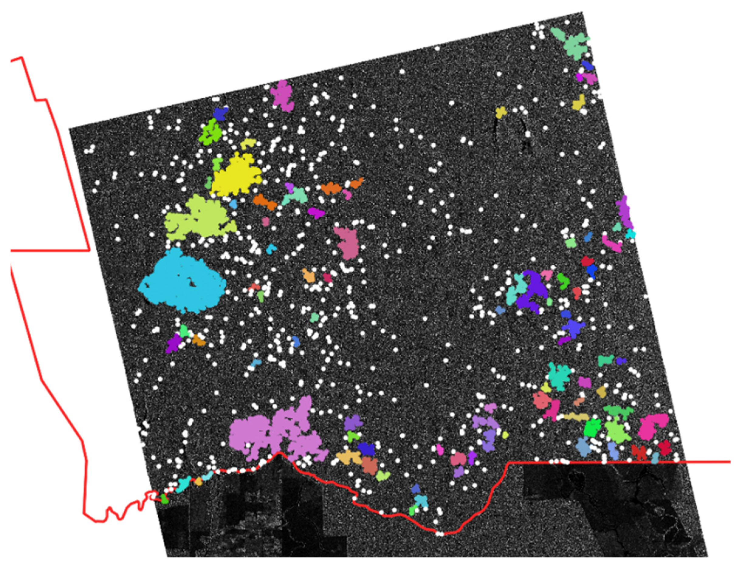
2.5. Grouping of Selective Logging Features

As a final step, a method was proposed that makes it possible to estimate the intensity of exploration (IEX) of the study area, which is calculated by the ratio between the selective logging area (which comprises the area of clearings) and the total area that delimits the region in exploration (minimum bounding box). To delimit the minimum bounding box, the DBSCAN (Density Based Spatial Clustering of Application with Noise) method [61] was applied, which requires two parameters: minimum group size (number of clearings) and maximum distance between grouped clearings, whose definition was based on analysis of the distribution of distances and groupings of available extraction data. The clustering method was performed on polygons classified as selective logging by CNN.

3. Results

The classification tests by pre-trained CNNs on the covmingrad, images are presented in

Table 1. Results of the classification tests by pre-trained CNNs on the covmingrad (A), cov (B), and ratio (C) image. AUC = Area Under the ROC Curve. Numbers in bold represent the best values obtained.

		(A)
Embedder	Train Time (s)	Test Time (s)	AUC	Accuracy
InceptionV3	82.971	1.103	0.953 ± 0.006	0.912 ± 0.009
VGG16	207.532	2.345	0.945 ± 0.009	0.901 ± 0.018
VGG19	385.772	2.547	0.937 ± 0.009	0.907 ± 0.018
SqueezeNet	132.128	0.511	0.954 ± 0.009	0.918 ± 0.018
Painters	124.047	1.064	0.951 ± 0.009	0.920 ± 0.018
DeepLoc	62.666	0.245	0.955 ± 0.009	0.910 ± 0.018
		(B)
Embedder	Train Time (s)	Test Time (s)	AUC	Accuracy
InceptionV3	107.208	1.025	0.948 ± 0.012	0.907 ± 0.026
VGG16	333.649	3.194	0.954 ± 0.009	0.906 ± 0.018
VGG19	239.280	2.851	0.951 ± 0.009	0.899 ± 0.018
SqueezeNet	123.924	0.469	0.943 ± 0.006	0.906 ± 0.009
Painters	105.149	0.807	0.957 ± 0.009	0.911 ± 0.018
DeepLoc	64.436	0.187	0.957 ± 0.009	0.910 ± 0.018
		(C)
Embedder	Train Time (s)	Test Time (s)	AUC	Accuracy
InceptionV3	145.101	1.475	0.838 ± 0.009	0.858 ± 0.018
VGG16	281.361	3.830	0.845 ± 0.002	0.863 ± 0.001
VGG19	285.898	2.321	0.845 ± 0.002	0.860 ± 0.001
SqueezeNet	61.798	0.476	0.850 ± 0.006	0.850 ± 0.009
Painters	125.313	1.031	0.849 ± 0.012	0.858 ± 0.026
DeepLoc	60.500	0.190	0.854 ± 0.009	0.860 ± 0.018

A, on the cov image in Table 1B, and on the ratio image in Table 1C, with all images derived from the filtered COSMO Sky-Med image pair.

The data presented in Table 1A–C shows accuracy values obtained above 85% for all images presented, which are considered excellent results. Considering the confidence intervals calculated between the cross-validation n-folds for a significance level of 5%, there is no significant difference between the accuracies obtained by the models applied to the covmingrad (Table 1A) and cov (Table 1B) images. The models applied to the ratio image, on the other hand, showed lower performance (Table 1C). The best training and testing times were obtained with the DeepLoc embedder for all tests performed. The confusion matrices of the highest mean accuracies obtained through the CNNs tested for each type of input image are presented in Table 1.

Table 2. Confusion matrices of the best accuracy obtained through the CNNs tested for each type of input image.

Covmingrad (Painters)
		Predicted
		selective logging	non-logging
Ground truth	selective logging	85.4%	7.0%
	non-logging	14.6%	93.0%
Cov (Painters)
		Predicted
		selective logging	non-logging
Ground truth	selective logging	83.0%	6.6%
	non-logging	17.0%	93.4%
Ratio (VGG16)
		Predicted
		selective logging	non-logging
Ground truth	selective logging	84.4%	11.2%
	non-logging	15.6%	88.8%

shows that the highest percentage of selective logging correct classifications was obtained with the covmingrad image and Painters model, and therefore, its generalization capacity was tested by applying it to unlabeled images (186,886 images). The confusion matrix containing the results (percentage in relation to the prediction) of the generalization test, obtained by crossing unlabeled images with ground truth, is shown in

Table 3. Confusion matrix containing the results (percentage in relation to the prediction) of the generalization test.

Covmingrad (Painters)—Generalization Test
		Predicted
		selective logging	non-logging
Ground truth	selective logging	87.5%	12.7%
	non-logging	12.5%	87.3%

. The Global Accuracy obtained was 87%. Figure 5 shows the bounding boxes of unlabeled subimages before and after classification.

The highest classification accuracies obtained for unfiltered SAR data (covmingrad images) was the Painters model (89.9%), followed by Inception V3 (89.4%) and SqueezeNet (89.1%) (

Table 4. Results of classification tests by pre-trained CNNs on the covmingrad image from the unfiltered pair of COSMO-SKYMED images. Numbers in bold represent the best values obtained.

Embedder	Train Time (s)	Test Time (s)	AUC	Accuracy
InceptionV3	149.655	1.220	0.931 ± 0.006	0.894 ± 0.009
VGG16	412.935	14.689	0.923 ± 0.009	0.890 ± 0.018
VGG19	496.055	4.399	0.910 ± 0.009	0.871 ± 0.018
SqueezeNet	175.185	0.500	0.923 ± 0.006	0.891 ± 0.009
Painters	169.676	1.239	0.944 ± 0.009	0.899 ± 0.018
DeepLoc	127.549	0.263	0.932 ± 0.009	0.887 ± 0.018

). However, at a significance level of 5%, in this case, it is also not possible to state that there is a significant difference between the results obtained by the different models. The Painters method produced 18.8% commission errors and 8.6% omission errors (

Table 5. Confusion matrix containing the results (percentage in relation to the prediction) of the test with the Painters embedder on the covmingrad image from the unfiltered pair of COSMO-SkyMed images.

Covmingrad (Painters)
		Predicted
		selective logging	non-logging
Ground truth	selective logging	81.2%	8.6%
	non-logging	18.8%	91.4%

).

The Brazilian government, through the Brazilian Forest Service, has developed a system, called DETEX [62], for mapping selective logging. Figure 6 shows the polygons of areas affected by illegal logging in the year 2018. In the same figure, it is possible to observe that detections through CNNs (in magenta) have the advantage of delimiting the scar in the canopy of each tree or set of removed trees, while DETEX (in yellow) presents only a polygon delimiting the affected area.

This precise delimitation of the scar allows, given the correlation between the area of clearings resulting from forest exploitation and the IEX (Exploration Intensity—m³/ha) presented by [63], the estimation of the IEX. In general, the areas of legal exploration, that is, those under concession, have well-defined limits, facilitating the task of estimating the IEX. For illegal exploration areas, an alternative we propose is the grouping of polygons classified as logging, by the DBSCAN (Density Based Spatial Clustering of Application with Noise) method [61], whose required and adopted parameters were the minimum group size (5 gaps) and maximum distance between grouped gaps, defined as 60 m for legal logging and 100 m for illegal logging from the analysis of distances between gaps presented in Figure 7, and calculating the mean values.

Figure 8 shows the grouped gap polygons. The clearings shown in Figure 8 in white color are those that are geographically isolated. For the detection of illegal logging areas, for example, or even for monitoring forest concessions, these clearings could be neglected, as they represent, in many cases, natural tree falls or intense leaf loss. Since logging requires an infrastructure of timber transport, it presents a concentrated pattern of scars rather than a dispersed one. This approach can be especially useful for on-site enforcement efforts, directing operations to areas at an early stage of exploration, reducing the occurrence of false positives.

4. Discussion

Given their low canopy penetrability and relatively low data availability, X-band data are less frequently considered in forestry studies. However, changes in canopy structure caused by vegetation removal can be perceived by sensors operating in high-frequency bands, as they contain more textural information [64], depending on factors, such as biomass, forest structure, and terrain conditions, as they reduce the intensity of backscattered energy, as evidenced by Bouvet et al. [65]. When trees in a forest are extracted, shadows appear or disappear at their edges, depending on the direction of orbit, the position of the fragment in relation to the satellite, and the ground cover around the fragment [65]. The appearance of the shading effect is characterized by the sudden drop in backscatter in a multitemporal series of images acquired according to the same parameters (angle of view, sensor height, orbit, and image acquisition mode). An opposite phenomenon can also be observed in the opposite position of the deforested area: the appearance of an increase in backscattering, which occurs due to the double reflectance effect exerted by the trunks of the remaining trees that are positioned in the direction of propagation of the radar signal [66].

This effect made it possible, as evidenced by Bouvet et al. [65], to detect selective logging occurring in an area of tropical forest in the Brazilian Amazon whose selective logging is authorized by the government. Tests applying pre-trained CNNs on products of the bitemporal pair of COSMO-SkyMed images showed the X-band as suitable for carrying out this type of detection, reaching an accuracy greater than 90% with the use of embedder Painters on covmingrad images. It was able to correctly classify 85.4% of the subimages from the selective logging class and 93% from the non-logging class. Although they did not perform as well, the results of the classification of cov and ratio images presented accuracy above 85%, having correctly classified selective logging s in 83% and 84.4%, respectively.

In general, all models applied to covmingrad and cov filtered and unfiltered images presented good performance, with accuracy above 90%, which proves the ability of these models to classify selective logging in SAR images. These results are similar, in terms of accuracy, to those obtained by [57] with the application of the Artificial Neural Network Multi Layer Perceptron (ANN-MLP) on attributes extracted by the authors of the products of the same bitemporal COSMO-SkyMed images used in this study. The CNNs approach eliminates the attribute generation step, reducing processing time, and its main advantage compared to its predecessors is that it automatically detects and learns texture and context features that describe the target without any human supervision. However, in general, the training time for CNNs was higher than for ANN-MLPs, as CNNs are trained remotely over a large dataset (ImageNet, for example). As the name explains, convolutional networks explore, through multiple filters applied in the convolution windows, textural characteristics of images. Thus, neighborhood relationships between targets (context) are not taken into account, which is an important parameter in the detection of activities such as logging. Kuck et al. [57] explored, in addition to textural parameters, spectral, spatial, and context parameters, and obtained results similar to those of CNNs. A future approach could combine the attributes of the two ML techniques.

The Painters model was selected for the generalizability test, as it showed greater success for the selective extraction class. Embedder Painters was developed within the framework of the Painter by Numbers competition at Kaggle [55], whose objective was to examine pairs of paintings to determine if they were painted by the same artist. The training set consisted of artwork and their corresponding class labels (painters). Its ability to identify the unique styles of painters, in works that do not present standard features, but abstract ones (although characteristic styles and traits, in the case of works by the same painter), may have represented an important characteristic for the classification of selective logging and non-logging, which likewise do not show a shape pattern (unlike the identification of a face, for example, where there is a characteristic pattern).

The classification test of the covmingrad image from unfiltered bitemporal COSMO-SkyMed images resulted in 90% accuracy by the Embedder Painters, being able to correctly classify 81.2% of the selective logging subimages. This result indicates that CNNs are able to correctly classify these targets even under the speckle effect, which, in general, makes it difficult or even impossible to identify targets in SAR images, and its suppression or minimization is the focus of several studies in the microwave remote sensing area [46].

Regarding the grouping methodology presented, in Figure 7 it is possible to see that the distribution is concentrated on the left for the areas of illegal selective logging however, it has a greater variance than the distances presented by the legal selective logging. This is because the legal selective loggings are planned to cause the least possible impact on the forest, and therefore the skid trails are used to transport more than one log, and the trees to be cut are selected according to a plan based on the forest inventory [63]. In illegal logging, this planning and control does not take place. Logging intensity is an important metric given its correlation with damage to the remaining forest. Low understory damage values found are, in part, explained by the low exploration intensity [63].

At the moment, our study is the first one presenting an alternative for operational monitoring of selective logging based on X-band SAR data and CNNs, which allows monitoring even in periods of high cloud cover in the Amazon, which comprises the months between October and April, covering a limitation of optical data [17]. This work demonstrates that such monitoring on a large scale is possible since a well-trained network can have high generalizability. Mitchell et al. [14], in their review of remote sensing applied to the study of forest degradation, presented in 2017 that initiatives using X-band for the purpose of fine-scale detection until that time (logging scars) had no large-scale demonstration or operational application, and in all case studies presented, X-band images were acquired in spotlight mode (VHR covering only a small geographic area) [67]. Having demonstrated high generalizability, it is possible that the technique presented here represents an advance both for operational monitoring and for large-scale application, demanding, however, new tests. Another advance of the study presented is the possibility of detection at the individual level. Although Bullock et al. [15] have obtained high accuracy in detecting degradation through Landsat (optical) images, it is noted that detections are restricted to those intense disturbances (spots of degraded areas, caused by fire or logging infrastructure). One of the first tree level estimates of tree loss come obtained 64% accuracy with a Random Forest model and multi-temporal VHR imagery from WorldView-2 and GeoEye-1 satellites [16]. However, this low accuracy was attributed to view-illumination geometry issues that create shadows not associated with treefalls and tree loss which are inherent in optical data and confuse the classifier. Meanwhile, our estimates and SAR data, in general, do not suffer from these issues, enabling more precise detection of tree loss associated with logging.

Multitemporal SAR data, if acquired under the same geometric and radiometric parameters, present changes related to land cover changes or the presence of dense meteorological formations and changes in the moisture content of the targets. These differences affect backscatter and can produce false detections [5]. More studies should be carried out to quantify the effect of these artifacts on detections through CNNs, although [57] have shown that ANN-MLPs are capable of separating these artifacts from selective logging.

Although we achieved such high accuracy on our method, there are still caveats to be acknowledged. The method confused selective logging with non-logging probably due to foliar loss, natural death of trees, or canopy geometry (trees hidden in the shadow of the neighborhood). This hypothesis must be tested through a field survey that specifically addresses these features. Another potential factor that could affect our estimates is the seasonality and moisture content due to rainfall in the forest. In this experiment, we controlled for seasonality, choosing a pair of images both acquired over the dry season. Further, a previous study pointed out that seasonality might not affect degradation detections using machine learning with X-band SAR data [57]. These aforementioned caveats, thus, consist in some of the directions that future studies can build upon and improve the methodology. Third, we only tested the SAR data COSMO-SkyMed, but perhaps other sensors could be tested such as Iceye and Sentinel-1, including other bands such as C and other acquisitions geometry. We expect this method to be continuously improved and perhaps used for operational monitoring given the availability of SAR data for tropical forest areas.

The deep learning model experiments provided in this paper is the first step towards monitoring tropical forest degradation. This is an important topic in face of climate change and deforestation and degradation reductions pledged by the Brazilian government up to 2030 as recently highlighted in the COP26. We believe our approach can be improved and reach the necessary scale for the operational monitoring towards achieving those difficult but important goals. For this purpose, the investment in SAR data and computing resources by the government would off course be required. Nevertheless, this is a step forward towards fighting forest crime and helping mitigate climate change.

5. Conclusions

Bitemporal features generated from the pair of SAR images used in this study, acquired in X-band and HH polarization by the COSMO-SkyMed constellation before and after the period of legal logging in the Jamari NF, in conjunction with the CNN techniques employed, enabled the detection of scars caused by selective logging in both legal and illegal logging areas. The highest success rate for the selective logging class was obtained by the Painters model. However, in relation to accuracy, all models showed similar performance.

The present study represents an evolution of the study presented by [57], with the advantage that the convolutional network itself extracts the images attributes, eliminating the need for this step in the classification process. The reduction of stages is especially important when the objective is the systematic and operational monitoring of the entire Brazilian Amazon territory, which has an area larger than 5 million km². It is suggested that further studies explore machine learning techniques such as U-NET, based on semantic segmentation, and as input the bitemporal images themselves, eliminating the need to generate bitemporal products (coefficient of variation, ratio, minimum values, and gradient, for example). It is also suggested to increase the training samples and carry out tests in different biophysical composition areas to estimate the generalization capacity of these networks in different environments, and to expand the findings of this study and its advances to automate the application to a regional scale.

The tests showed that CNNs were able to present good results, in the case studied, even when applied to bitemporal products from unfiltered images. Many studies have presented alternatives to reduce the speckle effect on SAR images given that such an effect reduces the target detection and classification capacity of these images. It is suggested that future studies be carried out to measure the contribution of this effect in reducing the performance of techniques based on machine learning for the classification of SAR images.

The DBSCAN clustering method was presented as an alternative for identifying areas at an early stage of illegal selective logging, as well as for measuring the intensity of logging in legal and illegal areas. Although already started, more studies should be carried out to establish the correlation between the area of clearings and the intensity of exploration.

References

1. SEEG-Brasil. Sistema de Estimativa de Emissões de Gases de Efeito Estufa. Available online: http://plataforma.seeg.eco.br/total_emission# (accessed on 20 September 2021).
2. Câmara, G.; Valeriano, D.D.M.; Soares, J.V. Metodologia Para o Cálculo da Taxa Anual de Desmatamento Na Amazônia Legal (PRODES Methodology). Available online: http://www.obt.inpe.br/OBT/assuntos/programas/amazonia/prodes/pdfs/metodologia.pdf/@@download/file/metodologia.pdf (accessed on 23 September 2021).
3. Diniz, C.G.; Souza, A.A.D.A.; Santos, D.C.; Dias, M.C.; Da Luz, N.C.; De Moraes, D.R.V.; Maia, J.S.A.; Gomes, A.R.; Narvaes, I.D.S.; Valeriano, D.M.; et al. DETER-B: The New Amazon Near Real-Time Deforestation Detection System. IEEE J. Sel. Top. Appl. Earth Obs. Remote Sens. 2015, 8, 3619–3628. [Google Scholar] [CrossRef]
4. Watanabe, M.; Koyama, C.N.; Hayashi, M.; Nagatani, I.; Shimada, M. Early-Stage Deforestation Detection in the Tropics with L-Band SAR. IEEE J. Sel. Top. Appl. Earth Obs. Remote Sens. 2018, 11, 2127–2133. [Google Scholar] [CrossRef]
5. Doblas, J.; Shimabukuro, Y.; Sant’anna, S.; Carneiro, A.; Aragão, L.; Almeida, C. Optimizing near Real-Time Detection of Deforestation on Tropical Rainforests Using Sentinel-1 Data. Remote Sens. 2020, 12, 3922. [Google Scholar] [CrossRef]
6. Potapov, P.; Hansen, M.C.; Kommareddy, I.; Kommareddy, A.; Turubanova, S.; Pickens, A.; Adusei, B.; Tyukavina, A.; Ying, Q. Landsat Analysis Ready Data for Global Land Cover and Land Cover Change Mapping. Remote Sens. 2020, 12, 426. [Google Scholar] [CrossRef] [Green Version]
7. Fonseca, A.; Amorim, L.; Ribeiro, J.; Ferreira, R.; Monteiro, A.; Santos, B.; Souza, C., Jr.; Veríssimo, A. Boletim Do Desmatamento Da Amazônia Legal (Maio/2021) SAD. Available online: https://imazon.org.br/publicacoes/boletim-do-desmatamento-da-amazonia-legal-maio-2021-sad/ (accessed on 20 September 2021).
8. Deutscher, J.; Perko, R.; Gutjahr, K.; Hirschmugl, M.; Schardt, M. Mapping Tropical Rainforest Canopy Disturbances in 3D by COSMO-SkyMed Spotlight InSAR-Stereo Data to Detect Areas of Forest Degradation. Remote Sens. 2013, 5, 648–663. [Google Scholar] [CrossRef] [Green Version]
9. Bullock, E.L.; Woodcock, C.E.; Souza, C., Jr.; Olofsson, P. Satellite-Based Estimates Reveal Widespread Forest Degradation in the Amazon. Glob. Chang. Biol. 2020, 26, 2956–2969. [Google Scholar] [CrossRef] [PubMed]
10. Matricardi, E.A.T.; Skole, D.L.; Costa, O.B.; Pedlowski, M.A.; Samek, J.H.; Miguel, E.P. Long-Term Forest Degradation Surpasses Deforestation in the Brazilian Amazon. Science 2020, 369, 1378–1382. [Google Scholar] [CrossRef] [PubMed]
11. Qin, Y.; Xiao, X.; Wigneron, J.P.; Ciais, P.; Brandt, M.; Fan, L.; Li, X.; Crowell, S.; Wu, X.; Doughty, R.; et al. Carbon Loss from Forest Degradation Exceeds That from Deforestation in the Brazilian Amazon. Nat. Clim. Chang. 2021, 11, 442–448. [Google Scholar] [CrossRef]
12. Silva Junior, C.H.L.; Carvalho, N.S.; Pessôa, A.C.M.; Reis, J.B.C.; Pontes-Lopes, A.; Doblas, J.; Heinrich, V.; Campanharo, W.; Alencar, A.; Silva, C.; et al. Amazonian Forest Degradation Must Be Incorporated into the COP26 Agenda. Nat. Geosci. 2021, 14, 634–635. [Google Scholar] [CrossRef]
13. Bullock, E.L.; Woodcock, C.E. Carbon Loss and Removal Due to Forest Disturbance and Regeneration in the Amazon. Sci. Total Environ. 2021, 764, 142839. [Google Scholar] [CrossRef]
14. Mitchell, A.L.; Rosenqvist, A.; Mora, B. Current Remote Sensing Approaches to Monitoring Forest Degradation in Support of Countries Measurement, Reporting and Verification (MRV) Systems for REDD+. Carbon Balance Manag. 2017, 12, 1–22. [Google Scholar] [CrossRef] [PubMed] [Green Version]
15. Bullock, E.L.; Woodcock, C.E.; Olofsson, P. Monitoring Tropical Forest Degradation Using Spectral Unmixing and Landsat Time Series Analysis. Remote Sens. Environ. 2020, 238, 110968. [Google Scholar] [CrossRef]
16. Dalagnol, R.; Phillips, O.L.; Gloor, E.; Galvão, L.S.; Wagner, F.H.; Locks, C.J.; Aragão, L.E.O.C. Quantifying Canopy Tree Loss and Gap Recovery in Tropical Forests under Low-Intensity Logging Using VHR Satellite Imagery and Airborne LiDAR. Remote Sens. 2019, 11, 817. [Google Scholar] [CrossRef] [Green Version]
17. Asner, G.P. Cloud Cover in Landsat Observations of the Brazilian Amazon. Int. J. Remote Sens. 2001, 22, 3855–3862. [Google Scholar] [CrossRef]
18. Mermoz, S.; Le Toan, T. Forest Disturbances and Regrowth Assessment Using ALOS PALSAR Data from 2007 to 2010 in Vietnam, Cambodia and Lao PDR. Remote Sens. 2016, 8, 217. [Google Scholar] [CrossRef] [Green Version]
19. Lee, Y.S.; Lee, S.; Baek, W.K.; Jung, H.S.; Park, S.H.; Lee, M.J. Mapping Forest Vertical Structure in Jeju Island from Optical and Radar Satellite Images Using Artificial Neural Network. Remote Sens. 2020, 12, 797. [Google Scholar] [CrossRef] [Green Version]
20. Bispo, P.C.; Santos, J.R.; Valeriano, M.M.; Touzi, R.; Seifert, F.M. Integration of Polarimetric PALSAR Attributes and Local Geomorphometric Variables Derived from SRTM for Forest Biomass Modeling in Central Amazonia. Can. J. Remote. Sens. 2014, 40, 26–42. [Google Scholar] [CrossRef]
21. Bispo, P.C.; Rodríguez-Veiga, P.; Zimbres, B.; de Miranda, S.C.; Giusti Cezare, C.H.; Fleming, S.; Baldacchino, F.; Louis, V.; Rains, D.; Garcia, M.; et al. Woody Aboveground Biomass Mapping of the Brazilian Savanna with a Multi-Sensor and Machine Learning Approach. Remote Sens. 2020, 12, 2685. [Google Scholar] [CrossRef]
22. Santoro, M.; Cartus, O.; Carvalhais, N.; Rozendaal, D.; Avitabilie, V.; Araza, A.; de Bruin, S.; Herold, M.; Quegan, S.; Rodríguez Veiga, P.; et al. The Global Forest Above-Ground Biomass Pool for 2010 Estimated from High-Resolution Satellite Observations. Earth Syst. Sci. Data 2021, 13, 3927–3950. [Google Scholar] [CrossRef]
23. Deutscher, J.; Gutjahr, K.; Perko, R.; Raggam, H.; Hirschmugl, M.; Schardt, M. Humid Tropical Forest Monitoring with Multi-Temporal L-, C- and X-Band SAR Data. In Proceedings of the 2017 9th International Workshop on the Analysis of Multitemporal Remote Sensing Images (MultiTemp), Brugge, Belgium, 27–29 June 2017; Volume 2017, pp. 1–4. [Google Scholar] [CrossRef]
24. Ghosh, S.M.; Behera, M.D. Aboveground Biomass Estimation Using Multi-Sensor Data Synergy and Machine Learning Algorithms in a Dense Tropical Forest. Appl. Geogr. 2018, 96, 29–40. [Google Scholar] [CrossRef]
25. Treuhaft, R.; Lei, Y.; Gonçalves, F.; Keller, M.; dos Santos, J.R.; Neumann, M.; Almeida, A. Tropical-Forest Structure and Biomass Dynamics from TanDEM-X Radar Interferometry. Forests 2017, 8, 277. [Google Scholar] [CrossRef] [Green Version]
26. Treuhaft, R.; Goncalves, F.; Dos Santos, J.R.; Keller, M.; Palace, M.; Madsen, S.N.; Sullivan, F.; Graca, P.M.L.A. Tropical-Forest Biomass Estimation at X-Band from the Spaceborne Tandem-X Interferometer. IEEE Geosci. Remote Sens. Lett. 2015, 12, 239–243. [Google Scholar] [CrossRef] [Green Version]
27. Delgado-Aguilar, M.J.; Fassnacht, F.E.; Peralvo, M.; Gross, C.P.; Schmitt, C.B. Potential of TerraSAR-X and Sentinel 1 Imagery to Map Deforested Areas and Derive Degradation Status in Complex Rain Forests of Ecuador. Int. For. Rev. 2017, 19, 102–118. [Google Scholar] [CrossRef]
28. Abo Gharbia, A.Y.; Amin, M.; Mousa, A.E.; AbouAly, N.; El Banby, G.M.; El-Samie, F.E.A. Registration-Based Change Detection for SAR Images. NRIAG J. Astron. Geophys. 2020, 9, 106–115. [Google Scholar] [CrossRef] [Green Version]
29. Das, A.; Sahi, A.; Nandini, U. SAR Image Segmentation for Land Cover Change Detection. In Proceedings of the Online International Conference on Green Engineering and Technologies (IC-GET), Coimbatore, India, 19 November 2016. [Google Scholar] [CrossRef]
30. Zhuang, H.; Tan, Z.; Deng, K.; Fan, H. It Is a Misunderstanding That Log Ratio Outperforms Ratio in Change Detection of SAR Images. Eur. J. Remote Sens. 2019, 52, 484–492. [Google Scholar] [CrossRef] [Green Version]
31. Koeniguer, E.C.; Nicolas, J.M. Change Detection Based on the Coefficient of Variation in SAR Time-Series of Urban Areas. Remote Sens. 2020, 12, 2089. [Google Scholar] [CrossRef]
32. Shi, W.; Zhang, M.; Zhang, R.; Chen, S.; Zhan, Z. Change Detection Based on Artificial Intelligence: State-of-the-Art and Challenges. Remote Sens. 2020, 12, 1688. [Google Scholar] [CrossRef]
33. Kaplan, A.; Haenlein, M. Siri, Siri, in My Hand: Who’s the Fairest in the Land? On the Interpretations, Illustrations, and Implications of Artificial Intelligence. Bus. Horiz. 2019, 62, 15–25. [Google Scholar] [CrossRef]
34. Maxwell, A.E.; Warner, T.A.; Fang, F. Implementation of Machine-Learning Classification in Remote Sensing: An Applied Review. Int. J. Remote Sens. 2018, 39, 2784–2817. [Google Scholar] [CrossRef] [Green Version]
35. De, S.; Pirrone, D.; Bovolo, F.; Bruzzone, L.; Bhattacharya, A. A Novel Change Detection Framework Based on Deep Learning for the Analysis of Multi-Temporal Polarimetric SAR Images. In International Geoscience and Remote Sensing Symposium (IGARSS); IEEE: New York, NY, USA, 2017; pp. 5193–5196. [Google Scholar] [CrossRef]
36. Chen, H.; Jiao, L.; Liang, M.; Liu, F.; Yang, S.; Hou, B. Fast Unsupervised Deep Fusion Network for Change Detection of Multitemporal SAR Images. Neurocomputing 2019, 332, 56–70. [Google Scholar] [CrossRef]
37. Lei, Y.; Liu, X.; Shi, J.; Lei, C.; Wang, J. Multiscale Superpixel Segmentation with Deep Features for Change Detection. IEEE Access 2019, 7, 36600–36616. [Google Scholar] [CrossRef]
38. Lv, N.; Chen, C.; Qiu, T.; Sangaiah, A.K. Deep Learning and Superpixel Feature Extraction Based on Contractive Autoencoder for Change Detection in SAR Images. IEEE Trans. Ind. Inform. 2018, 14, 5530–5538. [Google Scholar] [CrossRef]
39. Planinšič, P.; Gleich, D. Temporal Change Detection in SAR Images Using Log Cumulants and Stacked Autoencoder. IEEE Geosci. Remote Sens. Lett. 2018, 15, 297–301. [Google Scholar] [CrossRef]
40. Dong, H.; Ma, W.; Wu, Y.; Gong, M.; Jiao, L. Local Descriptor Learning for Change Detection in Synthetic Aperture Radar Images via Convolutional Neural Networks. IEEE Access 2019, 7, 15389–15403. [Google Scholar] [CrossRef]
41. Li, Y.; Peng, C.; Chen, Y.; Jiao, L.; Zhou, L.; Shang, R. A Deep Learning Method for Change Detection in Synthetic Aperture Radar Images. IEEE Trans. Geosci. Remote Sens. 2019, 57, 5751–5763. [Google Scholar] [CrossRef]
42. Cui, B.; Zhang, Y.; Yan, L.; Wei, J.; Wu, H. An Unsupervised SAR Change Detection Method Based on Stochastic Subspace Ensemble Learning. Remote Sens. 2019, 11, 1314. [Google Scholar] [CrossRef] [Green Version]
43. Jaturapitpornchai, R.; Matsuoka, M.; Kanemoto, N.; Kuzuoka, S.; Ito, R.; Nakamura, R. Newly Built Construction Detection in SAR Images Using Deep Learning. Remote Sens. 2019, 11, 1444. [Google Scholar] [CrossRef] [Green Version]
44. Yosinski, J.; Clune, J.; Bengio, Y.; Lipson, H. How Transferable Are Features in Deep Neural Networks? Adv. Neural Inf. Process. Syst. 2014, 4, 3320–3328. [Google Scholar]
45. Lopes, A.; Nezry, E.; Touzi, R.; Laur, H. Maximum a Posteriori Speckle Filtering and First Order Texture Models in SAR Images. Dig.-Int. Geosci. Remote Sens. Symp. 1990, 28, 992–1000. [Google Scholar] [CrossRef]
46. Kuck, T.N.; Gomez, L.D.; Sano, E.E.; Bispo, P.d.C.; Honorio, D.D.C. Performance of Speckle Filters for COSMO-SkyMed Images from the Brazilian Amazon. IEEE Geosci. Remote Sens. Lett. 2021, 99, 1–5. [Google Scholar] [CrossRef]
47. QGIS.org. QGIS Geographic Information System. Available online: http://qgis.osgeo.org (accessed on 12 September 2021).
48. Cheng, G.; Xie, X.; Han, J.; Guo, L.; Xia, G.S. Remote Sensing Image Scene Classification Meets Deep Learning: Challenges, Methods, Benchmarks, and Opportunities. IEEE J. Sel. Top. Appl. Earth Obs. Remote Sens. 2020, 13, 3735–3756. [Google Scholar] [CrossRef]
49. Srivastava, N.; Hinton, G.; Krizhevsky, A.; Sutskever, I.; Salakhutdinov, R. Dropout: A Simple Way to Prevent Neural Networks from Overfitting. J. Mach. Learn. Res. 2014, 15, 1929–1958. [Google Scholar] [CrossRef] [Green Version]
50. Szegedy, C.; Vanhoucke, V.; Ioffe, S.; Shlens, J.; Wojna, Z. Rethinking the Inception Architecture for Computer Vision. In Proceedings of the IEEE Computer Society Conference on Computer Vision and Pattern Recognition, Las Vegas, NV, USA, 27–30 June 2016; pp. 1–10. Available online: https://arxiv.org/abs/1512.00567 (accessed on 10 September 2021).
51. Deng, J.; Dong, W.; Socher, R.; Li, L.-J.; Li, K.; Fei-Fei, L. Imagenet: A Large-Scale Hierarchical Image Database. In Proceedings of the IEEE Conference on Computer Vision and Pattern Recognition, Miami, FL, USA, 20–25 June 2009; pp. 248–255. [Google Scholar]
52. Simonyan, K.; Zisserman, A. Very Deep Convolutional Networks for Large-Scale Image Recognition. In Proceedings of the 3rd International Conference on Learning Representations, ICLR 2015—Conference Track Proceedings, San Diego, CA, USA, 7–9 May 2015; Available online: https://arxiv.org/abs/1409.1556 (accessed on 12 September 2021).
53. Iandola, F.N.; Han, S.; Moskewicz, M.W.; Ashraf, K.; Dally, W.J.; Keutzer, K. SqueezeNet: AlexNet-Level Accuracy with 50x Fewer Parameters and <0.5 MB Model Size. ICLR 2016, 1–14. Available online: https://arxiv.org/abs/1602.07360 (accessed on 11 September 2021).
54. Krizhevsky, A.; Sutskever, I.; Hinton, G.E. ImageNet Classification with Deep Convolutional Neural Networks. Commun. ACM 2017, 60, 84–90. [Google Scholar] [CrossRef]
55. Nichol, K. Painter by Numbers—Kaggle. Available online: https://www.kaggle.com/c/painter-by-numbers (accessed on 15 September 2021).
56. Almagro Armenteros, J.J.; Sønderby, C.K.; Sønderby, S.K.; Nielsen, H.; Winther, O. DeepLoc: Prediction of Protein Subcellular Localization Using Deep Learning. Bioinformatics 2017, 33, 3387–3395. [Google Scholar] [CrossRef]
57. Kuck, T.N.; Sano, E.E.; Bispo, P.d.C.; Shiguemori, E.H.; Filho, P.F.F.S.; Matricardi, E.A.T. A Comparative Assessment of Machine-Learning Techniques for Forest Degradation Caused by Selective Logging in an Amazon Region Using Multitemporal X-Band SAR Images. Remote Sens. 2021, 13, 3341. [Google Scholar] [CrossRef]
58. Demšar, J.; Curk, T.; Erjavec, A.; Gorup, Č.; Hočevar, T.; Milutinovič, M.; Možina, M.; Polajnar, M.; Toplak, M.; Starič, A.; et al. Orange: Data Mining Toolbox in Python. J. Mach. Learn. Res. 2013, 14, 2349–2353. [Google Scholar]
59. Stone, M. Cross-Validatory Choice and Assessment of Statistical Predictions. J. R. Stat. Soc. Ser. B 1974, 36, 111–133. [Google Scholar] [CrossRef]
60. Congalton, R.G. A Review of Assessing the Accuracy of Classifications of Remotely Sensed Data. Remote Sens. Environ. 1991, 37, 35–46. [Google Scholar] [CrossRef]
61. Ester, M.; Kriegel, H.-P.; Sander, J.; Xu, X. A Density-Based Algorithm for Discovering Clusters in Large Spatial Databases with Noise. In Proceedings of the KDD-96 Proceedings, Portland, OR, USA, 2–4 August 1996; pp. 226–231. Available online: https://www.aaai.org/Papers/KDD/1996/KDD96-037.pdf (accessed on 23 September 2021). [CrossRef]
62. Serviço Florestal Brasileiro. DETEX. Available online: https://www.florestal.gov.br/monitoramento (accessed on 22 August 2021).
63. Locks, C.J. Aplicações da Tecnologia LiDAR no Monitoramento da Exploração Madeireira em Áreas de Concessão Florestal. M.Sc. Thesis, Universidade de Brasília, Brasília, DF, Brazil, 2017. [Google Scholar]
64. van Der Sanden, J.J. Radar Remote Sensing to Support Tropical Forest Management; Tropenbos-Guyana Programme, Georgetown, Guyana, 1997. Available online: https://edepot.wur.nl/121223 (accessed on 10 September 2021).
65. Bouvet, A.; Mermoz, S.; Ballère, M.; Koleck, T.; Le Toan, T. Use of the SAR Shadowing Effect for Deforestation Detection with Sentinel-1 Time Series. Remote Sens. 2018, 10, 1250. [Google Scholar] [CrossRef] [Green Version]
66. Villard, L.; Borderies, P. Backscattering Border Effects for Forests at C-Band. PIERS Online, 2007; Volume 3. Available online: https://www.piers.org/piersonline/pdf/Vol3No5Page731to735.pdf (accessed on 23 September 2021).
67. Kuntz, S.; Astrium, P. White Paper Status of X-Band SAR Applications in Forestry. In Proceedings of the GEO FCT 3rd Science and Data Summit, Arusha, Tanzania, 6–10 February 2012; pp. 6–10. [Google Scholar]
Figure 1. Location of the study area in the Rondônia State, Brazil (A); the study site in the Jamari NF (B).
Remotesensing 13 04944 g001
Figure 2. Schematic diagram of a generic architecture Convolutional Neural Network.
Remotesensing 13 04944 g002
Figure 3. Selective logging and non-logging covmingrad subimages used for CNN training.
Remotesensing 13 04944 g003
Figure 4. Flowchart showing the steps of the classification test by the Convolutional Neural Networks (CNNs). 1. Import of labeled subimages; 2. Embedding and model application to calculate a feature vector for each image; 3. Selection of columns containing the extracted attributes; 4. Splitting the dataset into training and testing sets; 5. Multilayer Perceptron (MLP) classifier (last fully connected layer); 6. execution of tests on the separate set for this purpose and presentation of the results of the quantitative assessment of the classification; 7. Prediction for each subimage; 8. Generation and presentation of the confusion matrix; 9. Visualization of images by class.
Remotesensing 13 04944 g004
Figure 5. Selective logging candidates before and after classification.
Remotesensing 13 04944 g005
Figure 6. Comparison between selective logging detected by CNN (magenta) and by DETEX (yellow).
Remotesensing 13 04944 g006
Figure 7. Distribution of distances between clearings in legal and illegal selective logging.
Remotesensing 13 04944 g007
Figure 8. Polygons classified as logging (grouped—each color represents a group). In red, the Jamari NF limit.
Remotesensing 13 04944 g008