Article

Mapping Flood Extent and Frequency from Sentinel-1 Imagery during the Extremely Warm Winter of 2020 in Boreal Floodplains and Forests

Department of Marine Systems, School of Science, Tallinn University of Technology, Akadeemia tee 15a, 12618 Tallinn, Estonia
*
Author to whom correspondence should be addressed.
Remote Sens. 2021, 13(23), 4949; https://0-doi-org.brum.beds.ac.uk/10.3390/rs13234949
Submission received: 15 October 2021 / Revised: 1 December 2021 / Accepted: 2 December 2021 / Published: 6 December 2021
(This article belongs to the Topic Water Management in the Era of Climatic Change)

Abstract

:
The current study presents a methodology for water mapping from Sentinel-1 (S1) data and a flood extent analysis of the three largest floodplains in Estonia. The automatic processing scheme of S1 data was set up for the mapping of open-water flooding (OWF) and flooding under vegetation (FUV). The extremely mild winter of 2019/2020 resulted in several large floods at floodplains that were detected from S1 imagery with a maximal OWF extent up to 5000 ha and maximal FUV extent up to 4500 ha. A significant correlation (r2 > 0.6) between the OWF extent and the closest gauge data was obtained for inland riverbank floodplains. The outcome enabled us to define the water level at which the water exceeds the shoreline and flooding starts. However, for a coastal river delta floodplain, a lower correlation (r2 < 0.34) with gauge data was obtained, and the excess of river coastline could not be related to a certain water level. At inland riverbank floodplains, the extent of FUV was three times larger compared to that of OWF. The correlation between the water level and FUV was <0.51, indicating that the river water level at these test sites can be used as a proxy for forest floods. Relating conventional gauge data to S1 time series data contributes to flood risk mitigation.

1. Introduction

Near real-time and statistical information about flooded areas is essential for several public services, i.e., emergency, rescue, recovery, spatial planning, habitat monitoring, and adaption to climate change. Satellite remote sensing can provide timely and operational data as well as statistical spatial information about inundated areas covered with water. Two types of satellite imagery are available for monitoring surface flood dynamics: optical and synthetic aperture radar (SAR). Optical satellite remote sensing can only be applied in cloud-free situations. However, floods often occur during long-lasting periods of precipitation and persistent cloud cover. Therefore, SAR systems are usually a preferred tool for the monitoring of floods from space. A smooth open water surface is characterized by a low SAR backscatter, and this difference in backscatter response generally allows flood mapping [1]. Over the last decade, various methods for deriving the flood extent from SAR data have been proposed [2,3,4,5,6,7,8,9,10,11,12,13,14,15,16,17,18]. Based on summaries by Martinis et al. [18] and Liang and Liu [8], the most commonly applied methodology for flood mapping from a single image is histogram thresholding, which can be used in combination with different image processing approaches. Temporal change detection techniques [19,20] and coherence analysis [21] have also been used for open water mapping. However, temporal change detection approaches require two images and can therefore be limited by the temporal coverage of satellite imagery. To improve flood mapping accuracy, the advantages of ancillary data, such as the DEM (digital elevation model) derived HAND (height above the nearest drainage) index and the catchment derived DIST (distance from drainage) index as well as land use map, have been demonstrated in several studies [17,18,20,22]. Most of the proposed approaches for flood mapping are semi-automatic. A fully automatic methodology that integrates split thresholding and fuzzy logic classification has been proposed and applied by Martinis et al. [18] for the processing of TerraSAR-X, and by Twele et al. [23] for the processing of Sentinel-1 (S1).
Recent studies by Grimaldi et al. [24] and Tsyganskaya et al. [25] have summarized the approaches of flood mapping under the forest canopy. The study by Grimaldi et al. [24] shows that the most commonly applied method for the detection of flooded areas under vegetation is the identification of increased backscatter values compared to other objects. The penetration depth of the SAR signal into vegetation is higher for longer wavelengths, so the use of the L-band has been recommended [26,27,28]. However, several studies [20,29,30] have demonstrated the capabilities of C-band and X-band data in the identification of flooded vegetation, especially in the case of sparse forests and leaf-off conditions. Co-polarized signals (HH or VV) are preferred over cross-polarized signals for mapping water under vegetation. Studies have indicated that the use of HH-polarization leads to more accurate results compared to VV-polarization [31,32]. Moreover, the use of polarimetric decomposition and/or interferometric SAR coherence has been utilized for the mapping of floods under vegetation [33]. However, the availability of full polarimetric data is often limited in terms of spatial extent and temporal coverage.
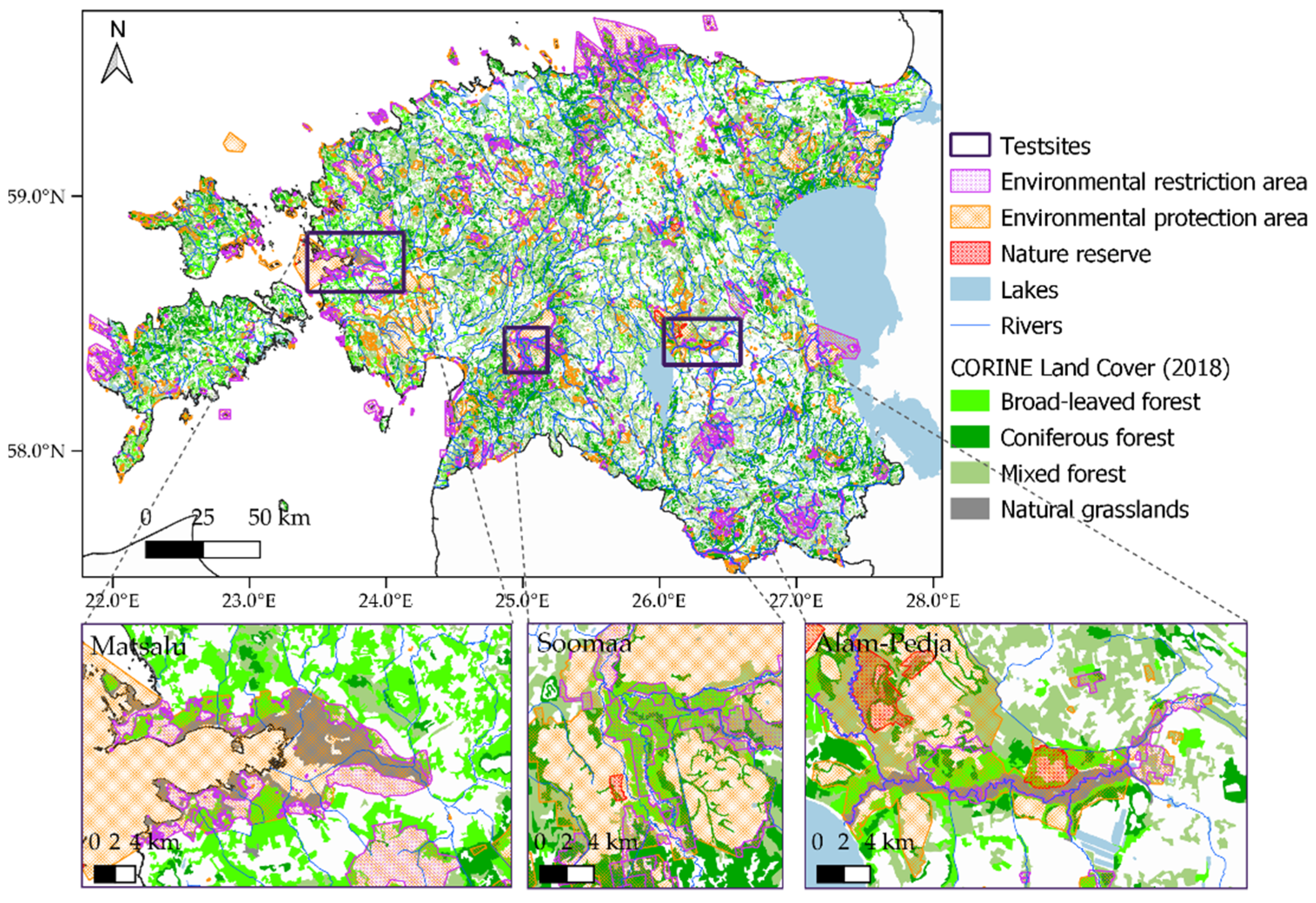
Estonia is known for its large seasonal riverside areas that are flooded over annually. The surface area of the Estonian floodplain grasslands with a high nature conservation value is estimated to be 16,000 hectares. According to the EU Habitats Directive, northern boreal alluvial meadows (habitat type code 6450) are grasslands situated on the banks of large rivers, in sections with slow flow, which are frozen in the winter and flooded in the spring–summer period. However, extremely warm winters in Estonia during the last five years have also caused large flooding during winter [34]. Extreme changes in inundation extent, depth, and duration define phonological patterns, animal migration routes, and human living spaces [35]. Therefore, it is important to monitor the temporal and spatial changes in flooded areas.
The boreal forest encompasses approximately 30% of the global forest area and provides critical services to local, regional, and global populations. Communities benefit from ecosystem services provided by forests for fishing, hunting, leisure activities, and economic opportunities [36]. Countries such as Canada, Finland, Sweden, and Russia extract wood from boreal regions for their forest industries [36]. Flooding causes disturbances in forest management, resulting in economic losses. The vulnerability of the forest ecosystem in a changing climate has been discussed in Gauthier et al. [36] and Hari and Kulmala [37]. Previous studies have expressed the importance of flood monitoring in areas with emerging vegetation for a comprehensive evaluation of the economic and environmental costs of floods [38,39,40]. Recent mild winters in Estonia have affected the forest industry. Forest management is impossible due to unfrozen soils and floods [41]. However, the spatial extent and duration of floods during the winter period in Estonia is still unknown.
At the European scale, two flood-monitoring services are provided. The (1) Copernicus Emergency Management Service (EMS) [42] provides a free-of-charge mapping service in cases of natural disasters, man-made emergencies, and humanitarian crises throughout the world. This service can be triggered by request in the case of an emergency. The (2) Copernicus Land Monitoring Service (CLMS) provides a pan-European, high-resolution product known as Water and Wetness. This product shows the occurrence of water and wet surfaces over the 2009–2018 period. Thematic maps were produced for the years 2015 and 2018. These layers are compiled from multi-temporal high-resolution optical and radar satellite imagery [43].
However, these services do not provide information about the inter-annual variability of water extent on the floodplains, nor information about the flooded forest areas. Therefore, the current study was initiated with the following aims:
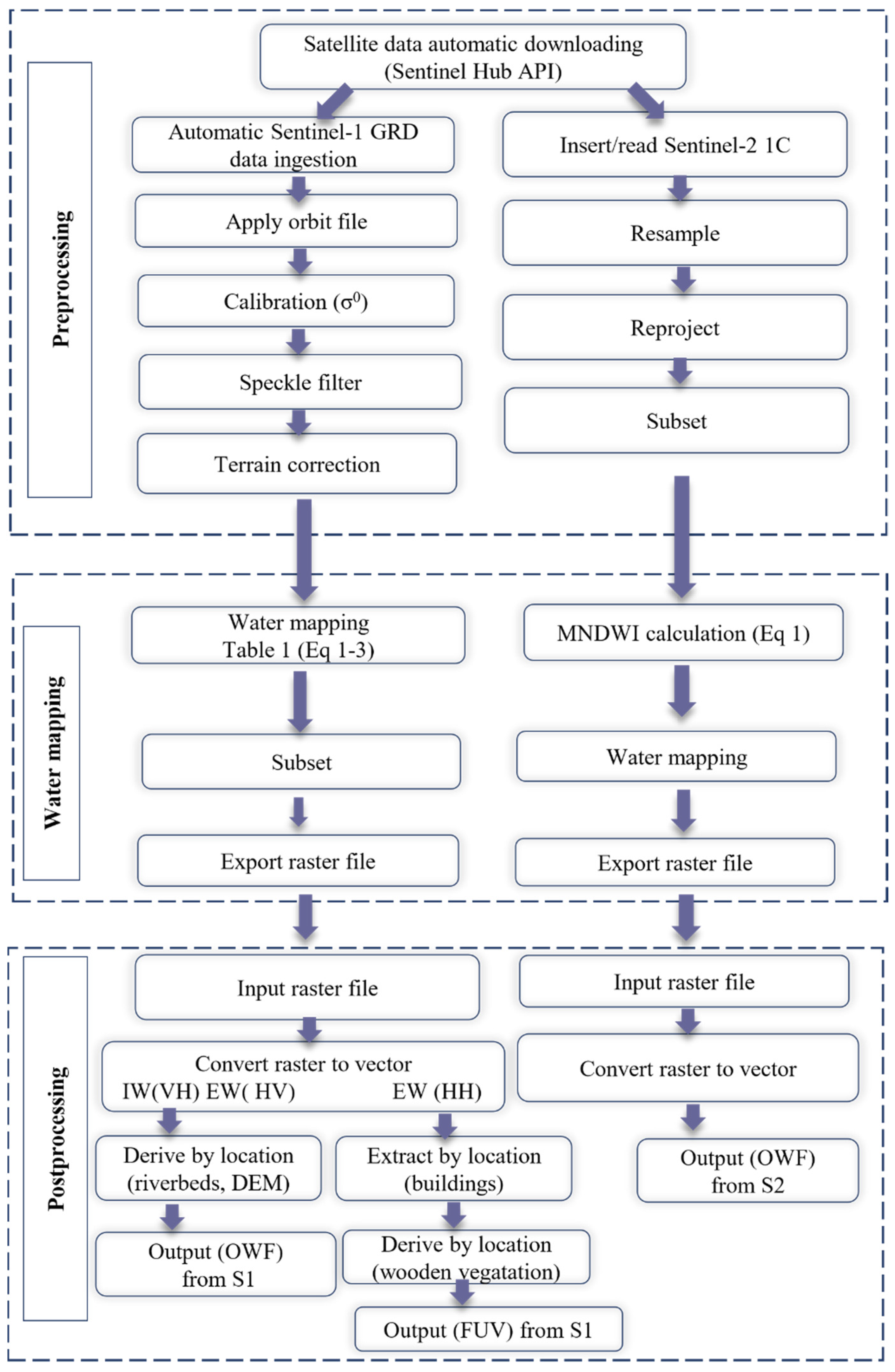
  • Set up an optimal automatic workflow for open-water and flooded forest mapping from S1 data.
  • Apply the workflow for the mapping of flood duration and extent on three of the largest floodplains in Estonia during an extremely mild winter (1 November 2019–31 March 2020).
  • Analyze the correlation between flood extent and the water level measured in the closest hydrological station. Define the water level that indicates the occurrence of flooding (river coastline excess) on floodplains.

2. Study Sites and Data

2.1. Study Sites

Floodplain grasslands can be found all over Estonia, and most of them lie on the larger rivers—Emajõgi, Põltsamaa, Pedja, Kasari, Halliste, Raudna, Piusa, Koiva, Mustjõgi, and Narva headwaters—but some also near lakes (Peipsi, etc.). We chose the three largest floodplain grasslands (Alam-Pedja, Soomaa, and Matsalu) as our study sites. Figure 1 shows study areas with the areas of environmental restrictions, maps of natural grasslands and forests (CLC 2018 from CLMS), and the official shoreline from the Estonian Topographic Database (ETD). Matsalu is a coastal test site located at the River Kasari delta. The defined region of interest used in the analysis of the current study was 1068 km2 (Figure 1). The inland riverbank test sites of Alam-Pedja (located by the River Emajõgi) and Soomaa (located by the Halliste and Navesti rivers) have regions of interest of 546 km2 and 255 km2, respectively (Figure 1, Table 1).
Natural grasslands along rivers have a high nature conservation interest (Figure 1). The habitats of floodplain grassland vegetation are considerably more variable in comparison to boreo-nemoral grasslands—26 different plant communities have been noted as opposed to the 13 found in boreo-nemoral grasslands. Approximately 20–22, maximally 30, bird species are native to the floodplains in Estonia. The share of natural grassland differs between study sites—at Matsalu the share of natural grassland is 7.8% of the study area, while at Soomaa the natural grassland covers 0.8% of the total study area (Table 1).
The share of forest types according to CLC 2018 are shown in Table 1. The dominant forest type at Matsalu and Soomaa is the broad-leaf forest, while at Alam-Pedja the mixed forest type is dominant. The coniferous forest represents the smallest share of forest (Table 1).

2.2. Satellite Data

The S1 mission that carries the C-band SAR sensor provides routine data in two imaging modes: interferometric wide swath mode (IW) and extended wide swath mode (EW). The spatial resolution of the IW mode data is 5 × 20 m, and the spatial resolution of the EW mode data is 20 × 40 m [44]. The Sentinel-2 (S2) optical data are beneficial during cloud-free conditions and have a spatial resolution of 10 × 10, 20 × 20, and 60 × 60 m depending on the wavelength band [45]. The medium spatial resolution data and sufficient repeat cycle of S1 (12 days with one satellite and 6 days with two satellites) and S2 (10 days with one satellite and 5 days with two satellites) missions form a solid basis for statistical flood mapping applications and the operational flood monitoring service [46].
S1 SAR and cloud-free S2 multispectral imager (MSI) data were downloaded from the Copernicus Open Access Hub [47]. The dataset was divided into two parts: (1) algorithm development/validation and (2) algorithm application for statistical analysis. The overview of the data used for algorithm development is given in Table 2. The numbers of images included in the statistical analysis per month at each test site are given in Table 3. To eliminate the water lookalikes caused by thin ice cover, we excluded images that were acquired in the case of negative air temperature from our analysis.

2.3. Auxiliary Data

Auxiliary datasets used in the study include different maps and hydro-meteorological information gathered during the study period.
Maps of wetlands, shorelines, inland waters, wooden areas, and buildings were downloaded from the Estonian Topographic Database (ETD) (provided by the Estonian Land Board) [48]. Maps of areas with environmental restrictions were downloaded from the Estonian Environment Agency WFS service [49]. The digital elevation model (DEM) with a five-meter resolution was downloaded from the Estonian Land Board database [50]. CLC+ (2018) was downloaded from CLMS [43].
Air temperature and water level data measured at national hydro-meteorological stations were obtained from the Estonian Environment Agency [51].
Observations at the time of flooding and UAV flight were performed on 22 March 2019 at the Soomaa test site. In total 44 observations were used for algorithm development.

3. Methodology

3.1. Sentinel-1 Data Processing

We evaluated the sensitivity of S1 polarizations for land and water discrimination [52,53]. The overall backscatter differences resulting from the sensitivity analysis are summarized in Table 4. In the case of the IW imaging mode, the greatest difference between terrestrial and open water signals was obtained for VH polarization (10.5 dB). Data were acquired with an incidence angle of 39.5–47°. In the EW mode, the differences were the greatest for HV polarization (9.6 dB). The data were acquired with an incidence angle of 37.5–46°.
We also evaluated the sensitivity of S1 for the discrimination of flooded forests from dry forest areas. The greatest differences were observed in the case of HH polarization (a difference of 4.5 dB). The data were acquired with an incidence angle of 37.5–46°.
Relying on the sensitivity analysis, the open water mapping algorithm was developed for IW VH and EW HV datasets, and water under vegetation was mapped from EW HH data in the current study.
Previous studies have shown the advantage of using multiple incidence angles for water mapping [54]. Therefore, we established an empirical relationship between the local incidence angle and surface water backscattering collected at our test sites. The dataset of open water backscattering from known waterbodies was collected from 7 IW and 12 EW mode images acquired at the time of flooding in October, November, December, and April in three consecutive years (2017–2019). The relationships between the local incidence angle (θ) and surface water backscattering (σ0) for polarizations with the greatest sensitivity (Table 4 in the previous section) are shown in Figure 2a (original source of data [52]). An established relationship was used for the water mapping algorithm (Table 5) dependency. The algorithms for open water mapping from IW VH and EW HV polarizations are summarized in Table 5.
A study by Lang et al. [55] showed the relationship between the incidence angle and backscatter of water under vegetation. The study demonstrated a decrease in backscatter by 2.45 dB at the incidence angle between 23.5° and 47°, in the case of Radarsat data. For the evaluation of the dependence of incidence angle on the backscattering in the case of a flooded forest, the data were collected at the time of flooding from images acquired on 08 November 2019, 13 November 2019, and 11 April 2018. However, analysis of our dataset did not confirm the relationship between the incidence angle and backscattered signal in a flooded forest (Figure 2b). Relying on our analysis, a threshold condition of HH > −4.21dB was set for flooded forest mapping. The threshold was estimated on an averaged backscattered signal (σ0) +1 standard deviation (SD) in flooded forest areas determined from visual observations.
The data processing scheme was set up in a cluster computing environment. The data processing setup is schematically shown in Figure 3. Pre-processing included the following steps: radar signal calibration, noise filtering, terrain correction, and the image processing technical processes of reading, cutting, and extracting data (Figure 3). Pre-processing was performed using the processors from SNAP (Sentinel Application Platform) software. Water mapping was performed according to Equations (1)–(3) presented in Table 5. The automatic water mapping processes were set up in a cluster computing environment using SHELL script to download the imagery from the Sentinel Open Data Hub and to run SNAP based GPT for water mapping. A combination of the DIST and HAND approaches was applied for the elimination of water lookalikes. The auxiliary data from the Estonian Land Board, namely, the DEM dataset with 5 × 5 m resolution and the official inland water body map (from ETD), were used to improve the mapping accuracy. In the first step of post-processing, the data were polygonised. In the case of inland water bodies, open water polygons (mapped from S1) that intersected with the inland waters map (ETD) with a buffer zone of 100 m were extracted for further analysis. At the coastal zone of the Baltic Sea, the open water polygons that intersected with a coastal area of up to a one meter elevation were extracted for further analysis. GDAL (Geospatial Data Abstraction Library) software processors were used for the post-processing of the data.
In the post-processing of the water mapped under vegetation, the noise (false-positives) from buildings was extracted by removing the polygons that intersected with the buildings map (from ETD). After removal of the areas with elevated backscattering caused by buildings, the water polygons related to the wooden area map (ETD) were extracted for future analysis.

3.2. Sentinel-2 Data Processing

S2 data were used as a validation dataset for an accuracy estimation of the water mapped from S1. S2 data processing is shown in the block scheme in Figure 3. The modified normalized difference water index (MNDWI) was calculated as follows:
MNDWI   = ( Band   3 Band   11 ) / ( Band   3 + Band   11 )
where Band 3 is the top-of-atmosphere (TOA) reflectance of the green band of S2, and Band 11 is the TOA reflectance of the shortwave infrared band of S2. Band 3 and Band 11 have different spatial resolutions of 10 and 20 m, respectively. For the estimation of the MNDWI index, the spatial resolution of Band 11 was scaled to 10 m. In order to determine the water-covered areas from the MNDWI map, the MNDWI > 0.6 condition was applied. The condition was set by visually comparing the Sentinel-2 RGB images to the derived MNDWI map. The relatively high MNDWI threshold is caused by the low values of Band 11 (shortwave infrared) during wintertime. A threshold of 0.6 was sufficient to avoid a large number of false-positive detections.

3.3. Accuracy Evaluation

The accuracy of open-water flood mapping from S1 was evaluated against water mapped from S2 by estimating the overall accuracy and kappa hat coefficient. For accuracy assessment, the Semi-Automatic Classification Plugin in QGIS was used [56]. The kappa hat coefficient (κc) was estimated for the evaluation of classification accuracy between water mapped from S1 and S2 datasets as follows:
κ c = p a p e 1 p e
where pa represents the overall percentage of agreements between S1 and S2 data in raster and pe represents the percentage of chance agreement of S1 and S2 data.
The evaluation of accuracy in the case of water mapped under the vegetation is a complicated task, as water under vegetation cannot be directly mapped from the optical satellite images. The evaluation of water mapped under the vegetation was performed using drone photos and observations (44 observation points) collected at the Soomaa test site on 22 March 2019.

4. Results

4.1. Mapping Accuracy

The open water mapping accuracy from EW HV polarization data was evaluated against the MNDWI index estimated from S2 imagery at three test sites (Table 6, Figure 4). The accuracy of open water mapped from S1 EW HV polarization data at the Matsalu test site was 97.8% with a kappa hat coefficient of 0.94 (Figure 4a, Table 6). The accuracy and kappa hat coefficient of S1 IW VH data from the Alam-Pedja (96.70% and 0.84, respectively; Figure 4c) and Matsalu (95.90% and 0.86, respectively; Figure 4b) test sites were very high, while at the Soomaa test site, the corresponding numbers were lower, 93.60% and 0.62, respectively (Figure 4d).
The evaluation of the water mapped under vegetation was performed using drone photos and observations collected at the Soomaa test site on 22 March 2019. Figure 4e shows the water mapped from S1 images and observation points of the water. As seen in Figure 4e, the validation points coincide with mapped water under vegetation from the S1 EW mode HH data. However, it must be noted that the applied methodology for mapping FUV is less accurate (incidence angle normalization is not applicable) (Figure 2b). Still, we see that statistical analysis enables the identification of areas where water accumulates in forested areas.

4.2. Flood Extent and Frequency for Winter 2019/2020 in Estonian Floodplains

In Figure 5, open water and water under vegetation mapped from S1 data for winter 2019/2020 at our test sites are presented. The winter of 2019/2020 was extremely warm in Estonia. The monthly average temperatures from November 2019 to March 2020 were above zero (Figure 6). Climatological averages for December, January, February, and March have been negative in Estonia in the past (Figure 6). Due to positive air temperatures in the 2019/2020 winter, the soils did not freeze, there was no permanent ice cover on inland waters, and the precipitation was mostly rain. Due to the environmental conditions of winter 2019/2020, open water could be mapped throughout the winter. The flooded area (in hectares—ha) was estimated as the extent of water-covered area outside the official shoreline within the region of interest shown in Figure 1.
At the Alam-Pedja test site, open-water floods occurred near the Emajõgi river. The frequency of flood in pixel varied mainly between 5 and 25%; however, in some areas it reached over 50% (Figure 5a). Figure 5c also shows the water level measured at the Tartu hydrological station on the Emajõgi river and the estimated open-water flood extent. From mid-February, the water covered area repeatedly exceeds the shoreline, and the maximum open-water flood extent (>1000 ha) lasted from February 29 until 15 March 2020 (Figure 5c). In Figure 5, the flood frequency (Figure 5b) and extent (Figure 5d) under the vegetation at the Alam-Pedja test site are also shown. The extent of the flooded area under the vegetation was about three times larger than that of the open-water flood, reaching up to 3500 ha on 13 March 2020 (Figure 5d). However, the frequency of FUV was lower than that of the open-water flood, between 5 and 25%.
At the Soomaa floodplain, the largest flood extent was detected at the beginning of the study period on 7 November 2019, when the open-water flood reached up to 230 ha and the flooded area under the vegetation was 4400 ha (Figure 5g,h). Starting from mid-November, the open-water flood decreased, and the following flood events occurred in mid-December and mid-January. The last flood event lasted from mid-February until mid-March (Figure 5g). The maximal water level measured at the Riisa hydrological station corresponds well to the maximal open-water flood events (Figure 5g). The frequency of open-water flooding remained below 50% in Soomaa. The flood extent analysis revealed that floods detected under the vegetated area lasted through the winter. In the forested area at the Soomaa test site, the floods were absent only during the second half of November (Figure 5h). The flood frequency map presented in Figure 5f indicates the forested areas (dark blue denotes flood frequency >75%) where floods occurred throughout almost the whole duration of the winter.
At the Matsalu test site, large open-water floods outside the official shoreline (ETD) could be detected throughout almost the whole duration of the winter (Figure 5k). The maximum open-water flood extent was detected in March, reaching up to 3000 ha (Figure 5k). In Figure 5i, there is a highlighted area (red rectangle) where open-water floods were observed most frequently (on more than 70% of images). The Matsalu test site has fewer forested areas than the Alam-Pedja and Soomaa test sites. However, there are large areas covered with coastal reed at this test site. The largest floods under the vegetation at this test site are related to an area with coastal reeds (Figure 5j, red rectangle). At the Matsalu test site, the floods under the vegetated area were smaller at 1300 ha (Figure 5k), compared to the open area floods at 3000 ha (Figure 5l).

4.3. Causation Analysis between Flood Extent and Water Level Measured at Hydrological Stations

An analysis was performed with the aim of defining the critical water level at the closest hydrological station that indicates the start of a flooding event (shoreline excess), and to find site specific relationships between the measured water level and flood extent. At the Alam-Pedja test site, a polynomial relationship between the flooded area extent and water level measured at the Tartu hydrological station (HS) was observed (Figure 7). The correlation (r2) with water level was most significant (0.94) for the open-water flood extent estimated from IW VH data; the correlation (r2) for EW HV was 0.85 (Figure 7). The r2 between the flooded area extent under vegetation and the water level measured at the Tartu HS was 0.51 (Figure 7). Our analysis indicated that open-water floodings at the Alam-Pedja floodplain occur when the water level at the Tartu HS increases above 120 cm (Figure 7, red line). Additionally, there was a significant correlation (0.51) between the extent of the flooded area under vegetation and the water level measured at the Tartu HS. It was not possible to define the precise critical water level for the Tartu HS at which flooding under vegetation starts (Figure 7).
The relationship between the water level at the Riisa HS and the flooded area extent at Soomaa was polynomial (Figure 7). The correlation coefficient (r2) between the Soomaa open-water flood extent and the water level measured at the Riisa hydrological station was 0.62 for EW HV data and 0.57 for IW VH data (Figure 7). The correlation (r2) between the water level measured at the Riisa hydrological station and the flooded area extent under vegetation was 0.29 (Figure 7). Our analysis showed that open-water floodings occur when the water level at the Riisa HS increases above 160 cm (Figure 7, red line).
While the relationship between the water level and the extent of the flooded area was polynomial at the Alam-Pedja and Soomaa test sites, the relationship was linear at the Matsalu test site. The r2 between the open-water flood extent at the Matsalu site and the water level measured at the Kasari hydrological station was 0.34 for IW VH data and 0.38 for EW HV data (Figure 7). There was no correlation between the water under vegetation and the water level measured at the Kasari HS (Figure 7). At the Matsalu test site, floods occurred throughout the winter, and it was not possible to define a precise critical water level at the Kasari HS that could be related to the beginning of flooding.

5. Discussion

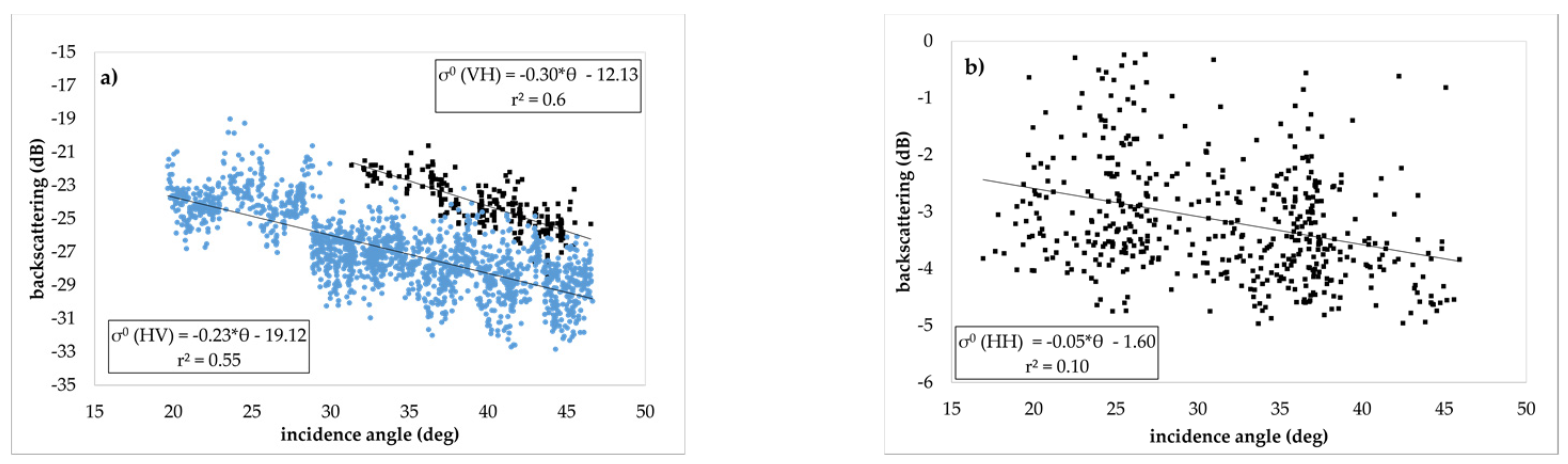
Previous studies have shown the advantages of incidence angle dependent thresholding in the case of TerraSAR-X and Envisat ASAR datasets [18,
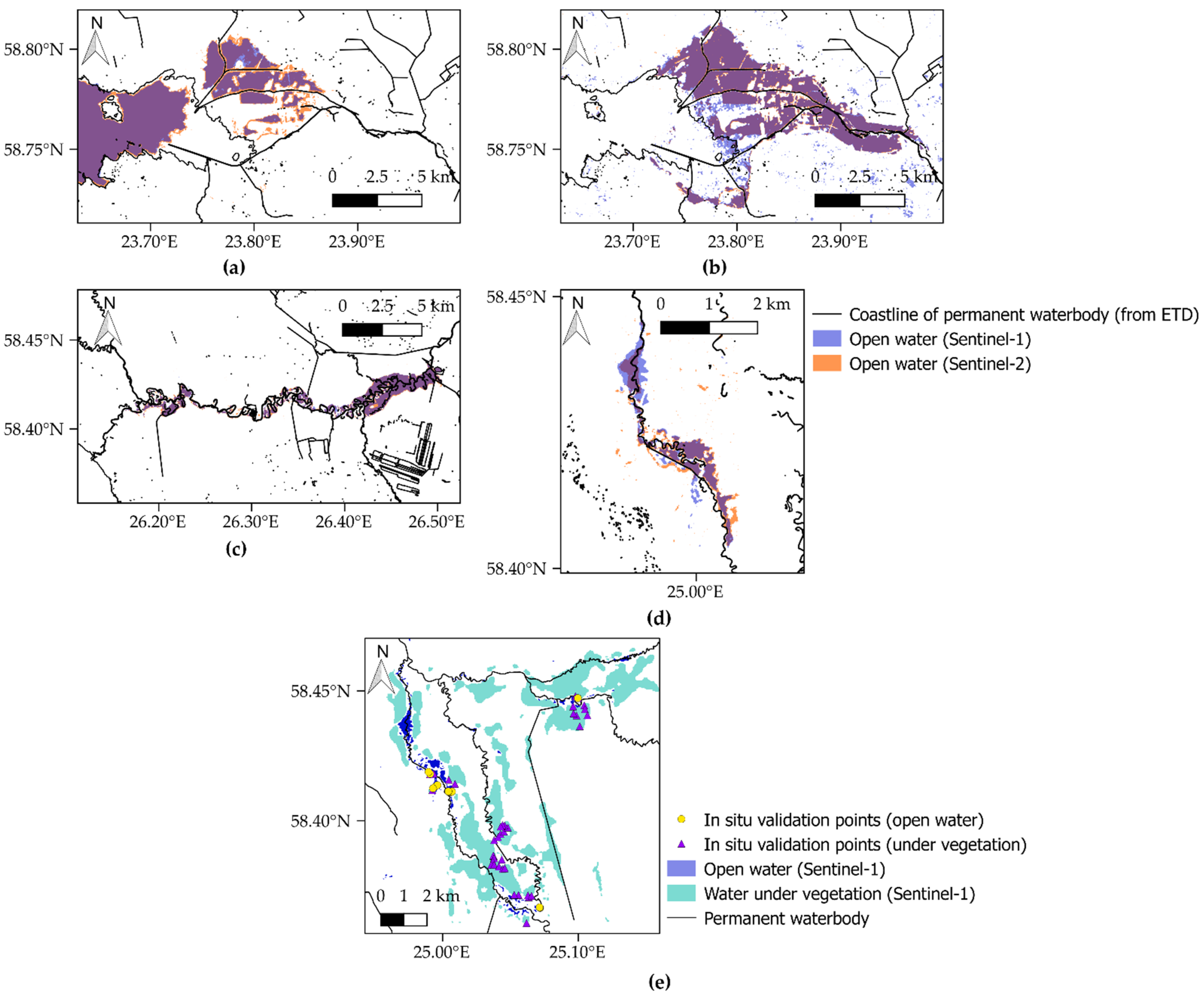
54]. Our operational setup for flood mapping from S1 data for Estonian floodplains integrates incident angle dependent water thresholding and post-processing using auxiliary information from the Estonian Topographic Database. Post-processing using information from the ETD enables the elimination of water lookalikes. We evaluated the open water mapping accuracy for IW mode VH polarization at our test sites. There was good agreement between the water mapped from IW VH data and the S2 MNDWI index, with an accuracy as high as 96.70% and a kappa hat of 0.86 (Table 6). The accuracy of flood mapping using S1 VH polarization has also been evaluated by Twele et al. [23], who obtained a kappa hat coefficient of 0.88 and an accuracy of 94%. While their operational methodology applied for flood mapping differs from that used in our study, the overall accuracy of the flood mapping is comparable. In the study conducted by Twele et al. [23], the split based thresholding for water mapping was used together with the HAND index in the post-processing step.
During the winter season, the default imaging mode of S1 over the Baltic Sea region is the EW regime. To delineate the information about flooded areas in Estonia, an algorithm for open water mapping for the EW regime was established and applied. The open water mapping accuracy from EW HV polarization data was 97.8%. By including the information from EW data, we could delineate the flood maps approximately using 55 images from each test site. Combining the information from IW and EW regimes, we analyzed 83 images from the Alam-Pedja test site, 93 from the Soomaa test site, and 64 from the Matsalu test site for open water mapping for the period of 1 November 2019–31 March 2020 (Figure 5). Thus, the proposed flood mapping method was tested on a large and diverse dataset. The method developed and proposed in the current study has potential for operational mapping of floods in Estonia and neighboring countries (e.g., Latvia).
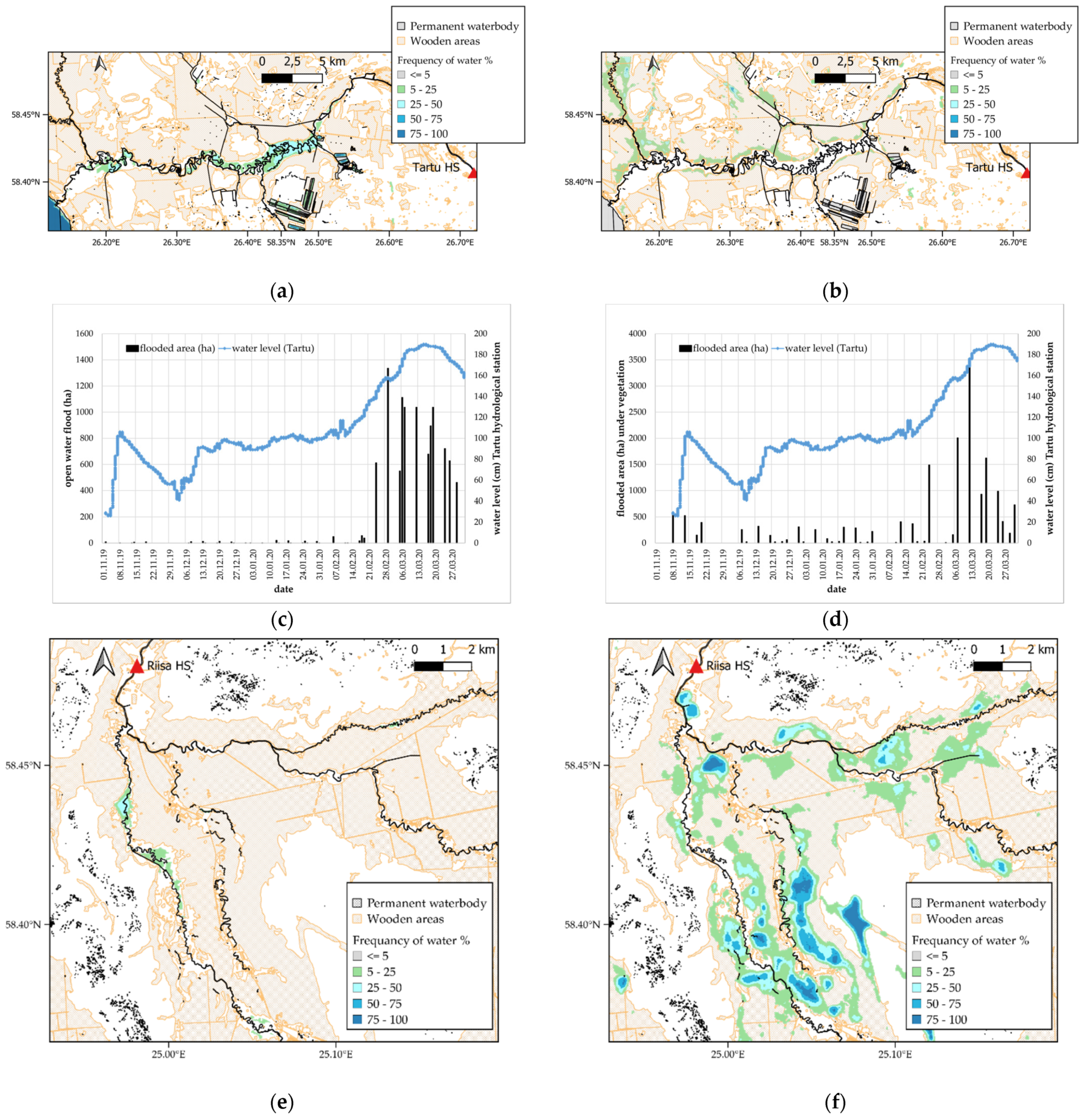
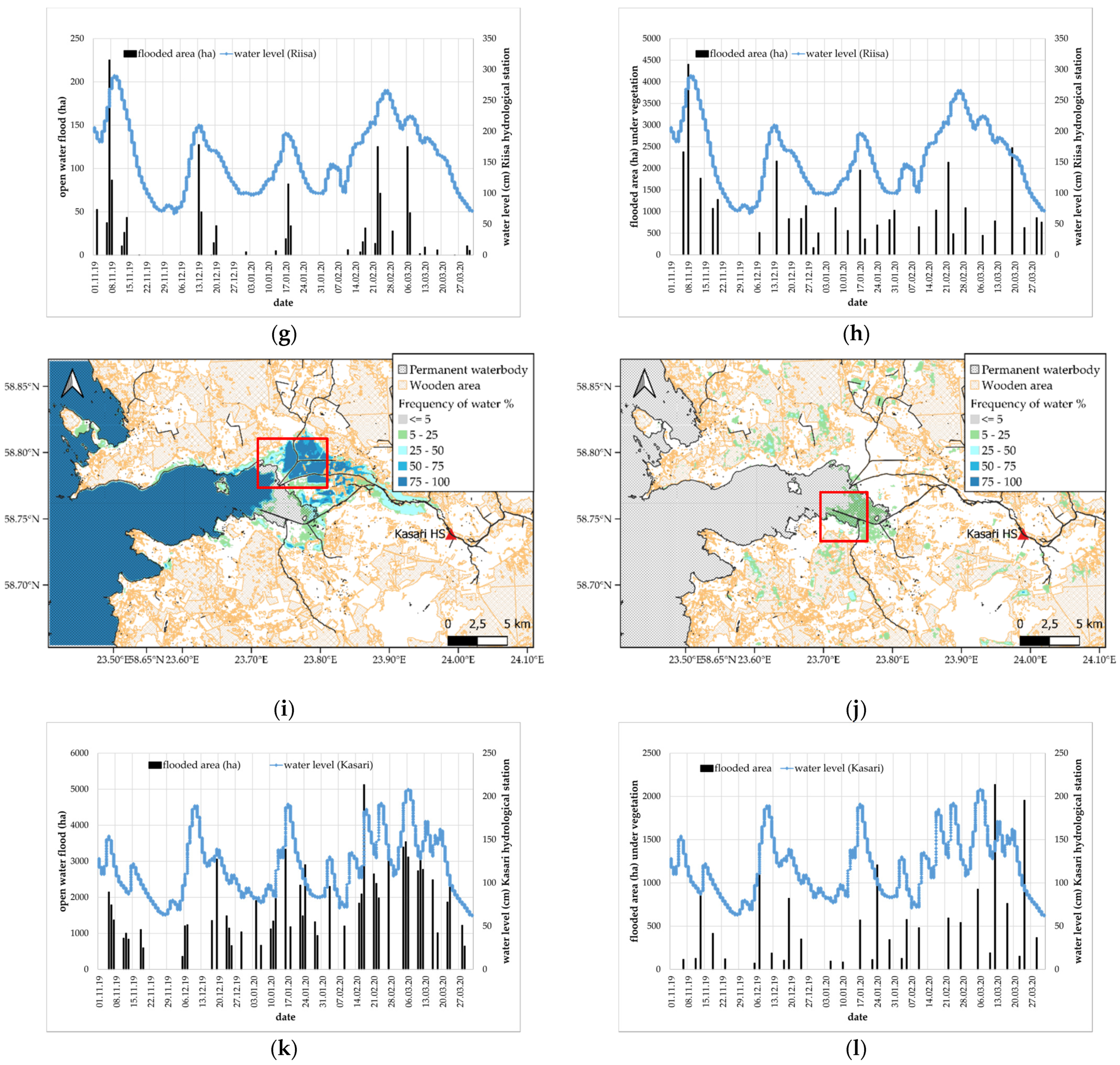
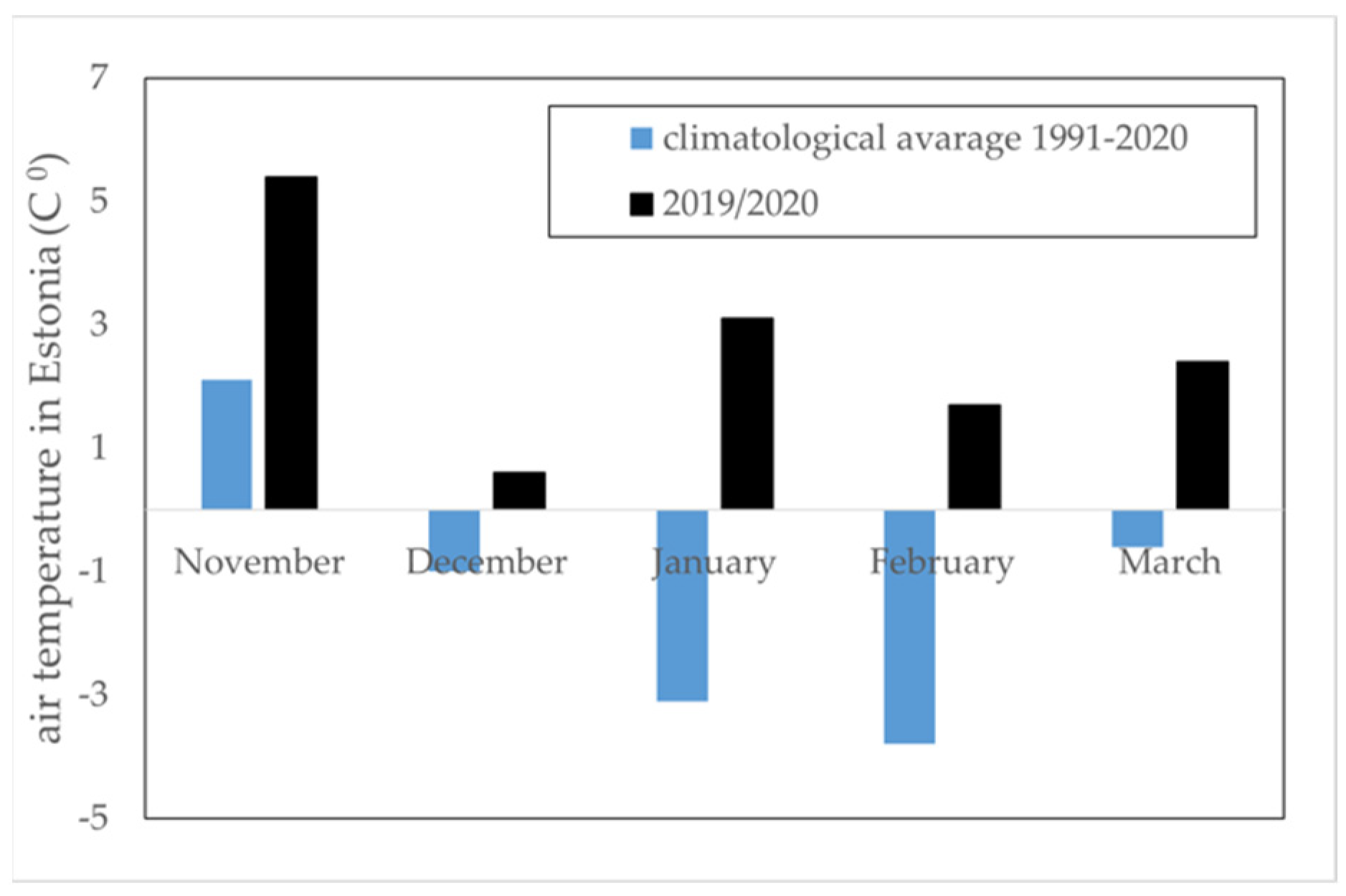
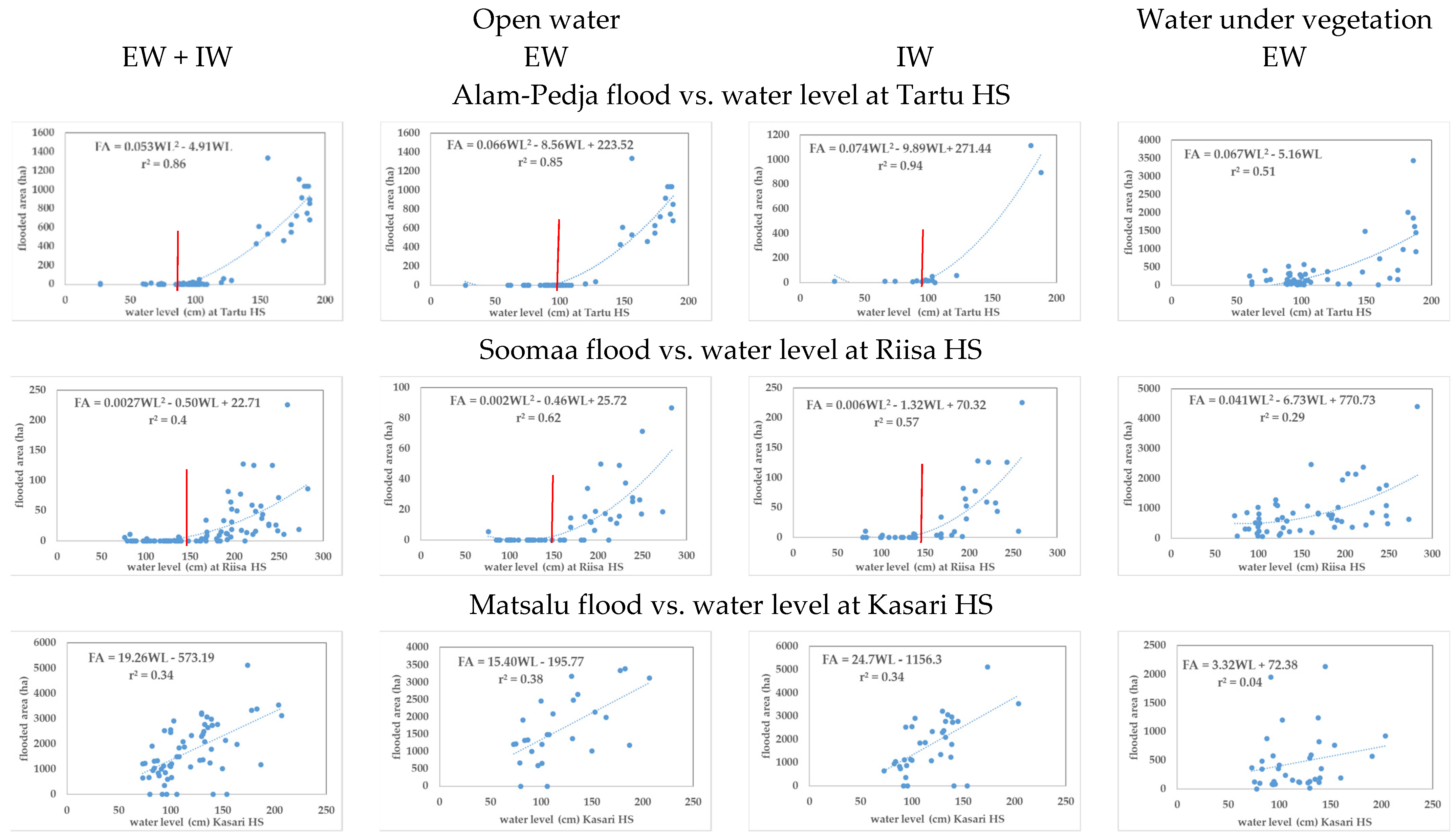
The winter of 2019/2020 was extremely mild in Estonia, and there was no permanent ice on the rivers, nor was there snow cover. The monthly averaged air temperature was above 0 °C at all meteorological stations. Our analysis of flood duration and extent showed that in the winter of 2019/2020, floods were observed almost through the whole period of winter. However, the dynamics of the floods differed between the test sites. The maximum flooding observed at Alam-Pedja occurred in March, while at Soomaa and Matsalu several flood events were detected during the winter of 2019/2020. Analysis of the open-water flood extent and water level measured at the closest hydrological station confirmed the correlation between these variables. The correlation was more significant (r2 < 0.6) for the inland riverside floodplains of Alam-Pedja and Soomaa. For the coastal floodplain at Matsalu, the correlation was 0.34, indicating that the river gauge data cannot be used as proxy for flood extent as the coastal flood was significantly influenced by marine processes (not only by riverine hydrology and precipitation). The analysis also revealed that at Alam-Pedja, floods occur when the water level rises above 120 cm at the Tartu HS. At the Soomaa test site, floods occur when the water level rises above 170 cm at the Riisa HS. At the Matsalu test site, open water outside the official coastline could be observed throughout the winter, and we could not define the precise water level at the Kasari HS that results in a flooding at the floodplain. The Matsalu floodplain is located at the outflow to the Baltic Sea; therefore, it is also influenced by the water level in the sea.
Defining the water level at the closest hydrological station from which the floods start (shoreline excess occurs) can provide information for risk mitigation. Hydraulic modelling is a common tool used in flood risk estimation [57]. However, for hydraulic and hydrological modelling, detailed information about riverbed topography, a digital elevation model of the landscape, and a flow rate are needed. These datasets are not always available; therefore, analysis of remote sensing information in combination with standard gauge data can give valuable information from a single source. S1 time series analysis with local gauge data has been used to determine the positional accuracy of riverside embankments [58]. A study conducted by Wood et al. [58] also pointed out the possibility of determining the positional accuracy of embankments using only a sequence of S1 imagery and gauge data without using topographic data.
In the winter of 2019/2020, several floods in forested areas that harmed economic activities were also reported in the Estonian press [41]. However, the economic loss caused by wintertime flooding in Estonia is unknown. The current study indicated that at the inland riverside floodplains of Soomaa and Alam-Pedja, the flooded areas under vegetation reached up to 4500 ha and were about three times larger than open-water floods at these test sites. Voormasik et al. [30] analyzed the flood extent at Alam-Pedja from TerraSAR-X imagery and estimated the area of flooded forest to be about three times larger than the extent of the open-water flood. Studies indicate that an evaluation of the extent of flooded forest near inland riverbank floodplains is necessary for the estimation of the total flood extent and its economic consequences. Our analysis also revealed that in the case of the inland water floodplains of Alam-Pedja and Soomaa, flood under vegetation could be correlated with the water levels measured at the closest hydrological station.

6. Conclusions

The current paper presents an automatic water mapping method for S1 EW and IW modes by compiling local incident angle thresholding and the application of ancillary information from the Estonian Topographic Database in a post-processing scheme. The proposed method was used to analyze the flood duration and extent in Estonian floodplains during the extremely mild winter of 2019/2020. Our analysis revealed the areas that are most frequently inundated in Estonian floodplains. The observed flood maps allowed us to evaluate the connections between the extent of the flooded area and the water level measured at the closest hydrological station. The study enabled us to determine the water level at which floods occur at the floodplains and to provide valuable information for risk mitigation purposes (standard water level readings from automatic stations are available with a ten-minute interval). The analysis of the extent and frequency of wintertime floods can form the basis for various economic analyses, evaluations of revenue foregone in the forest industry due to mild winters, and evaluations of stress to northern boreal alluvial meadows. The analysis also contributes to the implementation of flood risk assessment and management directive in Estonia [59]. Moreover, the proposed method can be implemented for operational flood mapping in Estonia and neighboring countries.

Author Contributions

Conceptualization, L.S.; methodology, L.S. and A.A.; software, L.S. and A.A.; formal analysis, L.S. and A.A.; writing—original draft preparation, L.S.; writing—review and editing, L.S., A.A. and R.U.; visualization, L.S. All authors have read and agreed to the published version of the manuscript.

Funding

This research was funded by the European Regional Development Fund within the National Programme for Addressing Socio-Economic Challenges through R&D (RITA1/02-52-04) and by Estonian Environment Agency project “Development and implementation of flood monitoring service from satellite remote sensing data” (LLMAE21069).

Institutional Review Board Statement

Not applicable.

Informed Consent Statement

Not Applicable.

Data Availability Statement

The data supporting the conclusions of this article will be made available by the authors, without undue reservation.

Acknowledgments

We would like to thank the Estonian Environment Agency for its cooperation.

Conflicts of Interest

The authors declare no conflict of interest.

References

  1. Ulaby, F.; Moore, R.; Fung, A. Microwave Remote Sensing. Active and Passive; Artech House: Norwood, MA, USA, 1986; Volume 3. [Google Scholar]
  2. Boni, G.; Ferraris, L.; Pulvirenti, L.; Squicciarino, G.; Pierdicca, N.; Candela, L.; Pisani, A.R.; Zoffoli, S.; Onori, R.; Proietti, C.; et al. A Prototype System for Flood Monitoring Based on Flood Forecast Combined with COSMO-SkyMed and Sentinel-1 Data. IEEE J. Sel. Top. Appl. Earth Obs. Remote Sens. 2016, 9, 2794–2805. [Google Scholar] [CrossRef]
  3. Chen, Y.; Fan, R.; Yang, X.; Wang, J.; Latif, A. Extraction of Urban Water Bodies from High-Resolution Remote-Sensing Imagery Using Deep Learning. Water 2018, 10, 585. [Google Scholar] [CrossRef] [Green Version]
  4. Martinis, S.; Twele, A.; Strobl, C.; Kersten, J.; Stein, E. A multi-scale flood monitoring system based on fully automatic MODIS and terraSAR-X processing chains. Remote Sens. 2013, 5, 5598. [Google Scholar] [CrossRef] [Green Version]
  5. Pulvirenti, L.; Pierdicca, N.; Chini, M.; Guerriero, L. An algorithm for operational flood mapping from Synthetic Aperture Radar (SAR) data using fuzzy logic. Nat. Hazards Earth Syst. Sci. 2011, 11, 529–540. [Google Scholar] [CrossRef] [Green Version]
  6. Pulvirenti, L.; Pierdicca, N.; Chini, M.; Guerriero, L. Monitoring flood evolution in vegetated areas using cosmo-skymed data: The tuscany 2009 case study. IEEE J. Sel. Top. Appl. Earth Obs. Remote Sens. 2013, 6, 1807–1816. [Google Scholar] [CrossRef]
  7. Uddin, K.; Matin, M.A.; Meyer, F.J. Operational flood mapping using multi-temporal Sentinel-1 SAR images: A case study from Bangladesh. Remote Sens. 2019, 11, 1581. [Google Scholar] [CrossRef] [Green Version]
  8. Liang, J.; Liu, D. A local thresholding approach to flood water delineation using Sentinel-1 SAR imagery. ISPRS J. Photogramm. Remote Sens. 2020, 159, 53–62. [Google Scholar] [CrossRef]
  9. Schlaffer, S.; Matgen, P.; Hollaus, M.; Wagner, W. Flood detection from multi-temporal SAR data using harmonic analysis and change detection. Int. J. Appl. Earth Obs. Geoinf. 2015, 38, 15–24. [Google Scholar] [CrossRef]
  10. Wendleder, A.; Wessel, B.; Roth, A.; Breunig, M.; Martin, K.; Wagenbrenner, S. TanDEM-X water indication mask: Generation and first evaluation results. IEEE J. Sel. Top. Appl. Earth Obs. Remote Sens. 2013, 6, 171–179. [Google Scholar] [CrossRef] [Green Version]
  11. Chini, M.; Pulvirenti, L.; Pierdicca, N.; Guerriero, L. Multi-temporal segmentation of Cosmo-SkyMed SAR data for flood monitoring. In Proceedings of the 2011 Joint Urban Remote Sensing Event—JURSE 2011, Munich, Germany, 11–13 April 2011. [Google Scholar]
  12. Chini, M.; Hostache, R.; Giustarini, L.; Matgen, P. A hierarchical split-based approach for parametric thresholding of SAR images: Flood inundation as a test case. IEEE Trans. Geosci. Remote Sens. 2017, 55, 6975–6988. [Google Scholar] [CrossRef]
  13. Giustarini, L.; Hostache, R.; Matgen, P.; Schumann, G.J.P.; Bates, P.D.; Mason, D.C. A change detection approach to flood mapping in Urban areas using TerraSAR-X. IEEE Trans. Geosci. Remote Sens. 2013, 51, 2417–2430. [Google Scholar] [CrossRef] [Green Version]
  14. Giustarini, L.; Hostache, R.; Kavetski, D.; Chini, M.; Corato, G.; Schlaffer, S.; Matgen, P. Probabilistic Flood Mapping Using Synthetic Aperture Radar Data. IEEE Trans. Geosci. Remote Sens. 2016, 54, 6958–6969. [Google Scholar] [CrossRef]
  15. Greifeneder, F.; Wagner, W.; Sabel, D.; Naeimi, V. Suitability of SAR imagery for automatic flood mapping in the Lower Mekong Basin. Int. J. Remote Sens. 2014, 35, 2857–2874. [Google Scholar] [CrossRef]
  16. Manjusree, P.; Prasanna Kumar, L.; Bhatt, C.M.; Rao, G.S.; Bhanumurthy, V. Optimization of threshold ranges for rapid flood inundation mapping by evaluating backscatter profiles of high incidence angle SAR images. Int. J. Disaster Risk Sci. 2012, 3, 113–122. [Google Scholar] [CrossRef] [Green Version]
  17. Marti-Cardona, B.; Dolz-Ripolles, J.; Lopez-Martinez, C. Wetland inundation monitoring by the synergistic use of ENVISAT/ASAR imagery and ancilliary spatial data. Remote Sens. Environ. 2013, 139, 171–184. [Google Scholar] [CrossRef]
  18. Martinis, S.; Kersten, J.; Twele, A. A fully automated TerraSAR-X based flood service. ISPRS J. Photogramm. Remote Sens. 2015, 104, 203–212. [Google Scholar] [CrossRef]
  19. Long, S.; Fatoyinbo, T.E.; Policelli, F. Flood extent mapping for Namibia using change detection and thresholding with SAR. Environ. Res. Lett. 2014, 9, 035002. [Google Scholar] [CrossRef]
  20. Clement, M.A.; Kilsby, C.G.; Moore, P. Multi-temporal synthetic aperture radar flood mapping using change detection. J. Flood Risk Manag. 2018, 11, 152–168. [Google Scholar] [CrossRef]
  21. Chini, M.; Pelich, R.; Pulvirenti, L.; Pierdicca, N.; Hostache, R.; Matgen, P. Sentinel-1 InSAR coherence to detect floodwater in urban areas: Houston and hurricane harvey as a test case. Remote Sens. 2019, 11, 107. [Google Scholar] [CrossRef] [Green Version]
  22. Pierdicca, N.; Chini, M.; Pulvirenti, L.; Macina, F. Integrating physical and topographic information into a fuzzy scheme to map flooded area by SAR. Sensors 2008, 8, 4151. [Google Scholar] [CrossRef] [Green Version]
  23. Twele, A.; Cao, W.; Plank, S.; Martinis, S. Sentinel-1-based flood mapping: A fully automated processing chain. Int. J. Remote Sens. 2016, 37, 2990–3004. [Google Scholar] [CrossRef]
  24. Grimaldi, S.; Xu, J.; Li, Y.; Pauwels, V.R.N.; Walker, J.P. Flood mapping under vegetation using single SAR acquisitions. Remote Sens. Environ. 2020, 237, 111582. [Google Scholar] [CrossRef]
  25. Tsyganskaya, V.; Martinis, S.; Marzahn, P. Flood monitoring in vegetated areas using multitemporal Sentinel-1 data: Impact of time series features. Water 2019, 11, 1938. [Google Scholar] [CrossRef] [Green Version]
  26. Henderson, F.M.; Lewis, A.J. Radar detection of wetland ecosystems: A review. Int. J. Remote Sens. 2008, 29, 5809–5835. [Google Scholar] [CrossRef]
  27. Hess, L.L.; Melack, J.M.; Simonett, D.S. Radar detection of flooding beneath the forest canopy: A review. Int. J. Remote Sens. 1990, 11, 1313–1325. [Google Scholar] [CrossRef]
  28. Richards, J.A.; Sun, G.Q.; Simonett, D.S. L-Band Radar Backscatter Modeling of Forest Stands. IEEE Trans. Geosci. Remote Sens. 1987, GE-25, 487–498. [Google Scholar] [CrossRef]
  29. Cohen, J.; Riihimäki, H.; Pulliainen, J.; Lemmetyinen, J.; Heilimo, J. Implications of boreal forest stand characteristics for X-band SAR flood mapping accuracy. Remote Sens. Environ. 2016, 186, 47–63. [Google Scholar] [CrossRef]
  30. Voormansik, K.; Praks, J.; Antropov, O.; Jagomagi, J.; Zalite, K. Flood mapping with terraSAR-X in forested regions in estonia. IEEE J. Sel. Top. Appl. Earth Obs. Remote Sens. 2014, 7, 562–577. [Google Scholar] [CrossRef]
  31. Pierdicca, N.; Pulvirenti, L.; Chini, M.; Guerriero, L.; Candela, L. Observing floods from space: Experience gained from COSMO-SkyMed observations. Acta Astronaut. 2013, 84, 122–133. [Google Scholar] [CrossRef]
  32. Townsend, P.A. Relationships between forest structure and the detection of flood inundation in forested wetlands using C-band SAR. Int. J. Remote Sens. 2002, 23, 443–460. [Google Scholar] [CrossRef]
  33. Brisco, B.; Schmitt, A.; Murnaghan, K.; Kaya, S.; Roth, A. SAR polarimetric change detection for flooded vegetation. Int. J. Digit. Earth 2011, 6, 103–114. [Google Scholar] [CrossRef]
  34. Republic of Estonia, Ministry of the Environment. Climate Change Adaptation Development Plan until 2030; Republic of Estonia, Ministry of the Environment: Tallinn, Estonia, 2017.
  35. Thenkabail, P.S. Remote Sensing Handbook: Remote Sensing of Water Resources, Disasters, and Urban Studies; Taylor & Francis: Boca Raton, FL, USA, 2015; Volume 3, ISBN 9781482217926. [Google Scholar]
  36. Gauthier, S.; Bernier, P.; Kuuluvainen, T.; Shvidenko, A.Z.; Schepaschenko, D.G. Boreal forest health and global change. Science 2015, 349, 819–822. [Google Scholar] [CrossRef]
  37. Hari, P.; Kulmala, L. Boreal Forest and Climate Change; Springer: Dordrecht, The Netherlands, 2008; Volume 34, ISBN 978140208. [Google Scholar]
  38. Dutta, D.; Herath, S.; Musiake, K. A mathematical model for flood loss estimation. J. Hydrol. 2003, 277, 24–49. [Google Scholar] [CrossRef]
  39. Koks, E.E.; Thissen, M.; Alfieri, L.; De Moel, H.; Feyen, L.; Jongman, B.; Aerts, J.C.J.H. The macroeconomic impacts of future river flooding in Europe. Environ. Res. Lett. 2019, 14, 084042. [Google Scholar] [CrossRef]
  40. Molinari, D.; Scorzini, A.R.; Gallazzi, A.; Ballio, F. AGRIDE-c, a conceptual model for the estimation of flood damage to crops: Development and implementation. Nat. Hazards Earth Syst. Sci. Discuss. 2019, 19, 2565–2582. [Google Scholar] [CrossRef] [Green Version]
  41. Estonian Public Broadcasting. Warm Winter Impeding Logging Work. Available online: https://news.err.ee/1021923/warm-winter-impeding-logging-work (accessed on 12 March 2021).
  42. Copernicus Emergency Management Service. Available online: https://emergency.copernicus.eu/mapping/ems/service-overview (accessed on 10 March 2021).
  43. Copernicus Land Monitoring Service. Available online: https://land.copernicus.eu/pan-european/high-resolution-layers/water-wetness (accessed on 10 March 2021).
  44. ESA Sentinel Online. Sentinel-1. Available online: https://sentinel.esa.int/web/sentinel/missions/sentinel-1 (accessed on 12 March 2021).
  45. ESA Sentinel Online. Sentinel-2. Available online: https://sentinel.esa.int/web/sentinel/missions/sentinel-2 (accessed on 12 March 2021).
  46. Zoka, M.; Psomiadis, E.; Dercas, N. The Complementary Use of Optical and SAR Data in Monitoring Flood Events and Their Effects. Proceedings 2018, 2, 644. [Google Scholar] [CrossRef] [Green Version]
  47. Copernicus Open Access Hub. Available online: https://scihub.copernicus.eu/ (accessed on 12 March 2021).
  48. Estonian Land Board. Estonian Topographic Database. Available online: https://geoportaal.maaamet.ee/eng/Spatial-Data/Estonian-Topographic-Database-p305.html (accessed on 12 March 2021).
  49. Estonian Environment Agency. Environmental Restriction Areas. Available online: https://gsavalik.envir.ee/geoserver/eelis/ows? (accessed on 12 March 2021).
  50. Estonian Land Board. Digital Elevation Model. Available online: https://geoportaal.maaamet.ee/est/Ruumiandmed/Korgusandmed/Korgusmudelid-p508.html (accessed on 12 March 2021).
  51. Estonian Environment Agency. Hydrometeorological Data. Available online: http://www.ilmateenistus.ee/teenused/meteoroloogiline-info/ (accessed on 12 March 2021).
  52. Sipelgas, L.; Aavaste, A.; Uiboupin, R.; Rikka, S. Methodology for Mapping Flood Extent on Estonian Floodplains. In Proceedings of the IGARSS 2020—2020 IEEE International Geoscience and Remote Sensing Symposium, Waikoloa, HI, USA, 26 September–2 October 2020; pp. 4750–4753. [Google Scholar]
  53. Sipelgas, L.; Aavaste, A.; Uiboupin, R. Mapping recurrent flooding zone along estonian inland waters from Sentinel-1 and-2. In International Archives of the Photogrammetry, Remote Sensing and Spatial Information Sciences—ISPRS Archives; Copernicus GmbH: Gottingen, Germany, 2020; Volume 43, pp. 627–632. [Google Scholar]
  54. O’Grady, D.; Leblanc, M.; Bass, A. The use of radar satellite data from multiple incidence angles improves surface water mapping. Remote Sens. Environ. 2014, 140, 652–664. [Google Scholar] [CrossRef]
  55. Lang, M.W.; Townsend, P.A.; Kasischke, E.S. Influence of incidence angle on detecting flooded forests using C-HH synthetic aperture radar data. Remote Sens. Environ. 2008, 112, 3898–3907. [Google Scholar] [CrossRef]
  56. Congedo, L. Semi-Automatic Classification Plugin Documentation. 2016. Available online: https://semiautomaticclassificationmanual-v5.readthedocs.io/en/latest/ (accessed on 15 October 2021). [CrossRef]
  57. Brandt, S.A. Modeling and visualizing uncertainties of flood boundary delineation: Algorithm for slope and DEM resolution dependencies of 1D hydraulic models. Stoch. Environ. Res. Risk Assess. 2016, 30, 1677–1690. [Google Scholar] [CrossRef] [Green Version]
  58. Wood, M.; de Jong, S.M.; Straatsma, M.W. Locating flood embankments using SAR time series: A proof of concept. Int. J. Appl. Earth Obs. Geoinf. 2018, 70, 72–83. [Google Scholar] [CrossRef]
  59. European Parliament Council of the European Union. Directive 2007/60/EC of the European Parliament and of the Council of 23 October 2007 on the assessment and management of flood risks. Off. J. Eur. Union 2007, 50, 27–34. [Google Scholar]
Figure 1. Location of the test sites.
Remotesensing 13 04949 g001
Figure 2. (a) Relationship between open-water backscattered signal (σ0) and incidence angle (θ). IW mode data (VH) were acquired from 80 and 58 orbit overflights, and EW mode data (HV) were acquired from 51, 58, 87, 153, and 160 orbit overflights [52]. (b) Relationship between flooded forest backscattered signal (σ0) and incidence angle (θ). EW mode data (HH) were acquired from 51, 58, 87, 153, and 160 orbit overflights.
Remotesensing 13 04949 g002
Figure 3. Data processing setup.
Remotesensing 13 04949 g003
Figure 4. Validation results. (a) Open water mapped from S1 EW HV data vs. S2 MNDWI (4 April 2019), (b) Open water mapped from S1 IW VH data vs. S2 MNDWI (23 March 2019), (c) Open water mapped from S1 IW VH data vs. S2 MNDWI (5 April 2019), (d) Open water mapped from S1 IW VH data vs. S2 MNDWI (16 November 2017) and (e) Comparison of in situ validation points (22 March 2019) with open water mapped from S1 VH data (24 March 2019) and water mapped under vegetation from S1 EW HH data (23 March 2019).
Remotesensing 13 04949 g004
Figure 5. Floods mapped at test sites; (a) Open water frequency (%) at Alam-Pedja, (b) Frequency of water under vegetation (%) at Alam-Pedja, (c) Extent of open-water flood (ha) and water level (cm) at Alam-Pedja, (d) Extent of flood under vegetation (ha) and water level (cm) at Alam-Pedja, (e) Open water frequency (%) at Soomaa, (f) Frequency of water under vegetation (%) at Soomaa, (g) Extent of open-water flood (ha) and water level (cm) at Soomaa, (h) Extent of flood under vegetation (ha) and water level (cm) at Soomaa, (i) Open water frequency (%) at Matsalu, (j) Frequency of water under vegetation (%) at Matsalu, (k) Extent of open-water flood (ha) and water level (cm) at Matsalu, (l) Extent of flood under vegetation (ha) and water level (cm) at Matsalu.
Remotesensing 13 04949 g005aRemotesensing 13 04949 g005b
Figure 6. Meteorological data: monthly average air temperature (black) and corresponding climatological average (blue).
Remotesensing 13 04949 g006
Figure 7. Correlation between flooded area and water level at the closest hydrological station. FA: flooded area extent; WL: water level. Red line denotes the critical water level at which coastline excess occurs and flooding starts.
Remotesensing 13 04949 g007
Table 1. Share of natural grassland and forest types at study sites according to CLC 2018.
Test SiteTotal Size (km2)Broad-Leaved Forest Area (%)Coniferous Forest Area (%)Mixed Forest Area (%)Natural Grasslands Area (%)
Alam-Pedja54611.59.320.95.5
Soomaa10682.04.43.87.8
Matsalu25517.211.111.30.8
Table 2. Numbers of S1 (IW mode and EW mode), S2, and UAV (unmanned aerial vehicle) images used for algorithm development and validation in open water flood (OWF) and flood under vegetation (FUV) conditions.
Purpose of DataS1 IWS1 EWS2UAV
Algorithm development (sensitivity)11
Algorithm development OWF (incidence angle backscattering dependence)712
Algorithm development FUV (incidence angle backscattering dependence) 3
Validation22444
Table 3. Number of images included in analysis per month per test site. OWF represents the number of images from which open-water flood was mapped. FUV represents the number of images from which flood under vegetation was mapped.
Test SiteNov 2019 OWF/FUVDec 2019 OWF/FUVJan 2020 OWF/FUVFeb 2020 OWF/FUVMarch 2020 OWF/FUV
Alam-Pedja13/718/1119/1414/919/13
Soomaa18/1019/1320/1215/921/11
Matsalu10/812/814/610/818/9
Table 4. Summary of sensitivity analysis for land and water discrimination for different S1 polarizations [52].
S1 ModePolarizationWater/Dry Land Difference (dB)Flooded Forest/Unflooded Forest Difference (dB)Range of Incidence Angle
IWVH10.60.1739.5–47
IWVV10.21.3239.5–47
EWHH7.74.537.5–46
EWHV9.60.637.5–46
Table 5. Water mapping threshold conditions for different polarizations, imaging modes, and flood types (FUV and OWF).
S1 ModePolarizationThreshold for Water MappingSDNo
IWVH Water < 0.30 × θ 12.13 + 2 × SD 1.431
EWHV Water < 0.23 × θ 19.12 + 2 × SD 2.262
EWHH Flooded   forest > 3.15 1.06 1.063
Table 6. Validation results. Accuracy and κ c values for different test sites and imaging modes.
LocationDateImaging Mode/PolarizationAccuracy (%) κ c
Matsalu24 September 2019IW/VH95.900.86
Matsalu3–4 April 2019EW/HV97.800.94
Alam-Pedja5 April 2019IW/VH96.700.84
Soomaa16 November 2017IW/VH93.600.62
Publisher’s Note: MDPI stays neutral with regard to jurisdictional claims in published maps and institutional affiliations.

