
Modeling Phenols, Anthocyanins and Color Intensity of Wine Using Pre-Harvest Sentinel-2 Images


1
GeoEnvironmental Cartography and Remote Sensing Group, Universitat Politècnica de València, 46022 València, Spain
2
Hémera Centro de Observación de la Tierra, Escuela de Ingeniería Forestal, Facultad de Ciencias, Universidad Mayor, Huechuraba, Santiago 8580745, Chile
*
Author to whom correspondence should be addressed.
Remote Sens. 2021, 13(23), 4951; https://0-doi-org.brum.beds.ac.uk/10.3390/rs13234951
Submission received: 3 October 2021
/
Revised: 18 November 2021
/
Accepted: 24 November 2021
/
Published: 6 December 2021
(This article belongs to the Special Issue Remote and Proximal Sensing for Precision Agriculture and Viticulture)
Abstract
:The inclusion of technological innovation and the development of remote sensing tools in wine production are an efficient and productive factor that supports the production and improves the quality of the wine produced. In this study we explored models based on Sentinel-2 image bands and spectral indices to estimate key wine quality variables, such as phenols (TP), anthocyanins (TA) and color intensity (CI), providing different sensory characteristics of wine. Two Cabernet Sauvignon wine harvest seasons were studied, 2017 and 2018, and models with coefficients of determination (R2) higher than 60% were obtained for color intensity and total anthocyanins during the first season, both in a period very close to harvest during the first days of April, so the high periodicity of Sentinel 2 becomes strategic. In addition, homogeneous sectors can be identified in the plots for selective harvesting and thus the winery space can be programmed appropriately. These results suggest further work on the number of samples in order to transform it into a useful tool with the potential to define a differentiated harvest and estimate the accumulation of phenolic compounds and the intensity of wine color, key elements in the final quality of the wine.
1. Introduction
In a context of increasing competition in international markets, it has become of utmost importance to achieve higher quality standards in the vineyard. This has led to a renewal of viticulture, a revision of agricultural techniques [1] and the inclusion of technological innovation [2] in the production of wine and in the control of the factors that improve its quality. In red wine, tannins and anthocyanins are the most important phenolic classes. Tannins contribute to the mouthfeel of wines and provide the pigments necessary to give red wine its long-term color stability [3,4]. Anthocyanins are directly responsible for the bluish-red color of red grape skins and naturally for the color of red wine. Phenols are responsible for the color, astringency and bitterness of red wine and contribute to the olfactory profile [5]. Since anthocyanins are located in the skin tissue of most grape cultivars, fermentation and maceration (processes in which the skin is used) have an important effect on the concentration of anthocyanin present in the final wine [6]. In red wines, color is one of the main qualitative parameters. On the one hand, it represents the first organoleptic factor perceived by the taster, and on the other hand, high positive correlations have been determined between color and overall wine quality [7,8]. The main sources of red color in wines come from anthocyanins or their additional derivatives that are extracted or formed during the winemaking process [4,9,10]. Wine color not only provides information about possible defects, the type or state of evolution of the wine, but also has an important influence on acceptability [8]. Even the price of wine is assigned not only by its alcohol content as before, but also by the intensity of its color; therefore, it is of interest to gain knowledge of, to possibly control the factors that affect this parameter [11].
The ripening of the grape (acidity and sugar accumulation) as well as anthocyanin and phenol content and coloring intensity are key variables in the quality of the wine. The degree of total acidity influences the organoleptic characteristics of the wine. In red wines, it influences their coloration, since at a more acidic pH, the anthocyanins that give color to red wine are present in their reddest forms [12]; the pigment of red grapes is affected by the pH of the grapes. Thus, berries with moderate to high acidity will be bright reddish in color and, conversely, berries with low acidity and high pH will tend to be bluish and dark [13].
In this context, developing and using remote sensing tools that allow not only to improve product quality but also to increase efficiency, productivity and input reduction is crucial, as it allows obtaining information quickly, accurately, objectively and non-destructively in almost real time [14].
Recent technological advances have allowed the development of useful tools that help in the monitoring and control of vine growth [1], such is the case of satellite images that provide a synoptic view of the photosynthetically active vine biomass over entire vineyards quickly and cost-effectively. There are several studies that have used Polyphenolic Composition (PC) and Color Intensity (CI) as factors of interest. However, few studies have focused on these factors in produced wine; most have been done in grapes or must, relating NDVI to the berry anthocyanin content [15], tannins [16], Brix and pH [17,18], and pH, polyphenols and color [19]. Some of them especially focused on targeted harvesting and its relationship to various wine quality factors [19,20,21,22,23], as well as on the phenolic content and color in ripe grapes [24]. Other studies were focused on the effects of terroir on berry ripening and composition [25] and on temperatures in relation to anthocyanin and flavonol synthesis [26].
The production of quality wines recognizes that plots are not uniform and therefore require differentiated phytosanitary treatments [27], which would directly benefit grape quality and vineyard profitability [28]. For this reason, it is essential to select the fruit that will be incorporated into the winemaking process [29] based on observable differences in the vigor or vegetative development of the plant or quality parameters of the grape or must [19]. Therefore, identifying intra-parcel variability becomes fundamental during harvest [23], because it improves vineyard yield and grape quality, reducing costs and environmental impact [30,31].
The polyphenolic composition of the wine is conditioned by the quality of the grape and by the vinification method used. Duran and Trujillo (2008) stated that the ripeness of the grapes is of great importance, since the proper development of fermentation depends on the content of sugars and acids and, on the other hand, the color depends on the polyphenolic content, especially anthocyanins and tannins [31]. Considering that (i) various studies have found a relationship between the maturation of the grape and the canopy, and (ii) the polyphenolic composition and color of the wine depends on the maturity of the grape and directly reflect the quality of the wine, we can, therefore, hypothesize that the use of spectral indices derived from satellite images can provide indirect but valuable information regarding the vegetative behavior of the canopy in relation to polyphenolic composition (anthocyanins and phenols) and wine coloring intensity. In addition, knowing its spatial distribution at key moments would help to better plan selective harvesting to produce quality wines. Therefore, acknowledging the importance of anthocyanins, phenols and coloring intensity in the final quality of the wine, this study seeks to define a methodology allowing for the estimation of both the phenolic compounds and color intensity that will be obtained in the final wine, based on spectral information extracted from satellites. Multiple regression analysis between indicators extracted from Sentinel 2 satellite images and data obtained from the winemaking area were used to explore these relationships. The resulting maps of the predicted wine quality parameters could be used as a tool to direct the harvest, contributing to detect intra-parcel variation and to identify zones with homogeneous characteristics of anthocyanins, phenols and coloring intensity.
2. Study Area and Data Collection
This research comprises the study and analysis of data from two wine grape production harvest seasons, 2017 and 2018, from two lots (group of plots) of adult plantations of the Cabernet Sauvignon variety located in Viña Montes winery (Colchagua Valley, VI Region, Chile). The phenological state of the vine until the time of harvest and subsequent vinification was monitored. Micro-vinifications were carried out in order to accurately assess the quality of the wine produced in the samples evaluated.
2.1. Study Area
Within the wine industry, Viña Montes, created in 1987, is a leading company in Chile. In 2011, they implemented a research and development department, which has led them to become a national benchmark. They have a total of 720 hectares of vineyards of which 93% produce wine to export [32,33]. The plantation under study is located in Marchigue, Colchagua Valley in Santa Cruz, VI Region, Chile (Figure 1). This is known as Arcángel and has a total planted area of 499 ha, made up of lots of different varieties such as Cabernet Sauvignon, Syrah and Carmenere, among others, and various quality categories. The area where this study was carried out is made up of 23 plots. A plot corresponds to the polygon that encloses a group of rows of the same vine. In this case, they are grouped into 2 groups or lots: 12 plots formed by 13 polygons, totaling 64.8 ha, and 11 plots formed by 12 polygons, totaling 71 ha, corresponding to plantings in 2007 and 2010 respectively, as shown in Figure 1. The lots are 100% Cabernet Sauvignon, category Alfa, of the intermediate quality category, corresponding to the largest production of Viña Montes, planted according to a 2 × 1 pattern.
In the process carried out at Viña Montes the harvest is mixed, which means this is done manually in lots that are historically identified as of better quality, and mechanized in those of lower quality; however, even this differentiation is not strict and may have some modifications. Therefore, this practice is eventually decided during the course of the harvest process. The lots, or predefined zonings of a lot, are evaluated weekly after veraison (the development period in which grapes change color and begin to ripen), in order to measure the sugar and acid content, two of the most common parameters on which winemakers base their decisions on when to harvest [32]. Such evaluations help to control the grape harvest and winemaking processes and thus meet the demands of winemakers [33]. Defining when and which plots will be harvested is based solely on the organoleptic evaluation that is carried out in the field daily, a task that takes between 10 and 30 min per sampling site. Therefore, only one sample is collected per visit, which is expected to be representative of the entire plot.
2.2. Vine Cycle Climate of the Study Area
Most of the world’s wine production takes place in Mediterranean climates, characterized by high temperatures during the summer, high light intensity and humidity levels that decrease sharply throughout the day [34]. Soil and climate conditions are key for vines, so that the same grape variety, at a similar degree of ripeness but grown in two different areas, may result in two different wines [35,36,37,38]. This is the reason why terroir is important, which we can define as the extension of land whose natural characteristics are a unique set of factors (soil, terrain and climate); therefore, it is the terroir that imprints a distinctive seal onto the wine [35,36]. The study area is dominated by a warm Mediterranean-type temperate climate [38] with a dry season of six months and a rainy winter, with a total annual precipitation between 400 and 600 mm. Additionally, the soils are of alluvial origin, with silt loam textures [39].
The vegetative cycle begins when the buds start growing in early spring (September or October) and generally ends from April to May. The cycle may have some variations that are influenced by differences in temperature and precipitation conditions [40]. An increase in average temperatures and a reduction in thermal oscillation influence varietal aroma and wine color.
The 2017 phenological cycle is marked by the 2016 rainfall, scarce compared to the cumulative rainfall of 2017 (2018 grapevine phenological cycle), which doubled compared to 2016 (Figure 2a). In the 2018 season, the air temperature was relatively lower than in 2017 during the grapevine ripening cycle. The mean temperature difference reached 2 °C, which is equivalent to 11% decrease in that period. Figure 2b shows the comparison of these differences in degrees Celsius with respect to the DOY (day of year).
2.3. Data Collection
The images used were acquired from the Sentinel 2A and Sentinel 2B platforms and downloaded at processing Level-1C, then atmospherically corrected to obtain surface reflectivities, using the Sen2cor application in the SNAP environment (Sen2Cor v2.9 developed by ESA, last access on: http://step.esa.int/main/snap-supported-plugins/sen2cor/sen2cor-v2-9/ (accessed on 20 November 2021)). The Sentinel-2 images were downloaded directly from the Copernicus Open Access Hub platform (https://scihub.copernicus.eu/dhus/#/home (accessed on 30 August 2021)).
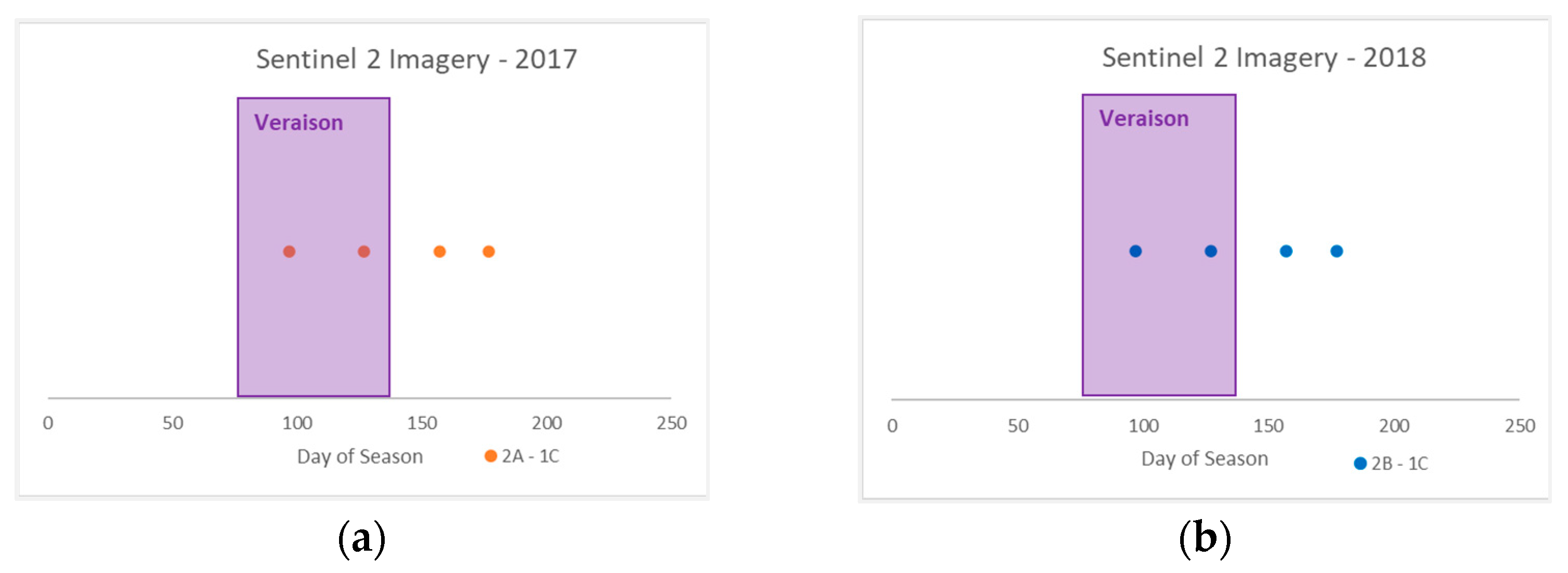
The Sentinel-2 constellation is formed by 2 satellites in heliosynchronous orbit with a temporal resolution of 10 days for each satellite, or 5 altogether. Both satellites carry a multispectral image sensor (MSI) able to acquire images in 13 spectral bands, from 433 nm to 2280 nm. The red (665 nm) and near infrared (842 nm) bands are of particular interest for agricultural applications, since they allow for the calculation of several vegetation indices at a 10 m spatial resolution [41]. The productive cycle of the grapevine has several phases: pruning, weeping, budding, flowering, fruit set, veraison, maturity and leaf fall. The budding phase, in which new stems appear and the first leaves appear, occurs in the first fortnight of October; therefore, the date of the beginning of the season was established as 15 October. Figure 3 shows the acquisition date of a set of 8 images used in this work for the two years of study, referred to the day of the season (DOS).
To establish the ripening of the plots, a total of 14 grape samples were collected in the field after veraison. The location of the sampling points was established by identifying strategic and homogeneous response areas. Zones that share common characteristics of vegetative expression and topography were selected, and the samples were homogeneously distributed in the plots. A sample was positioned in each plot except for plot 7.08, which presents two sampling positions, which were averaged (Figure 1). These positions were considered to carry out the micro-vinification in which phenols, anthocyanins and color intensity were measured.
3. Methods
3.1. Satellite Data Preparation
Sentinel images were co-registered using ground control points and applying the nearest neighbor resampling method preserving the original pixel size. Eight of the thirteen Sentinel-2 bands were used, corresponding to B3 (Green band—centered on 0.560 µm), B4 (Red band—0.665 µm), B5 (Red Edge band—0.705 µm), B6 (Red Edge band—0.740 µm), B7 (Red Edge band—0.783 µm), B8 (NIR band—0.842 µm), B11 (SWIR band 1—1.610 µm) and B12 (SWIR band 2—2.190 µm). Four spectral indices were calculated: Green Normalized Difference Vegetation Index (GNDVI), Normalized Difference Vegetation Index (NDVI), Normalized Difference Moisture Index (NDMI) and Chlorophyll Index.
The term vegetation index refers to any transformation of two or more spectral bands for assessing vegetation properties either at the leaf or canopy levels, developed for different types of vegetation [42].
NDVI ((NIR − Red)/(NIR + Red)) is a simple indicator closely related to crop vegetative and productive features [30]. GNDVI ((NIR − Green)/(NIR + Green)) is a variant of NDVI more sensitive to water and nitrogen uptake into the plant canopy [18]. In the case of the Chlorophyll Index ((Red − Blue)/Green), the effect of photosynthetic pigments is dominating the reflectance in the visible spectral region [42]. Carotenoids contribute to strong absorption at 445 nm, anthocyanin at 529 nm and chlorophyll at 650 nm [43]. The NDMI ((NIR − SWIR1)/(NIR + SWIR1)) is sensitive to the moisture content in the canopy [44]. The SWIR1 band corresponds to the wavelength comparatively more similar to the Landsat shortwave band, the base of this indicator [45,46,47,48].
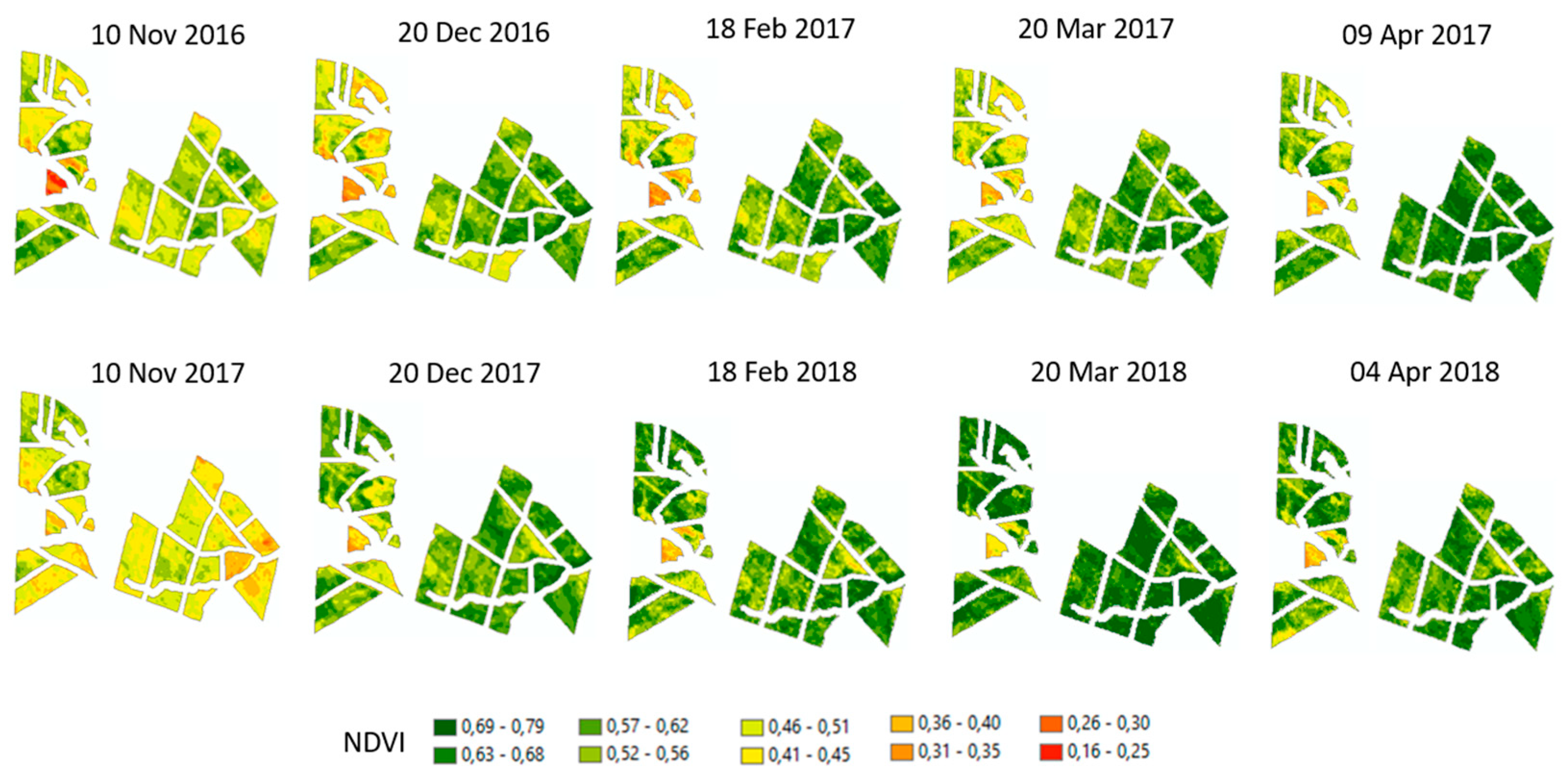
The visualization of the behavior and evolution of the vineyard allows to overview the state of the plots and the development in both seasons. For this purpose, the NDVI was used, since this is considered an indicator related to the quantity, quality and state of vegetation [48]. The best vegetative expression, or the maximum potential of NDVI, occurs in summer shortly before the veraison, since just after this, the foliage begins to change, and near the harvest the vines begin to lose their leaves. The development cycle of the vines begins with pruning and new plantings in July/August, and then starts the flowering in August/September, budding in September/October, flowering in October/November, fruit set in November/December, veraison in January/February and finally the harvest in March/April. Therefore, to characterize the entire cycle of each season, the set of NDVI images used was from September to April.
Figure 4 shows the NDVI maps displayed on a 10-rank scale. The plots are grouped by year of planting, 2007 and 2010. The 2007 plantation, located north, is made up of 12 plots and the 2010 plantation, located south, by 11 plots. In order to avoid mixed pixels in the boundary of the plots, a buffer of 15 m was applied.
3.2. Samples and Micro-Vinification
A Unicam Helios Gamma 9423 1000E spectrophotometer was used to measure both color intensity and phenolic compounds in general. Due to the wide chemical diversity of phenolic compounds, total phenols in must and wines are generally presented in arbitrary units of a phenolic standard, such as the amount of gallic acid needed to produce the same analytical response or gallic acid equivalents [5], as was performed in this case. When measuring the phenolic compounds with spectrophotometers, no specific compounds but rather total compounds are measured, which are expressed on the basis of the specific compounds that recur most frequently among phenols and anthocyanins.
The method for measuring total phenols was measuring absorbance at 280 nm (a gallic acid calibration curve was used). The measurement of the total anthocyanins was carried out by decolorization and measured at 520 nm. The method to measure color intensity was the Glories method, which corresponds to the sum of the absorbances at 420 nm, 520 nm and 620 nm [49].
Micro-vinification was made from the abovementioned 14 field samples. Approximately 1000 kg of grapes per micro-vinification were crushed and blended to enter the alcoholic fermentation process and this ended when 2 g of sugar per liter was reached. The wine was then transferred to barrels. Then came malolactic fermentation, which was carried out in a heated place to increase the speed of fermentation.
3.3. Oenological Evaluation
Since phenolic compounds are important in the overall quality of wine, they are the subject of intense research worldwide [6]. They provide sensory characteristics such as flavor, aroma, color, and astringency, among others [31].
Viña Montes evaluates wines in three categories: Limited (LIM), Premiun (PRE) and Superior (SPR). Each of these has three variants with a lower (−) and a higher (+) subcategory, indicating that a taster can evaluate a wine as Premium, but below or above the average of this category.
The factors used to evaluate the wines were as follows: (i) Visual factors: mainly associated with color; therefore, anthocyanins and color intensity will predominate them. Cleanliness was also observed (cloudy, clear, clean, bright, etc.), which is associated to physicochemical stability. Color intensity varies according to the grape variety but seeks to identify colorimetric intensities such as red, intense red, ruby red, violet, intense violet, etc. (ii) Olfactory factors: associated with volatile properties and it is described through aromas (wood, vanilla, fruits, etc.). The greater the number of descriptors and complexity, the higher the classification of a wine. (iii) Flavor factors: tannins, compounds found in the skin and seeds of berries, which produce the sensation of astringency. Not only a high concentration of tannins is sought, but they must be of good sensory quality. Together with the alcohol, they confer the sensation of structure and body. A wine with more body and better structure is classified as superior quality. (iv) Finish of a wine: indicates a higher or lower category; the finish is the persistence of a wine in the mouth, so a wine with a persistent, long, medium or short finish is also a factor associated with categories.
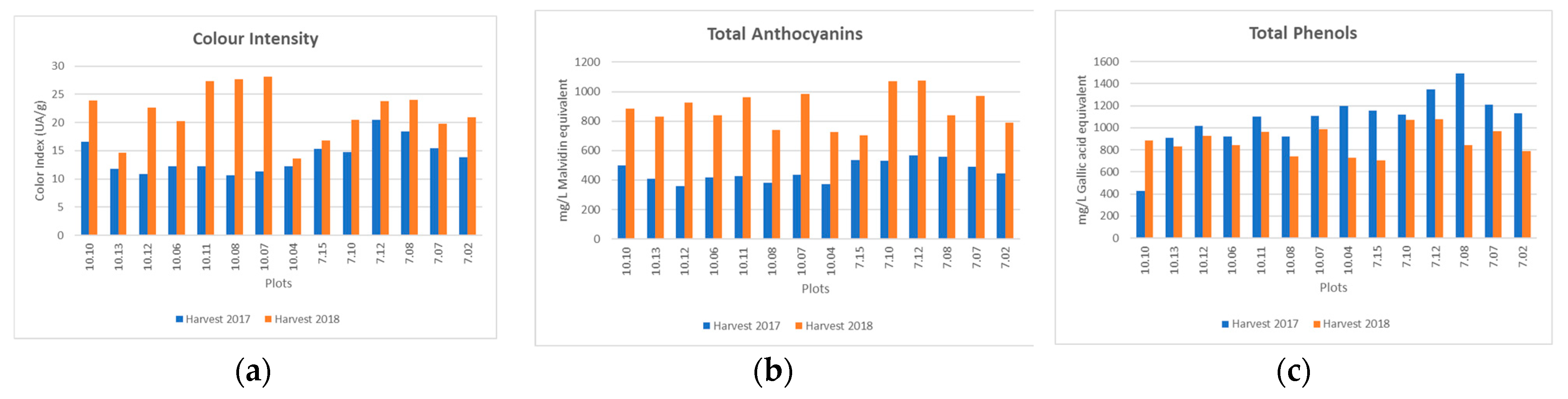
Attending to these factors, each wine sample was evaluated by four winemakers who assigned an individual evaluation. Then, they were averaged to give a final category to each sample. Table 1 shows the final quality category assigned to each plot and the color intensity value, total phenolic compounds and anthocyanins measured with the spectrophotometer. Figure 5 shows the comparison of the quality factors in the two seasons.
3.4. Modeling Phenolic Compounds (PC) and Color Intensity (CI)
The modeling of the variables requires the values measured in the micro-vinification and the response of the foliage that will be reflected in the spectral bands and indices. Since the variables are obtained post-harvest, it will be necessary to know the relationship between the samples and the series of images to represent the vegetative expression from veraison to harvest. The average value of pixels considered as representative of the images was taken to the set of pixels within a 15 m radius around the location corresponding to the sampling and micro-vinification (Figure 1).
For each sampling point a table was prepared, including the name of the plot, the values obtained in the microvinification corresponding to total phenols (TP), the total anthocyanins (AT) and the color intensity (CI), which were used as the dependent variables. Similarly, the independent variables correspond to the average value of pixels around the sample in the original Sentinel 2 bands and in the four spectral indices, on the four dates of each season, from January to April. A multiple ordinary linear regression model was used to determine the relationship between the image-derived data and the variables (phenolic compounds and color intensity).
To select the best model, a descriptive analysis of the variables was carried out, for which the correlation matrix of the bands on the different dates was reviewed. In order to identify the strength of the linear relationship between the variables, as well as the statistical significance of the estimated correlations, a confidence level of 95% was considered; therefore, p-values less than 0.05 will be sought.
To avoid severe multicollinearity between the variables, variance inflation factors (VIF) were considered, which allow measuring the correlation between the predictor variables of the model.
Ordinary multiple linear regression models were used to find the best coefficient of determination (R2) between January and April. To do this, the best combination of variables or the variable that was significant both for the model and individually was selected, followed by the collinearity check of the variables using the variance inflation factor (VIF).
4. Results
The selected models included only 1 or 2 variables. Some models composed of variables with a high degree of significance and a slight degree of collinearity were retained (e.g., CI February 2017), as well as one of the models with low collinearity that included a variable with a p-value greater than 0.05 (TP April 2017).
During the 2017 season, color intensity presented high R2 values for the four dates, April being the best of them, as well as the results for total anthocyanins. In both variables, during the 2018 season, the models reached very low R2 values. The mean absolute error (MAE) corresponding to the average value of the residuals was higher in the 2018 season. The total phenols variable presented more similar errors in both seasons and reached a better R2 in the 2018 season, February being the best of them.
Table 2 shows the summary statistics for each dependent variable for the four dates under study—color intensity (CI), total phenols (TP), total anthocyanins (TA)—including the coefficient of determination (R2), the variables included in each model, their mean absolute error (MAE), the variance inflation factor (VIF) and the significance (p-value) for the model and the individual variables, which constitute all the information necessary to select the month with the best indicators.
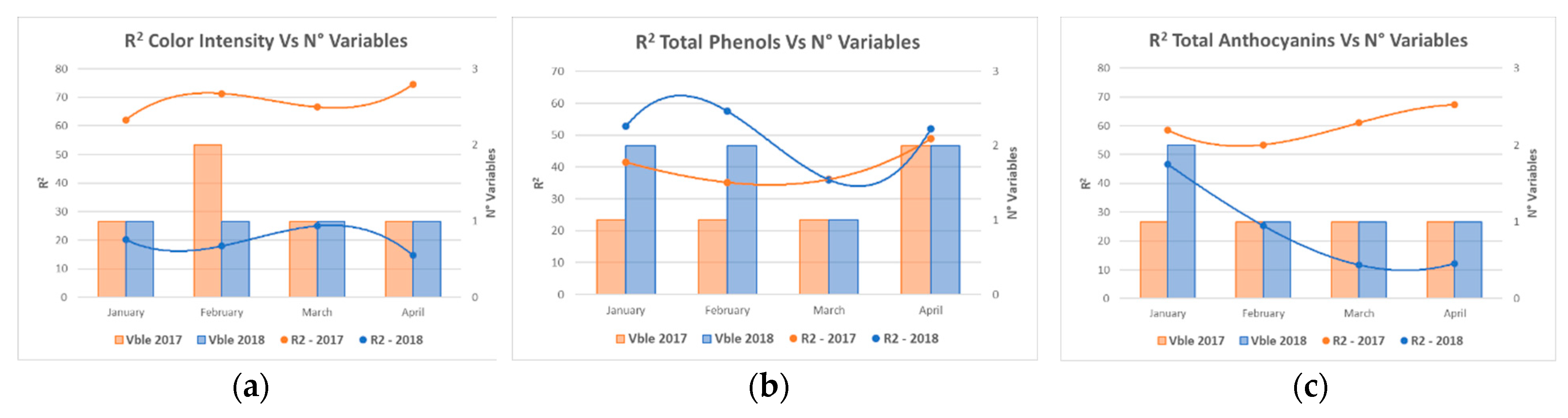
Considering the small number of samples studied and in order to avoid using variables with high collinearity, those models with VIF values less than 10 were chosen. Figure 6 shows the coefficient of determination obtained at each date and the number of variables included in the model.
Attending to the results obtained, April is the best month to predict the intensity of the coloration and anthocyanins, unlike phenols, whose best R2 is presented in February.
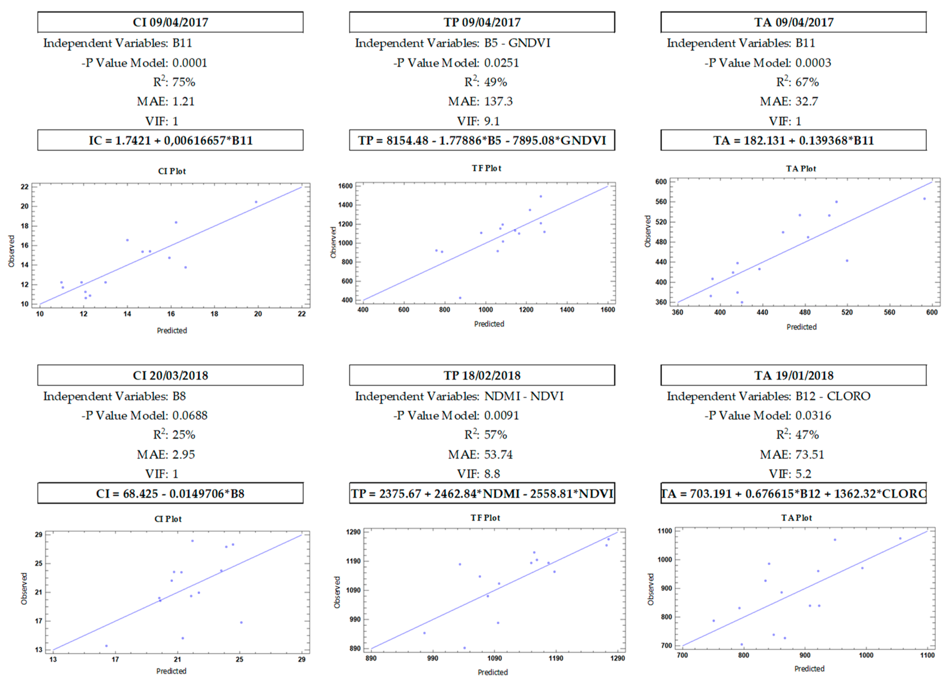
A summary of the complete statistics of the selected models as well as a scatter plot of the individual models, including the equations of the models in both seasons for the three dependent variables, color intensity (CI), total phenols (TP) and total anthocyanins (TA), are shown in the Figure 7.
As shown in Figure 7, variables are not repeated in the models with respect to the comparison by variable between the two years. The 2017 season presents two models with one variable (CI and TA) and TP with two variables. In the case of the 2018 season, only CI is selected with one variable and TP and TA with two variables. Regarding the coefficients of determination, only the 2017 season shows reliable models above 60%.
Since these models are different depending on the date, their precision is limited in time, which implies that they should be obtained monthly. Although the study brings us closer to a date in which the greatest relationship occurs, the moment could vary slightly in each campaign, due to external factors such as the meteorological conditions. This temporal limitation does not restrict the benefits of this tool in the objective of this study, since these models would serve to identify the zoning where the next sampling or field visit will take place. This would contribute to carry out the harvest differentiation within a plot, allowing to improve the determination of the maturity and optimize the harvest moment in each plot.
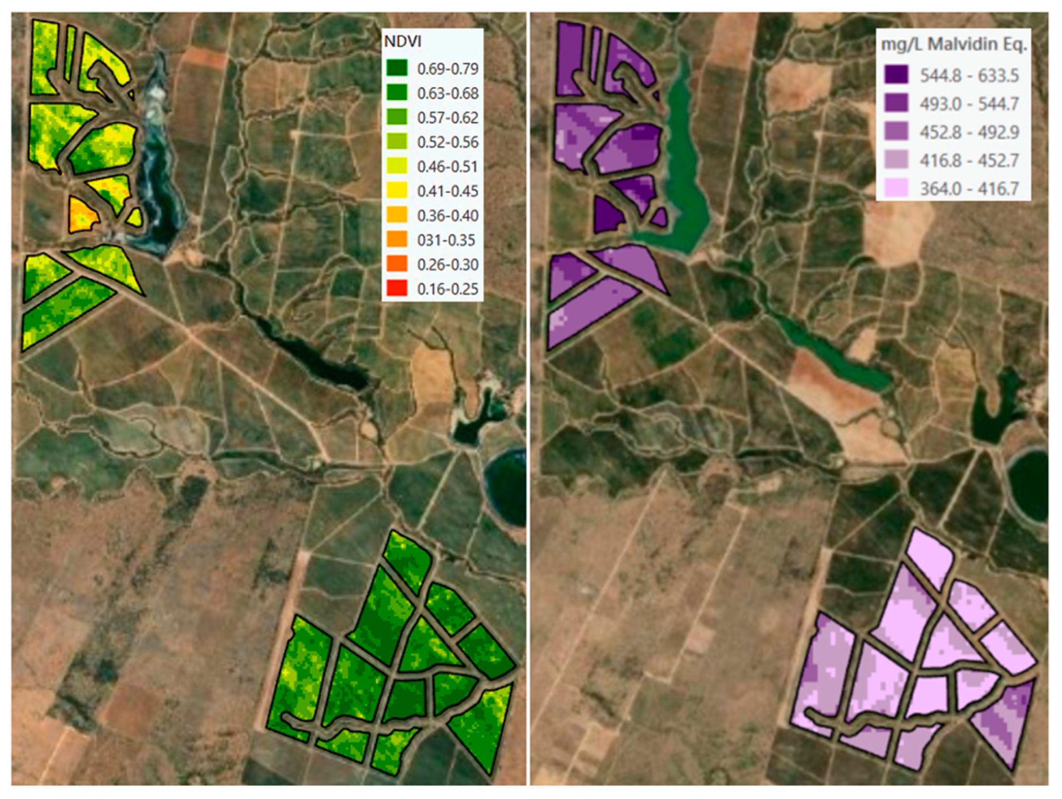
By applying phenolic compounds and color intensity estimation models, it is possible to obtain representative maps of the quality status at a given date, showing the variability of each plot in terms of the ripening potential represented by the canopy. This would allow, through the use of a limited number of field samples and Sentinel-2 images, to estimate these wine quality variables in the entire plot and, subsequently, to identify ripeness variability and zonation to determine a selective harvesting.
Figure 8 shows comparative maps between the NDVI and estimated total anthocyanins. In agreement with Cortell et al. (2007) [50], who determined that vines with low vigor show higher levels of anthocyanin and flavanol in the grape skin, an inverse relationship between the estimated anthocyanins and NDVI can be noticed.
5. Discussion
Defining the quality of wine is relative; however, there are some standard variables to determine the technological maturity (state of greater accumulation of sugar and low acidity), phenolic maturity responsible for the color of the berries [51], sensorial characteristics, such as color, astringency and bitterness, and aging capacity, which are closely related to the perception of wine quality [52]. For this purpose, it is key to consider the variability of a parcel, since the mixture of grapes from different quality indicators do not result in an intermediate quality wine, since some properties found in low-quality grapes (immature phenolic compounds, herbaceous aromas, etc.) prevail in the wine even when a small proportion of grapes with those characteristics are present [53]. All these considerations are key in the quality of wine, allowing a better use of resources from an environmental and food safety point of view [54].
Our results show that during the 2017 season, the R2 values of the studied quality parameters are better starting in April. The results obtained in both seasons do not allow to establish a common pattern of behavior in both seasons. This difference is appreciated in the comparison of the values obtained in the microvinification; in the case of anthocyanins, in some lots the content practically doubles, not a very strange condition if we consider that the typical concentrations of free anthocyanins in full-bodied young red wines are around 500 mg/L, but in some cases can be higher than 2000 mg/L [55,56,57,58].
Several studies have established that anthocyanins begin to be produced more intensely from veraison onwards [58], but the process is complex as it is affected by multiple factors that could affect berry composition and anthocyanin accumulation, such as environmental conditions [59] and agricultural management [60]. These factors can significantly influence the anthocyanin content of grapes [61]. For example, water deficit has been shown to have a positive effect on anthocyanin accumulation during ripening [62,63] and others have shown that water limitation has negative effects [59,64].
The fact that the highest modelling potential of phenolic compounds occur later in 2017 may be justified by the study of Mori et al. (2007) who showed that high temperatures reduced the total anthocyanin content to less than half of what was expected [64]. A number of other studies agree that temperature is a critical variable in the final amount of anthocyanins present in wine [6,65,66]. The comparison of the analysis of the micro-vinifications for both seasons shows higher absorbance values for both color intensity and phenolic compounds for the 2018 season, in agreement with other studies that obtained better results with cooler temperatures [66]. This seems to be one of the key factors to consider [67], since vegetative growth and phenolic compound synthesis are affected by temperature [68]. Global warming produces an increase in the gap between technological maturity, corresponding to the stage of higher sugar accumulation and low acidity (which comes earlier) and phenolic and aromatic maturity (which comes later) [69,70] which is ratified by the results obtained in this study, where the best correlations occur in April the first season (warmer). These works suggest the convenience to include temperature variables in the models, which could eventually improve the results obtained.
The study of the variables directly involved in wine quality, such as phenolic compounds and color, contributes to the interest of researchers to delve into studies of nondestructive and affordable techniques based on the use of satellite images that allow understanding the factors that determine the concentration of these quality variables. These models might be useful for the differentiated management of harvests, providing spatial information for selective harvesting, which could be used to categorize different types of wine, and might be complemented with the very extensive information that is progressively available in a vineyard, related to agronomic management, such as nutrition, thinning, leaf removal and grafting, among others.
6. Conclusions
The purpose of this research was to determine models from Sentinel-2 image series that allow estimating, prior to harvest, wine quality variables such as phenols (TP), anthocyanins (TA) and color intensity (CI). These variables provide sensory characteristics that are evaluated in the wine. Two harvest seasons were studied and models with R2 coefficients of determination above 60% were obtained for CI in 2017 (75%) and TA in 2017, at 67%. These results transform the estimated TP, TA and CI maps into a useful tool, with the potential to define selective harvests.
Sentinel 2 images play a key role, as their high periodicity allows modeling of pre-harvest vine conditions. The final stage of ripening and the harvest time is a very short but strategic stretch that would allow identifying homogeneous sectors for harvesting and thus scheduling the winery space.
The results also show the convenience to deepen this study on two specific aspects in the future: (i) to increase the number of samples to improve the dispersion and variety of the data; and (ii) to include a climatic variable, such as cumulative temperature, which could help in understanding the behavior of phenolic compounds and the changes in color in order to obtain more robust models.
The optimization of all processes in the wine production chain aims to raise the quality level of winemaking. Therefore, the production of maps that allows spatially differentiating the variability and quality potential of wine produced in terms of color intensity and phenolic compounds accumulation presents a practical and attractive potential to identify aging capacity and the style of wine expected from different plots as well as their productive aptitude. This work suggests that remote sensing and selective harvesting can be used to better manage the style and quality of wine produced.
Author Contributions
Conceptualization, S.N.F., L.Á.R. and J.A.R.; methodology, S.N.F., L.Á.R. and J.A.R.; investigation, S.N.F.; writing—original draft preparation, S.N.F.; writing—review and editing, S.N.F., L.Á.R. and J.A.R.; supervision, L.Á.R. and J.A.R. All authors have read and agreed to the published version of the manuscript.
Funding
This research received no external funding.
Institutional Review Board Statement
Not applicable.
Informed Consent Statement
Not applicable.
Data Availability Statement
This study do not report any data.
Acknowledgments
We gratefully acknowledge the valuable contribution, knowledge and generosity of Rodrigo Opazo, agronomist engineer of Viña Montes, as well as Rodrigo Barria, agronomist and manager, who authorized the acquisition of samples and use of the laboratory and facilities of Viña Montes that made this study possible.
Conflicts of Interest
The authors declare no conflict of interest.
References
- Matese, A.; Di Gennaro, S.F. Technology in precision viticulture: A state of the art review. Int. J. Wine Res. 2015, 7, 69–81. [Google Scholar] [CrossRef] [Green Version]
- del Valle Fernandez, M.; Peña, I.; Sanchez de Pablo, J.D. Factors of competitiveness in the wine industry: An analysis of innovation strategy. World Acad. Sci. Eng. Technol. 2011, 78, 503–513. [Google Scholar] [CrossRef]
- Vidal, S.; Francis, L.; Noble, A.; Kwiatkowski, M.; Cheynier, V.; Waters, E. Taste and mouth-feel properties of different types of tannin-like polyphenolic compounds and anthocyanins in wine. Anal. Chim. Acta 2004, 513, 57–65. [Google Scholar] [CrossRef]
- Wrolstad, R.E.; Durst, R.W.; Lee, J. Tracking color and pigment changes in anthocyanin products. Trends Food Sci. Technol. 2005, 16, 423–428. [Google Scholar] [CrossRef]
- Zoecklein, B.W.; Fugelsang, K.C.; Gump, B.H.; Nury, F.S. Phenolic Compounds and Wine Color. Wine Anal. Prod. 1995, 115–151. [Google Scholar] [CrossRef]
- Kennedy, J.A. Grape and wine phenolics: Observations and recent findings. Cienc. Investig. Agrar. 2008, 35, 107–120. [Google Scholar] [CrossRef]
- Jackson, M.G.; Timberlake, C.F.; Bridle, P.; Vallis, L. Red wine quality: Correlations between colour, aroma and flavour and pigment and other parameters of young Beaujolais. J. Sci. Food Agric. 1978, 29, 715–727. [Google Scholar] [CrossRef]
- Casassa, F.; Sari, S. Aplicación del Sistema Cie-Lab a Los Vinos Tintos. Correlación con Algunos Parámetros Tradicionales. Rev. Enol. 2006, 3, 10. Available online: http://www.researchgate.net/profile/L_Casassa/publication/ (accessed on 25 November 2021).
- Busse-Valverde, N.; Gómez-Plaza, E.; López-Roca, J.M.; Gil-Muñoz, R.; Bautista-Ortín, A.B. The Extraction of Anthocyanins and Proanthocyanidins from Grapes to Wine during Fermentative Maceration Is Affected by the Enological Technique. J. Agric. Food Chem. 2011, 59, 5450–5455. [Google Scholar] [CrossRef] [PubMed]
- Gabrielyan, A.; Kazumyan, K. The investigation of phenolic compounds and anthocyanins of wines made of the grape variety karmrahyut. Ann. Agrar. Sci. 2018, 16, 160–162. [Google Scholar] [CrossRef]
- Esparza, I.; Santamaría, C.; Fernández, J. Chromatic characterisation of three consecutive vintages of Vitis vinifera red wine: Effect of dilution and iron addition. Anal. Chim. Acta 2006, 563, 331–337. [Google Scholar] [CrossRef] [Green Version]
- Programa Territorial Integrado, Vinos de Chile 2010. “Monitoreo de Madurez”. Centro Tecnologico de la Vid y El Vino. 2010. Available online: http://static.elmercurio.cl/Documentos/Campo/2012/11/19/20121119153346.pdf (accessed on 20 November 2021).
- Castro, A.L. Efecto del Momento de Cosecha de Uva cv. Merlot Cobre la Composicion Quimica y Sensorial de los Vinos en el Valle del Maipo; Universidad de Chile: Santiago, Chile, 2005. [Google Scholar]
- Vélez, S.; Rubio, J.A.; Andrés, M.I.; Barajas, E. Agronomic classification between vineyards (‘Verdejo’) using NDVI and Sen-tinel-2 and evaluation of their wines. Vitis J. Grapevine Res. 2019, 58, 33–38. [Google Scholar] [CrossRef]
- Hall, A.; Louis, J.; Lamb, D. Characterising and mapping vineyard canopy using high-spatial-resolution aerial multispectral images. Comput. Geosci. 2003, 29, 813–822. [Google Scholar] [CrossRef]
- Cortell, J.M.; Halbleib, M.; Gallagher, A.V.; Righetti, A.T.L.; Kennedy, J.A. Influence of Vine Vigor on Grape (Vitis vinifera L. Cv. Pinot Noir) and Wine Proanthocyanidins. J. Agric. Food Chem. 2005, 53, 5798–5808. [Google Scholar] [CrossRef]
- Soubry, I.; Patias, P.; Tsioukas, V. Monitoring vineyards with UAV and multi-sensors for the assessment of water stress and grape maturity. J. Unmanned Veh. Syst. 2017, 5, 37–50. [Google Scholar] [CrossRef] [Green Version]
- Fredes, S.; Ruiz, L.; Recio, J. Modeling° Brix and pH in Wine Grapes from Satellite Images in Colchagua Valley, Chile. Agriculture 2021, 11, 697. [Google Scholar] [CrossRef]
- Martínez-Casasnovas, M.C.; Agelet, J.A.; Arnó, J.; Bordes, J.; Ramos, X. Protocolo para la Zonificación Intraparcelaria de la Viña para Vendimia Selectiva a partir de Imágenes Multiespectrales. Rev. Teledetec. 2010, 33, 47–52. [Google Scholar]
- Johnson, L.; Roczen, D.; Youkhana, S.; Nemani, R.; Bosch, D. Mapping vineyard leaf area with multispectral satellite imagery. Comput. Electron. Agric. 2003, 38, 33–44. [Google Scholar] [CrossRef]
- Cunha, M.; Marcal, A.R.S.; Silva, L. Very early prediction of wine yield based on satellite data from vegetation. Int. J. Remote Sens. 2010, 31, 3125–3142. [Google Scholar] [CrossRef]
- Martinez-Casasnovas, J.A.; Agelet-Fernandez, J.; Arnó, J.; Ramos, M.C. Analysis of vineyard differential management zones and relation to vine development, grape maturity and quality. Span. J. Agric. Res. 2012, 10, 326. [Google Scholar] [CrossRef] [Green Version]
- Sun, L.; Gao, F.; Anderson, M.C.; Kustas, W.P.; Alsina, M.M.; Sanchez, L.; Sams, B.; McKee, L.; Dulaney, W.; White, W.A.; et al. Daily Mapping of 30 m LAI and NDVI for Grape Yield Prediction in California Vineyards. Remote Sens. 2017, 9, 317. [Google Scholar] [CrossRef] [Green Version]
- Lamb, D.; Weedon, M.; Bramley, R. Using remote sensing to predict grape phenolics and colour at harvest in a Cabernet Sauvignon vineyard: Timing observations against vine phenology and optimising image resolution. Aust. J. Grape Wine Res. 2008, 10, 46–54. [Google Scholar] [CrossRef] [Green Version]
- Edo-Roca, M.; Nadal, M.; Lampreave, M. How terroir affects bunch uniformity, ripening and berry composition in Vitis vinifera cvs. Carignan and Grenache. J. Int. Sci. Vigne 2013, 47, 1–20. [Google Scholar] [CrossRef]
- Martínez-Gil, A.M.; Gamboa, G.G.; Garde-Cerdán, T.; Pérez-Álvarez, E.P.; Moreno-Simunovic, Y. Characterization of phenolic composition in Carignan noir grapes (Vitis vinifera L.) from six wine-growing sites in Maule Valley, Chile. J. Sci. Food Agric. 2018, 98, 274–282. [Google Scholar] [CrossRef] [PubMed]
- Arnó, J.; Casasnovas, J.M.; Ribes-Dasi, M.; Rosell-Polo, J.R. Review. Precision viticulture. Research topics, challenges and opportunities in site-specific vineyard management. Span. J. Agric. Res. 2009, 7, 779. [Google Scholar] [CrossRef] [Green Version]
- Urretavizcaya, I.; Santesteban, L.G.; Tisseyre, B.; Guillaume, S.; Miranda, C.; Royo, J.B. Oenological significance of vineyard management zones delineated using early grape sampling. Precis. Agric. 2013, 15, 130–131. [Google Scholar] [CrossRef] [Green Version]
- Perez Quezada, J. Viticultura de Precisión Aplicada Al Viñedo. Rev. Enol. 2006, 2, 1–3. [Google Scholar]
- Khaliq, A.; Comba, L.; Biglia, A.; Ricauda Aimonino, D.; Chiaberge, M.; Gay, P. Comparison of Satellite and UAV-Based Multispectral Imagery for Vineyard Variability Assessment. Remote Sens. 2019, 11, 436. [Google Scholar] [CrossRef] [Green Version]
- Duran, O.D.; Trujillo, N.Y. Estudio Comparativo del Contenido Fenólico de Vinos Tintos Colombianos e Importados. Vitae 2008, 15, 17–24. [Google Scholar]
- Lima, L.J. Estudio De Caracterización De La Cadena De Producción Y Comercialización De La Agroindustria Vitivinícola: Estructura, Agentes Y Prácticas. Of. Estud. Políticas Agrar. Minist. Agric 2015, 208. Available online: http://www.odepa.gob.cl (accessed on 25 November 2021).
- Bramley, R. Precision Viticulture: Managing Vineyard Variability for Improved Quality Outcomes; Woodhead Publishing: Cambridge, UK, 1999; pp. 445–480. [Google Scholar]
- Chaves, M.M.; Harley, P.C.; Tenhunen, J.D.; Lange, O.L. Gas exchange studies in two Portuguese grapevine cultivars. Physiol. Plant. 1987, 70, 639–647. [Google Scholar] [CrossRef]
- Müller, K. Chile vitivinícola en pocas palabras. Rev. Enol. 2004. Available online: http://www.acenologia.com/ciencia69_01.htm (accessed on 20 November 2021).
- Parpinello, G.P.; Ricci, A.; Arapitsas, P.; Curioni, A.; Moio, L.; Riosegade, S.; Ugliano, M.; Versari, A. Multivariate characterisation of Italian monovarietal red wines using MIR spectroscopy. OENO One 2019, 53, 741–751. [Google Scholar] [CrossRef] [Green Version]
- Merkytė, V.; Longo, E.; Windisch, G.; Boselli, E. Phenolic Compounds as Markers of Wine Quality and Authenticity. Foods 2020, 9, 1785. [Google Scholar] [CrossRef] [PubMed]
- Uribe, A.; Catalan, H. Caracterización Hidroclimatológica y del uso de suelo del Secano de la Región de O’higgins; Boletin INIA-Instituto de Investigaciones Agropecuarias: Punta Arenas, Chile, 2016; Volume 1, pp. 49–81. [Google Scholar]
- Giraldo, C. Escenarios de la Vitivinicultura Chilena Generados por los Cambios en la Aptitud Productiva, como Consecuencia del Cambio Climatico para Mediados del siglo XX1; Univerisdad de Chile: Santiago, Chile, 2017. [Google Scholar]
- Pardo, J.A. Seguimiento Fenologico del Cultivo de Uva Isabela (Vitis sp.) en Fusagasuga Cundinamarca; Universidad de Cundinamarca: Fusagasugá, Columbia, 2016. [Google Scholar]
- Sozzi, M.; Kayad, A.; Marinello, F.; Taylor, J.; Tisseyre, B. Comparing vineyard imagery acquired from Sentinel-2 and Unmanned Aerial Vehicle (UAV) platform. OENO One 2020, 54, 189–197. [Google Scholar] [CrossRef] [Green Version]
- Hallik, L.; Kazantsev, T.; Kuusk, A.; Galmés, J.; Tomás, M.; Niinemets, Ü. Generality of relationships between leaf pigment contents and spectral vegetation indices in Mallorca (Spain). Reg. Environ. Chang. 2017, 17, 2097–2109. [Google Scholar] [CrossRef]
- Sims, D.A.; Gamon, J.A. Relationships between leaf pigment content and spectral reflectance across a wide range of species, leaf structures and developmental stages. Remote Sens. Environ. 2002, 81, 337–354. [Google Scholar] [CrossRef]
- Herrera, M.; Chuvieco, E. Estimación del contenido de agua a partir de mediciones hiperespectrales para cartografía del riesgo de incendio. Cuad. Investig. Geográfica 2014, 40, 295–310. [Google Scholar] [CrossRef] [Green Version]
- Gao, B.-C. NDWI a Normalized Difference Water Index for Remote Sensing of Vegetation Liquid Water from Space; Elsevier: Amsterdam, The Netherlands, 1996; Volume 23, pp. 257–266. [Google Scholar] [CrossRef] [Green Version]
- Wang, L.; Qu, J.J.; Hao, X.; Hunt, E.R. Estimating dry matter content from spectral reflectance for green leaves of different species. Int. J. Remote Sens. 2011, 32, 7097–7109. [Google Scholar] [CrossRef]
- Wang, L.; Hunt, E.R.; Qu, J.J.; Hao, X.; Daughtry, C. Remote sensing of fuel moisture content from ratios of narrow-band vegetation water and dry-matter indices. Remote Sens. Environ. 2013, 129, 103–110. [Google Scholar] [CrossRef] [Green Version]
- Hernández, C.; Escribano, J.; Tarquis, A. Comparación del Índice de Vegetación de Diferencia Normalizada obtenido a diferentes escalas en pastos de Dehesa. In Proceedings of the 53ª Reunión Científica de la SEEP, Madrid, Spain, 9–12 June 2014; pp. 121–128. [Google Scholar]
- Opazo, R. Protocolo Fenoles Totales; Marchigue, Colchagua; 2017; p. 1. [Google Scholar]
- Cortell, J.M.; Halbleib, M.; Gallagher, A.V.; Righetti, T.L.; Kennedy, J.A. Influence of Vine Vigor on Grape (Vitis vinifera L. Cv. Pinot Noir) Anthocyanins. 1. Anthocyanin Concentration and Composition in Fruit. J. Agric. Food Chem. 2007, 55, 6575–6584. [Google Scholar] [CrossRef]
- Peña, A. Factores que Regulan el Color en Uvas Tintas. 2005, pp. 12–14. Available online: http://www.gie.uchile.cl/pdf/Alvaro%20Pe%F1a/Color%20de%20las%20bayas.pdf (accessed on 20 November 2021).
- Jaffré, J.; Valentin, D.; Dacremont, C.; Peyron, D. Burgundy red wines: Representation of potential for aging. Food Qual. Prefer. 2009, 20, 505–513. [Google Scholar] [CrossRef]
- Kontoudakis, N.; Esteruelas, M.; Fort, F.; Canals, J.-M.; Freitas, V.; Zamora, F. Influence of the heterogeneity of grape phenolic maturity on wine composition and quality. Food Chem. 2011, 124, 767–774. [Google Scholar] [CrossRef]
- Gebbers, R.; Adamchuk, V.I. Precision Agriculture and Food Security. Science 2010, 327, 828–831. [Google Scholar] [CrossRef] [PubMed]
- Mulinacci, N.; Santamaria, A.; Giaccherini, C.; Innocenti, M.; Valletta, A.; Ciolfi, G.; Pasqua, G. Anthocyanins and flavan-3-ols from grapes and wines of Vitis vinifera cv. Cesanese d’Affile. Nat. Prod. Res. 2008, 22, 1033–1039. [Google Scholar] [CrossRef]
- Pour Nikfardjam, M.S.; Márk, L.; Avar, P.; Figler, M.; Ohmacht, R. Polyphenols, anthocyanins, and trans-resveratrol in red wines from the Hungarian Villány region. Food Chem. 2006, 98, 453–462. [Google Scholar] [CrossRef]
- He, F.; Liang, N.-N.; Mu, L.; Pan, Q.-H.; Wang, J.; Reeves, M.J.; Duan, C.-Q. Anthocyanins and Their Variation in Red Wines I. Monomeric Anthocyanins and Their Color Expression. Molecules 2012, 17, 1571–1601. [Google Scholar] [CrossRef] [PubMed] [Green Version]
- Teixeira, A.; Eiras-Dias, J.; Castellarin, S.D.; Gerós, H. Berry Phenolics of Grapevine under Challenging Environments. Int. J. Mol. Sci. 2013, 14, 18711–18739. [Google Scholar] [CrossRef] [PubMed] [Green Version]
- Bucchetti, B.; Matthews, M.A.; Falginella, L.; Peterlunger, E.; Castellarin, S.D. Effect of water deficit on Merlot grape tannins and anthocyanins across four seasons. Sci. Hortic. 2011, 128, 297–305. [Google Scholar] [CrossRef]
- Kyraleou, M.; Koundouras, S.; Kallithraka, S.; Theodorou, N.; Proxenia, N.; Kotseridis, Y. Effect of irrigation regime on anthocyanin content and antioxidant activity of Vitis vinifera L. cv. Syrah grapes under semiarid conditions. J. Sci. Food Agric. 2016, 96, 988–996. [Google Scholar] [CrossRef] [PubMed]
- Theodorou, N.; Nikolaou, N.; Zioziou, E.; Kyraleou, M.; Kallithraka, S.; Kotseridis, Y.; Koundouras, S. Anthocyanin content and composition in four red winegrape cultivars (Vitis vinifera L.) under variable irrigation. OENO One 2019, 53, 39–51. [Google Scholar] [CrossRef]
- Zarrouk, O.; Francisco, R.; Pintó-Marijuan, M.; Brossa, R.; Santos, R.R.; Pinheiro, C.; Costa, J.; Lopes, C.; Chaves, M.M. Impact of irrigation regime on berry development and flavonoids composition in Aragonez (Syn. Tempranillo) grapevine. Agric. Water Manag. 2012, 114, 18–29. [Google Scholar] [CrossRef]
- Arrizabalaga, M.; Morales, F.; Oyarzun, M.; Delrot, S.; Gomès, E.; Irigoyen, J.J.; Hilbert, G.; Pascual, I. Tempranillo clones differ in the response of berry sugar and anthocyanin accumulation to elevated temperature. Plant Sci. 2018, 267, 74–83. [Google Scholar] [CrossRef] [PubMed]
- Mori, K.; Goto-Yamamoto, N.; Kitayama, M.; Hashizume, K. Loss of anthocyanins in red-wine grape under high temperature. J. Exp. Bot. 2007, 58, 1935–1945. [Google Scholar] [CrossRef]
- Coombe, B.G.; McCarthy, M.G. Dynamics of grape berry growth and physiology of ripening. Aust. J. Grape Wine Res. 2000, 6, 131–135. [Google Scholar] [CrossRef]
- Del Valle, R.; Gonzalez, G.; Baez, A. Antocianinas en uva (Vitis vinifera L.) y su relación con el color. Rev. Fitotec. Mex. 2005, 28, 359–368. [Google Scholar]
- de Orduña, R.M. Climate change associated effects on grape and wine quality and production. Food Res. Int. 2010, 43, 1844–1855. [Google Scholar] [CrossRef]
- Serrano, L.; González-Flor, C.; Gorchs, G. Assessment of grape yield and composition using the reflectance based Water Index in Mediterranean rainfed vineyards. Remote Sens. Environ. 2012, 118, 249–258. [Google Scholar] [CrossRef] [Green Version]
- Mozell, M.R.; Thach, L. The impact of climate change on the global wine industry: Challenges & solutions. Wine Econ. Policy 2014, 3, 81–89. [Google Scholar] [CrossRef] [Green Version]
- Palliotti, A.; Tombesi, S.; Silvestroni, O.; Lanari, V.; Gatti, M.; Poni, S. Changes in vineyard establishment and canopy management urged by earlier climate-related grape ripening: A review. Sci. Hortic. 2014, 178, 43–54. [Google Scholar] [CrossRef]
Figure 1.
General location maps (left) and detailed location of the Cabernet Sauvignon plots (right). Cyan polygons correspond to the 2007 plantings and red polygons to the 2010 plantings. Green dots show the spatial distribution of the pre-harvest samples. Background Image: BaseMap ArcGIS, World Imagery.

Figure 2.
Climatic variables for the 2017 and 2018 seasons: (a) monthly rainfall graph for both seasons with respect to the DOY; (b) biweekly average air temperature for both seasons with respect to the DOY.
Figure 2.
Climatic variables for the 2017 and 2018 seasons: (a) monthly rainfall graph for both seasons with respect to the DOY; (b) biweekly average air temperature for both seasons with respect to the DOY.

Figure 3.
Acquisition dates of the Sentinel-2 images used to model the polyphenols and color intensity. (a) shows images 2017 regarding day of season. (b) shows images 2018 regarding day of season.
Figure 3.
Acquisition dates of the Sentinel-2 images used to model the polyphenols and color intensity. (a) shows images 2017 regarding day of season. (b) shows images 2018 regarding day of season.

Figure 4.
Representation of NDVI (Normalized Difference Vegetation Index) maps from blooming to harvest for the 2017 (upper row) and 2018 (lower row) seasons. Color scale of 10 unique ranges for all dates.
Figure 4.
Representation of NDVI (Normalized Difference Vegetation Index) maps from blooming to harvest for the 2017 (upper row) and 2018 (lower row) seasons. Color scale of 10 unique ranges for all dates.

Figure 5.
Per plot variable comparison in different seasons: (a) color intensity, (b) total anthocyanins and (c) total phenols.
Figure 5.
Per plot variable comparison in different seasons: (a) color intensity, (b) total anthocyanins and (c) total phenols.

Figure 6.
Coefficient of determination (R2) of both seasons versus the number of variables included in the models. R2 represented by lines and variables by bars: (a) color intensity; (b) total phenols; (c) total anthocyanins.
Figure 6.
Coefficient of determination (R2) of both seasons versus the number of variables included in the models. R2 represented by lines and variables by bars: (a) color intensity; (b) total phenols; (c) total anthocyanins.

Figure 7.
Regression statistics: CI, TP and TA for the 2017 and 2018 seasons.

Figure 8.
Modeling maps of the NDVI and total anthocyanins corresponding to 9 April 2017.


Table 1.
Post-harvest evaluation of the wine. Final average tasting: color intensity (absorbance); total phenols (mg/L gallic acid equivalent) and total anthocyanins (mg/L malvidin equivalent).
Table 1.
Post-harvest evaluation of the wine. Final average tasting: color intensity (absorbance); total phenols (mg/L gallic acid equivalent) and total anthocyanins (mg/L malvidin equivalent).
| Harvest 2017 | Harvest 2018 | ||||||||
|---|---|---|---|---|---|---|---|---|---|
| Plots | Tasting | Color Intensity | Phenols Total | Anthocyanins Total | Plots | Tasting | Color Intensity | Phenols Total | Anthocyanins Total |
| 10.10 | PRE− | 16.6 | 426 | 499.3 | 10.10 | PRE+ | 23.8 | 978 | 885.5 |
| 10.13 | PRE | 11.7 | 908 | 406.7 | 10.13 | PRE | 14.7 | 1194 | 831.3 |
| 10.12 | LIM | 10.9 | 1019 | 360.1 | 10.12 | SPR− | 22.6 | 1184 | 926.6 |
| 10.06 | PRE− | 12.2 | 923 | 419.4 | 10.06 | PRE+ | 20.2 | 1113 | 840.0 |
| 10.11 | PRE | 12.3 | 1101 | 426.1 | 10.11 | SPR− | 27.3 | 1245 | 959.9 |
| 10.08 | LIM+ | 10.7 | 918 | 379.7 | 10.08 | SPR+ | 27.6 | 1154 | 739.0 |
| 10.07 | LIM− | 11.3 | 1107 | 437.9 | 10.07 | SPR | 28.2 | 1138 | 986.1 |
| 10.04 | PRE | 12.2 | 1197 | 372.9 | 10.04 | PRE | 13.6 | 1184 | 727.1 |
| 7.15 | PRE | 15.4 | 1153 | 533.3 | 7.15 | PRE | 16.8 | 1070 | 704.4 |
| 7.10 | LIM+ | 14.8 | 1117 | 532.9 | 7.10 | SPR− | 20.5 | 1220 | 1070.1 |
| 7.12 | PRE+ | 20.5 | 1349 | 566.3 | 7.12 | PRE+ | 23.8 | 1265 | 1074.2 |
| 7.08 | PRE+ | 18.4 | 1491 | 559.9 | 7.08 | PRE+ | 24.0 | 1180 | 840.0 |
| 7.07 | PRE+ | 15.4 | 1210 | 489.7 | 7.07 | PRE+ | 19.8 | 944 | 971.3 |
| 7.02 | PRE | 13.8 | 1132 | 442.8 | 7.02 | PRE+ | 21.0 | 893 | 787.5 |
Table 2.
Summary statistics for each variable. The R2, MAE, VIF and p-value results are shown.
| CI—2017 | R2 | Variables | MAE | VIF | p-value model | p-value vbles | ||
| January | 62 | B11 | ----- | 1.54 | 1.0 | 0.0008 | 0.0008 | ----- |
| February | 71 | B12 | NDVI | 1.27 | 20.2 | 0.0010 | 0.0074 | 0.0435 |
| March | 67 | B11 | ----- | 1.37 | 1.0 | 0.0004 | 0.0004 | ----- |
| April | 75 | B11 | ----- | 1.21 | 1.0 | 0.0001 | 0.0001 | ----- |
| CI—2018 | R2 | Variables | MAE | VIF | p-value model | p-value vbles | ||
| January | 20 | NDMI | ----- | 3.31 | 1.0 | 0.1072 | 0.1072 | ----- |
| February | 18 | NDMI | ----- | 3.34 | 1.0 | 0.1314 | 0.1314 | ----- |
| March | 25 | B8 | ----- | 2.95 | 1.0 | 0.0688 | 0.0688 | ----- |
| April | 15 | GNDVI | ----- | 3.29 | 1.0 | 0.1758 | 0.1758 | ----- |
| TP—2017 | R2 | Variables | MAE | VIF | p-value model | p-value vbles | ||
| January | 41 | B8 | ----- | 138.49 | 1.0 | 0.0130 | 0.0130 | ----- |
| February | 35 | NDMI | ----- | 126.51 | 1.0 | 0.0255 | 0.0255 | ----- |
| March | 36 | GNDVI | ----- | 127.99 | 1.0 | 0.0230 | 0.0230 | ----- |
| April | 49 | B5 | GNDVI | 137.32 | 9.1 | 0.0251 | 0.0707 | 0.0195 |
| TP—2018 | R2 | Variables | MAE | VIF | p-value model | p-value vbles | ||
| January | 53 | B3 | B5 | 63.01 | 34.9 | 0.0162 | 0.0157 | 0.0313 |
| February | 57 | NDMI | NDVI | 53.74 | 8.8 | 0.0091 | 0.0225 | 0.0055 |
| March | 36 | GNDVI | ----- | 127.99 | 1.0 | 0.0230 | 0.0230 | ----- |
| April | 52 | GNDVI | NDMI | 65.59 | 3.1 | 0.0179 | 0.0064 | 0.0407 |
| TA—2017 | R2 | Variables | MAE | VIF | p-value model | p-value vbles | ||
| January | 59 | B11 | ----- | 35.35 | 1.0 | 0.0014 | 0.0014 | ----- |
| February | 53 | B11 | ----- | 36.65 | 1.0 | 0.0030 | 0.0030 | ----- |
| March | 61 | B11 | ----- | 35.4 | 1.0 | 0.0010 | 0.0010 | ----- |
| April | 67 | B11 | ----- | 32.72 | 1.0 | 0.0003 | 0.0003 | ----- |
| TA—2018 | R2 | Variables | MAE | VIF | p-value model | p-value vbles | ||
| January | 47 | B12 | CHLORO | 73.51 | 5.2 | 0.0316 | 0.0105 | 0.0245 |
| February | 25 | B6 | ----- | 81.51 | 1.0 | 0.0665 | 0.0665 | ----- |
| March | 12 | B3 | ----- | 93.98 | 1.0 | 0.2306 | 0.2306 | ----- |
| April | 12 | B3 | ----- | 91.49 | 1.0 | 0.2196 | 0.2196 | ----- |
Publisher’s Note: MDPI stays neutral with regard to jurisdictional claims in published maps and institutional affiliations. |
© 2021 by the authors. Licensee MDPI, Basel, Switzerland. This article is an open access article distributed under the terms and conditions of the Creative Commons Attribution (CC BY) license (https://creativecommons.org/licenses/by/4.0/).
Share and Cite
MDPI and ACS Style
Fredes, S.N.; Ruiz, L.Á.; Recio, J.A. Modeling Phenols, Anthocyanins and Color Intensity of Wine Using Pre-Harvest Sentinel-2 Images. Remote Sens. 2021, 13, 4951. https://0-doi-org.brum.beds.ac.uk/10.3390/rs13234951
AMA Style
Fredes SN, Ruiz LÁ, Recio JA. Modeling Phenols, Anthocyanins and Color Intensity of Wine Using Pre-Harvest Sentinel-2 Images. Remote Sensing. 2021; 13(23):4951. https://0-doi-org.brum.beds.ac.uk/10.3390/rs13234951
Chicago/Turabian StyleFredes, Sandra N., Luis Á. Ruiz, and Jorge A. Recio. 2021. "Modeling Phenols, Anthocyanins and Color Intensity of Wine Using Pre-Harvest Sentinel-2 Images" Remote Sensing 13, no. 23: 4951. https://0-doi-org.brum.beds.ac.uk/10.3390/rs13234951
Note that from the first issue of 2016, this journal uses article numbers instead of page numbers. See further details here.