
Investigating the Correlation between Multisource Remote Sensing Data for Predicting Potential Spread of Ips typographus L. Spots in Healthy Trees


Abstract
:
1. Introduction
- (1)
- The correlation between tree health status (standing and lying trees) and time series remote sensing data using different processed layers;
- (2)
- The best correlated layers between healthy and nonhealthy trees to investigate all those significant differences in, for example, the amount of brightness, greenness, and wetness, among other indicators that could lead to early detection of European spruce bark beetle in healthy trees.
2. Materials and Methods
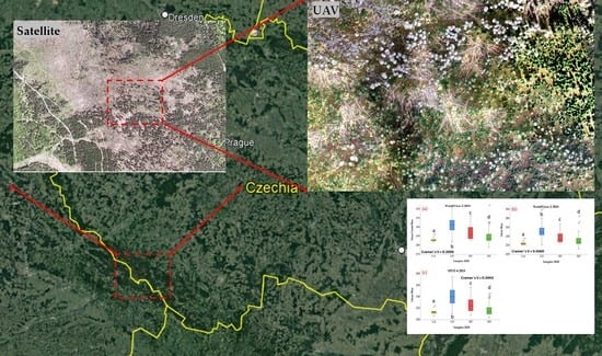
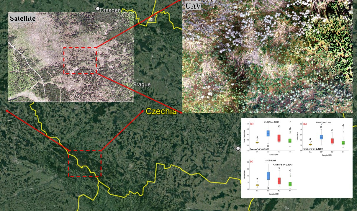
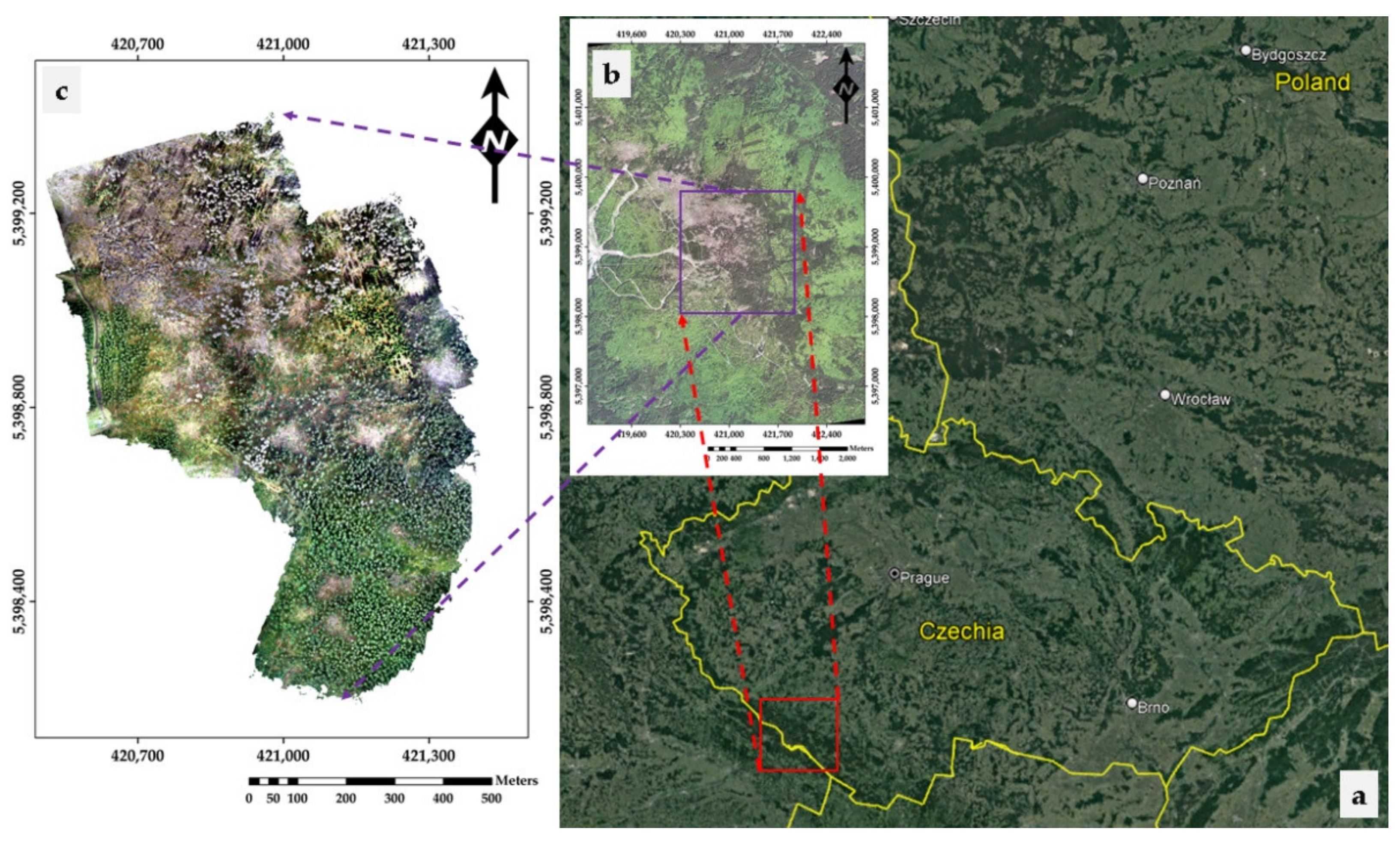
2.1. Study Area
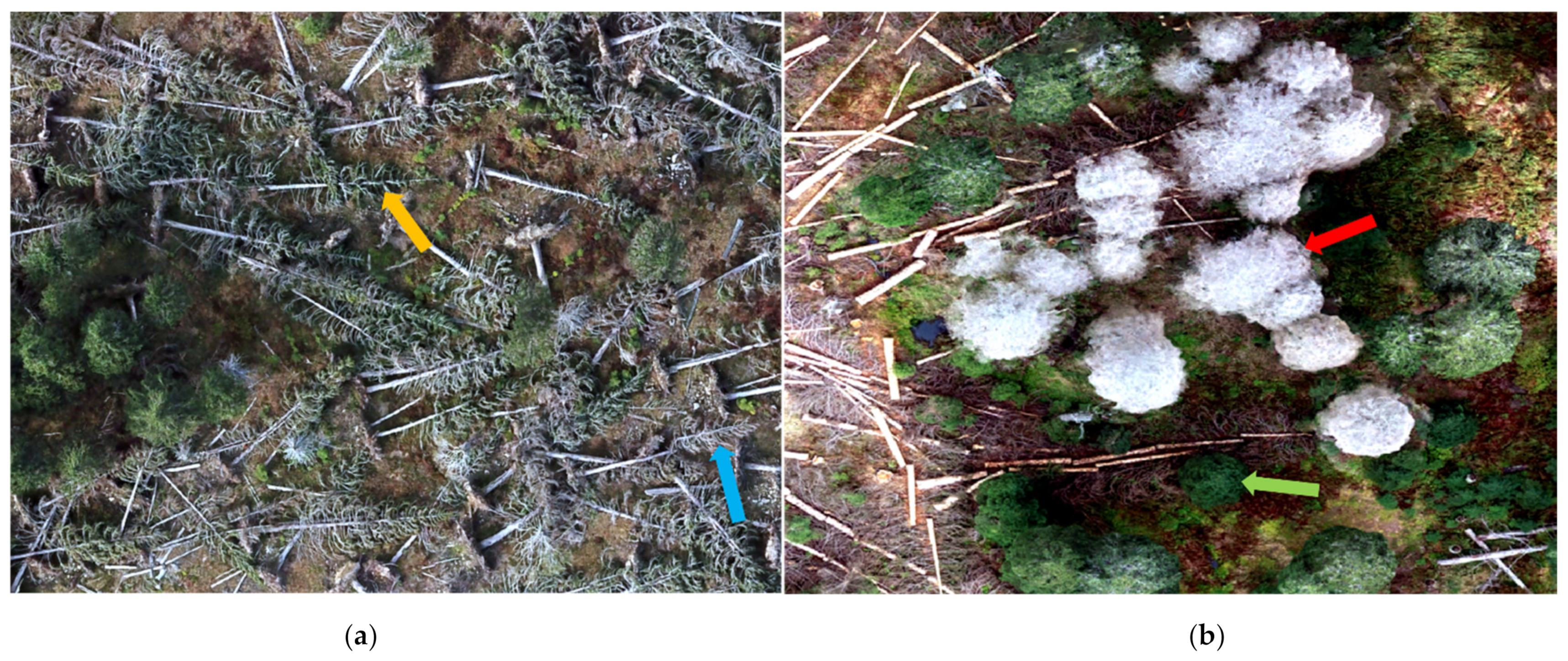
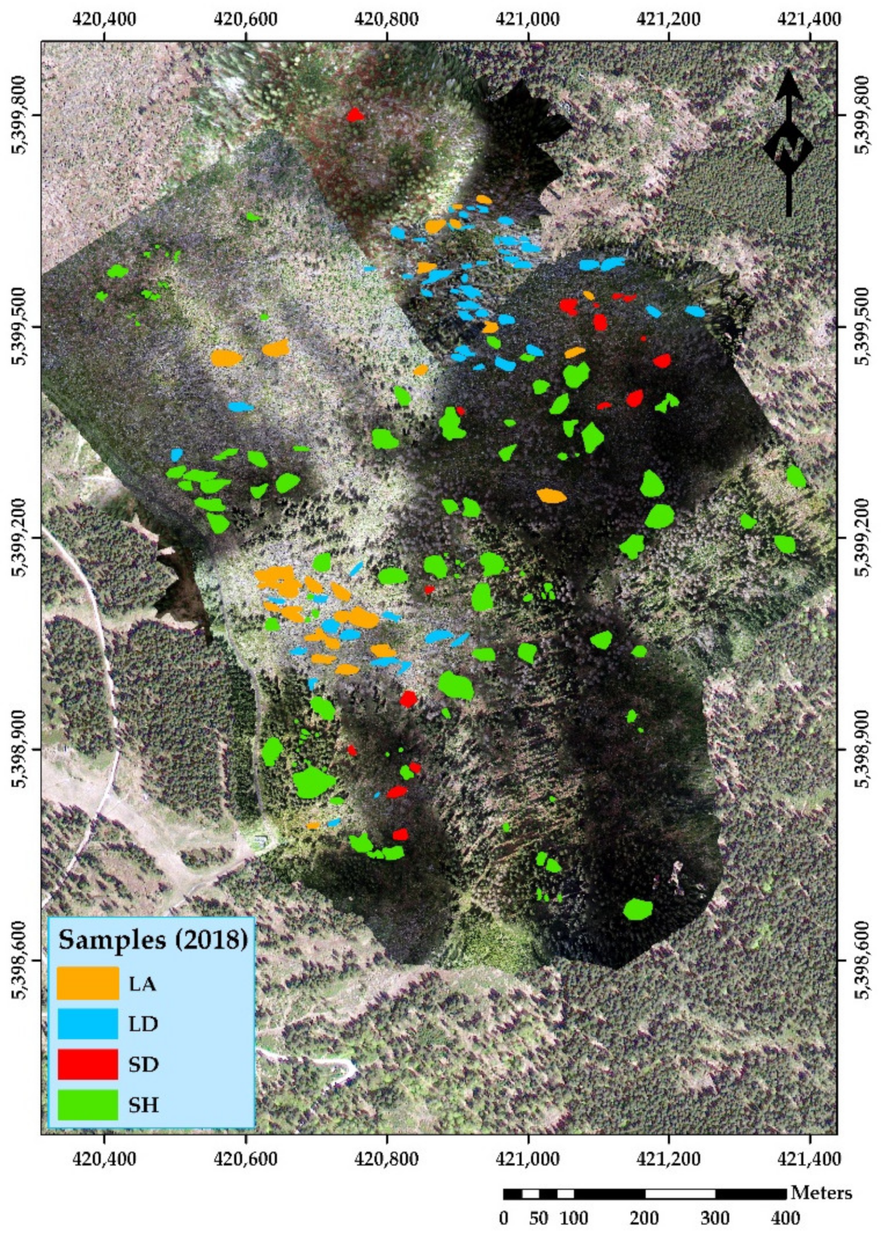
2.2. UAV Data Acquisition—Preprocessing and Sampling
2.3. Acquisition and Preprocessing of Satellite Imagery
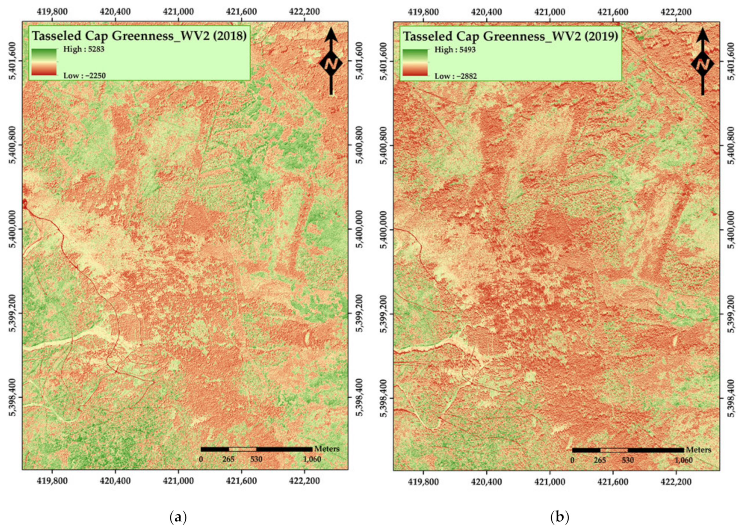
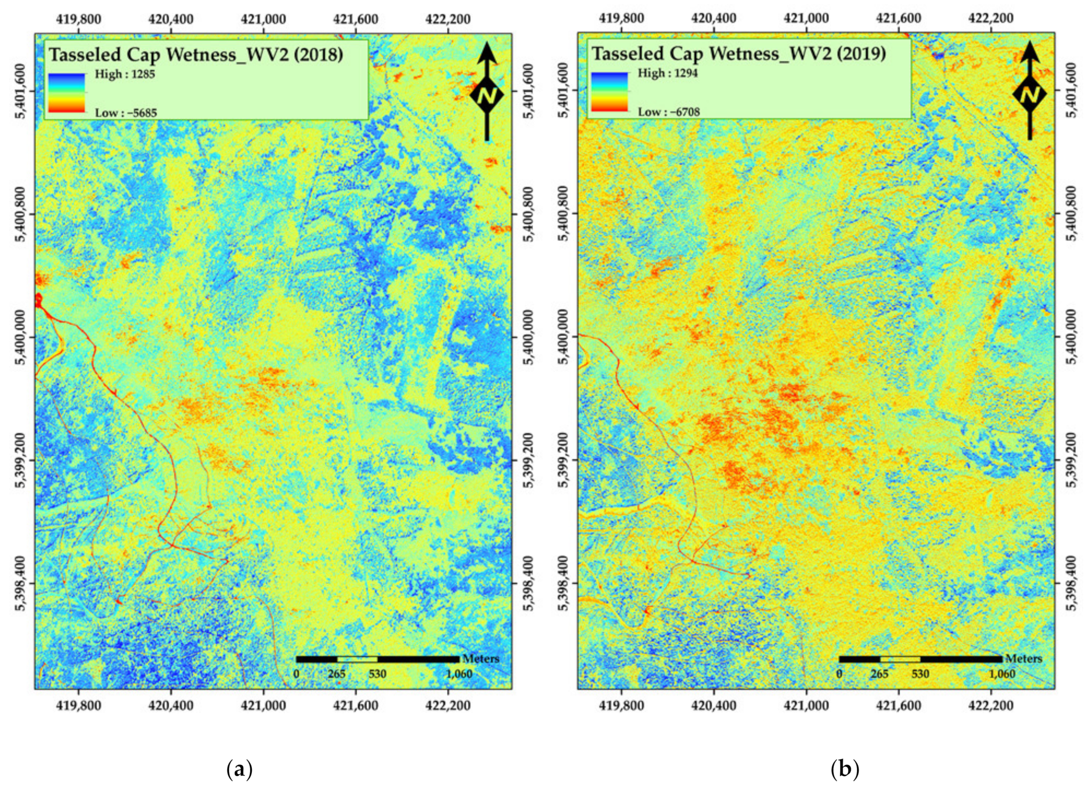
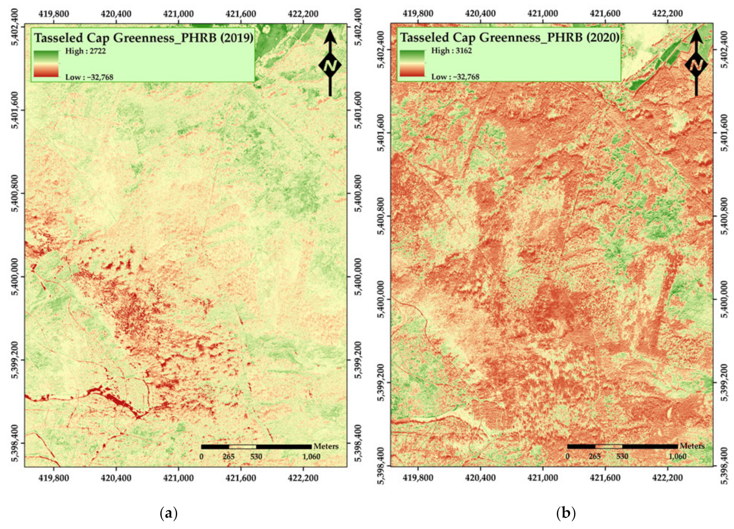
2.4. Processing of Spectral Satellite Data
2.5. Accuracy Assessment
3. Results
4. Discussion
5. Conclusions
Supplementary Materials
Author Contributions
Funding
Institutional Review Board Statement
Informed Consent Statement
Data Availability Statement
Acknowledgments
Conflicts of Interest
Appendix A


Appendix B


Appendix C


Appendix D


References
- Hlásny, T.; König, L.; Krokene, P.; Lindner, M.; Montagné-Huck, C.; Müller, J.; Qin, H.; Raffa, J.F.; Schelhaas, M.; Svoboda, M.; et al. Bark Beetle Outbreaks in Europe: State of Knowledge and Ways Forward for Management. Curr. For. Rep. 2021, 7, 138–165. [Google Scholar] [CrossRef]
- Grodzki, W. Mass outbreaks of the spruce bark beetle Ips typographus in the context of the controversies around the Białowieża Primeval Forest. For. Res. Pap. 2016, 77, 324–331. [Google Scholar] [CrossRef] [Green Version]
- Forest Management Institute of the Czech Republic. Information on the State of Forests from the Comprehensive Forest Management Plans for 2019. Available online: http://www.uhul.cz/ke-stazeni/informace-o-lese/slhp (accessed on 26 October 2020).
- Gardiner, B. Wind damage to forests and trees: A review with an emphasis on planted and managed forests. J. For. Res. 2021, 26, 248–266. [Google Scholar] [CrossRef]
- Bentz, B.J.; Jönsson, A.M.; Schroeder, M.; Weed, A.; Wilcke, R.A.I.; Larsson, K. Ips typographus and Dendroctonus ponderosae Models Project Thermal Suitability for Intra- and Inter-Continental Establishment in a Changing Climate. Front. For. Glob. Chang. 2019, 2, 1–17. [Google Scholar] [CrossRef]
- Marini, L.; Økland, B.; Jönsson, A.M.; Bentz, B.; Carroll, A.; Forster, B.; Grégoire, J.-C.; Hurling, R.; Nageleisen, L.M.; Netherer, S.; et al. Climate drivers of bark beetle outbreak dynamics in Norway spruce forests. Ecography 2017, 40, 1426–1435. [Google Scholar] [CrossRef]
- Brázdil, R.; Stucki, P.; Szabó, P.; Řezníčková, L.; Dolák, L.; Dobrovolný, P.; Tolasz, R.; Kotyza, O.; Chromá, K.; Suchánková, S. Windstorms and Forest Disturbances in the Czech Lands: 1801–2015. Agric. For. Meteorol. 2018, 250, 47–63. [Google Scholar] [CrossRef]
- Jakoby, O.; Lischke, H.; Wermelinger, B. Climate change alters elevational phenology patterns of the European spruce bark beetle (Ips typographus). Glob. Change Biol. 2019, 25, 4048–4063. [Google Scholar] [CrossRef]
- Modlinger, R.; Novotný, P. Quantification of time delay between damages caused by windstorms and by Ips typographus. For. J. 2015, 61, 221–231. [Google Scholar] [CrossRef] [Green Version]
- Hlásny, Τ.; Zimová, S.; Merganičová, K.; Štěpánek, P.; Modlinger, R.; Turčáni, M. Devastating outbreak of bark beeltes in the Czech Republic: Drivers, impacts and management implications. For. Ecol. Manag. 2021, 490, 119075. [Google Scholar] [CrossRef]
- Hlásny, T.; Merganičová, K.; Modlinger, R.; Marušák, R.; Löwe, R.; Turčáni, M. Prognosis of bark beetle outbreak and a new platform for the dissemination of information about the forests in the Czech republic. Rep. For. Res. 2021, 66, 197–205. [Google Scholar]
- Lausch, A.; Heurich, M.; Fahse, L. Spatio-Temporal Infestation Patterns of Ips Typographus (L.) in the Bavarian Forest National Park, Germany. Ecol. Indic. 2013, 31, 73–81. [Google Scholar] [CrossRef]
- Götz, L.; Psomas, A.; Bugmann, H. Early detection of bark beetle infestations by remote sensing: What is feasible today? Schweiz. Z. Forstwes. 2020, 171, 36–43. [Google Scholar] [CrossRef]
- Hall, R.J.; Castilla, G.; White, J.C.; Cooke, B.J.; Skakun, R.S. Remote sensing of forest pest damage: A review and lessons learned from a Canadian perspective. Can. Entomol. 2016, 148, S296–S356. [Google Scholar] [CrossRef]
- Hollaus, M.; Vreugdenhil, M. Radar Satellite Imagery for Detecting Bark Beetle Outbreaks in Forests. Curr. For. Rep. 2019, 5, 240–250. [Google Scholar] [CrossRef] [Green Version]
- Senf, C.; Seidl, R.; Hostert, P. Remote Sensing of Forest Insect Disturbances: Current State and Future Directions. Int. J. Appl. Earth Obs. Geoinf. 2017, 60, 49–60. [Google Scholar] [CrossRef] [Green Version]
- Lausch, A.; Erasmi, S.; King, D.J.; Magdon, P.; Heurich, M. Understanding forest health with remote sensing—Part I—A review of spectral traits, processes and remote-sensing characteristics. Remote Sens. 2016, 8, 1029. [Google Scholar] [CrossRef] [Green Version]
- Masek, J.G.; Hayes, D.J.; Hughes, J.M.; Healey, S.P.; Turner, D.P. The role of remote sensing in process-scaling studies of managed forest ecosystems. For. Ecol. Manag. 2015, 355, 109–123. [Google Scholar] [CrossRef] [Green Version]
- Abdollahnejad, A.; Panagiotidis, D.; Bílek, L. An Integrated GIS and Remote Sensing Approach for Monitoring Harvested Areas from Very High-Resolution, Low-Cost Satellite Images. Remote Sens. 2019, 11, 2539. [Google Scholar] [CrossRef] [Green Version]
- Abdollahnejad, A.; Panagiotidis, D.; Surový, P. Estimation and Extrapolation of Tree Parameters Using Spectral Correlation between UAV and Pléiades Data. Forests 2018, 9, 85. [Google Scholar] [CrossRef] [Green Version]
- Wagner, F.H.; Ferreira, M.P.; Sanchez, A.; Hirye, M.C.M.; Gloor, M.Z.E.; Philips, O.L.; de Souza Filho, C.R.; Shimabukuro, Y.E.; Aragao, L.E.O.C. Individual tree crown delineation in a highly diverse tropical forest using very high-resolution satellite images. ISPRS J. Photogramm. Remote Sens. 2018, 145, 362–377. [Google Scholar] [CrossRef]
- Eitel, J.U.H.; Vierling, L.A.; Litvak, M.E.; Long, D.S.; Schulthess, U.; Ager, A.A.; Krofcheck, D.J.; Stosheck, L. Broadband, red-edge information from satellites improves early stress detection in a New Mexico conifer woodland. Remote Sens. Environ. 2001, 115, 3640–3646. [Google Scholar] [CrossRef]
- Fassnacht, F.E.; Latifi, H.; Ghosh, A.; Joshi, P.K.; Koch, B. Assessing the potential of hyperspectral imagery to map bark beetle-induced tree mortality. Remote Sens. Environ. 2014, 140, 533–548. [Google Scholar] [CrossRef]
- Adamczyk, J.; Osberger, A. Red-edge vegetation indices for detecting and assessing disturbances in Norway spruce dominated mountain forests. Int. J. Appl. Earth Obs. Geoinf. 2015, 37, 90–99. [Google Scholar] [CrossRef]
- Immitzer, M.; Atzberger, C. Early Detection of Bark Beetle Infestation in Norway Spruce (Picea abies, L.) using WorldView-2 Data. Photogramm. Fernerkund. Geoinf. 2014, 5, 0351–0367. [Google Scholar] [CrossRef]
- Mullen, K.E. Early Detection of Mountain Pine Beetle Damage in Ponderosa Pine Forests of the Black Hills Using Hyperspectral and WorldView-2 Data. Master’s Thesis, Minnesota State University, Mankato, MN, USA, 2016. [Google Scholar]
- Filchev, L. An assessment of European spruce bark beetle infestation using WorldView-2 Satellite data. In Proceedings of the 1st European SCGIS Conference with International Participation―Best Practices: Application of GIS Technologies for Conservation of Natural and Cultural Heritage Sites, Sofia, Bulgaria, 21–23 May 2012; SRTI-Bulgarian Academy of Science (BAS) and SCGIS: Sofia, Bulgaria, 2010. [Google Scholar]
- Huo, L.; Persson, H.J.; Lindberg, E. Early detection of forest stress from European spruce bark beetle attack, and a new vegetation index: Normalized distance red & SWRIR (NDRS). Remote Sens. Environ. 2021, 255, 112240. [Google Scholar]
- Lukeš, P.; Strejček, R.; Křístek, Š.; Mlčoušek, M. Forest Health Assessment in Czech Republic Using Sentinel-2 Satellite Data. Certified Methodology; Forest Management Institute: Brandýs nad Labem, Czech Republic, 2018; ISBN 978-80-88184-21-8. [Google Scholar]
- Barka, I.; Lukeš, P.; Bucha, T.; Hlásny, T.; Strejček, R.; Mlčoušek, M.; Křístek, Š. Remote sensing-based forest health monitoring systems—Case studies from Czechia and Slovakia. Cent. Eur. For. J. 2018, 64, 259–275. [Google Scholar]
- Albrecht, J. Českobudějovicko. In Chráněná Území ČR, Svazek VIII.; Mackovčin, P., Sedláček, M., Eds.; AOPK ČR a EkoCentrum: Brno, Praha, Czech Republic, 2003; p. 808. [Google Scholar]
- Hotelling, H. Analysis of a complex of statistical variables into principal components. J. Educ. Psychol. 1933, 24, 498–520. [Google Scholar] [CrossRef]
- Crist, E.P.; Cicone, R.C. Application of the tasseled cap concept to simulated thematic mapper data. Photogramm. Eng. Remote Sens. 1984, 50, 343–352. [Google Scholar]
- Crist, E.P.; Cicone, R.C. A physically-based transformation of thematic mapper data—The TM tasseled cap. IEEE Trans. Geosci. Remote Sens. 1984, GE-22, 256–263. [Google Scholar] [CrossRef]
- Horne, J.H. A tasseled cap transformation for Ikonos images. In Proceedings of the ASPRS 2003 Annual Conference Proceedings, Anchorage, AK, USA, 3–9 May 2003; pp. 1–7. [Google Scholar]
- Huang, C.; Wylie, B.; Yang, L.; Homer, C.; Zylstra, G. Derivation of a tasseled cap transformation based on Landsat 7 at-satellite reflectance. Int. J. Remote Sens. 2002, 23, 1741–1748. [Google Scholar] [CrossRef]
- Ivits, E.; Lamb, A.; Langar, F.; Hemphill, S.; Koch, B. Orthogonal transformation of segmented SPOT5 images. Photogramm. Eng. Remote Sens. 2008, 74, 1351–1364. [Google Scholar] [CrossRef]
- Huete, A. A soil-adjusted vegetation index (SAVI). Remote Sens. Environ. 1988, 25, 295–309. [Google Scholar] [CrossRef]
- Rouse, J.; Haas, J.W.J.; Schell, R.H.; Deering, J.A. Monitoring vegetation systems in the great plains with ERTS. In Proceedings of the Third ERTS Symposium (NASA SP-351), Washington, DC, USA, 1 January 1974; pp. 309–317. [Google Scholar]
- Birth, G.S.; McVey, G.R. Measuring the Color of Growing Turf with a Reflectance Spectrophotometer 1. Agron. J. 1968, 60, 640–643. [Google Scholar] [CrossRef]
- Deering, D.W.; Rouse, J.W.; Haas, R.H.; Schell, J.A. Measuring Forage Production of Grazing Units from Landsat MSS Data. In Proceedings of the 10th International Symposium on Remote Sensing of Environment, Ann Arbor, MI, USA, 6–10 October 1975; pp. 1169–1178. [Google Scholar]
- Daughtry, C.S.T. Estimating Corn Leaf Chlorophyll Concentration from Leaf and Canopy Reflectance. Remote Sens. Environ. 2000, 74, 229–239. [Google Scholar] [CrossRef]
- Ren, S.; Chen, X.; An, S. Assessing plant senescence reflectance index-retrieved vegetation phenology and its spatiotemporal response to climate change in the Inner Mongolian Grassland. Int. J. Biometeorol. 2016, 61, 601–612. [Google Scholar] [CrossRef] [PubMed]
- Clarke, T.; Moran, M.; Barnes, E.; Pinter, P.; Qi, J. Planar domain indices: A method for measuring a quality of a single component in two-component pixels. In Proceedings of the IGARSS 2001. Scanning the Present and Resolving the Future. In Proceedings of the IEEE 2001 International Geoscience and Remote Sensing Symposium (Cat. No.01CH37217), Sydney, NSW, Australia, 9–13 July 2001; pp. 1279–1281. [Google Scholar]
- Abdollahnejad, A.; Panagiotidis, D. Tree Species Classification and Health Status Assessment for a Mixed Broadleaf-Conifer Forest with UAS Multispectral Imaging. Remote Sens. 2020, 12, 3722. [Google Scholar] [CrossRef]
- Matsuki, T.; Yokoya, N.; Iwasaki, A. Hyperspectral Tree Species Classification of Japanese Complex Mixed Forest with the Aid of Lidar Data. IEEE J. Sel. Top. Appl. Earth Obs. Remote Sens. 2015, 8, 2177–2187. [Google Scholar] [CrossRef]
- Gilewski, M. The role of light in the plants world. Photonics Lett. Pol. 2019, 11, 115–117. [Google Scholar] [CrossRef]
- Huggett, B.A.; Savage, J.A.; Hao, G.-Y.; Preisser, E.L.; Holbrook, N.M. Impact of hemlock woolly adelgid (Adelges tsugae) infestation on xylem structure and function and leaf physiology in eastern hemlock (Tsuga canadensis). Funct. Plant Biol. 2017, 45, 501–508. [Google Scholar] [CrossRef]
- Ford, M.C.; Zietlow, D.R.; Brantley, S.T.; Brown, C.L.; Albert, M.E., III.; Jetton, R.M.; Rhea, J.R.; Arnold, P. Physiological responses of eastern hemlock (Tsuga canadensis) to light, adelgid infestation, and biological control: Implications for hemlock restoration. For. Ecol. Manag. 2020, 460, 117903. [Google Scholar]
- Jones, H.G.; Vaughan, R.A. Remote Sensing of Vegetation: Principles, Techniques, and Applications; Oxford University Press: Oxford, UK, 2010; Volume 68. [Google Scholar]
- Ollinger, S.V. Sources of variability in canopy reflectance and the convergent properties of plants. New Phytol. 2010, 189, 375–394. [Google Scholar] [CrossRef]
- Lillesand, T.; Kiefer, R.W.; Chipman, J. Remote Sensing and Image Interpretation; John Wiley and Sons: Hoboken, NJ, USA, 2015. [Google Scholar]
- Guerra-Hernández, J.; Díaz-Varela, R.A.; Ávarez-González, J.G.; Rodríguez-González, P.M. Assessing a novel modelling approach with high resolution UAV imagery for monitoring health status in priority riparian forests. For. Ecosyst. 2021, 8, 61. [Google Scholar] [CrossRef]
- Liu, Q.; Liu, G. Using Tasseled Cap Transformation of CBERS-02 Images to Detect Dieback or Dead Robinia pseudoacacia Plantation. In Proceedings of the IEEE 2009 2nd International Congress on Image and Signal Processing, Tianjin, China, 17–19 October 2009; 2009; pp. 1–5. [Google Scholar] [CrossRef]
- Erener, A. Remote sensing of vegetation health for reclaimed areas of Seyitömer open cast coal mine. Int. J. Coal. Geol. 2011, 86, 20–26. [Google Scholar] [CrossRef]


| Year | Classes | Sample Frequency | Average Area (m2) | Sum of Area (m2) |
|---|---|---|---|---|
| 2018 | 1 LA | 30 | 218.62 | 6558.69 |
| 1 LD | 55 | 164.68 | 9057.24 | |
| 1 SD | 18 | 185.67 | 3342.04 | |
| 1 SH | 109 | 284.23 | 30,981.56 | |
| 2019 | 1 LA | 21 | 228.74 | 4803.56 |
| 1 LD | 66 | 171.21 | 11,299.85 | |
| 1 SD | 19 | 168.38 | 3199.16 | |
| 1 SH | 106 | 289.03 | 30,636.98 | |
| 2020 | 1 LA | 10 | 349.22 | 3492.23 |
| 1 LD | 89 | 185.08 | 16,471.75 | |
| 1 SD | 45 | 350.71 | 15,781.75 | |
| 1 SH | 68 | 208.73 | 14,193.81 |
| Satellite Platform | Imagery Products Resolution | Spectral Bands (nm) | Image Location Accuracy |
|---|---|---|---|
| Pléiades 1B | 2 m multispectral—0.50 m PAN | Red: 600–720 | With 1 GPSs is 1 m; without GPSs is 3 m (CE90) |
| Green: 490–610 | |||
| Blue: 430–550 | |||
| NIR: 750–950 | |||
| PAN: 480–830 | |||
| WorldView-2 | 1.64 m multispectral—0.41 m PAN | Coastal blue: 400–450 | ≤3 m (using a GPS receiver, a gyroscope, and a star tracker) without any GCPs |
| Blue: 450–510 | |||
| Green: 510–580 | |||
| Yellow: 585–625 | |||
| Red: 630–690 | |||
| Red edge: 705–745 | |||
| NIR1: 770–895 | |||
| NIR2: 860–1040 | |||
| PAN: 450–800 | |||
| SPOT-6 | 6 m multispectral—1.5 m PAN | Red: 620–690 | 35 m CE 90 without GCP within 30 viewing angle cone; 10 m CE90 for Ortho where Reference3D is available |
| Blue: 450–520 | |||
| Green: 530–600 | |||
| NIR: 760–890 | |||
| PAN: 450–750 |
| Satellite Platform | Used Indices | Formula | Citation |
|---|---|---|---|
| Pléiades 1B SPOT-6 | Soil Adjusted Vegetation Index (SAVI) | [1.5 × (NIR − Red)]/(NIR + Red + 0.5) | Huete [38] |
| Normalized Difference Vegetation Index (NDVI) | (NIR − Red/NIR + Red) | Rouse et al. [39] | |
| Simple Ratio (SR) | (NIR/Red) | Birth and McVey [40] | |
| Transformed Vegetation Index (TVI) | 1 SQRT((NIR − Red)/(NIR + Red) + 0.5) | Deering et al. [41] | |
| WorldView-2 | Soil Adjusted Vegetation Index (SAVI) | [1.5 × (NIR − Red)]/(NIR + Red + 0.5) | Huete [38] |
| Normalized Difference Vegetation Index (NDVI) | (NIR − Red/NIR + Red) | Rouse et al. [39] | |
| Simple Ratio (SR) | (NIR/Red) | Birth and McVey [40] | |
| Transformed Vegetation Index (TVI) | SQRT((NIR − Red)/(NIR + Red) + 0.5) | Deering et al. [41] | |
| Modified Chlorophyll Absorption Ratio Index (MCARI) | [(Red-edge − Red) − 0.2 × (Red-edge − Green)] × (Red-edge/Red) | Daughtry et al. [42] | |
| Plant Senescence Reflectance Index (PSRI) | (Red − Green)/(Red-edge) | Ren et al. [43] | |
| Normalized Difference Red-edge Index (NDRE) | (NIR − Red-edge)/(NIR + Red-edge) | Clarke et al. [44] |
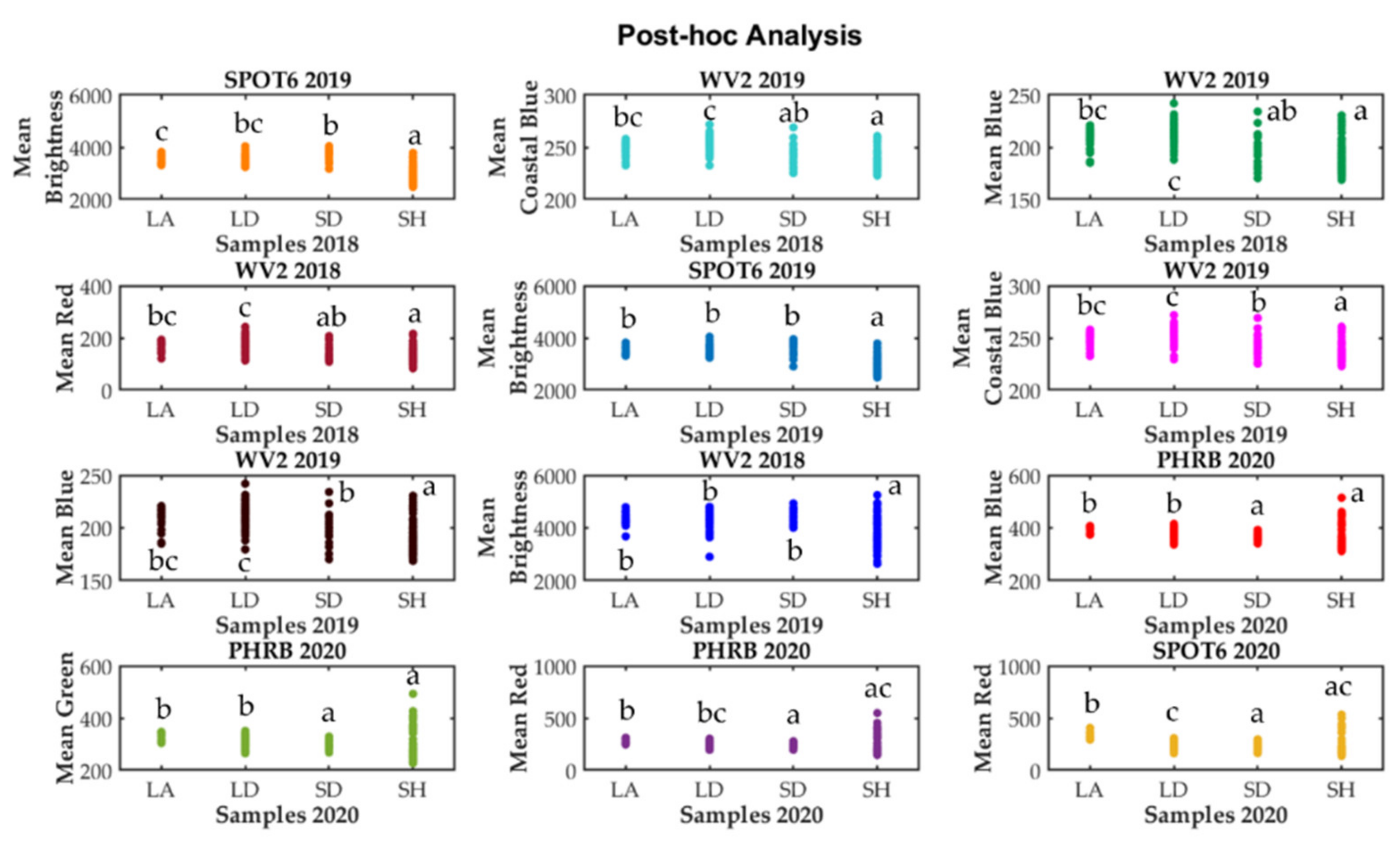
| Satellite | Year of Imagery | Band | ETA-Squared (2018) | ETA-Squared (2019) | ETA-Squared (2020) |
|---|---|---|---|---|---|
| PHRB | 2019 | NDVI (mean) | 0.34 | 0.33 | 0.28 |
| SAVI (mean) | 0.34 | 0.33 | 0.28 | ||
| SR (mean) | 0.38 | 0.38 | 0.34 | ||
| TVI (mean) | 0.33 | 0.32 | 0.27 | ||
| Wetness (mean) | 0.21 | 0.18 | 0.15 | ||
| 2020 | Greenness (mean) | 0.12 | 0.14 | 0.04 |
| Satellite | Year of Imagery | Band | ETA-Squared (2018) | ETA-Squared (2019) | ETA-Squared (2020) |
|---|---|---|---|---|---|
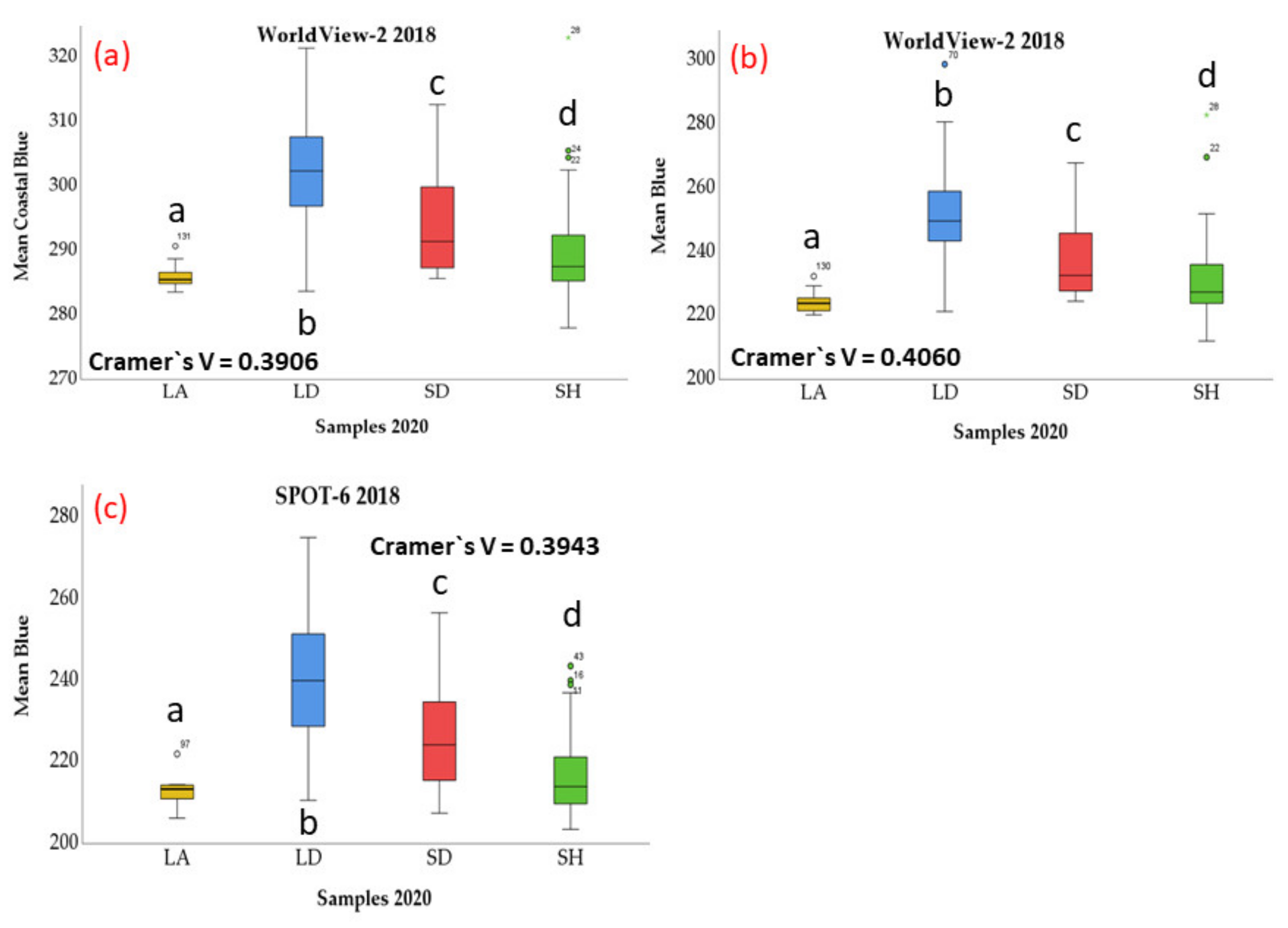
| WV2 | 2018 | Coastal Blue (mean) | 0.37 | 0.36 | 0.36 |
| Blue (mean) | 0.36 | 0.34 | 0.35 | ||
| Green (mean) | 0.33 | 0.31 | 0.32 | ||
| Yellow (mean) | 0.42 | 0.40 | 0.40 | ||
| Red (mean) | 0.41 | 0.39 | 0.40 | ||
| Brightness (mean) | 0.36 | 0.38 | 0.28 | ||
| Wetness (min) | 0.30 | 0.30 | 0.36 | ||
| 2019 | Coastal Blue (mean) | 0.52 | 0.49 | 0.58 | |
| Blue (mean) | 0.51 | 0.48 | 0.57 | ||
| Green (mean) | 0.45 | 0.43 | 0.49 | ||
| Yellow (mean) | 0.46 | 0.44 | 0.54 | ||
| Red (mean) | 0.48 | 0.46 | 0.60 | ||
| PSRI | 0.25 | 0.24 | 0.29 | ||
| Wetness (min) | 0.34 | 0.33 | 0.51 |
| Satellite | Year of Imagery | Band | ETA-Squared (2018) | ETA-Squared (2019) | ETA-Squared (2020) |
|---|---|---|---|---|---|
| SPOT6 | 2018 | Blue (mean) | 0.40 | 0.38 | 0.39 |
| Green (mean) | 0.38 | 0.37 | 0.39 | ||
| Red (mean) | 0.41 | 0.40 | 0.41 | ||
| Brightness (mean) | 0.36 | 0.36 | 0.28 | ||
| Wetness (mean) | 0.40 | 0.38 | 0.43 | ||
| SR (mean) | 0.21 | 0.21 | 0.26 | ||
| 2019 | Blue (mean) | 0.40 | 0.38 | 0.49 | |
| Green (mean) | 0.41 | 0.40 | 0.43 | ||
| Red (mean) | 0.38 | 0.36 | 0.46 | ||
| Brightness (mean) | 0.58 | 0.58 | 0.42 | ||
| Greenness(mean) | 0.27 | 0.22 | 0.04 | ||
| Wetness (median) | 0.27 | 0.21 | 0.12 | ||
| 2020 | Blue (min) | 0.19 | 0.18 | 0.26 | |
| Green (min) | 0.15 | 0.14 | 0.19 |
Publisher’s Note: MDPI stays neutral with regard to jurisdictional claims in published maps and institutional affiliations. |
© 2021 by the authors. Licensee MDPI, Basel, Switzerland. This article is an open access article distributed under the terms and conditions of the Creative Commons Attribution (CC BY) license (https://creativecommons.org/licenses/by/4.0/).
Share and Cite
Abdollahnejad, A.; Panagiotidis, D.; Surový, P.; Modlinger, R. Investigating the Correlation between Multisource Remote Sensing Data for Predicting Potential Spread of Ips typographus L. Spots in Healthy Trees. Remote Sens. 2021, 13, 4953. https://0-doi-org.brum.beds.ac.uk/10.3390/rs13234953
Abdollahnejad A, Panagiotidis D, Surový P, Modlinger R. Investigating the Correlation between Multisource Remote Sensing Data for Predicting Potential Spread of Ips typographus L. Spots in Healthy Trees. Remote Sensing. 2021; 13(23):4953. https://0-doi-org.brum.beds.ac.uk/10.3390/rs13234953
Chicago/Turabian StyleAbdollahnejad, Azadeh, Dimitrios Panagiotidis, Peter Surový, and Roman Modlinger. 2021. "Investigating the Correlation between Multisource Remote Sensing Data for Predicting Potential Spread of Ips typographus L. Spots in Healthy Trees" Remote Sensing 13, no. 23: 4953. https://0-doi-org.brum.beds.ac.uk/10.3390/rs13234953