Article

Quantifying Crown Morphology of Mixed Pine-Oak Forests Using Terrestrial Laser Scanning

1
Instituto Universitario de Investigación y Gestión Forestal Sostenible—iuFOR, Universidad de Valladolid—INIA, Avda. Madrid s/n, 34004 Palencia, Spain
2
Departamento de Produccion Vegetal y Recursos Forestales, Campus de Palencia—Universidad de Valladolid, 34004 Palencia, Spain
3
Department of Forest Resources Management, Faculty of Forestry, The University of British Columbia, 2424 Main Mall, Vancouver, BC V6T 1Z4, Canada
4
Departamento Estadística e Investigación Operativa, Campus de Palencia—Universidad de Valladolid, 34004 Palencia, Spain
5
Department of Silviculture and Forest Ecology of the Temperate Zones, Faculty of Forest Science, University of Göttingen, Büsgenweg 1, 37077 Göttingen, Germany
6
Department for Spatial Structures and Digitization of Forests, Faculty of Forest Science, University of Göttingen, Büsgenweg 1, 37077 Göttingen, Germany
*
Author to whom correspondence should be addressed.
Remote Sens. 2021, 13(23), 4955; https://0-doi-org.brum.beds.ac.uk/10.3390/rs13234955
Submission received: 8 October 2021 / Revised: 14 November 2021 / Accepted: 16 November 2021 / Published: 6 December 2021
(This article belongs to the Special Issue Terrestrial Laser Scanning of Forest Structure)

Abstract

:
Mixed forests make up the majority of natural forests, and they are conducive to improving the resilience and resistance of forest ecosystems. Moreover, it is in the crown of the trees where the effect of inter- and intra-specific interaction between them is evident. However, our knowledge of changes in crown morphology caused by density, competition, and mixture of specific species is still limited. Here, we provide insight on stand structural complexity based on the study of four response crown variables (Maximum Crown Width Height, MCWH; Crown Base Height, CBH; Crown Volume, CV; and Crown Projection Area, CPA) derived from multiple terrestrial laser scans. Data were obtained from six permanent plots in Northern Spain comprising of two widespread species across Europe; Scots pine (Pinus sylvestris L.) and sessile oak (Quercus petraea (Matt.) Liebl.). A total of 193 pines and 256 oaks were extracted from the point cloud. Correlation test were conducted (ρ ≥ 0.9) and finally eleven independent variables for each target tree were calculated and categorized into size, density, competition and mixture, which was included as a continuous variable. Linear and non-linear multiple regressions were used to fit models to the four crown variables and the best models were selected according to the lowest AIC Index and biological sense. Our results provide evidence for species plasticity to diverse neighborhoods and show complementarity between pines and oaks in mixtures, where pines have higher MCWH and CBH than oaks but lower CV and CPA, contrary to oaks. The species complementarity in crown variables confirm that mixtures can be used to increase above ground structural diversity.

Graphical Abstract

1. Introduction

Trees determine the living conditions for many other organism groups and, typically, they are the most valuable economical component for forests. Therefore, the tree layer is often the compartment of forest ecosystems that is most strongly modified by humans through their management activity [1]. In this regard, much knowledge exists concerning monocultures, which have been largely studied by the scientific community, even though natural forests are typically mixed forests [1] where species’ interaction creates more complex forest structures (which make it harder for their dynamics to be understood). A mixed forest is defined as a forest unit of at least 0.5 ha that is composed of no less than two tree species at any developmental stage, sharing common resources as water, light and, soil nutrients [2].
Trees of the same species grow differently in monocultures and mixtures [3] and empirical evidence suggests that species mixing can improve resource utilization within stands [4] due to the complementarity effect, which could be either due to reduced competition or increased facilitation [5]. Tree species with different growth rates and final heights will likely develop structurally more diverse forests than those composed of only one or few species [3] creating multilayered canopies that absorb more light [6]. An increase in tree species diversity can generate a variety of forest structures and interaction between the component species [7], which may lead to more resistant, resilient, and adaptable forests [2,3], and therefore, an important risk-reduction strategy [8]. For this reason, within the last two decades, to understand and manage species’ behavior in mixed conditions, many researchers have focused on the performance of mixed forests species input [2,9,10]. Several studies have already shown that mixed stands may have more biomass production than their respective pure stands [8,9,10,11] compared to monocultures [12,13]. Few have studied the mechanisms underlying the mixing effect on productivity [5,10] and confirmed higher rates of primary production in complex forest structures [6]. However, the understanding of tree species interaction in their structure and functioning is still poor [14]. Considering that mixed forests dynamics vary on a small scale [15] more studies are still needed across a variety of forest types to establish a sound theoretical approach across scales.
To understand forest dynamics, Diameter at Breast Height (DBH) and Total Tree Height (TH) are the two most common and easy variables for measuring, analyzing, and modeling forest stands [16]. They are used separately or together in addition with tree species for estimating other important single-tree attributes such as the stem volume, biomass, or the crown [17]. However, it is important to have an accurate measure and knowledge of the crowns because the crown of a tree accomplishes multiple functions [18] and is very heterogeneous in shape despite similar overall tree dimensions [15]. In a stand, crowns are where the effect of inter and intra-specific interaction between trees have been shown [18,19,20]. The crown might allow the trees within a stand to fully utilize limited resources in different spaces and times compared to a monoculture of any species [2]. The tree crown allometry proved to be essential for understanding, appropriate modelling, and silvicultural regulation of mixed stands. For this reason, continuous allometric analyses of various kinds of tree species mixtures need to be done [21].
Historically, the crown has been measured indirectly through empirical established relationships with conventional approaches (mean diameter, dominant height, or volume per hectare), which are relatively easy to make, repeatable, and transferrable. However, they are laborious and imprecise with conventional methods [15] and lead to some problems. For example, they are difficult to validate, difficult to generalize, and uncertainties are poorly quantified or even unknown [22]. In addition, they ignore the three-dimensional nature of stand structure, its most important characteristic (Pretzsch, 2009) basing the results on geometric standard crown shapes [15]. The structural complexity increases in mixed forests due to the different growth rates of each species [23], and other processes resulting in spatial niche-partitioning [24] simplified crown forms are not valid anymore to represent the heterogeneity of this kind of forests [15], and more efficient algorithms need to be developed to calculate tree crown variables to facilitate a complete forest resource survey [18]. To overcome these issues, Terrestrial Laser Scanning (TLS) has shown to hold great potential [25]. TLS enables us to quantify the effect of mixed forest in stand dynamics, e.g., [19,26,27,28,29,30,31,32]. Species identity modifies the mixture outcomes [2], for that reason all possible species mixtures need to be assessed, thus, an adequate management strategy for each species composition can be defined [2].
Within the last decade understanding and predicting influences of inter-specific competition is becoming increasingly important due to an emphasis on mixed-species management [33]. Most studies on mixed-species dynamics were focused on Pinus sylvestris, the species with the biggest area extension in Europe [34,35], together with other central European species like Picia abies or Fagus sylvatica e.g., [29,31,36,37,38,39]. And few studies were focused on the interaction pine-oak using conventional methods [4,40,41]. Quercus petraea together with Quercus robur, are the two most widespread oak species in Central Europe [42], and are considered helpful for creating more climate-resilient mixed stands thanks to their broad ecological amplitude [42]. In addition, Quercus petraea has a very high environmental and protector value as montane species which, makes it necessary to consider its conservation [43,44,45].
The purpose of this study was to gain a deeper and more accurate insight into the interaction between these two important and widespread species in Europe, Sessile Oak (Quercus petraea) and Scots Pine, (Pinus sylvestris) [46] by analyzing their crown variables through the use of TLS. The basic parameter to define the crown of a tree, according to Lin et al. [18] are crown height, crown volume, and crown projection. In this study, we have analyzed the crown variables Crown Base Height (CBH) and the Maximum Crown Width Height (MCWH) also known as Height of Maximum Crown Extension but MCWH will be used throughout this paper, and as crown size variables the Crown Projection Area (CPA), and the Crown Volume (CV). Analyzing these crown variables, we want to address and determine how the intra and inter-specific competition affects the crown shape of these two species. For this purpose, six pine-oak mixed stands were scanned, and we determined the following research questions:
(1)
Have pines and oaks different Diameter Breast Height (DBH) and Total Height of the tree (HT) growing in pure vs. mixed stands?
(2)
Have the explanatory variables of size, density, competition, and mixture a positive or negative relationship in their crown variables (Response variables)?

2. Material and Method

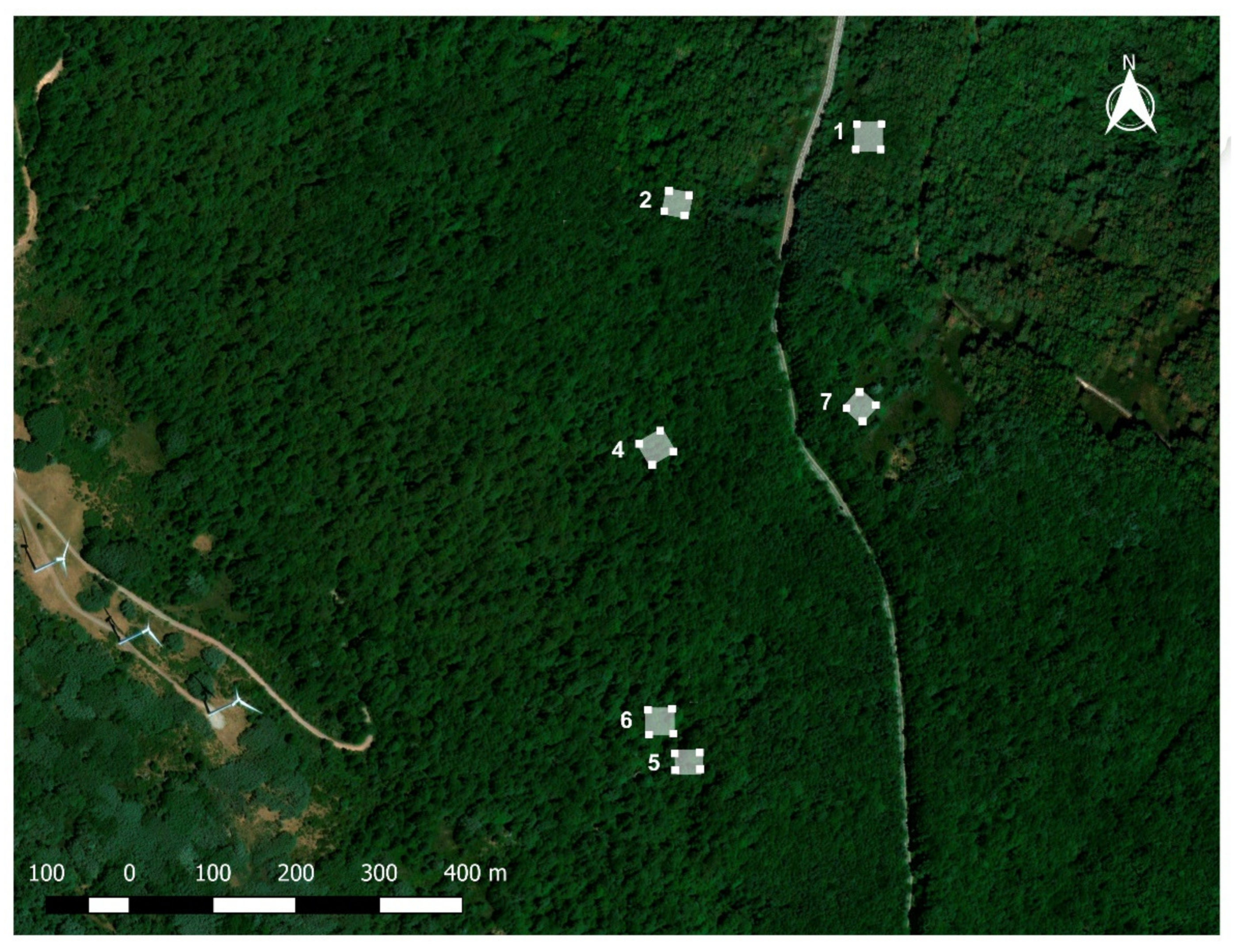
2.1. Study Area and Experimental Setup

Our study was based on a Pinus silvestrys and Quercus petraea forest located in the region of Castilla y Leon in Northern Spain (42°54′48″ N, 4°14′31″ W, which is a neigh-boring region between continental and Atlantic climate. The area is thus characterized by both continental and Atlantic influences in the climate (mean annual temperature of 9.9 °C and a mean annual precipitation 1044 mm). Pines were planted at the beginning of the ‘70s, and oaks have naturally regrown and no thinning was done in this area in the last 10 years. In 2017, to gain insight into the forest growth dynamic of these two European species in mixed conditions compared to pure conditions, two triplets were established. Each triplet consists of three plots. All plots are located next to each other and have similar site conditions (Figure 1). The Permanent plots set within each triplet are rectangular, limits are marked with wooden poles 50 cm height in each corner. Plots sizes varied to include at least 40 trees of each species of which at least 20 in total are dominant (Table 1). In the pure pine stands the proportion of pine stems varies from 73.1% to 90%, and in pure oak stands from 85.3% to 95.3%. Finally, in the mixed stands, pines and oaks vary from 41.1% to 45.7%, and from 52.4% to 58.9% respectively. From here, data were collected, and analyzed as shown in the work diagram (Figure 2).

2.2. Field Data Collection

2.2.1. Conventional Measurements

For each tree with a Diameter at Breast Height (DBH) above 7 cm, species were identified, labeled (tree ID) and its position (Cartesian x and y coordinates) recorded with a Total Station Topcon 220. DBH was measured with a caliper (cm); total height and height to crown base were measured in m with Vertex III (Haglöf, Sweden). Finally, tree crown projection radii (in four directions: N, E, S, W) were measured with tape to the closest cm. Table 2 summarizes the stand characteristics for each species.

2.2.2. Terrestrial Laser Scanning

Terrestrial laser scanning (TLS) data were acquired in February and March 2020. Prior to scanning, we georeferenced the plots with a sub-metric GPS Leica model SR20 single frequency equipment with external antenna reception AT501. We recorded 3 corners of each plot for at least 30 min to minimize errors. Each of the points was identified in the field to be easily recognizable through the scanner images. This way, we could overlap point clouds with the map of trees created by the total station Topcon 220 to identify each tree measured with our point cloud files.
TLS data were captured using a Faro Focus 3D device. The laser scanner was mounted on a tripod at approximately 1.3 m above the ground. The settings characteristics are shown in Table 3. To cover all trees belonging to the plots, a pre-design of multiple-scan approach on each tree-plot map with approximately 12 scanner positions per plot was performed. However, the final amount of scanner positions varied depending on stand density to reduce obstruction and assure that tree stems were captured from all sides. To co-register the scans from all the different perspectives to one single point cloud, 15 white plastic spheres 18 cm in diameter placed on one-meter wooden poles were used. The total time needed for scanning for each plot was about 2 h.

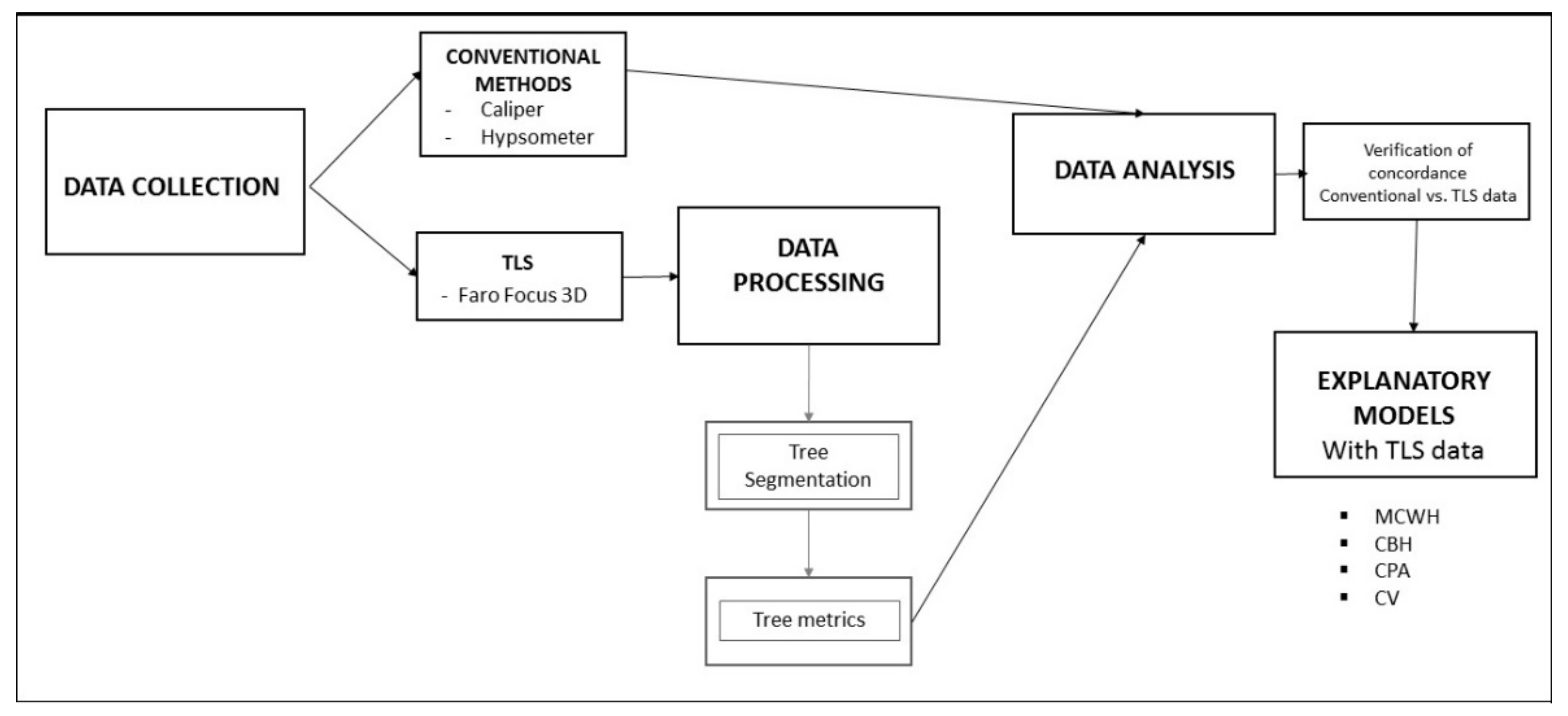
2.3. Data Processing

The Faro laser scanner creates .fls files. These files were opened and co-registered into one single point cloud file. xyz extension with the software Faro Scene Version 7.0 (Faro Technologies Inc., Lake Marry, FL, USA). Point clouds were imported to the module IMispect from Polyworks Version 12.1.3 software (InnovMetric Software Inc., Quebec, QC, Canada) [19,47,48] together with a .csv file with the UTM coordinates for each tree taken with the Total Station Topcon 220. Thereby, 3D images could be matched with each tree ID.

2.3.1. Tree Segmentation
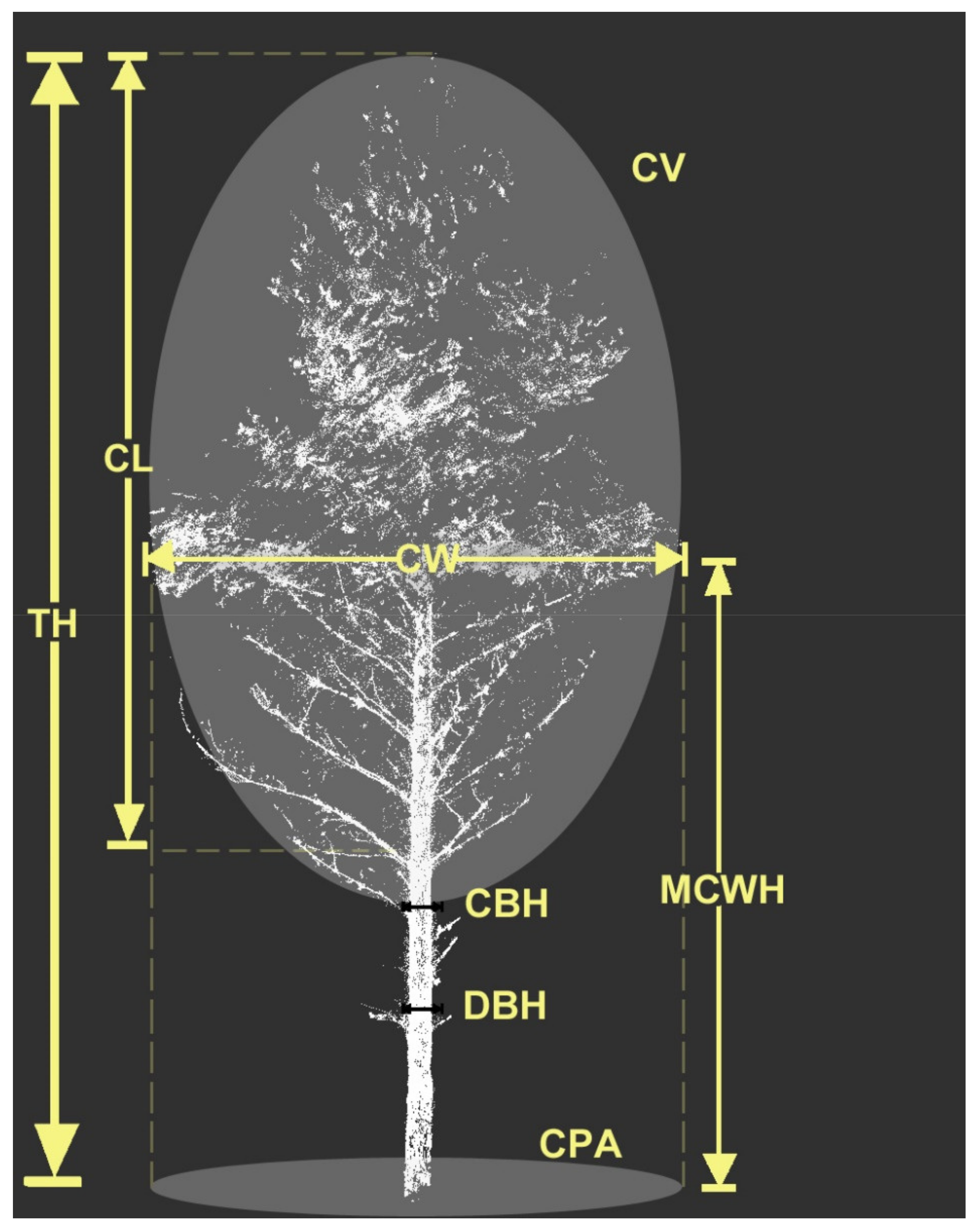
Tree segmentation consists of obtaining one point-cloud for each tree belonging to the plot, i.e., we should have as many point clouds as trees in the plot (Table 1). For Triplet 1, this isolation was conducted manually: we edited in IMispect the original point cloud selecting each tree and made a copy of the point cloud for each tree. Triplet 2 trees were first isolated by an algorithm developed by [39] which is based on density spatial clustering algorithm with noise (dbscan) function in the dbscan package of R [49] to detect individual-tree positions. Only the x- and y-axes are used as input data. From here, dbscan is automatically able to find each tree as a cluster, i.e., each recognized cluster (stem) now receives a unique number and can be processed individually. Ground points are recognized by dbscan as noise points because of the horizontal structure in contrast to the vertically grown stems. Then each cluster is individually queried as to, which stem base cluster is closest in distance and whether this distance is close enough (≤0.05 m) to be classified as associated points. After this step, each tree is visually checked for completeness. If necessary, unrecognized tree parts are added manually, and artefacts not belonging to the tree are removed using the software RiSCAN PRO. More detailed information is provided in [39].
In both cases, final refined data for each tree were needed and it was performed manually in IMispect by deleting points that were not part of the trees or by separating trees, that were identified as only one due to their crown proximity. All the trees belonging to the study plots were identified but due to canopy occlusion, especially in oak stands, which made tree separation impossible, the study was finally conducted with 91.2% of the total (Table 4).

2.3.2. Tree Metrics

TLS tree metrics were computed using the software “Mathematica 11” (Wolfram Research Inc., Champaign, IL, USA). In total, for each tree, we obtained eleven variables: Diameter at Breast Height (DBH), Total Height (TH), Lean, sweep and the crown metrics of: Crown base height (CBH), Maximum Crown Width Height (MCWH), Maximum Area, Crown Volume (CV), Crown Surface Area (CSA), Crown Length (CL), and asymmetry of the crown with respect to the stem (asymmetry) (Figure 3). An extensive description of the computing process can be found in [32]

2.4. Data Analysis

Data analysis was conducted using Rstudio. Inc. Version 1.1.453. Packages used were: dplyr [50], data.table [51], lme4 [52], broom [53], ggplot2 [54], psych [55], pastecs [56], car [57], gridExtra [58], nls2 [59], and tibble [60].
TLS data and conventional data were merged by tree ID. We checked the affinity of TLS data with the field data using the Kolmogorov-Smirnov test to test if conventional and TLS data are not significantly different for each studied variable and to prove equivalence and concordance of data, the Lin Concordance Correlation Coefficient [61] was conducted.
From this point, four models from TLS data were analyzed, setting as response variables Maximum Crown Width Height (MCWH) also known as height of maximum crown extension; Crown Base Height (CBH); Crown Projection Area (CPA); and Crown Volume (CV) the explanatory variables were categorized into four groups: size, density, competition, and mixture. Size category was defined by DBH and TH of target trees. To define density, we used Total Basal Area (BAtotal) of each tree, understanding density as competition at stand level. On the other hand, the competition was defined at tree level by the following variables: Largest Basal Area (BAL), both by species separately and total, Asymmetry [32] and the Hegyi Index [62], hereafter referred to as the Competition Index (CI). Finally, to define the mixture, we used the ratio variables of BA, BAL, and the total number of pine trees.
Density, competition, and mixture were defined for every single tree following [29]. The three radii sizes (5, 7.5, and 10 m) were chosen for two reasons: (1) our study plots are maximum 30 × 30 m; and (2) the influence radii for each tree is assumed to be between 1.5 and 2.5 times the target tree crown width (maximum in our sample is 7.41 m). Thanks to this, these three categories were not analyzed as categorical variables distinguishing between pure and mixed stands, but rather as continuous variables.

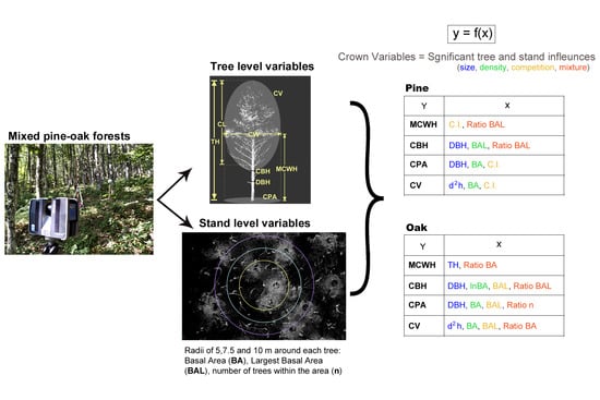
2.5. Explanatory Models

Based on forest modelling literature, different linear and non-linear models were tested to explain response crown variables (Table 5), adapting them to our four category explanatory variables (size, density, competition and mixture).
For the response variables -MCWH, CBH, and CPA- non-linear regression models were developed using brute force algorithm [59] and, for the CV variable, simple linear regression was used.
Before fitting models, correlations between explanatory variables were calculated and those that were highly correlated (ρ ≥ 0.9) were removed (oak ratio variables), to avoid multicollinearity problems. Thus, we used pine as a reference for the basal area, the number of trees per plot, and the BAL ratios. In addition, for CPA and CV response variables, the explanatory variable d2h (squared diameter at breast height times height) was included as a size variable since this variable represents a proxy for tree volume. Furthermore, for CPA response, the logarithmic transformation of Basal Area was included as a density explanatory variable, as in [63]
For each radius of influence considered (5, 7.5, and 10 m) all possible combinations of explanatory models (size, density, competition, and mixture) were tested. We unified all models performed with all influence radii for each response variable, with all resulting models ordered from the lowest to the highest Akaike coefficient (AIC). According to [64] the top five models with the lowest AIC index were selected. Finally, the best model for each response variable and species was selected if it had a coherent biological sense.

3. Results

3.1. Data Analyst

The Kolmogorov Smirnov test was not significant ( α = 0.05) and the Lin Concordance Correlation Coefficients for DBH and TH were 0.98 and 0.74, respectively, confirming the distribution of TLS data corresponding to the data taken in the field are consistent and have no significant differences. From then on, the following analysis was performed only with TLS data.
Firstly, descriptive statistics of all trees classified by species and pure and mix plots was performed (Table 6). We observed that oaks show similar tree heights, both in pure and mixed stands, but they are slightly thicker (DBH one cm higher) in the mix with pines than in pure conditions. Unlike pines, DBH is up to almost 3.5 cm thinner in the mix with pines but slightly taller (+0.5 m) compared to pure plots.

3.2. Explanatory Models

The best models selected according to the lowest Akaike index (AIC) and biological sense are shown in Table 7 and as equations in Table 8. For all cases, the best model selected was the model with the lowest AIC index, except for the MCWH variable in both species, where models with the second AIC index were selected due to the first ones having no biological sense.
We observed that the size of the tree is a significant variable for all cases, with only one exception, MCWH for pines. In all cases, tree size affected the crown shape the bigger the tree, the greater increase in growth of the CBH, MCWH, and their CPA and CV as well. That is to say, the bigger the tree, the higher and wider the crown will be. Competition boosted the MCWH and CPA of pines, but it is we observed for the rest of the variables competition has a negative effect on crown shapes for both species, as crowns were shorter and narrower.
The mixture variable is always significant for oaks. The presence of pines makes the height of the oaks’ crowns (MCWH and CBH) smaller, and by contrast, makes their crown projection and volume larger.

4. Discussion

In this study, we have obtained a more comprehensive understanding of pine-oaks forest dynamics thanks to the use of TLS. We have scanned six plots (two triplets) formed by Quercus petraea and Pinus sylvestris in pure (Two plots for each species) and mixed stands (Two plots). With the scanning four-crown variables: MCWH, CBH, CPA, and CV from a total of 193 pines and 256 oaks and later analyzed them by linear and non-linear regression using tree size, stand density, competition, and mixture proportion as explanatory variables (Table 5). Several models were fitted for each crown response variable, these models were selected by the lowest AIC index and biological sense (one for each species and variable). Results (Table 8) showed us that tree crowns occupy the gaps between species, and that mixture, competition, density and size play a significant role in the shape of the species’ crowns. Oak crowns remain under pines but are wider, while pine crowns are higher and narrower when interacting with oaks.

4.1. Mixing Affects Tree Size

Similar to [65] we observed differences in height and diameter of tree species growing in mixed stands vs. monocultures. We have found slightly higher TH for Scots Pines in mixed than in pure stands but no such pattern for their DBH. On the contrary, Sessile Oaks showed larger DBH in mixed stands, but their TH was slightly lower. This is to say that when in interaction, oaks are shorter but thicker and pines are thinner but taller. This explains a complementarity between pines and oaks within the mixed stands which could be related to specific growth strategies [35] when growing shade-tolerant species together with light-demanding species [66]; or to a more efficient use of resources over time [67], as interspecific competition for light decreases in the mixture [68] enabling changes in tree architecture and crown plasticity, and therefore, increase light capture and productivity [6,69]. Shade-tolerant oak trees utilize resources more efficiently in the mixture which could result even in higher radial increment rates [70]. Regarding this aspect, [66] found the higher productivity in Quercus petraea mixed stands when they grow together with light-demanding pioneer species with deeper roots features [71] as it is Pinus sylvestris.

4.2. Effect of Size, Density, Competition and Mixture on Species Crown Size

Our results suggest there are both competition and mixture effects on oaks and pines’ crown dimensions and shape (Table 8) suggesting that species mixing modifies the crown size and shape, and thereby the canopy space-filling [1]. Some researchers have hypothesized differences in crown shape between deciduous broadleaves and evergreen conifers are at the origin of a positive mixture effect on species productivity in broadleaved-conifer mixed stands [72]. Here, the models selected showed us there is a significant effect of size, density, competition, and mixture variables, either negative or positive on crown allometry. [66] highlighted that there exists either a competitive advantage of Q. petraea over a more light-demanding species, like Pinus sylvestris, or a result of the complementary use of resources in the mixture, as it is shown in Figure 4 where it is observed how at a same tree size for both species under two density scenarios (based on BAtotal), oak CPA vary less than pines.
Regarding mixture, explanatory models revealed that the presence of pines positively affected the crown expansion of oaks (expressed as CV and CPA). At the same time, crown elongation (expressed by CBH and MCWH) was negatively affected (Table 8). On the contrary, pines seem to have higher crowns when growing together with oaks or with bigger pines in the neighborhood (represented by the trees in the three radii considered). Pine crown expansion (CV and CPA) was not significantly affected by the mixture. Our findings suggest that crown oaks, in the presence of pines, remain under the crown pines, occupying the space between pine stems, that may be the reason why crown oaks are shorter but wider, contrary to pines where crowns start at a higher point when growing together with oaks.
Our results suggest a multi-layered canopy (stem diameter and height variety) in oaks-pines stands in Northern Spain. We hypothesize that multi-layered canopies are produced by the mixture complementarity of crown shapes of pines and oaks due to their differential crown architecture. On the one hand, shade-tolerant and shade-intolerant tree species combination [23,73], together with slower growth of oaks lead to differentiation in the canopy. Shade-tolerant species tend to have a crown shape optimized for the capture of light under limiting conditions [74], and in mixtures force non-tolerant species to grow to reach upper canopy level. Additionally, resource use complementarity appears when in winter the lack of leaves in oak allows pine trees to capture light and photosynthesize.
However, the mixture also limits light resources in summer creating interspecific competition, as we have seen in our analysis. This fact may cause changes in tree species crown allometry [66]. Our results suggest a complementarity in canopy space occupation; Oaks produce wider crowns and pines larger stems to be able to capture the light above oaks. This can be explained by differences in foliage persistence during the year [2], and by inter-specific variations in crown architecture and height, when combining species with different shade tolerances or vertically-oriented species with more laterally expanding tree species [5,12].
Finally, the origin of the forest, i.e., plantation or natural regeneration may affect trees and associated vegetation relative to those in monocultures [65], the same way we are seeing in our study combining pine plantation with natural oak resprouting where we have found trees’ neighborhood seems to be affecting crown allometry.
This apparent rapport between oaks growing together with pines may agree with relaxing resources competition in mixed forests that leads trees species to temporal diversification and spatial niche partitioning as suggested by [69] and [35]. Wider tree spacing reduced competition and increased resource acquisition capacity per tree, therefore facilitating crown expansion [31] as our models suggest for oaks.
Contrary [23] we have not found the density of shade-intolerant tree species to be the most significant explanatory variable in multiple regression. We found density only explains the CPA and CV of the trees. For these two variables, in line with [75] we saw that trees in stands with a higher BA exhibited greater CV and CPA for both oak and pine, creating a more heterogeneous stand structure.
This study is the most comprehensive work focused on the crown structure on Quercus petraea- Pinus sylvestris mixture contributing to the understanding of this very important mixture. Using TLS, we were able to focus on the crown structural pattern in great detail, in order to gain deeper insight into tree crowns’ response to pines and oaks mixture. We were able to quantify geometrical aspects of tree crown: Maximum Crown Width Height, Crown Base Height, Crown Projection Area, and Crown Volume that were conducted on a large number of trees (449 trees, 193 Scots Pines, and 256 Sessile Oak). Therefore, we have obtained rigorous information about crown differences between these two species and how their size, density, competition, and mixture around affect their crown shape, obtaining a plausible answer hidden behind the identified productivity changes between species as [13] stated for pine-pine mixtures. As discussed by [20], the characterization of crown species gives us information on how species tend to occupy the stand canopy and helps to quantify their plasticity. For instance, an increase in oak CPA and CV forces Scots pine trees nearby to raise their crowns to reach upper canopy levels. Unlike other deciduous species, which have a remarkable capacity to adjust their morphology and physiology to a particular set of light conditions [76].
The fitted models of this study suggest mixture increases stand structural complexity index as pointed in [31] due to better use of the available light [26] when growing shade-tolerant and intolerant species together. Our study plots had not been thinned in the last 10 years but previous silviculture could have caused a residual effect in our findings due to the memory effect found in the forest stand dynamic [16,77]. The origin of the forest, i.e., plantation or natural regeneration may affect trees and associated vegetation relative to those in monocultures [65]. In our study, combining pine plantation with natural oak resprouting where we have found trees’ neighborhood seems to be affecting crown allometry.
Long-term observation of mixed forests and general findings are still rare [8] especially when involving individual tree analysis [78]. Using detailed quantification of the crown can help to gain insight in differences in pure and mixed forests as a result of species’ interactions and to define sound management options.

5. Conclusions

Crown plasticity represents one of the species potential to acquire resources and occupy space [21]. In this study we investigated how the crown shapes of two widespread species in Europe, Pinus sylvestris and Quercus petraea, varied with tree size, density, competition, and mixture. We derived four response crown variables (Maximum Crown Width, Crown Base Height, Crown projection Area and Crown Volume) from TLS. Our two hypotheses were confirmed: (1) pines and oaks differ in size when they grow in mixed conditions compared to pure conditions; where pines are taller and thinner, and oaks are shorter and thicker; and (2) the models suggest that in mixtures with pine, oak crowns are shorter and wider while pine crowns are taller and narrower when growing with oaks. The models we developed provide accurate information on species interactions that can be implemented in forest simulators. This information will help forest managers to design more effective silvicultural prescriptions.

Author Contributions

Conceptualization, S.U., I.B., R.S.M. and F.B.; methodology, S.U., I.B., R.S.M., F.B., M.E., D.S.; validation and formal analysis, S.U., I.B., R.S.M. and F.B.; writing—original draft preparation, S.U.; writing—review and editing, S.U., I.B., R.S.M., M.E., D.S., and F.B.; supervision I.B., F.B.; project administration, F.B. All authors have read and agreed to the published version of the manuscript.

Funding

This work has financially supported by CARE4C H2020-MSCA-RISE-2017, Grant Agreement no. 778322 and by SMART VA183P20 - Bosques mixtos: Selvicultura, Mitigación, Adaptación, Resiliencia y Trade-offs (project code VA183P20) funded by the Castilla and León Regional Government (Spain) and the the European Regional Development Fund (ERDF).

Institutional Review Board Statement

Not applicable.

Informed Consent Statement

Not applicable.

Data Availability Statement

Data sharing not applicable.

Acknowledgments

This work was supported by the CARE4C H2020-MSCA-RISE-2017 (Grant Agreement no 778322) and, the research project SMART VA183P20 (Junta de Castilla y León) + FEDER. Sara Uzquiano’s work was supported by an FPI grant from Junta de Castilla y León and the European Social Fund 2014–2020. The author would like to acknowledge the Architectural Photogrammetry Laboratory (LFA) of the Architecture School of the University of Valladolid for all the TLS technical support given during the process of this study.

Conflicts of Interest

The authors declare no conflict of interest.

References

  1. Bauhus, J.; Forrester, D.I.; Pretzsch, H. Mixed-species forests: The development of a forest management paradigm. In Mixed-Species Forests: Ecology and Management; Springer: Berlin/Heidelberg, Germany, 2017; pp. 1–25. ISBN 9783662545539. [Google Scholar]
  2. Bravo, F.; Ariza, A.M.; Dugarsuren, N.; Ordóñez, C. Disentangling the Relationship between Tree Biomass Yield and Tree Diversity in Mediterranean Mixed Forests. Forests 2021, 12, 848. [Google Scholar] [CrossRef]
  3. Pretzsch, H.; Forrester, D.I. Stand Dynamics of Mixed-Species Stands Compared with Monocultures. In Mixed-Species Forests: Ecology and Management; Pretzsch, H., Forrester, D.I., Bauhus, J., Eds.; Springer Nature: Berlin, Germany, 2017; pp. 117–209. ISBN 9783662545515. [Google Scholar]
  4. Steckel, M.; del Río, M.; Heym, M.; Aldea, J.; Bielak, K.; Brazaitis, G.; Černý, J.; Coll, L.; Collet, C.; Ehbrecht, M.; et al. Species mixing reduces drought susceptibility of Scots pine (Pinus sylvestris L.) and oak (Quercus robur L., Quercus petraea (Matt.) Liebl.)—Site water supply and fertility modify the mixing effect. For. Ecol. Manag. 2020, 461, 117908. [Google Scholar] [CrossRef]
  5. Ammer, C. Diversity and forest productivity in a changing climate. New Phytol. 2019, 221, 50–66. [Google Scholar] [CrossRef] [Green Version]
  6. Gough, C.M.; Atkins, J.W.; Fahey, R.T.; Hardiman, B.S. High rates of primary production in structurally complex forests. Ecology 2019, 100, e02864. [Google Scholar] [CrossRef] [PubMed] [Green Version]
  7. Bravo-Oviedo, A.; Pretzsch, H.; Ammer, C.; Andenmatten, E.; Barbati, A.; Barreiro, S.; Brang, P.; Bravo, F.; Coll, L.; Corona, P.; et al. European Mixed Forests: Definition and research perspectives. For. Syst. 2014, 23, 518–533. [Google Scholar] [CrossRef]
  8. Pretzsch, H.; Forrester, D.I.; Bauhus, J. Modelling Mixed-Species Forest Stands. In Mixed-Species Forests: Ecology and Management; Pretzsch, H., Forrester, D.I., Bauhus, J., Eds.; Springer: Berlin, Germany, 2017; ISBN 9783662545515. [Google Scholar]
  9. Bayer, D.; Seifert, S.; Pretzsch, H. Structural crown properties of Norway spruce (Picea abies [L.] Karst.) and European beech (Fagus sylvatica [L.]) in mixed versus pure stands revealed by terrestrial laser scanning. Trees Struct. Funct. 2013, 27, 1035–1047. [Google Scholar] [CrossRef]
  10. Forrester, D.I.; Bauhus, J. A Review of Processes Behind Diversity—Productivity Relationships in Forests. Curr. For. Rep. 2016, 2, 45–61. [Google Scholar] [CrossRef] [Green Version]
  11. Liang, J.; Crowther, T.W.; Picard, N.; Wiser, S.; Zhou, M.; Alberti, G.; Schulze, E.-D.; McGuire, A.D.; Bozzato, F.; Pretzsch, H.; et al. Positive biodiversity-productivity relationship predominant in global forests. Science 2016, 354. [Google Scholar] [CrossRef] [PubMed] [Green Version]
  12. Pretzsch, H.; Schütze, G. Size-structure dynamics of mixed versus pure forest stands. For. Syst. 2014, 23, 560–572. [Google Scholar] [CrossRef] [Green Version]
  13. Riofrío, J.; Del Río, M.; Bravo, F. Mixing effects on growth efficiency in mixed pine forests. Forestry 2017, 90, 381–392. [Google Scholar] [CrossRef] [Green Version]
  14. Pretzsch, H. Canopy space filling and tree crown morphology in mixed-species stands compared with monocultures. For. Ecol. Manag. 2014, 327, 251–264. [Google Scholar] [CrossRef] [Green Version]
  15. Metz, J.Ô.; Seidel, D.; Schall, P.; Scheffer, D.; Schulze, E.D.; Ammer, C. Crown modeling by terrestrial laser scanning as an approach to assess the effect of aboveground intra- and interspecific competition on tree growth. For. Ecol. Manag. 2013, 310, 275–288. [Google Scholar] [CrossRef]
  16. Pretzsch, H. Forest Dynamics, Growth and Yield; Springer: Berlin, Germany, 2009; ISBN 9783540883067. [Google Scholar]
  17. Luoma, V.; Saarinen, N.; Kankare, V.; Tanhuanpää, T.; Kaartinen, H.; Kukko, A.; Holopainen, M.; Hyyppä, J.; Vastaranta, M. Examining changes in stem taper and volume growth with two-date 3D point clouds. Forests 2019, 10, 382. [Google Scholar] [CrossRef] [Green Version]
  18. Lin, W.; Meng, Y.; Qiu, Z.; Zhang, S.; Wu, J. Measurement and calculation of crown projection area and crown volume of individual trees based on 3D laser-scanned point-cloud data. Int. J. Remote Sens. 2017, 38, 1083–1100. [Google Scholar] [CrossRef]
  19. Barbeito, I.; Dassot, M.; Bayer, D.; Collet, C.; Drössler, L.; Löf, M.; Del Rio, M.; Ruiz-Peinado, R.; Forrester, D.I.; Bravo-Oviedo, A.; et al. Terrestrial laser scanning reveals differences in crown structure of Fagus sylvatica in mixed vs. pure European forests. For. Ecol. Manag. 2017, 405, 381–390. [Google Scholar] [CrossRef]
  20. Cattaneo, N.; Bravo-Oviedo, A.; Bravo, F. Analysis of tree interactions in a mixed Mediterranean pine stand using competition indices. Eur. J. For. Res. 2018, 137, 109–120. [Google Scholar] [CrossRef]
  21. Pretzsch, H. The Effect of Tree Crown Allometry on Community Dynamics in Mixed-Species Stands versus Monocultures. A Review and Perspectives for Modeling and Silvicultural Regulation. Forests 2019, 10, 810. [Google Scholar] [CrossRef] [Green Version]
  22. Disney, M.I.; Boni Vicari, M.; Burt, A.; Calders, K.; Lewis, S.L.; Raumonen, P.; Wilkes, P. Weighing trees with lasers: Advances, challenges and opportunities. Interface Focus 2018, 8, 20170048. [Google Scholar] [CrossRef] [Green Version]
  23. McElhinny, C.; Gibbons, P.; Brack, C.; Bauhus, J. Forest and woodland stand structural complexity: Its definition and measurement. For. Ecol. Manag. 2005, 218, 1–24. [Google Scholar] [CrossRef]
  24. Kern, C.C.; Montgomery, R.A.; Reich, P.B.; Strong, T.F. Canopy gap size influences niche partitioning of the ground-layer plant community in a northern temperate forest. J. Plant Ecol. 2013, 6, 101–112. [Google Scholar] [CrossRef] [Green Version]
  25. Seidel, D.; Beyer, F.; Hertel, D.; Fleck, S.; Leuschner, C. 3D-laser scanning: A non-destructive method for studying above- ground biomass and growth of juvenile trees. Agric. For. Meteorol. 2011, 151, 1305–1311. [Google Scholar] [CrossRef]
  26. Cattaneo, N.; Schneider, R.; Bravo, F.; Bravo-Oviedo, A. Inter-specific competition of tree congeners induces changes in crown architecture in Mediterranean pine mixtures. For. Ecol. Manag. 2020, 476, 118471. [Google Scholar] [CrossRef]
  27. Ehbrecht, M.; Schall, P.; Ammer, C.; Seidel, D. Quantifying stand structural complexity and its relationship with forest management, tree species diversity and microclimate. Agric. For. Meteorol. 2017, 242, 1–9. [Google Scholar] [CrossRef]
  28. Forrester, D.I.; Ammer, C.; Annighöfer, P.J.; Barbeito, I.; Bielak, K.; Bravo-Oviedo, A.; Coll, L.; del Río, M.; Drössler, L.; Heym, M.; et al. Effects of crown architecture and stand structure on light absorption in mixed and monospecific Fagus sylvatica and Pinus sylvestris forests along a productivity and climate gradient through Europe. J. Ecol. 2018, 106, 746–760. [Google Scholar] [CrossRef] [Green Version]
  29. Höwler, K.; Annighöfer, P.; Ammer, C.; Seidel, D. Competition improves quality-related external stem characteristics of Fagus sylvatica. Can. J. For. Res. 2017, 47, 1603–1613. [Google Scholar] [CrossRef]
  30. Jacobs, M.; Rais, A.; Pretzsch, H. How drought stress becomes visible upon detecting tree shape using terrestrial laser scanning (TLS). For. Ecol. Manag. 2021, 489, 118975. [Google Scholar] [CrossRef]
  31. Juchheim, J.; Ehbrecht, M.; Schall, P.; Ammer, C.; Seidel, D. Effect of tree species mixing on stand structural complexity. For. Int. J. For. Res. 2020, 93, 75–83. [Google Scholar] [CrossRef]
  32. Seidel, D.; Leuschner, C.; Müller, A.; Krause, B. Crown plasticity in mixed forests-Quantifying asymmetry as a measure of competition using terrestrial laser scanning. For. Ecol. Manag. 2011, 261, 2123–2132. [Google Scholar] [CrossRef]
  33. Weiskittel, A.R.; Hann, D.W.; Kershaw, J.A.J.; Vanclay, J.K. Forest Growth and Yield Modeling, 1st ed.; John Wiley & Sons: Hoboken, NY, USA, 2011; ISBN 9780470665008. [Google Scholar]
  34. Montero, G.; del Río, M.; Roig, S.; Rojo, A. Selvicultura de Pinus sylvestris L. In Compendio de Selvicultura Aplicada en España; MMA-INIA: Madrid, Spain, 2008; pp. 503–534. [Google Scholar]
  35. Aldea Mallo, J. Tree Growth Dynamic and Thinning response in Mediterranean Pine-Oak Forest Stands. PhD Thesis, Universidad de Valladolid, Valladolid, Spain, April 2018. [Google Scholar]
  36. Bauhus, J.; Forrester, D.I.; Pretzsch, H. From Observations to Evidence About Effects of Mixed-Species Stands. In Mixed-Species Forests: Ecology and Management; Pretzsch, H., Forrester, D.I., Bauhus, J., Eds.; Springer Nature: Berlin, Germany, 2017; pp. 27–72. ISBN 9783662545515. [Google Scholar]
  37. Del Río, M.; Pretzsch, H.; Ruíz-Peinado, R.; Ampoorter, E.; Annighöfer, P.; Barbeito, I.; Bielak, K.; Brazaitis, G.; Coll, L.; Drössler, L.; et al. Species interactions increase the temporal stability of community productivity in Pinus sylvestrisFagus sylvatica mixtures across Europe. J. Ecol. 2017, 105, 1032–1043. [Google Scholar] [CrossRef] [Green Version]
  38. Heym, M.; Ruíz-Peinado, R.; Del Río, M.; Bielak, K.; Forrester, D.I.; Dirnberger, G.; Barbeito, I.; Brazaitis, G.; Ruškytkė, I.; Coll, L.; et al. EuMIXFOR empirical forest mensuration and ring width data from pure and mixed stands of Scots pine (Pinus sylvestris L.) and European beech (Fagus sylvatica L.) through Europe. Ann. For. Sci. 2017, 74, 9. [Google Scholar] [CrossRef] [Green Version]
  39. Jacobs, M.; Rais, A.; Pretzsch, H. Analysis of stand density effects on the stem form of Norway spruce trees and volume miscalculation by traditional form factor equations using terrestrial laser scanning (TLS). Can. J. For. Res. 2020, 50, 51–64. [Google Scholar] [CrossRef]
  40. Del Río, M.; Sterba, H. Comparing volume growth in pure and mixed stands of Pinus sylvestris and Quercus pyrenaica. Ann. For. Sci. 2009. [Google Scholar] [CrossRef]
  41. Pretzsch, H.; Steckel, M.; Heym, M.; Biber, P.; Ammer, C.; Ehbrecht, M.; Bielak, K.; Bravo, F.; Ordóñez, C.; Collet, C.; et al. Stand growth and structure of mixed-species and monospecific stands of Scots pine (Pinus sylvestris L.) and oak (Q. robur L., Quercus petraea (Matt.) Liebl.) analysed along a productivity gradient through Europe. Eur. J. For. Res. 2020, 139, 349–367. [Google Scholar] [CrossRef] [Green Version]
  42. Stimm, K.; Heym, M.; Uhl, E.; Tretter, S.; Pretzsch, H. Height growth-related competitiveness of oak (Quercus petraea (Matt.) Liebl. and Quercus robur L.) under climate change in Central Europe. Is silvicultural assistance still required in mixed-species stands? For. Ecol. Manag. 2021, 482. [Google Scholar] [CrossRef]
  43. Clevenger, A.P.; Purroy, F.J.; Pelton, M.R. Food habits of brown bears (Ursus arctos) in the Cantabrian Mountains, Spain. J. Mammal. 1992, 73, 415–421. [Google Scholar] [CrossRef]
  44. Reque, J.A. Selvicultura de Quercus petraea L. y Quercus robur L. In Compendio de Selvicultura Aplicada en España; Serrada, R., Montero, G., Reque, J.A., Eds.; MMA-INIA: Madrid, Spain, 2008; pp. 745–772. [Google Scholar]
  45. Ruiz-Villar, H.; Morales-González, A.; Bombieri, G.; Zarzo-Arias, A.; Penteriani, V. Characterization of a brown bear aggregation during the hyperphagia period in the Cantabrian Mountains, NW Spain. Ursus 2019, 29, 93–100. [Google Scholar] [CrossRef]
  46. Vallet, P.; Perot, T. Coupling transversal and longitudinal models to better predict Quercus petraea and Pinus sylvestris stand growth under climate change. Agric. For. Meteorol. 2018, 263, 258–266. [Google Scholar] [CrossRef]
  47. Ferrarese, J.; Affleck, D.; Seielstad, C. Conifer crown profile models from terrestrial laser scanning. Silva Fenn. 2015, 49, 1–25. [Google Scholar] [CrossRef] [Green Version]
  48. Hackenberg, J.; Wassenberg, M.; Spiecker, H.; Sun, D. Non Destructive Method for Biomass Prediction Combining TLS Derived Tree Volume and Wood Density. Forests 2015, 6, 1274–1300. [Google Scholar] [CrossRef]
  49. Hahsler, M.; Piekenbrock, M.; Doran, D. CRAN—Package dbscan. Available online: https://cran.r-project.org/web/packages/dbscan/index.html (accessed on 3 December 2021).
  50. Hadley, W.; Romain, F.; Lionel, H.; Kirill, M. CRAN—Package dplyr. Available online: https://cran.r-project.org/web/packages/dplyr/index.html (accessed on 3 December 2021).
  51. Dowle, M.; Srinivasan, A. CRAN—Package Data Table. Available online: https://cran.r-project.org/web/packages/data.table/index.html (accessed on 3 December 2021).
  52. Bates, D.; Maechler, M.; Bolker, B.; Walker, S. CRAN—Package lme4. Available online: https://cran.r-project.org/web/packages/lme4/index.html (accessed on 3 December 2021).
  53. Robinson, D.; Hayes, A.; Couch, S. CRAN—Package Broom. Available online: https://cran.r-project.org/web/packages/broom/index.html (accessed on 3 December 2021).
  54. Wickham, H. CRAN—Package ggplot2. Available online: https://cran.r-project.org/web/packages/ggplot2/index.html (accessed on 3 December 2021).
  55. Revelle, W. CRAN—Package Psych. Available online: https://cran.r-project.org/web/packages/psych/index.html (accessed on 3 December 2021).
  56. Grosjean, P.; Ibanez, F. CRAN—Package Pastecs. Available online: https://cran.r-project.org/web/packages/pastecs/index.html (accessed on 3 December 2021).
  57. Fox, J.; Weisberg, S. CRAN—Package Car. Available online: https://cran.r-project.org/web/packages/car/index.html (accessed on 3 December 2021).
  58. Auguie, B. CRAN—Package gridExtra. Available online: https://cran.r-project.org/web/packages/gridExtra/index.html (accessed on 3 December 2021).
  59. Grothendieck, G. CRAN—Package nls2. Available online: https://cran.r-project.org/web/packages/nls2/index.html (accessed on 3 December 2021).
  60. Müller, K.; Wickham, H. CRAN—Package Tibble. Available online: https://cran.r-project.org/web/packages/tibble/index.html (accessed on 3 December 2021).
  61. Lin, L.I. A Concordance Correlation Coefficient to Evaluate Reproducibility. Biometrics 1989, 45, 255–268. Available online: http://0-www-jstor-org.brum.beds.ac.uk/stable/2532051 (accessed on 8 September 2021). [CrossRef]
  62. Hegyi, F. A simulation model for managing jack-pine stands. In Growth Models for Tree and Stand Simulation: Proceedings of Meetings in 1973. International Union of Forestry Research Organizations. Working Party S4.01; Fries, J., Ed.; Skogshögskolan: Stockholm, Sweden, 1974; pp. 74–99. [Google Scholar]
  63. Ritter, T.; Nothdurft, A. Automatic assessment of crown projection area on single trees and stand-level, based on three-dimensional point clouds derived from terrestrial laser-scanning. Forests 2018, 9, 237. [Google Scholar] [CrossRef] [Green Version]
  64. Johnson, J.B.; Omland, K.S. Model selection in ecology and evolution. Trends Ecol. Evol. 2004, 19, 101–108. [Google Scholar] [CrossRef] [PubMed]
  65. Himes, A.; Puettmann, K. Tree species diversity and composition relationship to biomass, understory community, and crown architecture in intensively managed plantations of the coastal Pacific Northwest, USA. Can. J. For. Res. 2020, 50, 1–12. [Google Scholar] [CrossRef]
  66. Toïgo, M.; Perot, T.; Courbaud, B.; Castagneyrol, B.; Gégout, J.C.; Longuetaud, F.; Jactel, H.; Vallet, P. Difference in shade tolerance drives the mixture effect on oak productivity. J. Ecol. 2018, 106, 1073–1082. [Google Scholar] [CrossRef]
  67. Forrester, D.I. The spatial and temporal dynamics of species interactions in mixed-species forests: From pattern to process. For. Ecol. Manag. 2014, 312, 282–292. [Google Scholar] [CrossRef]
  68. Jucker, T.; Bouriaud, O.; Coomes, D.A. Crown plasticity enables trees to optimize canopy packing in mixed-species forests. Funct. Ecol. 2015, 29, 1078–1086. [Google Scholar] [CrossRef] [Green Version]
  69. Williams, L.J.; Paquette, A.; Cavender-Bares, J.; Messier, C.; Reich, P.B. Spatial complementarity in tree crowns explains overyielding in species mixtures. Nat. Ecol. Evol. 2017, 1, 1–7. [Google Scholar] [CrossRef] [PubMed]
  70. Cuny, H.E.; Rathgeber, C.B.K.; Lebourgeois, F.; Fortin, M.; Fournier, M. Life strategies in intra-annual dynamics of wood formation: Example of three conifer species in a temperate forest in north-east France. Tree Physiol. 2012, 32, 612–625. [Google Scholar] [CrossRef] [Green Version]
  71. Sánchez-Costa, E.; Poyatos, R.; Sabaté, S. Contrasting growth and water use strategies in four co-occurring Mediterranean tree species revealed by concurrent measurements of sap flow and stem diameter variations. Agric. For. Meteorol. 2015, 207, 24–37. [Google Scholar] [CrossRef] [Green Version]
  72. Pretzsch, H.; Schütze, G. Transgressive overyielding in mixed compared with pure stands of Norway spruce and European beech in Central Europe: Evidence on stand level and explanation on individual tree level. Eur. J. For. Res. 2009, 128, 183–204. [Google Scholar] [CrossRef]
  73. Pretzsch, H.; del Río, M.; Schütze, G.; Ammer, C.; Annighöfer, P.; Avdagic, A.; Barbeito, I.; Bielak, K.; Brazaitis, G.; Coll, L.; et al. Mixing of Scots pine (Pinus sylvestris L.) and European beech (Fagus sylvatica L.) enhances structural heterogeneity, And the effect increases with water availability. For. Ecol. Manag. 2016, 373, 149–166. [Google Scholar] [CrossRef] [Green Version]
  74. Aiba, M.; Nakashizuka, T. Architectural differences associated with adult stature and wood density in 30 temperate tree species. Funct. Ecol. 2008, 23, 265–273. [Google Scholar] [CrossRef]
  75. Juchheim, J.; Ammer, C.; Schall, P.; Seidel, D. Canopy space filling rather than conventional measures of structural diversity explains productivity of beech stands. For. Ecol. Manag. 2017, 395, 19–26. [Google Scholar] [CrossRef]
  76. Delagrange, S.; Montpied, P.; Dreyer, E.; Messier, C.; Sinoquet, H. Does shade improve light interception efficiency? A comparison among seedlings from shade-tolerant and -intolerant temperate deciduous tree species. New Phytol. 2006, 172, 293–304. [Google Scholar] [CrossRef] [Green Version]
  77. Lara, W.; Bravo, F.; Maguire, D.A. Modeling patterns between drought and tree biomass growth from dendrochronological data: A multilevel approach. Agric. For. Meteorol. 2013, 178–179, 140–151. [Google Scholar] [CrossRef]
  78. Uria-Diez, J.; Pommerening, A. Crown plasticity in Scots pine (Pinus sylvestris L.) as a strategy of adaptation to competition and environmental factors. Ecol. Modell. 2017, 356, 117–126. [Google Scholar] [CrossRef]
Figure 1. Location of study plots. White dots represent the corner of each plot and the numbers next to them stand for their plot ID.
Remotesensing 13 04955 g001
Figure 2. Work diagram. MCWH = Maximum Crown Width Height; CBH = Crown Base Height; CPA = Crown Projection Area, CV = Crown Volume.
Remotesensing 13 04955 g002
Figure 3. Variables computed for each tree by “Mathematica11” software. TH = Total Height; CL = Crown Length; CW = Crown Width; CBH = Crown Base Height; DBH= Diameter at Breast Height; CPA = Crown Projection Area; MCWH= Maximum Crown Width Height; CV = Crown Volume.
Remotesensing 13 04955 g003
Figure 4. Scatterplot with observed data for CPA and simulation of tree sizes of DBH in both pines and oaks, 15, 30, and 45 cm. The solid line represents predicted CPA with a high value of BA and the dashed line with a low value of BA.
Remotesensing 13 04955 g004
Table 1. Inventory data of oak-pine triplets where stand indicates plot condition (pure or mixed) and the letters Ps and Qp stand for Pinus sylvestris and Quercus petraea respectively. n represents the total number of trees within each plot; n pines is the number of Pinus sylvestris, n oaks is the number of Quercus petraea, and n other is the number of other species within the plots different from pines and oaks. Pines% and Oaks% represent the percentage of pines and oaks within each plot.
TripletPlot IDPlot Size (m)Standn/Plotn Pinesn Oaksn Other
1125 × 25pure-Ps70637--
730 × 30pure-Qp10208715
425 × 25mix-PsQp10348552
2230 × 30pure_Ps785721--
520 × 30pure-Qp85481--
630 × 30mix-PsQp1074463--
TOTAL54521631417
Table 2. Stand characteristics of the study species taken with conventional methods. n stands for number of total tree species. DBH is the Diameter at Breast Height in cm. TH is the total height of the tree in m. CBH is the Crown Base Height in m. CPA is the Crown Projection Area in cm2, and BA is the basal area in m2/ha.
Main Tree Species
Pine Oak
n = 216 n = 314
min13.60 7.20
DBH (cm)mean (± SD)29.69±6.6119.91±6.51
Median29.73 19.65
Max53.35 60.50
min10.50 4.00
TH (m)mean (± SD)18.23±1.9017.32±2.93
Median18.60 18.00
Max23.90 23.70
min1.10 2.00
mean (± SD)12.56±2.0811.67±2.21
CBH (m)Median12.70 12.00
Max17.50 16.70
min0.59 0.14
mean (± SD)12.50±8.809.88±9.37
CPA (m2)Median10.71 7.49
Max56.61 114.20
min0.17 0.06
mean (± SD)0.92±0.410.50±0.40
BA (m2/ha)Median0.90 0.43
Max2.49 4.96
Table 3. TLS measurement settings used to record the study plots.
Angular resolution0.6135 miliradHorizontal field of view0°–360°
OversamplingVertical field of view−60°–90°
Scan duration (mm:ss)approx. 02:08Point distance7.670 mm @ 10m
Scan size (Pt)8192 × 3414
Table 4. Total trees per plot compared to total point cloud trees isolated (TLS tree).
TripletPlotTypeSurfaceSpeciesn/PlotTLS Trees
11pure25 × 25Pine6361
7pure25 × 25Oak8775
4mixed30 × 30Pine-Oak48–5547–53
22pure30 × 30Pine5747
5pure20 × 30Oak8174
6mixed30 × 30Pine-Oak44–6338–54
Total498449
Table 5. Explanatory models defined for this study. s = size, d = density, c = competition and m = mixture, α0 = intercept, α1−4 = parameters of each coefficient (s, d, c, and m respectively), εi = error.
ModelsAuthor
M C W H = T H 1 + e α 0 * s + α 1 d + α 3 c + α 4 m + ε i (Pain and Hann, 1982)
C B H = M C W H 1 + e α 0 d s + α 1 d + α 3 c + α 4 m + ε i (Hann et al., 2003)
C P A = e α 0 + α 1 s + α 2 d + α 3 c + α 4 m + ε i (Ritter and Nothdurft, 2018)
C V = α 0 + α 1 s + α 2 d + α 3 c + α 4 m + ε i (Sanquetta et al., 2015)
Table 6. Mean Diameter Breast Height (DBH) in cm and Total height (TH) in m of trees calculated with TLS separated by species and kind of plot (pure or mix). n total is the total number of trees measured.
SpeciesPlotn TotalDBH (cm)TH (m)
MaxMean SDMinMaxMean SDMin
PinePure11346.9830.99±2.075.6826.4417.33±6.9711.62
Mix8447.3427.51±2.1313.9622.3618.04±6.3311.31
OakPure15561.2919.5±3.387.5623.217.38±7.426.39
Mix10733.5220.53±2.4110.0720.8517.31±5.208.73
Table 7. The explanatory models selected as the best fit according to their lowest Akaike index and biological criteria for each response variable (Variable) and species. r = radius of influence (5, 7.5 and 10 m); s = size; d = density; c = competition; m = mixture; α0 = intercept; α1-4 = the coefficient numbers for each explanatory variable (size, density, competition, and mixture); AIC = Akaike; K-S test = p-value of Kolmogorov-Smirnov test for residuals; R2 = coefficient of determination of the model.
VariableSpeciesrsdcmα0α1α2α3α4AICK-S TestR2
MCWHP. sylvestris10 CIRatio BALpine −0.11−1.13646.590.0780.54
Q. petraea10TH Ratio BApine −0.095 0.273890.470.0070.78
CBHP. sylvestris5DBH BALpineRatio BALpine −22.87 0.1−0.41557.210.2270.71
Q. petraea10DBHln
(BAtotal)
BALtotalRatio BALpine −14.430.050.040.17936.910.5430.74
CPAP. sylvestris10DBHBAtotalCI 0.06550.0188−0.0964 981.450.1940.66
Q. petraea7.5DBHBAtotalBALtotalRatio npine0.810.0390.089−0.1861.1541203.110.0010.70
CVP. sylvestris10d2 HBAtotalCI. 0.00150.442.35 1491.120.1000.55
Q. petraea7.5d2 HBAtotalBALpineRatio BA−20.280.0031.03−4.2946.921904.90.0100.64
Table 8. Final equations for each species and crown response variable.
Equation
MCWHPine M C W H = T H 1 + e 0.11 · C . I . 0.13 · R a t i o B A L p i n e
Oak M C W H = T H 1 + e 0.09 · T H + 0.28 · R a t i o B A p i n e
CBHPine C B H = M C W H 1 + e 22.9 · B A t o t a l D B H 0.1 · B A p i n e 0.41 · R A t i o B A L p i n e
Oak C B H = M C W H 1 + e 14.43 · B A t o t a l D B H + 0.05 · l n B A t o t a l + 0.04 · B A L t o t a l + 0.17 · R A t i o B A L p i n e
CPAPine C P A = e 0.07 · D B H + 0.02 · B A t o t a l 0.1 · C . I .
Oak C P A = e 0.9 + 0.04 · D B H + 0.09 · B A t o t a l 0.1 · B A L . t o t a l + 1.15 · R a t i o   n   p i n e
CVPine C V = 1.5 e 3 · d 2 h + 0.44 · B A t o t a l 2.35 · C . I .
Oak C V = 20.28 + 0.003 · d 2 h + 1.03 · B A t o t a l 4.29 · B A L t o t a l + 46.92 · R a t i o B A p i n e
Publisher’s Note: MDPI stays neutral with regard to jurisdictional claims in published maps and institutional affiliations.

