
Deep Learning Application to Surface Properties Retrieval Using TIR Measurements: A Fast Forward/Reverse Scheme to Deal with Big Data Analysis from New Satellite Generations

 , , and
Abstract
:
1. Introduction
2. Materials and Methods
2.1. Used Datasets
2.1.1. DART Dataset
- Maizefields: the DART maize mock-ups are simulated using parameters that vary around those measured in the maize fields of Barrax (Spain) during the Sentinel-3 experimental campaign carried out by ESA (project SEN3EXP: https://earth.esa.int/eogateway/campaigns/sen3exp, accessed on 2 December 2021) in June–July 2009. Each mock-up is made of the spatial distribution of clones of a single 3D maize plant at a specific growth stage in terms of height and number of leaves, with some variability (e.g., small random azimuthal rotation of the plant). Three standard growth stages are considered according to the Biologische Bundesanstalt, Bundessortenamt, and CHemical industry (BBCH) scale (https://www.openagrar.de/receive/openagrar_mods_00042351, accessed on 2 December 2021). Each maize plant is duplicated along rows with specific distances between plants and rows and is also rotated so that its leaf mean azimuthal direction is perpendicular to the rows. The density of plants combined with the leaf area of each 3D maize plant gives the leaf area density per ground surface (i.e., leaf area index: LAI). Three-row orientations (0, 45, 90) were simulated to consider the influence of sun rays on the distribution of shadows, and consequently on the spatial distribution of leaf and ground thermodynamic temperature. In all, we have 4,082,400 BOA and TOA maize spectra of 1200 bands: 28 viewing directions, five sun directions, three-leaf emissivity spectra, three ground emissivity spectra, three LAI values, three-row orientations, three ranges of leaf thermodynamic temperature (291 K to 315 K), three ranges of ground thermodynamic temperature (283 K to 323 K), two extreme profiles of atmosphere temperature, two extreme aerosol optical depths, and five atmosphere water vapor contents (from 0.9 g/cm to 6 g/cm).
- Wheatfields: they were simulated with the same configurations as the maize fields, apart from the fact that the row effects were not directly simulated. Indeed, DART created wheat 3D mock-ups by importing wheat fields simulated with the “Plantgen-ADEL” model for 500, 700, and 900 degree days ([15,16,17,18]). In all, we have 1,360,800 BOA and TOA wheat spectra of 1200 bands.
2.1.2. TASI Dataset
2.2. Datasets and Algorithms
2.2.1. Data Preparation: TASI-to-DART: Algorithm Description, Data Selection
- 1.
- Atmospheric composition: We used European Centre for Medium-range Weather Forecasts (ECMWF) daily profiles of altitude, temperature, pressure, ozone (O), and water vapor volume mixing ratios at 12:00 a.m. All other gases are taken from the IG2 database [25] for mid-latitude in July.
- 2.
- Surface characterization: Emissivity is obtained from TASI LSE retrieval. TASI measurements and LSE retrievals cover up to 11.5 µm. To produce emissivity values up to 13 µm, we extend the value of emissivity at 11.5 µm as we notice that this approximation is valid in most cases. LST is also taken from TASI retrieval. The surface is treated as Lambertian.
2.2.2. Data Augmentation
- 1.
- GANDART (GANs DART):The dataset used for training the GANDART is obtained by preprocessing the original DART dataset, cutting the spectra between 8 and 13 µm (900 points instead of 1200 spectral points as in the original dataset) and reshaping from 1D to 2D. The outputs are stacked in three layers for each sample composed of BOA radiance, TOA radiance, and down-looking irradiance. Then, a final scaling between −1 and 1 is performed. GANs are generally superior to AE for data generation. However, they are particularly hard to work with, as they require a lot of data and tuning. Moreover, GANs suffer from a lot of failure modes, and training them is challenging.The GAN developed for the generation of DART signatures adopts a model called Progressive Growing of GANs (PGGANs) [26].PGGANs is an innovative architecture in which the network is progressively trained to grow the dimension of the input. Hence, PGGANs introduce a new effective training approach. The neural network architecture does not change (parameters are the same) and there are no modifications with respect to the vanilla GANs model [6].The generative model starts the training at very low resolution (usually 4 × 4) and keeps improving at a fixed number of iterations (600 k following the original implementation). The resolution is doubled with a fixed schedule. We scale the resolution results in a transition period where the new convolutional layer is added to the network progressively, using a shortcut, similar to that in architectures such as residual networks [27].The advantages of this approach are mainly the reduced training time due to the progressive structure of the network and the sample accuracy. We adopt this architecture to both allow the fast generation of synthetic signatures without requiring long simulation runs and increase the number of samples to train on the deep learning-based inversion model. The algorithm takes about 0.57 s to generate one signature.The GANDART generator is able to create new samples (without a simulation required) to be used for training the deep learning-based inversion model or for directly performing a retrieval. The obtained training set has a 2D dimension (30 × 30 × 3) ready to be fed to the PGGANs model. A postprocessor reshapes the output of the generated samples, obtaining a 1-dimensional output of (900 × 3, respectively BOA, TOA, and downward irradiance at BOA).The updated version of PGGANs was initially implemented by [26] with StyleGAN. The proposed model introduced major improvements with respect to the original PGGANs. It maintained the progressive technology, reducing the training time. However, a series of changes are made:
- (a)
- Introduction of a controllable and discrete latent space. The input vector is firstly mapped into a multilayer fully connected neural network, avoiding inconsistencies in replicating the original data distribution.
- (b)
- Gaussian noise is introduced to each convolutional layer, making it controllable during both training and inference phases. Stochasticity due to Gaussian noise-induced learning, fine-grained details, increasing accuracy of generated samples.
- (c)
- Custom CUDA-optimized operations to perform on GPU, reducing the computation time and optimizing the batch size.
The training process is the one presented in the original paper with progressive growth of the resolution of the input samples according to Figure 1b of [28]. Preliminarily, the training phase of StyleGAN took almost 3 h using four Nvidia Tesla V100 GPUs. The maize scenario was used for an initial test phase where the maximum mean square error (MSE) obtained was of the order of 0.1%. An example of generated TOA and BOA radiances for the wheat case is reported in Figure 5. Finally, 1024 GANDART spectra are generated with StyleGAN. Although StyleGAN is the final choice, during the work, different techniques were tested to find the most suitable one. Table A1 in Appendix A reports all the tested techniques and the considerations that motivate our choice. - 2.
- TASI to DART AutoEncoder (TASI2DART):The dataset used to train the TASI2DART model for data augmentation is the TASI-to-DART (Section 2.2.1). As said, due to the size of the original dataset, the AE is preferable in this case for data generation. As for the DART dataset, the first step is to cut the spectra between 8 and 13 µm (900 spectral points). Then, the 900 spectral points are upsampled to 1024 to perform a reshape to 64 × 64 required to leverage the two-dimensional convolutions of the AE used and to perform transfer learning on the pretrained EfficientNet B1 used for the feature extraction. A common 70/30 split is used for cross-validating the metrics of the AE. As output for the training phase, there are 600 couples for the training and 250 couples for the cross-validation. For the preprocessing of the dataset, standardization is performed (mean equal to zero, standard deviation equal to one). This additional task avoids inconsistency during the training phase. Moreover, standardization ensures a proper activation of the neurons within the neural network. The AE is composed of three main components [29]:
- the encoder, which extracts significant characteristics of the original dataset to the space of representations or latent space. This AE uses as encoder an EfficientNet B1 for feature extraction [30]. The objective of the network is neural network scaling, increasing the accuracy [30]. Defined as compound model scaling, it is a grid-search method for efficiently retrieving the number of parameters of a neural network considering three main neural network variables (Figure 2 of [30]):
- -
- the width (w, number of channels for each hidden layer).
- -
- the resolution (r, the input resolution of the network).
- -
- the depth (d, number of hidden layers).
The objective of the scaling is to maximize the accuracy of the ImageNet classification dataset [31]. - Latent space: Inside the latent space resides all the high-level characteristics of the original dataset;
- A decoder: Re-expands the latent space to the target two-dimensional target.
2.2.3. Data Verification
- Descriptive data analysis, which uses tools to summarize and has measurements of properties such as tendency and dispersion of data (mean, median).
- Exploratory data analysis (EDA), which summarizes the main characteristics with visual methods to perform initial investigations on data to check assumptions and discover patterns and anomalies.
2.2.4. Retrieval Algorithms
- 1.
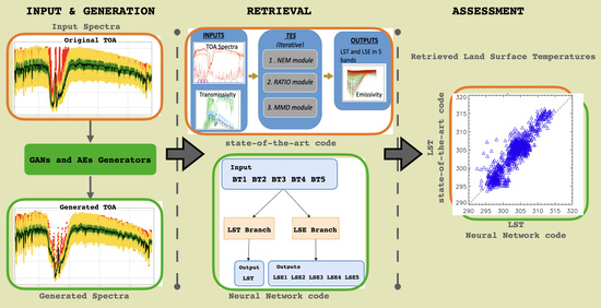
- TES algorithm:The TES algorithm is one of the state-of-the-art algorithms used for the retrieval of LST and LSE from aircraft and satellite missions. One of the main advantages of this algorithm is the capability to simultaneously retrieve LSE and LST. The algorithm is composed of three modules: (1) the normalized emissivity module (NEM), (2) the ratio module, and (3) the maximum–minimum difference module (MMD). The MMD module links the minimum value of the emissivity to the emissivity spectral contrast calculated as maximum-minimum emissivity. This relation depends on the instrument’s channels and the emissivity database used for the calculations. The MMD module is, then, critical for the correct determination of retrieved values. A complete description of the TES algorithm is beyond our scope and can be found in [34].The inputs of the TES algorithm are the BOA and the downward atmospheric irradiance at BOA, while the outputs are LSE in the instrument’s channels and LST.Generally, the TES inputs are obtained from TOA through the use of a RTM model. In our case, both the DART dataset and the TASI-to-DART dataset and the augmented ones already provide these two quantities; thus, they will be directly used (i.e., the TOA information is not used).As a first step, the signatures of BOA and downward irradiance are converted into BTs and convolved with SRFs for the five TIR channels.The second step is the addition of noise to the channel BTs. As we use BOA as TES input, we need to add the corresponding noise contribution to BOA instead of TOA, and this has an impact on the way the noise is added. The noise contribution that is transferred from TOA to BOA is given by the TOA noise contribution divided by the atmospheric transmissivity.As stated, the MMD module is critical for LSE and LST determination. Generally, MMD relation can be calculated through the use of emissivity laboratory spectra convolved with SRF. However, the scope of this work is to assess the performances of NN with respect to state-of-the-art codes. Thus, the auxiliary information used by the codes should be the same. For this reason, instead of using laboratory emissivity spectra for the calculation of TES MMD relation, we prefer to use the emissivity spectra contained in the DART and TASI-to-DART datasets. This means that the TES method does not use additional information not used by NN. This ensures that the differences in retrieved products are only due to the used methods and not to auxiliary information.
- 2.
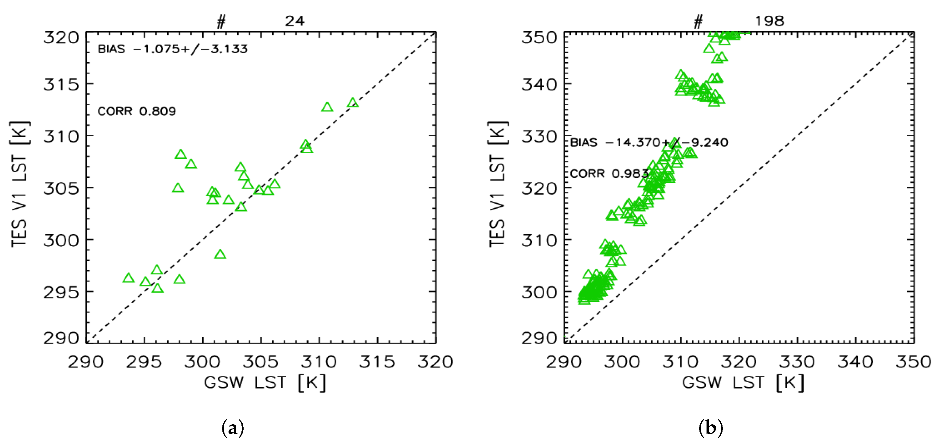
- GSW algorithm:The GSW algorithm exploits the relation between LST and the BTs at 11 and 12 µm [35]. No emissivity retrieval is performed. The relation that links LST and BTs at 11 and 12 µm is given by seven retrieval coefficients. It is obtained through the use of a RTM and depends on water vapor and satellite viewing angle. As, in this case, the algorithm exploits the TOA BTs, the noise is added directly onto TOA radiances. We use the same noise scenario adopted for the TES algorithm. In this work, the seven retrieval coefficients are obtained using a part of the simulations performed for the dataset creation (e.g., part of the TASI-to-DART dataset). The mean emissivity value and emissivity contrast required by GSW are calculated as the mean and contrast value of the TASI LSE retrievals used for the coefficient calculations. To obtain the seven retrieval coefficients, we use a least-square regression model. This type of algorithm is used, e.g., for trend calculations (e.g., [36]). The output of this model is shown in Figure 1a. Here, the observed LST values of the TASI training dataset are reported as red triangles as a function of the case number. The black line is the result of the least square fit obtained with the calculated retrieval coefficients. As can be noticed, we obtain a generally good agreement between simulations and observations, highlighting that the retrieved coefficients well reproduce LST–BTs relation.
- 3.
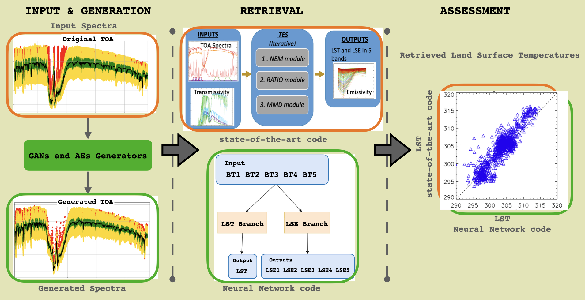
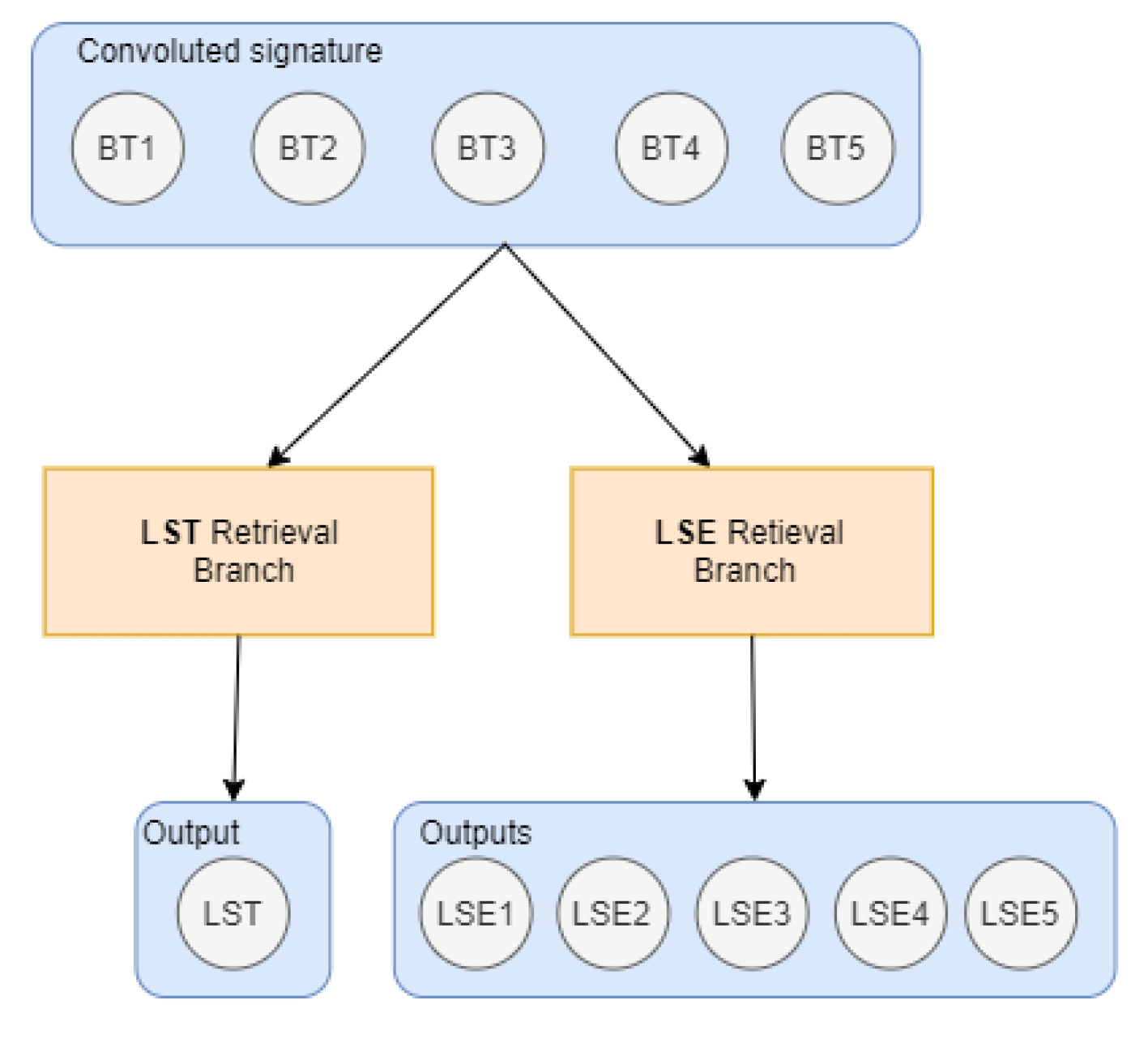
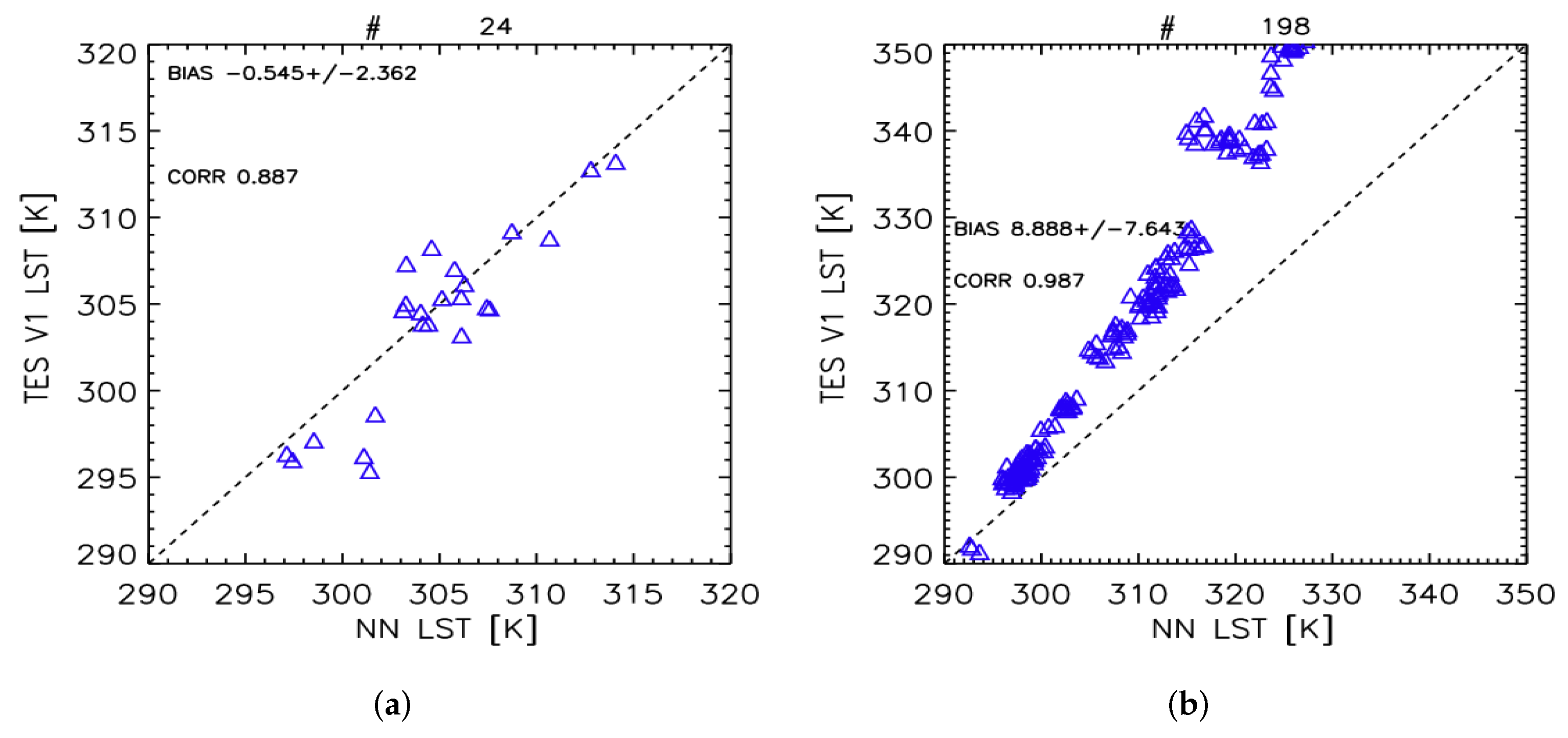
- Deep learning inversion model (DLIM):Deep learning techniques can be an alternative to state-of-the-art methods to perform satellite retrievals.Even if in this work we focused on LST retrievals, for completeness, the developed deep learning model, called the deep learning inversion model (DLIM), is conceived to also retrieve the LSE fields. The model has two branches: one dedicated to LST retrieval (feed-forward NN) and the other one for LSE retrieval (autoencoder) as reported in Figure 2. This happens because the values range of LST and LSE are different: LST falls in the range of hundreds of kelvins, while LSE is in a range between 0.7–1.0.Regarding the LST retrieval branch, a feed-forward neural network is selected because the problem perfectly corresponds to a regression problem. The LST branch is made of one dense layer with six neurons and one output layer with one neuron to compute the LST value.NN is trained using stochastic gradient descent and requires a loss (or cost) function when designing and configuring the model. As a loss function, the MAE for the five values of LSE and the MSE for the LST value is used. As the last step, the dataset is split into 70% training and 30% test with a validation split of 30%. For the train/evaluation phase, MAE is adopted as a metric for checking the consistency of the model. The optimizer is an Adam Optimizer [37] and the training epochs (cycles of NN training) are set to 2000 with early stopping callbacks based on validation loss (Figure 3). The list of different techniques tested to obtain the final results are reported in Table A1 in Appendix A.
3. Results
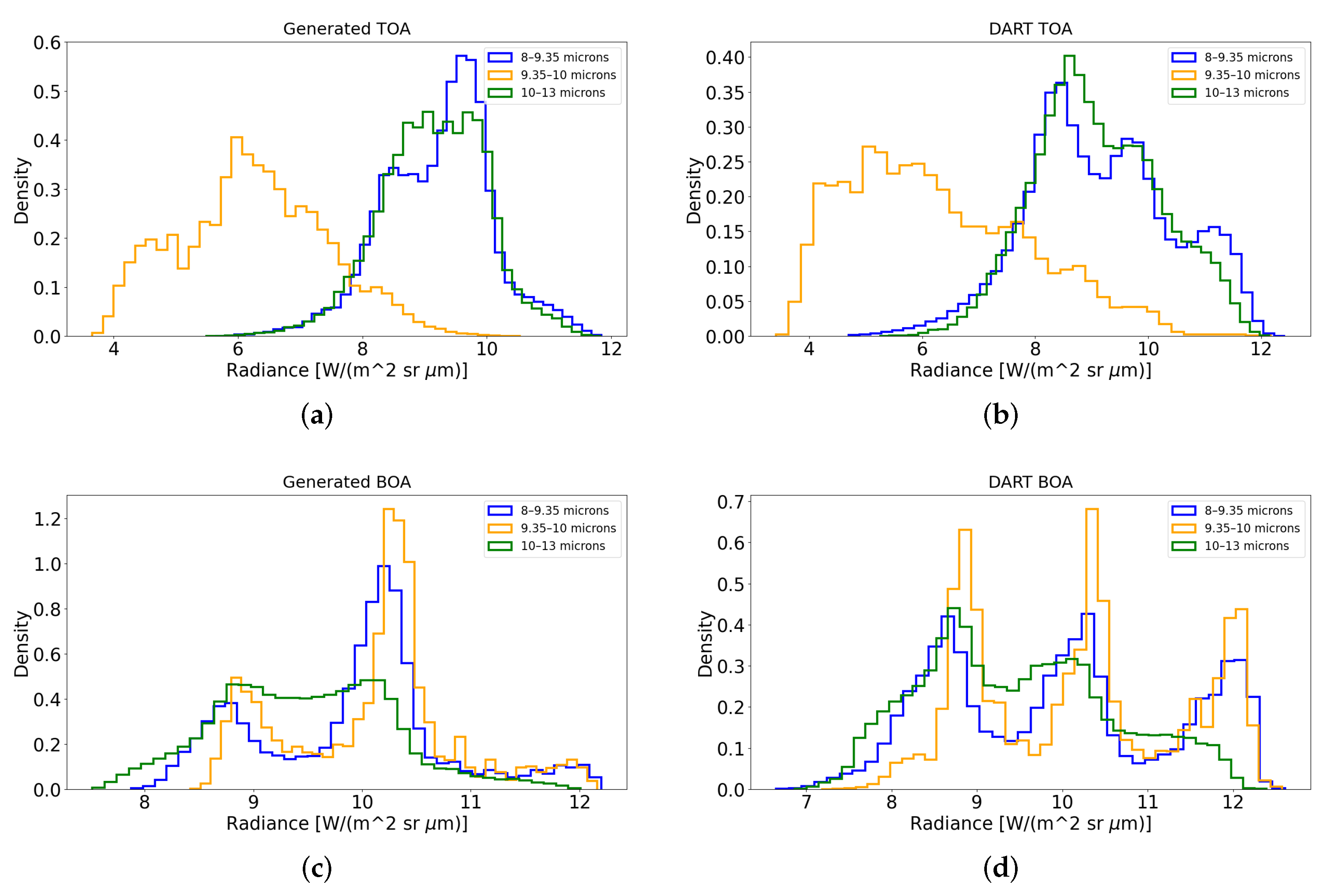
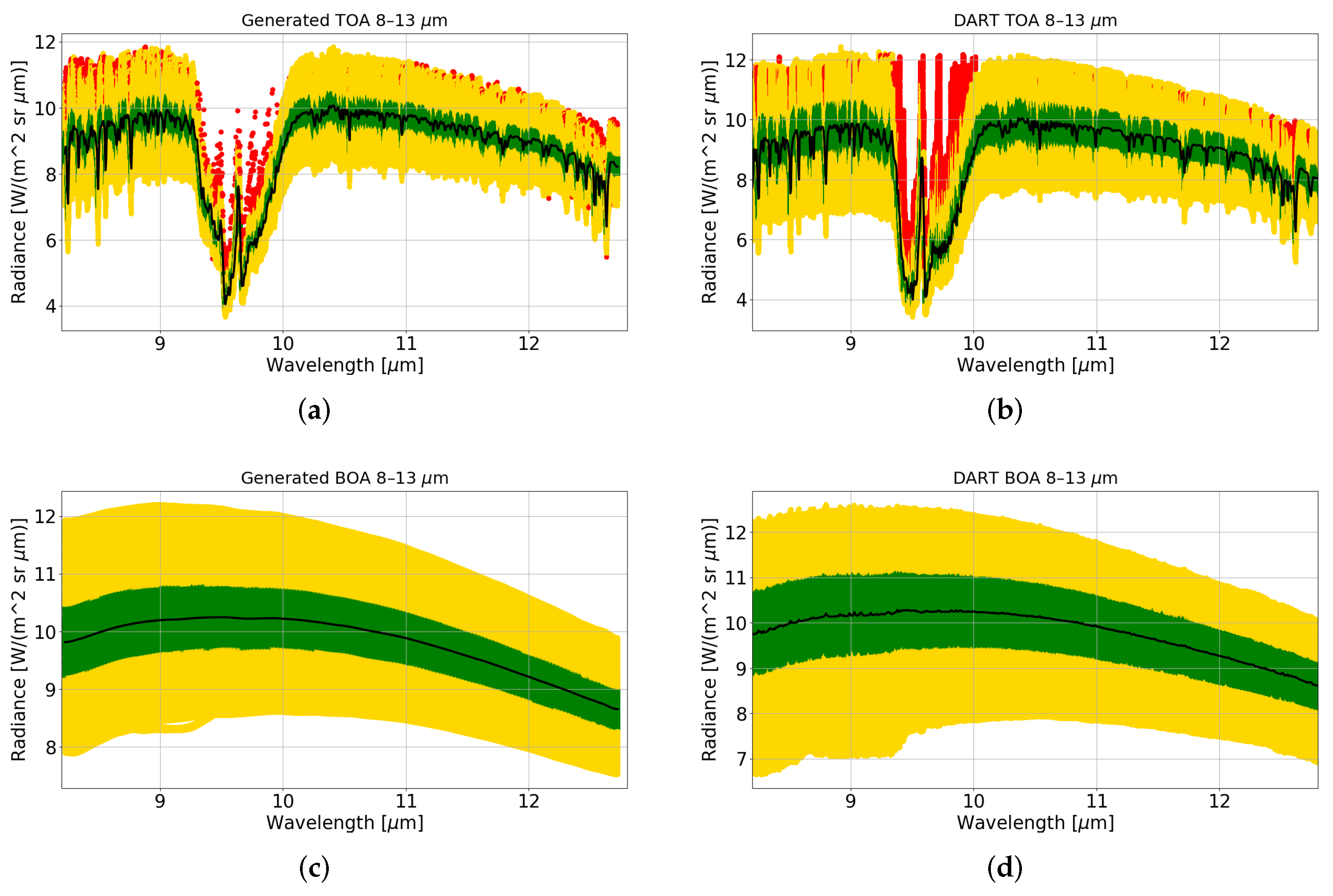
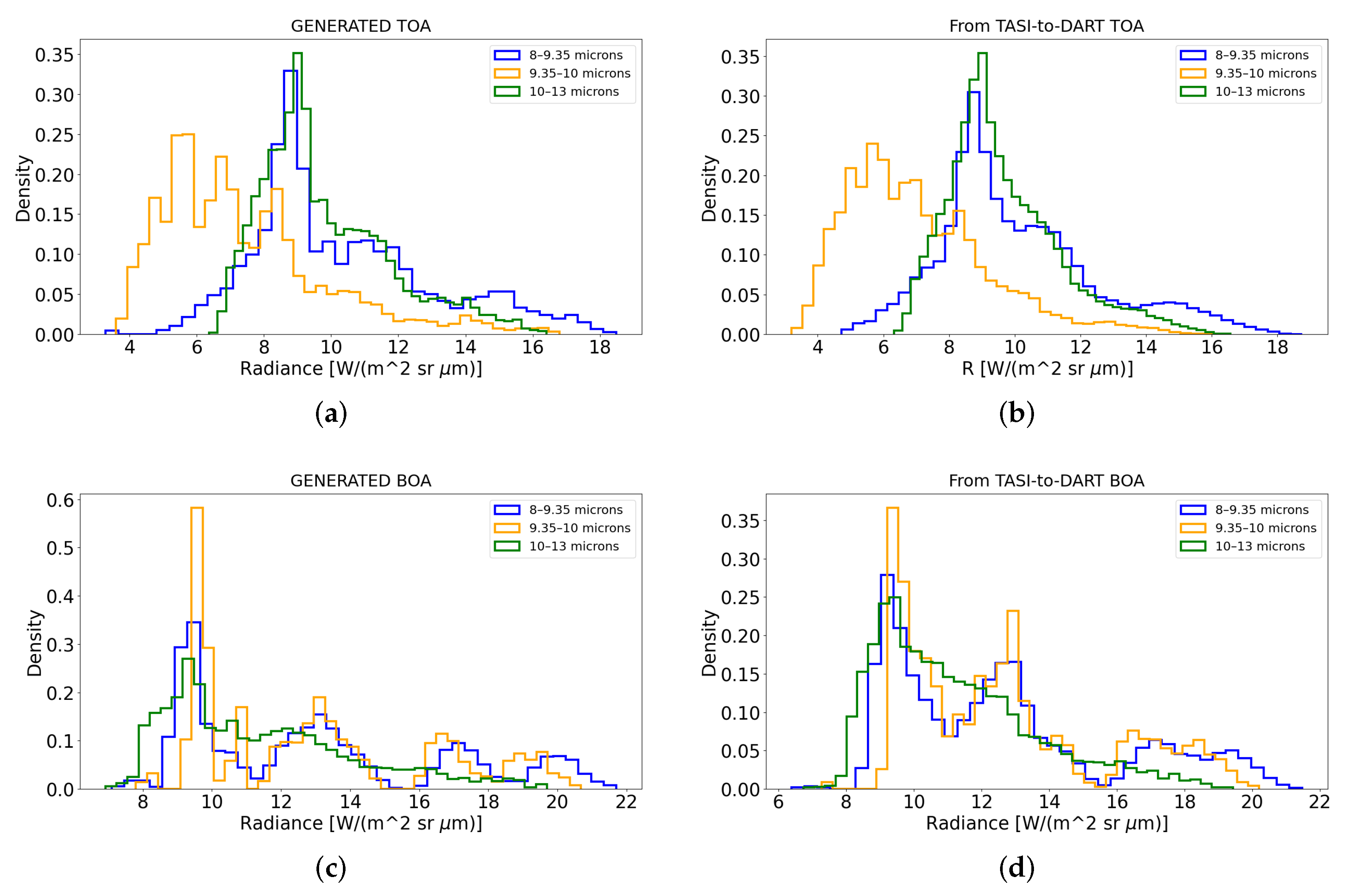
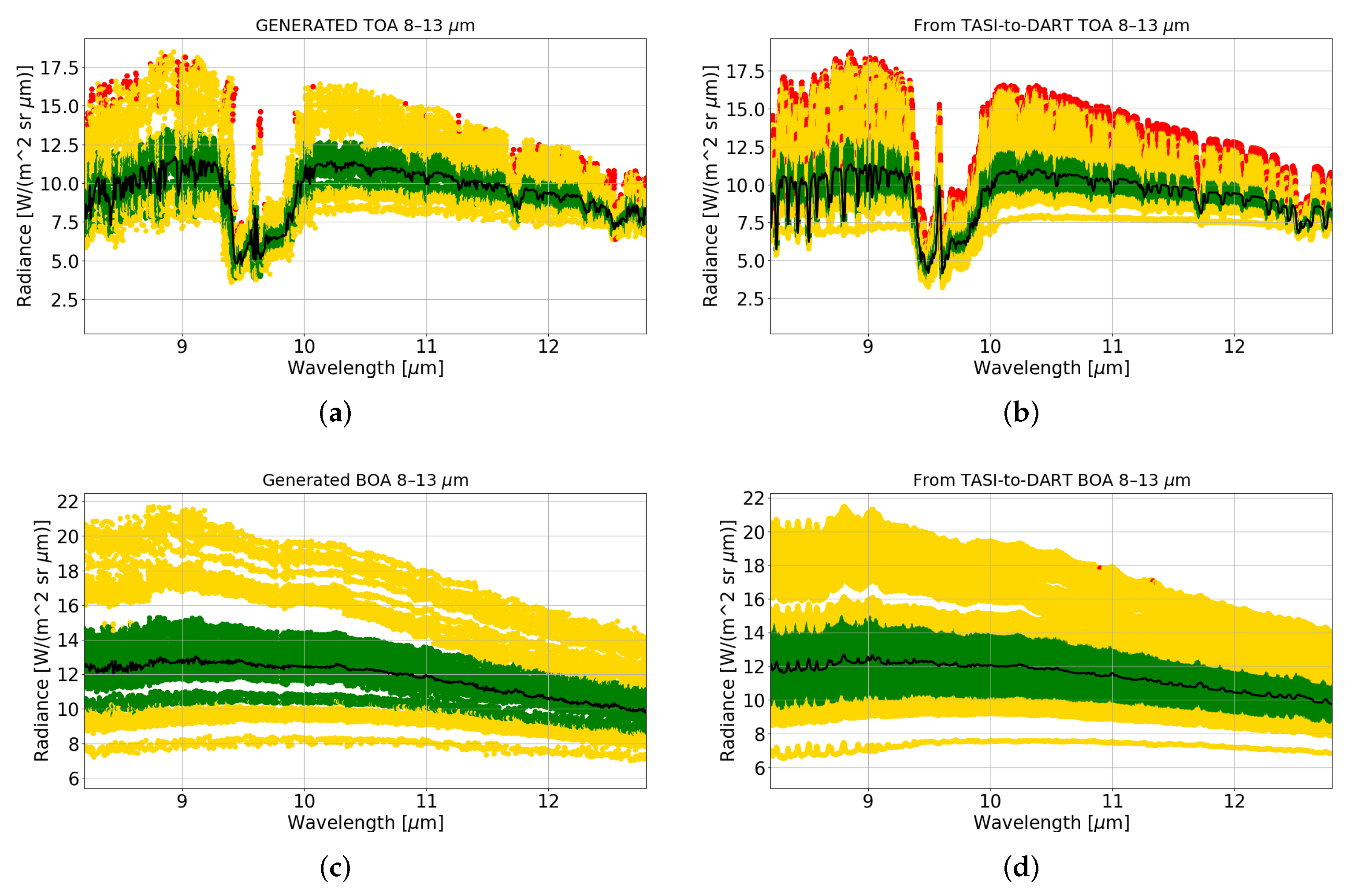
3.1. Assessment of Augmented Dataset vs. Original
3.2. Assessment of TIR Retrievals
Testing the Deep Learning Forward/Reverse Techniques
- 1.
- The use of generated signatures only: Both the training and the test datasets belong to the augmented dataset. No signatures from physically-based FM are included here. In case of instability in data generation, unphysical results can be found.
- 2.
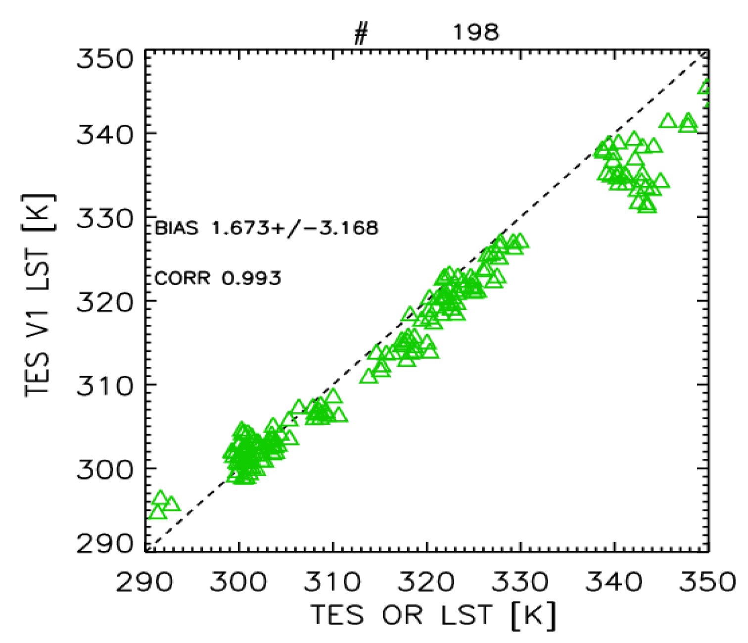
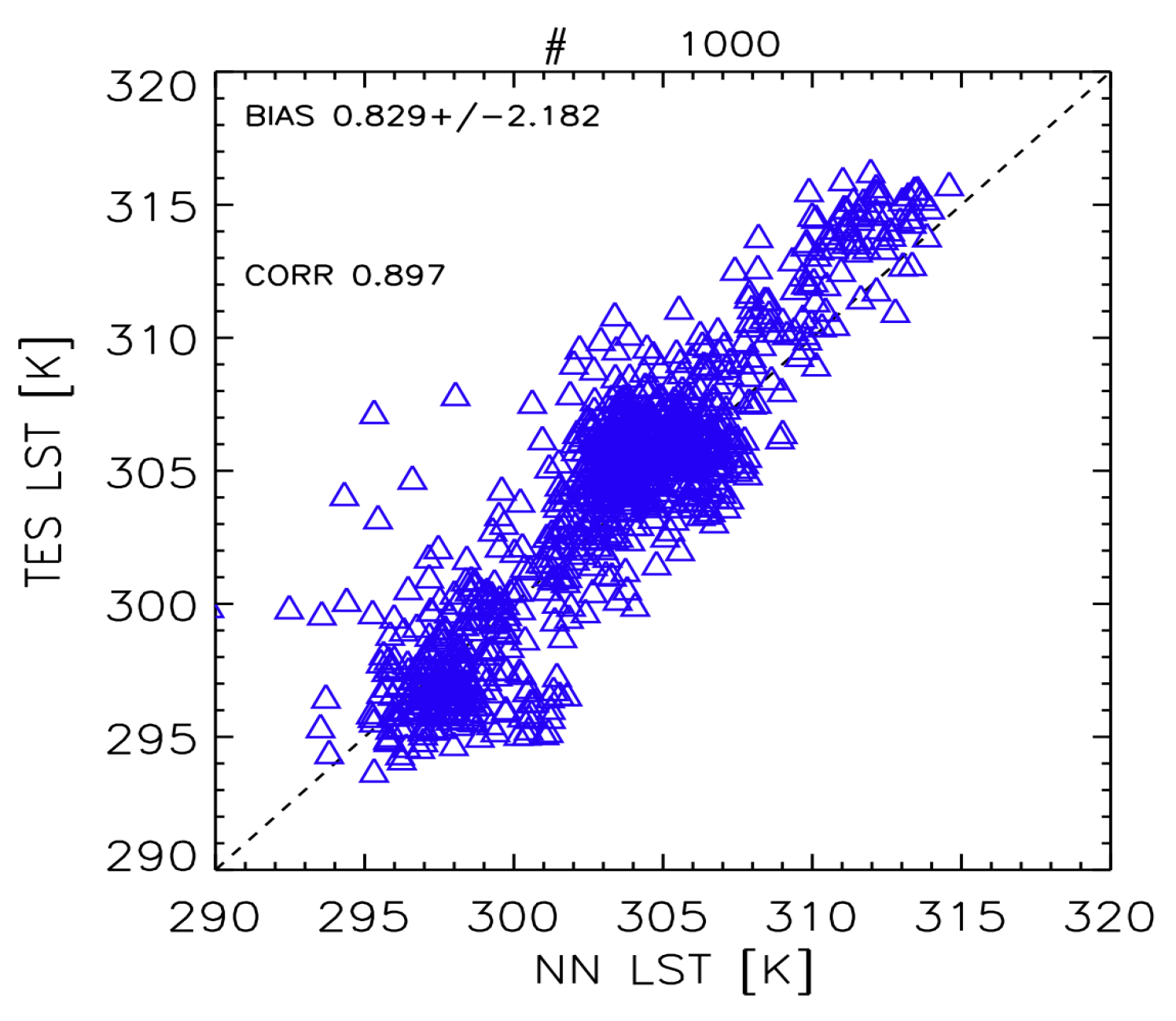
- The differences in training and test dataset: The NN is trained using signatures generated from DART. The GANDART spectra preserve the features of the original dataset (e.g., wheat emissivity and LST from about 295 K to about 320 K). The TASI2DART dataset, used as a test dataset, is generated from TASI data acquired over different vegetation (e.g., maize, rice) and ground surfaces with temperatures up to 350 K. Then, the training dataset does not fully cover the scenarios of the test dataset (e.g., high LST values, certain type of vegetation) and the NN tends to extrapolate the results.
4. Discussion
5. Conclusions
Author Contributions
Funding
Institutional Review Board Statement
Informed Consent Statement
Data Availability Statement
Conflicts of Interest
Abbreviations
| AE | AutoEncoders |
| ANN | Artificial Neural Network |
| ATSR | Along Track Scanning Radiometer simulations |
| BB | Broad Band |
| BBCH | Biologische Bundesanstalt, Bundessortenamt and CHemical industry |
| BOA | Bottom of the Atmosphere |
| BT | Brightness Temperature |
| DART | Discrete Anisotropic Radiative Transfer |
| DLIM | Deep Learning Inversion model |
| EDA | Exploratory Data Analysys |
| ECMWF | European Centre for Medium-range Weather Forecasts |
| ESA | European Space Agency |
| FM | Forward Model |
| FORUM | Far-Infrared-Outgoing Radiation Understanding and Monitoring |
| FOV | Field of View |
| GANs | Generative Adversarial Nets |
| GSW | Generalized Split Window |
| IASI | Infrared Atmospheric Sounding Interferometer |
| LAI | Leaf Area Index |
| LBL | Line-by-line |
| LSE | Land Surface Emissivity |
| LST | Land Surface Temperature |
| LSTM | Land Surface Temperature Mission |
| MAE | Mean Absolute Error |
| MMD | Maximum-Minimum Difference module |
| MRD | Mission Requirement Document |
| MSE | Mean Square Error |
| NEM | Normalized Emissivity Module |
| NN | Neural Network |
| NRT | Near Real Time |
| PGGANs | Progressive Growing of GANs |
| RMSE | Root Mean Square Error |
| RTM | Radiative Transfer Model |
| RTTOV | Radiative Transfer for TOVS |
| SRF | Spectral Response Function |
| TASI | Thermal Airborne Spectrographic Imager |
| TES | Temperature Emissivity Separation |
| TIR | Thermal Infra-Red |
| TOA | Top of the Atmosphere |
| VAE | Variational Autoencoder |
Appendix A

| Technology | Comments |
|---|---|
| GANDART | |
| Fully Connected GANs | First technology evaluated during the activity. |
| Results are too noisy to be consistent. | |
| The technology was dropped in favor of other models. | |
| Fully Convolutional GANs | This technology has been tried after the fully connected GANs, |
| it had reduced noise but still highly unreliable signature | |
| generation due to the unstructured latent space. | |
| ACGANs | Technology demonstrator for conditional generation. |
| Reliable and promising first results, | |
| however, the variability of the generated samples was too low. | |
| PGGANs | Very high quality for sample generation. |
| However, some artifacts are generated that disturb | |
| the retrieval process. | |
| Moreover, the unconditionality of the network | |
| reduce the potential for future uses. | |
| StyleGAN2 | Improved sample generation accuracy with respect to PGGANs. |
| Structured latent space generation. | |
| The results were produced using this technology. | |
| The exploration of the latent space needs to be refined. | |
| TASI2DART | |
| UNet + Custom | First technology demonstrator for the TASI to DART |
| generation process. | |
| Noisy results partially solved using a fully connected network. | |
| UNet + ENet | Technology improvement with respect to the previous model. |
| Completely solved the issue of noisy generated data, | |
| without the use of a fully connected network. | |
| Lightweight and fast to train model has been used. | |
| The results were produced using this technology. | |
| DLIM | |
| Convolutional Neural Network | First technology considered for inversion modeling. |
| At this stage of the project, the model input was the full signatures | |
| and not the convolved features. The technology was dropped | |
| when the input was changed to only the 5 convolved features. | |
| Deep Fully Connected | No particular problems with this technology, |
| but not outstanding results either. The technology was dropped | |
| in favor of a more promising technology (Autoencoders). | |
| Deep Autoencoders | Final technology selected for DLIM. Able to map data |
| distribution in a latent space useful to retrieve the outputs. |
References
- Eyre, J.R. A fast radiative transfer model for satellite sounding systems. In ECMWF Research Department Technical Memo; ECMWF: Reading, UK, 1991; Volume 176. [Google Scholar]
- Amato, U.; Masiello, G.; Serio, C.; Viggiano, M. The σ-IASI code for the calculation of infrared atmospheric radiance and its derivatives. Environ. Model. Softw. 2002, 17, 651–667. [Google Scholar] [CrossRef]
- Berger, K.; Rivera Caicedo, J.P.; Martino, L.; Wocher, M.; Hank, T.; Verrelst, J. A Survey of Active Learning for Quantifying Vegetation Traits from Terrestrial Earth Observation Data. Remote Sens. 2021, 13, 287. [Google Scholar] [CrossRef]
- Samarin, M.; Zweifel, L.; Roth, V.; Alewell, C. Identifying Soil Erosion Processes in Alpine Grasslands on Aerial Imagery with a U-Net Convolutional Neural Network. Remote Sens. 2020, 12, 4149. [Google Scholar] [CrossRef]
- Nemni, E.; Bullock, J.; Belabbes, S.; Bromley, L. Fully Convolutional Neural Network for Rapid Flood Segmentation in Synthetic Aperture Radar Imagery. Remote Sens. 2020, 12, 2532. [Google Scholar] [CrossRef]
- Goodfellow, I.J.; Pouget-Abadie, J.; Mirza, M.; Xu, B.; Warde-Farley, D.; Ozair, S.; Courville, A.; Bengio, Y. Generative Adversarial Nets. Available online: https://arxiv.org/abs/1406.2661 (accessed on 24 November 2021).
- Hinton, G.E.; Salakhutdinov, R.R. Reducing the Dimensionality of Data with Neural Networks. Science 2006, 313, 504–507. [Google Scholar] [CrossRef] [PubMed] [Green Version]
- Theis, L.; Shi, W.; Cunningham, A.; Huszár, F. Lossy Image Compression with Compressive Autoencoders. Available online: https://arxiv.org/abs/1703.00395 (accessed on 25 November 2021).
- Ronneberger, O.; Fischer, P.; Brox, T. U-Net: Convolutional Networks for Biomedical Image Segmentation. Available online: https://arxiv.org/abs/1505.04597 (accessed on 25 November 2021).
- Kingma, D.P.; Welling, M. Auto-Encoding Variational Bayes. Available online: https://arxiv.org/abs/1312.6114 (accessed on 25 November 2021).
- Koetz, B.; Bastiaanssen, W.; Berger, M.; Defourney, P.; Bello, U.D.; Drusch, M.; Drinkwater, M.; Duca, R.; Fernandez, V.; Ghent, D.; et al. High Spatio-Temporal Resolution Land Surface Temperature Mission—A Copernicus Candidate Mission in Support of Agricultural Monitoring. In Proceedings of the IGARSS 2018–2018 IEEE International Geoscience and Remote Sensing Symposium, Valencia, Spain, 22–27 July 2018; pp. 8160–8162. [Google Scholar] [CrossRef]
- Plans for a New Wave of European Sentinel Satellites, ESA. 2020. Available online: https://futureearth.org/wp-content/uploads/2020/01/issuebrief_04_03.pdf (accessed on 25 August 2021).
- ESA Earth and Mission Science Division. Copernicus High Spatio-Temporal Resolution Land Surface Temperature Mission: Mission Requirements Document. Issue Date 14/05/2021 Ref ESA-EOPSM-HSTR-MRD-3276. Available online: https://esamultimedia.esa.int/docs/EarthObservation/Copernicus_LSTM_MRD_v3.0_Issued_20210514.pdf (accessed on 24 November 2021).
- Gastellu–Etchegorry, J.P.; Lauret, N.; Yin, T.G.; Landier, L.; Kallel, A.; Malenovsky, Z.; Al Bitar, A.; Aval, J.; Benhmida, S.; Qi, J.B.; et al. DART: Recent advances in remote sensing data modeling with atmosphere, polarization, and chlorophyll fluorescence. IEEE J. Sel. Top. Appl. Earth Obs. Remote Sens. 2017, 10, 2640–2649. [Google Scholar] [CrossRef]
- Fournier, C.; Andrieu, B.; Ljutovac, S.; Saint-Jean, S. ADEL-wheat: A 3D architectural model of wheat development. In Plant Growth Modeling and Applications; Hu, B.-G., Jaeger, M., Eds.; Tsinghua University Press: Beijing, China, 2003; pp. 54–63. [Google Scholar]
- Abichou, M.; Fournier, C.; Dornbusch, T.; Chambon, C.; Baccar, R.; Bertheloot, J.; Vidal, T.; Robert, C.; David, G.; Andrieu, B. Re-parametrisation of Adel-wheat allows reducing the experimental effort to simulate the 3D development of winter wheat. Risto Sievänen and Eero Nikinmaa and Christophe Godin and Anna Lintunen and Pekka Nygren. In Proceedings of the 7th International Conference on Functional-Structural Plant Models, Saariselka, Finland, 9–14 June 2013; pp. 304–306. [Google Scholar]
- Abichou, M. Modélisation de L’architecture 4D du blé: Identification des Patterns Dans la Morphologie, la Sénescence et le Positionnement Spatial des Organes Dans une Large Gamme de Situations de Croissance. PhD University Paris-Saclay, AgroParisTech. 2016. Available online: https://www.researchgate.net/profile/Abichou_Mariem (accessed on 2 December 2021).
- Abichou, M.; Fournier, C.; Dornbusch, T.; Chambon, C.; Solan, B.d.; Gouache, D.; Andrieu, B. Parameterising wheat leaf and tiller dynamics for faithful reconstruction of wheat plants by structural plant models. Field Crop. Res. 2018, 218, 213–230. [Google Scholar] [CrossRef]
- Rascher, U.; Sobrino, J.A.; Skokovic, D.; Hanus, J.; Siegmann, B. SurfSense Technical Assistance for Airborne and Ground Measurements during the High Spatio-Temporal Resolution Land Surface Temperature Experiment Final Report. Unpublished work. 2019. [Google Scholar]
- ITRES TASI Instrument Manual; Document ID: 360025-03; ITRES Research Limited: Calgary, AB, Canada, 2008.
- Delderfield, J.; Llewellyn-Jones, D.T.; Bernard, R.; de Javel, Y.; Williamson, E.J.; Mason, I.; Pick, D.R.; Barton, I.J. The Along Track Scanning Radiometer (ATSR) for ERS-1. Proc. SPIE 1986, 589, 114–120. [Google Scholar]
- Casadio, S.; Castelli, E.; Papandrea, E.; Dinelli, B.M.; Pisacane, G.; Bojkov, B. Total column water vapour from along track scanning radiometer series using thermal infrared dual view ocean cloud free measurements: The Advanced Infra-Red Water Vapour Estimator (AIRWAVE) algorithm. Remote Sens. Environ. 2016, 172, 1–14. [Google Scholar] [CrossRef]
- Castelli, E.; Papandrea, E.; Di Roma, A.; Dinelli, B.M.; Casadio, S.; Bojkov, B. The Advanced Infra-RedWAter Vapour Estimator (AIRWAVE) version 2: Algorithm evolution, dataset description and performance improvements. Atmos. Meas. Tech. 2019, 12, 371–388. [Google Scholar] [CrossRef] [Green Version]
- Silvestro, P.C.; Casa, R.; Hanus, J.; Koetz, B.; Rascher, U.; Schuettemeyer, D.; Siegmann, B.; Skokovic, D.; Sobrino, J.; Tudoroiu, M. Synergistic Use of Multispectral Data and Crop Growth Modelling for Spatial and Temporal Evapotranspiration Estimations. Remote Sens. 2021, 13, 2138. [Google Scholar] [CrossRef]
- Remedios, J.J.; Leigh, R.J.; Waterfall, A.M.; Moore, D.P.; Sembhi, H.; Parkes, I.; Greenhough, J.; Chipperfield, M.P.; Hauglustaine, D. MIPAS reference atmospheres and comparisons to V4.61/V4.62 MIPAS level 2 geophysical data sets. Atmos. Chem. Phys. Discuss. 2007, 7, 9973–10017. [Google Scholar]
- Karras, T.; Aila, T.; Laine, S.; Lehtinen, J. Progressive Growing of Gans for Improved Quality, Stability, Variation. Available online: https://arxiv.org/abs/1710.10196 (accessed on 24 November 2021).
- He, K.; Zhang, X.; Ren, S.; Sun, J. Deep Residual Learning for Image Recognition. Available online: https://arxiv.org/abs/1512.03385 (accessed on 24 November 2021).
- Karras, T.; Laine, S.; Timo, A. A Style-Based Generator Architecture for Generative Adversarial Networks. Available online: https://arxiv.org/abs/1812.04948 (accessed on 24 November 2021).
- Ballard, D.H. Modular Learning in Neural Networks. In Proceedings of the Sixth National Conference on Artificial Intelligence (AAAI-87), Seattle, WA, USA, 13–17 July 1987; AAAI Press: Palo Alto, CA, USA, 1987; Volume 1, pp. 279–284. Available online: https://www.aaai.org/Papers/AAAI/1987/AAAI87-050.pdf (accessed on 22 September 2020).
- Tan, M.; Le, Q.V. Efficient Net: Rethinking Model Scaling for Convolutional Neural Networks. In Proceedings of the 36th International Conference on Machine Learning, PMLR 97:6105-6114, Long Beach, CA, USA, 9–15 June 2019; Available online: https://arxiv.org/pdf/1905.11946.pdf (accessed on 31 May 2019).
- Deng, J.; Dong, W.; Socher, R.; Li, L.J.; Li, K.; Li, F.-F. Image Net: A Large-Scale Hierarchical Image Database. In Proceedings of the 2009 IEEE Conference on Computer Vision and Pattern Recognition, Miami, FL, USA, 20–25 June 2009; pp. 248–255. [Google Scholar] [CrossRef] [Green Version]
- Zeiler, M.D.; Krishnaan, D.; Taylor, G.W.; Fergus, G. Deconvolutional networks. In Proceedings of the CVPR, IEEE Computer Society Conference on Computer Vision and Pattern Recognition, San Francisco, CA, USA, 13–18 June 2010. [Google Scholar]
- Rumelhart, D.E.; Hinton, G.E.; Williams, R.J. Learning representations by back-propagating errors. Nature 1986, 323, 533–536. [Google Scholar] [CrossRef]
- Gillespie, A.R.; Rokugawa, S.; Hook, S.J.; Matsunaga, T.; Kahle, A.B. ASTER ATBD, Temperature/Emissivity Separation Algorithm Theoretical Basis Document, Version 2.4, Prepared under NASA Contract NAS5-31372. 22 March 1999. Available online: https://unit.aist.go.jp/igg/rs-rg/ASTERSciWeb_AIST/en/documnts/pdf/2b0304.pdf (accessed on 2 December 2021).
- Wan, Z.; Dozier, J. A generalized split-window algorithm for retrieving land-surface temperature from space. IEEE Trans. Geosci. Remote Sens. 1996, 34, 892–905. [Google Scholar]
- Castelli, E.; Papandrea, E.; Valeri, M.; Greco, F.P.; Ventrucci, M.; Casadio, S.; Dinelli, B.M. ITCZ trend analysis via Geodesic P-spline smoothing of the AIRWAVE TCWV and cloud frequency datasets. Atmos. Res. 2018, 214, 228–238. [Google Scholar] [CrossRef] [Green Version]
- Diederik, P.K.; Adam, J.B. A Method for Stochastic Optimization. In Proceedings of the 3rd International Conference for Learning Representations, San Diego, CA, USA, 7–9 May 2015. [Google Scholar]
- Sobrino, J.A.; Del Frate, F.; Drusch, M.; Jimenez-Munoz, J.C.; Manunta, P.; Regan, A. Review of thermal infrared applications and requirements for future high-resolution sensors. IEEE Trans. Geosci. Remote Sens. 2016, 54, 2963–2972. [Google Scholar] [CrossRef]
- Forum. Available online: https://www.forum-ee9.eu (accessed on 27 August 2021).
- Palchetti, L.; Brindley, H.; Bantges, R.; Buehler, S.A.; Camy-Peyret, C.; Carli, B.; Cortesi, U.; Del Bianco, S.; Di Natale, G.; Dinelli, B.M.; et al. FORUM: Unique far-infrared satellite observations to better understand how Earth radiates energy to space. Bull. Am. Meteor. Soc. 2020, 101, E2030–E2046. [Google Scholar] [CrossRef]
- IASI. Available online: https://www.eumetsat.int/iasi (accessed on 27 August 2021).


| Overall RMSE [K] | Overall MAE [K] | Overall MSE [K] | TOA MSE [K] | |
|---|---|---|---|---|
| Validation | 0.189 | 0.076 | 0.0357 | 0.001 |
| Training | 0.251 | 0.124 | 0.0632 | NA |
| Spectral Region [µm] | TOA [W/(m sr µm)] | BOA [W/(m sr µm)] | RATIO BOA/TOA | |||
|---|---|---|---|---|---|---|
| DART | GANDART | DART | GANDART | DART | GANDART | |
| 8–9.35 | 9.15 ± 1.30 | 9.21 ± 0.86 | 9.92 ± 1.36 | 9.91 ± 0.87 | 1.08 ± 0.3 | 1.08 ± 0.19 |
| 9.35–10 | 6.28 ± 1.58 | 6.25 ± 1.71 | 10.18 ± 1.22 | 10.09 ± 0.79 | 1.62 ± 0.60 | 1.62 ± 0.43 |
| 10–13 | 9.10 ± 1.10 | 9.15 ± 0.84 | 9.48 ± 1.11 | 9.47 ± 0.79 | 1.04 ± 0.25 | 1.04 ± 0.18 |
| Spectral Region [µm] | TOA [W/(m sr µm)] | BOA [W/(m sr µm)] | RATIO BOA/TOA | |||
|---|---|---|---|---|---|---|
| TASI-to-D. | TASI2DART | TASI-to-D. | TASI2DART | TASI-to-D. | TASI2DART | |
| 8–9.35 | 10.09 ± 2.45 | 10.32 ± 2.7 | 12.61 ± 3.30 | 12.99 ± 3.72 | 1.25 ± 0.63 | 1.25 ± 0.69 |
| 9.35–10 | 7.01 ± 2.14 | 7.38 ± 2.45 | 12.60 ± 2.93 | 12.97 ± 3.34 | 1.80 ± 0.97 | 1.76 ± 1.03 |
| 10–13 | 9.66 ± 1.72 | 9.82 ± 1.94 | 11.24 ± 2.35 | 11.40 ± 2.68 | 1.16 ± 0.45 | 1.16 ± 0.50 |
Publisher’s Note: MDPI stays neutral with regard to jurisdictional claims in published maps and institutional affiliations. |
© 2021 by the authors. Licensee MDPI, Basel, Switzerland. This article is an open access article distributed under the terms and conditions of the Creative Commons Attribution (CC BY) license (https://creativecommons.org/licenses/by/4.0/).
Share and Cite
Castelli, E.; Papandrea, E.; Di Roma, A.; Bloise, I.; Varile, M.; Tabani, H.; Gastellu-Etchegorry, J.-P.; Feruglio, L. Deep Learning Application to Surface Properties Retrieval Using TIR Measurements: A Fast Forward/Reverse Scheme to Deal with Big Data Analysis from New Satellite Generations. Remote Sens. 2021, 13, 5003. https://0-doi-org.brum.beds.ac.uk/10.3390/rs13245003
Castelli E, Papandrea E, Di Roma A, Bloise I, Varile M, Tabani H, Gastellu-Etchegorry J-P, Feruglio L. Deep Learning Application to Surface Properties Retrieval Using TIR Measurements: A Fast Forward/Reverse Scheme to Deal with Big Data Analysis from New Satellite Generations. Remote Sensing. 2021; 13(24):5003. https://0-doi-org.brum.beds.ac.uk/10.3390/rs13245003
Chicago/Turabian StyleCastelli, Elisa, Enzo Papandrea, Alessio Di Roma, Ilaria Bloise, Mattia Varile, Hamid Tabani, Jean-Philippe Gastellu-Etchegorry, and Lorenzo Feruglio. 2021. "Deep Learning Application to Surface Properties Retrieval Using TIR Measurements: A Fast Forward/Reverse Scheme to Deal with Big Data Analysis from New Satellite Generations" Remote Sensing 13, no. 24: 5003. https://0-doi-org.brum.beds.ac.uk/10.3390/rs13245003