
A Remote Sensing Image Destriping Model Based on Low-Rank and Directional Sparse Constraint
by
 , and
, and
Xiaobin Wu
1,2,3 ,
,
Hongsong Qu
1,2,3,
Liangliang Zheng
1,2,3,*,
Tan Gao
1,2,3 and
Ziyu Zhang
1,2,3 1
Changchun Institute of Optics, Fine Mechanics and Physics, Chinese Academy of Sciences, Changchun 130033, China
2
University of Chinese Academy of Sciences, Bijing 100039, China
3
Key Laboratory of Space-Based Dynamic & Rapid Optical Imaging Technology, Chinese Academy of Sciences, Changchun 130033, China
*
Author to whom correspondence should be addressed.
Remote Sens. 2021, 13(24), 5126; https://0-doi-org.brum.beds.ac.uk/10.3390/rs13245126
Submission received: 19 November 2021
/
Revised: 8 December 2021
/
Accepted: 10 December 2021
/
Published: 17 December 2021
(This article belongs to the Special Issue Remote Sensing Image Denoising, Restoration and Reconstruction)
Abstract
:Stripe noise is a common condition that has a considerable impact on the quality of the images. Therefore, stripe noise removal (destriping) is a tremendously important step in image processing. Since the existing destriping models cause different degrees of ripple effects, in this paper a new model, based on total variation (TV) regularization, global low rank and directional sparsity constraints, is proposed for the removal of vertical stripes. TV regularization is used to preserve details, and the global low rank and directional sparsity are used to constrain stripe noise. The directional and structural characteristics of stripe noise are fully utilized to achieve a better removal effect. Moreover, we designed an alternating minimization scheme to obtain the optimal solution. Simulation and actual experimental data show that the proposed model has strong robustness and is superior to existing competitive destriping models, both subjectively and objectively.
1. Introduction
The non-uniform photoresponse of image detectors causes stripe noise with distinct directional and structural features. It will reduce the subjective quality of images and limit their subsequent application in many fields. Therefore, the purpose of our research is to estimate potential prior components to separate the clear image from the degraded image.
In the past few decades, many researchers have carried out related work, which can be roughly divided into two categories: one relies on radiometric calibration and the other is based on image processing. The former establishes a mathematical model between spectral radiation and the response of the image sensor with radiation sources of varying degree generated by the integrating sphere. The latter analyzes the causes of stripe noise and establishes a degradation model to achieve destriping. Since there are many limitations of the method based on calibration, this paper adopts an idea, based on image processing, for removing stripe noise. At present, there are three kinds of destriping methods based on image processing: methods based on filtering, methods based on statistical theory and methods based on optimization.
The first method filters the degraded image in the transform domain by designing different filters [1,2,3,4,5,6,7,8]. In [3], wavelet analysis was used to remove stripe noise from satellite imagery. In [4], an FIR filter was proposed to filter the image in the frequency domain. In addition, Münch et al. [6] proposed a combination filter that uses wavelet decomposition to improve filtering accuracy to separate stripes. This method is simple in operation and fast in processing, but it can not remove non-periodic stripes completely.
The second method usually considers using the statistical characteristics of the sensors to remove stripe noise [9,10,11,12,13,14,15,16]. Histogram matching and moment matching are two typical methods. The former is usually matched with a histogram of the reference signal to remove the stripe noise. The latter generally assumes that each image sensor has the same standard deviation and mean value, then selects the ideal reference data, using moment matching to restore the image. In [9], histogram matching was used. Wegener et al. [10] introduced a process of calculating homogeneous regions before histogram matching. The author also used moment matching in [12]. In [14], local-least-squares fitting was considered for combination with histogram matching to restore the image. Limited by previous assumptions, the destriping effect of this method shows great variation, which indicates that the model has poor reliability and robustness.
In recent years, lots of models based on optimization [17,18,19,20,21,22,23,24,25,26,27] have been proposed that regard the destriping issue as an ill-posed inverse problem. To find the optimal solution, constructing a proper regularized model for the underlying prior information of the image is necessary. Therefore, this method focuses on finding potential prior information and corresponding regularization terms. In [17], the Huber–Markov variation model was proposed, firstly. In [18], the author proposed a complex single-term total variation model (UTV), which used stripes’ structure and direction characteristics to preserve image details. Chang et al. [22] adopted the idea of image decomposition, proposing the low-rank single image destriping (LRSID) model to estimate two priors simultaneously. Liu et al. [23] separated stripe noise from degraded images by considering global sparsity and local variational (GSLV) properties. In [24], the author used a regularized model that combines the total variation and global sparse (TVGS) constraint. In [27], a destriping model based on hybrid total variation and nonconvex low-rank (HTVLR) regularization was proposed to reduce the staircase effect caused by the TV model.
In general, the mentioned models can remove stripe noise in most cases, but they still have some drawbacks when dealing with different remote sensing images. For instance, in the low-rank constrained model proposed in [22], the structural and directional characteristics of the stripes are not fully utilized. In [23], the author only focuses on the stripe noise components in the degraded image, ignoring the properties of the underlying image information, which will destroy the smoothness of the restored image. The TVGS model proposed in [24] lacks a constraint term perpendicular to the stripe direction and may result in ripple effects. In [27], the HTVLR model could reduce the staircase effect caused by the TV model but could not maintain well its destriping performance when dealing with different stripes.
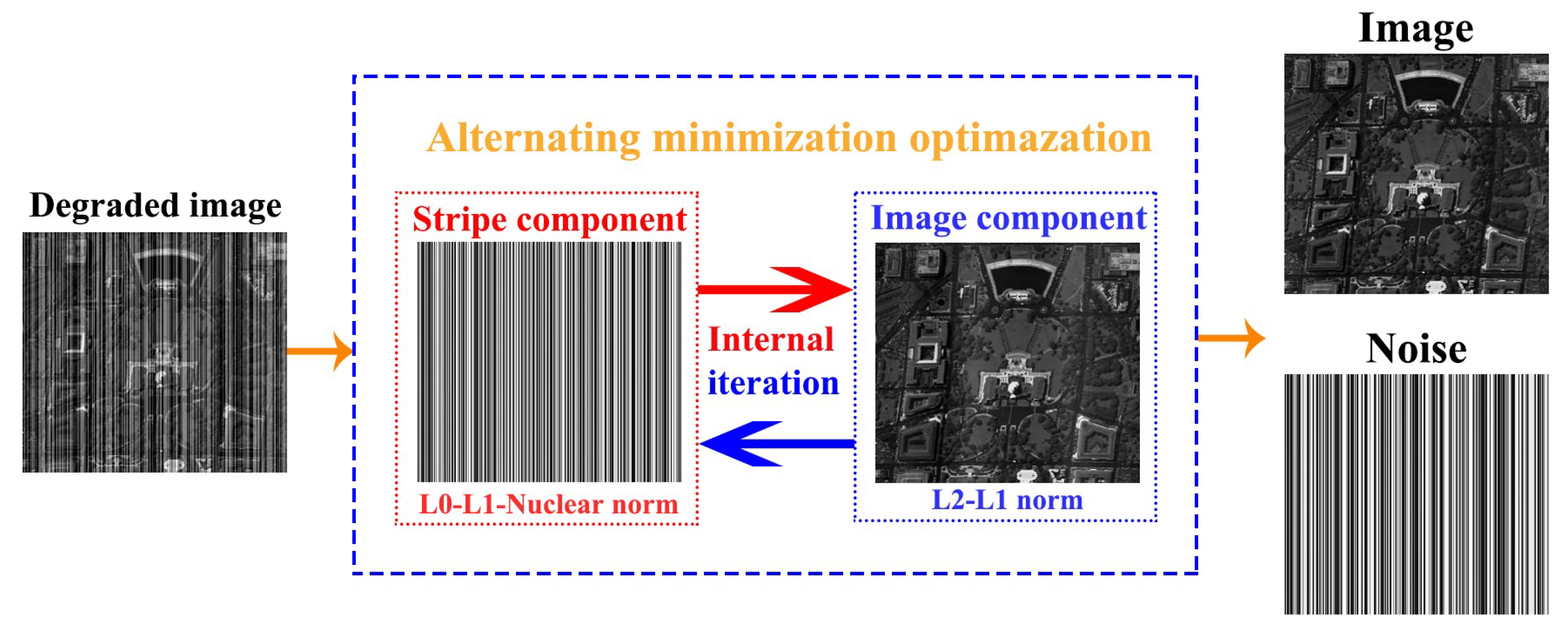
Focusing on the problems in the above methods, we apply image decomposition and propose a destriping model based on total variation and the low-rank direction sparse constraint. The TV model and low rank are taken to constrain the image prior and the stripe-noise prior globally. Different directional sparse constraints are adopted along and cross the stripe direction after taking full advantage of the structural and directional characteristics of the stripe noise. norm and norm are respectively taken to constrain the gradient matrix perpendicular to and along the stripe direction. Since the proposed model should estimate two factors simultaneously, an alternating minimization scheme is taken to find the optimal solution effectively. The specific framework of the solution is shown in Figure 1. Simulation and actual experimental data indicate that the proposed model shows better destriping performance compared with the five typical models. The main research work and innovative content of this article are summarized as follows:
- (a)
- Under the destriping model of image decomposition, a sparsity constraint, perpendicular to the stripes, is added to reduce the ripple effects of the output image.
- (b)
- After thoroughly analyzing the potential properties of stripe noise, we propose a regularization model combining low-rank and directional sparsity, enhancing the robustness of the stripe noise-removal model.
- (c)
- An alternate minimization scheme to the model is designed to estimate both potential priors in degraded images.
The subsequent contents are arranged as follows: the image-degradation model and the destriping model are introduced in Section 2. In Section 3, an alternating minimization algorithm is designed. The Section 4 verifies the destriping performance of the proposed model through many related experiments. In Section 5, the parameter value determination and future research are discussed. Section 6 is the conclusion of this paper.
2. Degradation Model and Proposed Model
Stripe noise, in remote sensing images, usually contains additive and multiplicative noise components [17]. Since multiplicative noise can be converted into additive noise through a logarithmic operation [15], stripe noise is usually treated as additive noise. Therefore, this type of image degradation model can be summarized as
where , and represent the original noisy image, clear image and stripe-noise image.
For convenience in the subsequent work, the formula (1) can be rewritten as follows:
where O, I and S represent the matrix forms of , and , respectively.
Both clear image, I, and stripe noise image, S, are the data we want to obtain from the degraded image, O, and the regularization can be considered to solve this typical ill-posed problem.
Taking into account the image decomposition model in [22], the constrained model for destriping can be expressed as:
where denotes the item representing the closeness between the degraded image and the sum of the clear image and the stripe noise. and are regularization terms, representing the information of the image prior and the stripe-noise prior. and are positive penalty parameters that are used to balance the constraint model. To obtain a better separation effect, it is necessary to select the appropriate regularization term and method.
2.1. The Regularization Term and Regularization Method of the Real Image
The most extensively used regularization methods in image processing are Tikhonov-like regularization [28] and TV-based regularization [29]. This paper adopts TV-based regularization to constrain the image prior due to its better performance in preserving image details.
For a two-dimensional image, TV constraint model can be expressed as:
we take the vertical and the horizontal direction as the y and x direction respectively in this paper; then, the regularization constraint of the clear image can be expressed as [30]:
where and represent the first derivative operator in the corresponding direction.
2.2. The Regularization Term and Regularization Method of the Stripe Noise Image
Singular value decomposition and eigenvalue decomposition can both be used to extract the matrix’s features. The difference is that eigenvalue decomposition only works with square matrices, but singular value decomposition works with any matrix. We can divide the original matrix into the product of three matrices using singular value decomposition. The second matrix is diagonal and its diagonal elements are the matrix’s singular values. We use the SVD function to perform singular value decomposition on the stripe image and plot its singular values in columns (see Figure 2). It can be found that the singular value quickly drops to 0 in the first few columns, which indicates that the stripe-noise prior can be regarded as a low-rank matrix [22]. In addition, the stripe noise image can also be viewed as a matrix with lots of zero elements. However, considering that the sparsity characteristic will disappear when stripes are too dense, we use the kernel norm to constrain the global low rank of the stripe noise. Therefore, this regularization term can be formulated as:
For stripe noise images, we assume that the direction of the stripes is the same as the y direction. The gradient matrix along the stripe direction is an obvious sparse matrix due to the sameness of intensity of each column, so this regularization term can be formulated as:
In addition, a constraint along the x-direction is needed to minimize the first derivative along the horizontal direction to ensure the continuity and smoothness of the clear images. According to formula (2), this constraint is added to the stripe-noise prior, and then this regularization term can be formulated as:
Based on the above analysis, the regularization term of the stripe-noise prior can be summarized as:
Finally, the destriping model in this paper can be summarized as:
where , , , and represent regularization parameters used to adjust the weight of each item to balance the model.
3. ADMM Optimization
The alternating direction multiplier method (ADMM) is usually considered to estimate the optimal value of this type of optimization problem. Therefore, we can decompose the above problem into two optimization sub-problems: the sub-problem of solving stripe-noise prior, S, and the sub-problem of solving image prior, I.
3.1. Image Prior Optimization Process
First, we fixed the stripe-noise prior, S, solving the image prior, I. The optimization model of I can be expressed as:
For convenience in the subsequent work, two auxiliary variables, and , are introduced to transform the above equation into the following form:
Subject to ,
Next, according to [31,32], the augmented Lagrangian equation, formula (12) can be expressed as:
where , and respectively represent the Lagrange multipliers and the positive penalty parameter. The problem of formula (13) can be considered to be divided into the following three sub-problems:
- (1)
- The M sub-problem can be summarized as
Soft threshold shrinkage is an effective way to solve this type of optimization problem [33]. Therefore, we can obtain the solution as follows:
where:
- (2)
- The N sub-problem can be summarized as
Same as the M sub-problem, we can get the solution as follows:
- (3)
- The I sub-problem can be described as
This equation is a typical quadratic optimization problem from which an optimal solution can be obtained. By differentiating the above equation, the formula (19) is converted to:
The two-dimensional Fourier transform is an effective method to solve the above problem [34]. Therefore, we update the image prior, I, as follows:
where
and represent the fast Fourier transform and the inverse fast Fourier transform.
Finally, we make the following update to the Lagrange multipliers and :
3.2. Stripe-Noise Prior Optimization Process
Second, we fix the image prior, I, solving the stripe-noise prior, S. The optimization model of S can be expressed as:
Similarly, three auxiliary variables, , , , are introduced to transform the above equation into the following constrained optimization problem:
where:
, , and are Lagrange multipliers and a positive penalty parameter. Similar to the formula (11), the problem of formula (25) can be considered to be divided into the following four sub-problems:
- (1)
- The W sub-problem can be summarized as
Singular value soft threshold shrinkage can be used to solve this type of optimization problem [35]:
where:
- (2)
- The H sub-problem can be summarized as
- (3)
- The K sub-problem can be summarized as
Soft threshold shrinkage can be used to solve this type of optimization problem:
- (4)
- The S sub-problem can be summarized as
Similar to the I sub-problem, the solution of this problem is:
where:
Finally, we will make the following update to the Lagrange multipliers , and :
The solution process of the model can be summarized in Algorithm 1:
| Algorithm 1: The proposed destriping model |
| Input: degraded image O, parameters , , , , , and . |
| 1: Initialize. |
| 2: for k= 1: N do |
| 3: update image prior: |
| 4: solve , and via(15), (18) and (21). |
| 5: update Lagrange multiplier and by (23) and (24). |
| 6: stripe component update: |
| 7: solve , , and via(30), (33), (36) and (38) |
| 8: update Lagrange multiplier , and by (40), (41), (42) |
| 9: end for |
| Output: image I and stripe S. |
4. Simulation and the Actual Destriping Experiment
In order to accurately evaluate the destriping performance of the proposed model, we carried out the simulation experiments and actual destriping experiments at the same time, assessing the destriping results both subjectively and objectively. Different indexes are chosen to evaluate the results, considering the differences between the simulation and actual destriping experiments.
Furthermore, five typical destriping methods, SLD [15], LRSID [22], GSLV [23], TVGS [24] and HTVLR [27], are selected as references to evaluate the proposed model. All methods have adjusted parameters to make the destriping effect suitable for comparison, except for LRSID, whose source code is published by the author on his website homepage. To compare the destriping effect intuitively, we make special remarks for the obvious differences.
4.1. Simulation Experiment
During the simulation experiments, we selected two typical image evaluation indicators, peak signal-to-noise ratio (PSNR) and structural similarity (SSIM) [38], to objectively evaluate the processing results. These indexes are as follows,
where and u are, respectively, the restored and the undegraded image, while n is the number of pixels.
where and denote the mean value of the two images, represents the covariance, and are constants that can be calculated in the following way: , , L represents the dynamic range of a pixel, and , .
There are two parts of the simulation experiments: simulation experiments under periodic and non-periodic stripe noise. The degree of image degradation is determined by r and I. Here, r denotes the proportion of the degraded region, and I represents the intensity of the added stripe noise. During the simulation experiments, we select noise ratios of 0.3, 0.5, 0.7 and 0.9, and intensities of 30, 50, 70 and 90. We treat these two parameters as an array for the convenience of expression. For example, (0.3, 50) represents the stripe ratio of 0.3 and the intensity of 50.
For periodic stripe noise, MODIS image band 32 and one typical region of the hyperspectral image of Washington DC Mall are selected to carry out the destriping experiment. The former is available from https://ladsweb.nascom.nasa.gov/, (accessed on 5 September 2021) and the latter can be downloaded from https://engineering.purdue.edu/~biehl/MultiSpec/ (accessed on 5 September 2021). Since the existing destriping methods all have a good removal effect in this case, we have only selected the results with noticeable differences for comparison. The partial destriping results of MODIS data are shown in Figure 3. The complete simulation data and results can be obtained from Table 1 and Table 2, and the best performance indexes are shown in bold.
According to the data in Table 1, SLD performs better when dealing with low-ratio and -intensity stripes; the proposed model shows a better destriping effect for the high-ratio and -intensity stripes. However, it can be found in Figure 3 that some residual stripes remain in the images restored by SLD, which shows a different result from Table 1. Furthermore, the results of the hyperspectral image show that the PSNR of SLD decreased rapidly with the noise ratio and intensity of (0.7, 90) and (0.9, 90), which indicates that it lost the original destriping effect. In terms of structural similarity (SSIM), the proposed model always performed best.
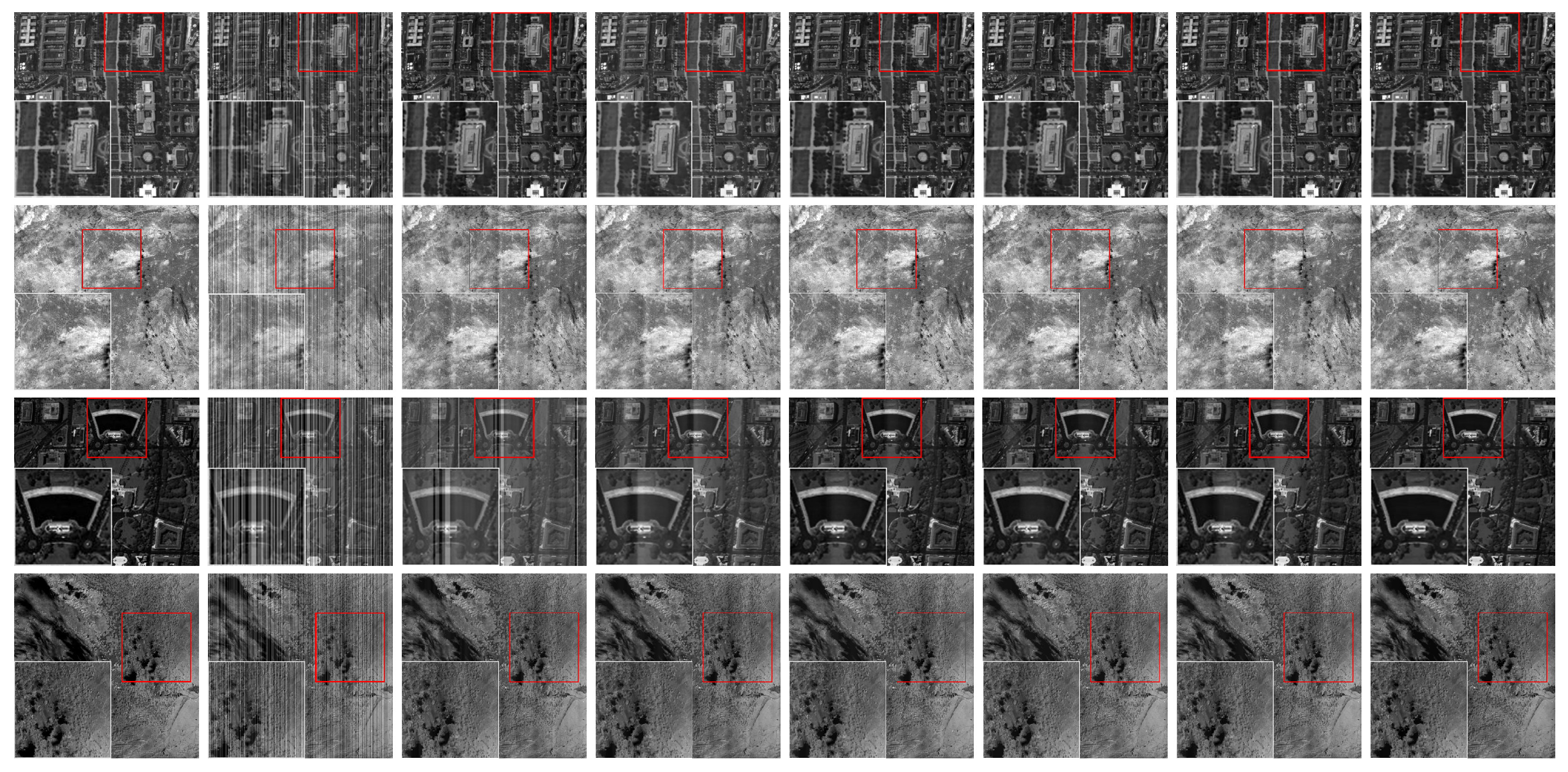
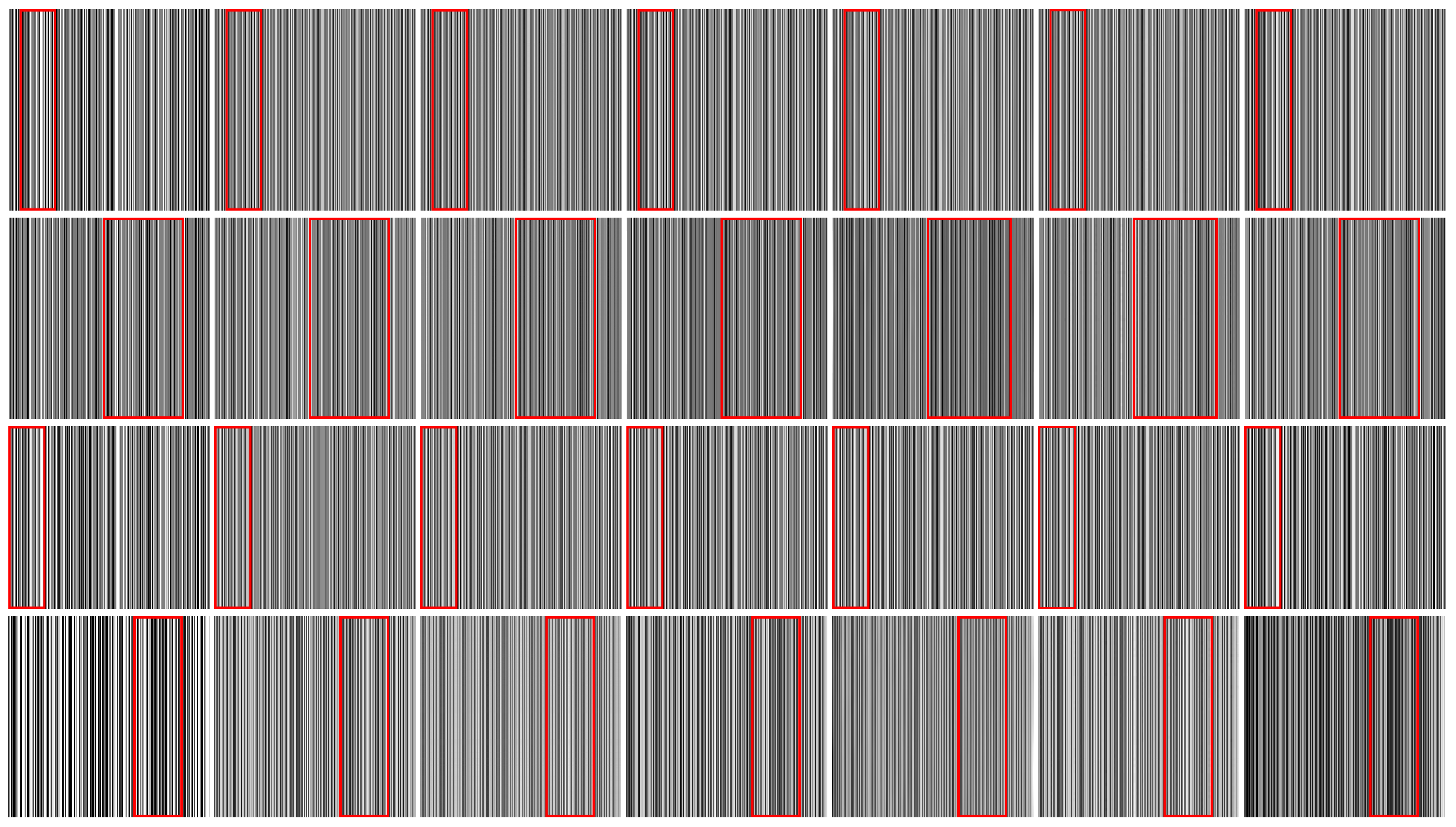
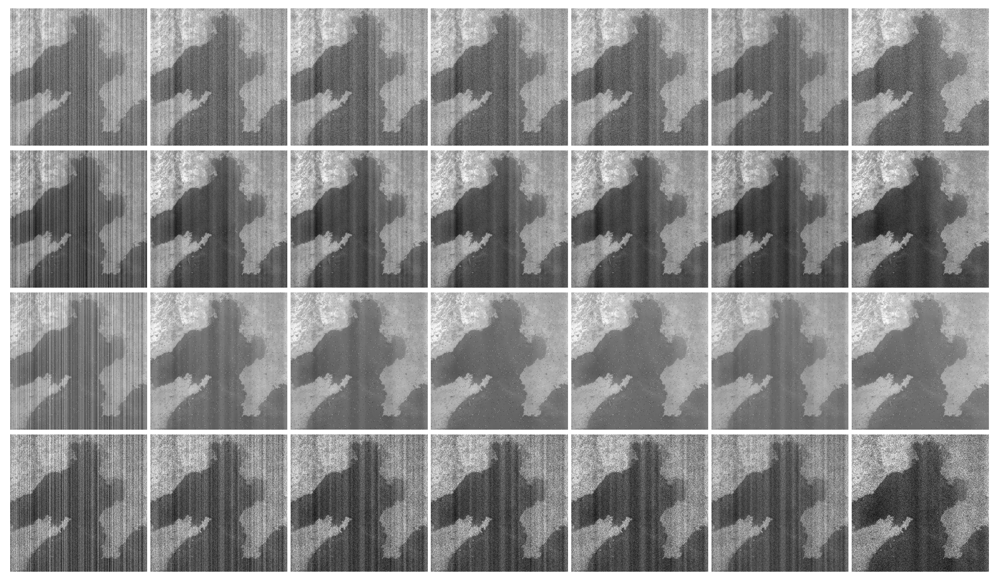
MODIS image band 20 and two typical regions of a hyperspectral image of the Washington DC Mall were chosen to carry out the destriping experiment with non-periodic stripes. The partial destriping results are shown in Figure 4 and Figure 5, with rectangular boxes in the images marking regions with obvious differences. Table 3 and Table 4 show PSNR and SSIM, respectively, with the best-performing indices highlighted in bold.
The objective evaluation indexes in Table 3 and Table 4 show that the TVGS performs better in some cases, but the proposed model shows stronger robustness over different noise intensities and ratios. HTVLR shows a good destriping effect at low intensity, but, as the noise gradually intensity increased, it was difficult for HTVLR to maintain good destriping performance. Subjectively, residual stripes and gray-scale loss are observed in the images restored by SLD, LRSID and HTVLR. TVGS and GSLV can remove the most noticeable stripes, but ripple effects influence the smoothness of the images. According to Figure 5, it can be found that the structure of the stripes is clear and there is no obvious image information. Additionally, the stripe image separated by the proposed model is much more similar to the added stripe when we focus on the region marked by the red rectangle.
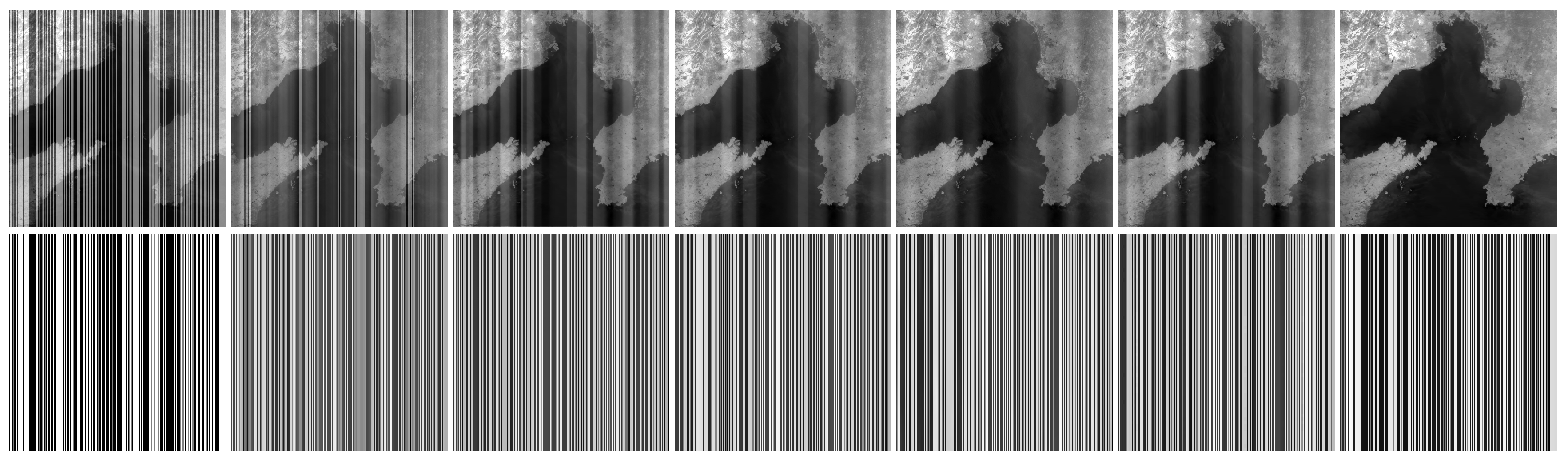
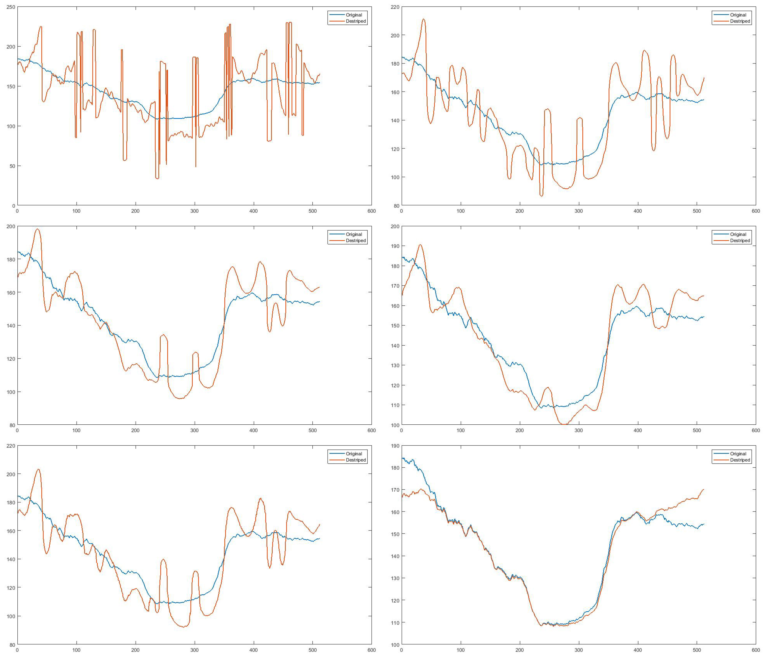
During the experiments, it was found that the existing methods showed worse removal effects when dealing with the stripes of high intensity and ratio, while the proposed model still maintained excellent performance. In this paper, related simulation experiments were carried out with MODIS data. We conducted experiments on a degraded image with a noise ratio of 0.9 and a noise intensity of 80, and the destriping results are shown in Figure 6. It shows that there are lots of residual stripes in the images restored by other methods. Additionally, we compared the column mean value of the restored images and the undegraded image; the results are shown in Figure 7. The curve in blue is the column mean value of the undegraded image, while the curve in orange represents that of restored images in Figure 6. We can find that the curve restored by the proposed model is generally consistent with the original curve.
Remote sensing images usually contain other random noise types that may affect the removal of stripe noise, so we conducted a simple simulation experiment on this situation. We added stripe noise with a ratio of 0.5 and an intensity of 50 to an image containing Gaussian noise, Poisson noise, salt-and-pepper noise and speckle noise to carry out the destriping experiment. The results are shown in Figure 8, from which we can find that the proposed model could still remove the stripes, but the removal effect was be affected by other random noise types. There is a certain degree of rippling effect in the processed results of the images containing Gaussian noise, Poisson noise and speckle noise, and there are some residual stripes in the image containing speckle noise.
We also tested the destriping performance on non-remote sensing images using data from the SIDD dataset, which can be found at https://paperswithcode.com/dataset/sidd, (accessed on 15 November 2021). Figure 9 shows these destriping results, which indicate that the stripes are properly separated and there are no residual stripes in the restored images. The proposed model also works well with non-remote sensing data.
4.2. Actual Destriping Experiment
During the actual destriping experiments, MODIS and our data were selected for verification of the destriping performance and applied effects of the proposed model. The decrease of the standard deviation and the photo response non-uniformity (PRNU) of the image’s uniform region were selected to evaluate the processing results objectively. The PRNU is as follows:
where and represent the standard deviation and the mean value of the image u.
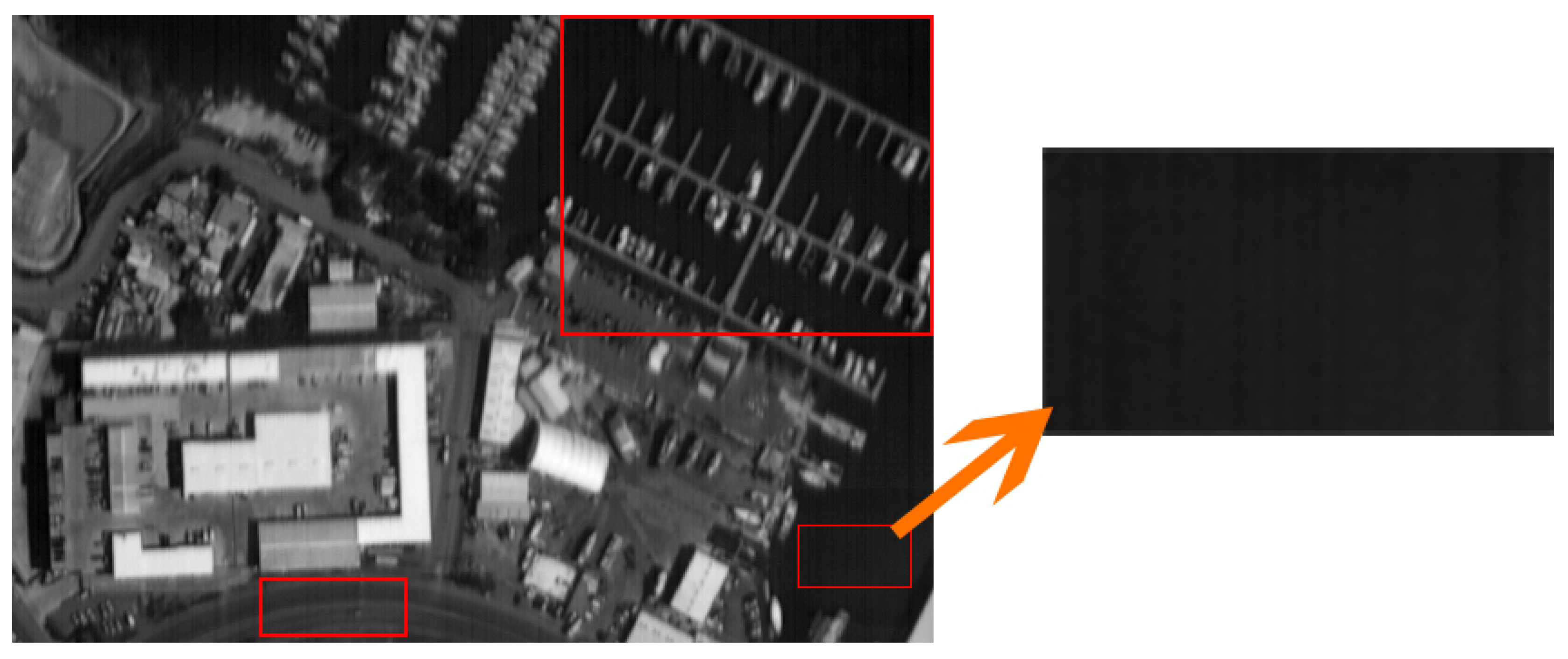
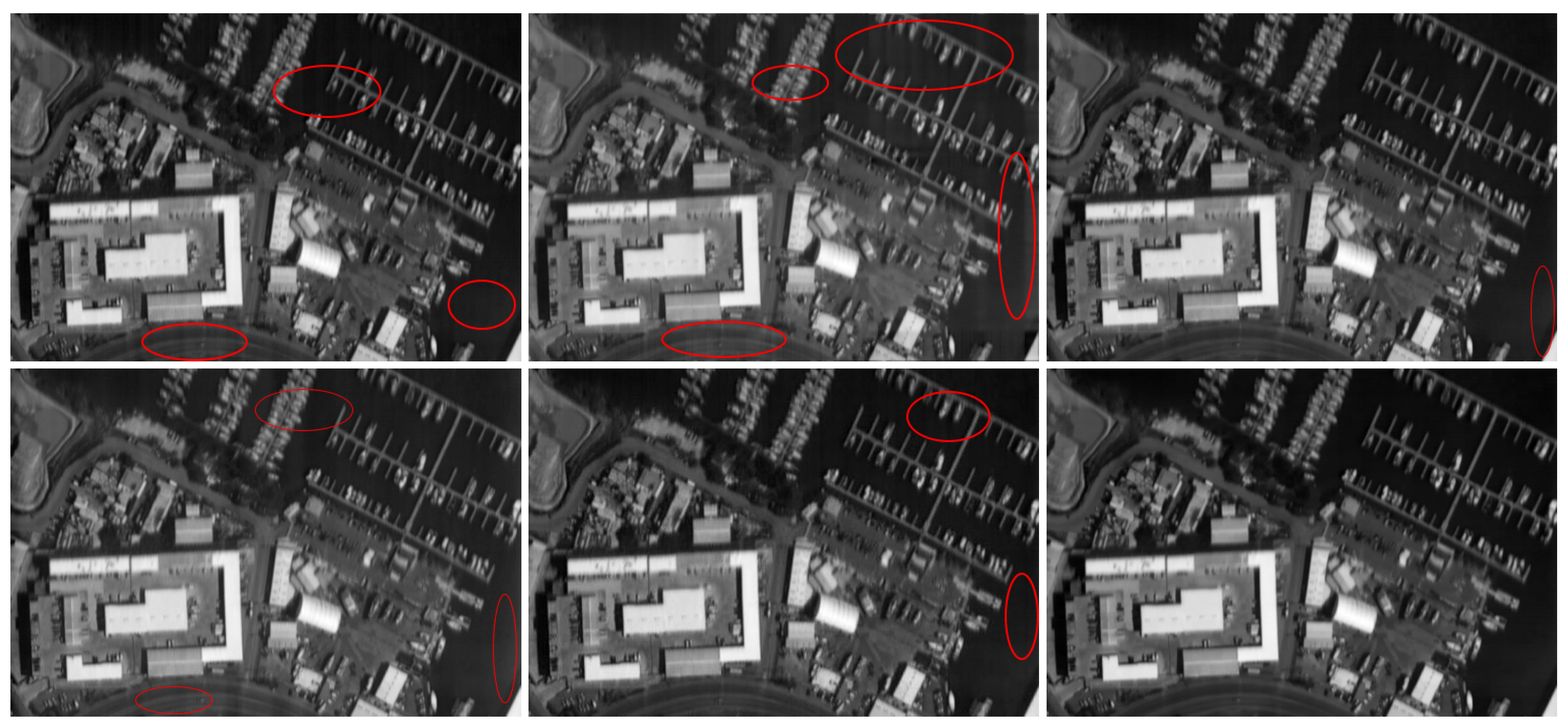
Figure 10 displays our data, with the uniform region utilized to calculate the PRNU, itself denoted by the rectangular box in the bottom-right corner. Table 5 depicts the PRNU. The proposed model is found to have the best performance, and the image’s PRNU decreases by 4.2%.
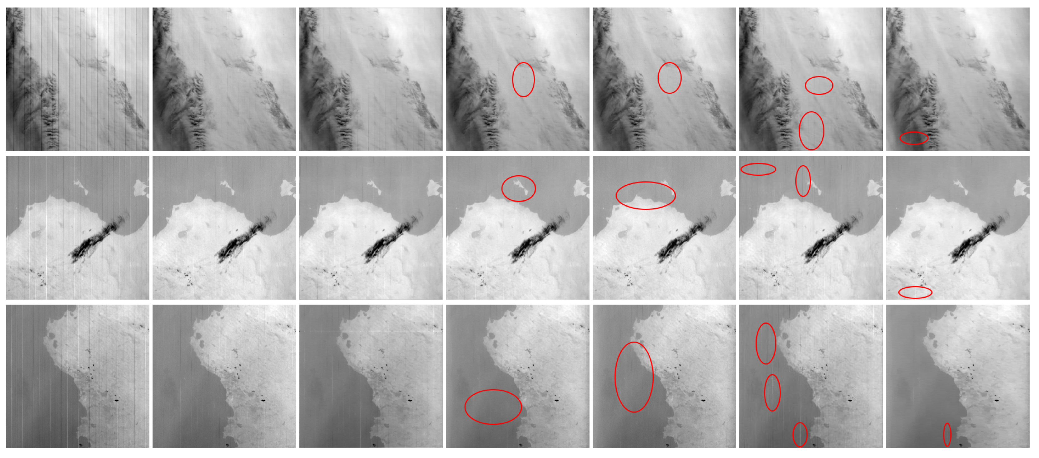
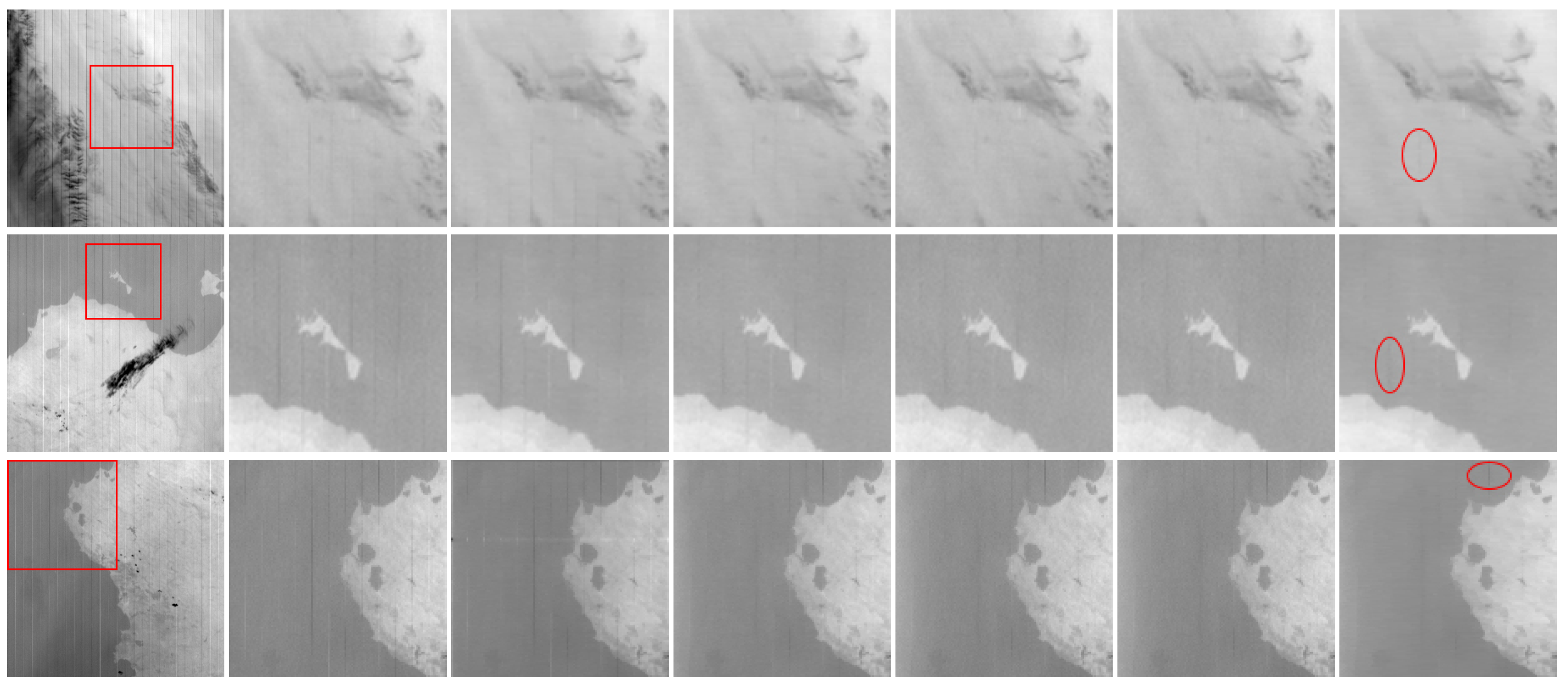
Additionally, we can get an intuitive comparison of MODIS data from Figure 11, and the red ellipses are used to mark the residual stripes in the images. Figure 12 is the enlarged processing effect of the rectangular region. Figure 13 shows the destriping results of our data, wherein ellipses are used to mark regions with a very poor removal effect. Figure 14 shows the partial enlargement of the rectangular region in the upper-right corner of Figure 10. The standard deviations of the images are shown in Table 6.
Considering the influence of excessive smoothing, it is necessary to integrate subjective and objective factors to evaluate models.
Table 6 demonstrates that the LRSID performs better on MODIS02. However, it is clear from the view of the destriping results in Figure 12 that SLD and LRSID do not completely remove stripes. Besides, the results in Figure 11 and Figure 12 show that the proposed model removes stripe noise more thoroughly, and the restored image is clearer, though there are still a few residual stripes in the regions marked by the red ellipse. From the results of processing our data, TVGS and the proposed model performed better; however, the proposed model obtained a clearer image with no ripple effects or residual stripes.
5. Discussion
5.1. Parameter Value Determination
The selection of appropriate parameters is very critical to the optimization model. There are five regularization parameters , , , , and two positive penalty parameters, and , in the proposed model. Empirical adjustment is the most commonly used method to determine the range of parameters. Over a large number of simulation experiments, the proposed model showed better robustness when the parameters change within a smaller range. We determined the range of parameter changes as follows: , , , . As for the , we selected for periodic stripes, and for non-periodic stripes.
5.2. Result Discussion
According to the results of all experiments, the proposed model can remove the stripe noise in most cases, but there are still some issues worth discussing. As can be seen from Table 1 and Table 3, the PSNR of the proposed model is always lower than that of other models when dealing with stripe noise of low intensity and ratio; in some cases, the gap is still large. It means that it cannot fully constrain the image prior and the stripe-noise prior in such case. The proposed model has several parameters that influence the destriping performance in various conditions, by determining the weight of each constraint item. When dealing with low-ratio and -intensity stripe noise, the low-rank feature can successfully constrain the stripe noise components; however, when dealing with high-noise-ratio and -intensity stripe noise, the sparsity feature constrains the stripe noise more effectively. We utilized the same parameters to achieve the destriping effect in different conditions during the experiments, to ensure the model’s reliability and practicability. This limited the weight of each constraint item, making it difficult to reach optimal constraints in some cases. Where stripes can be detected before removal, we can choose a more reasonable destriping model to achieve a better removal effect. Additionally, there is another problem in Figure 7. In the first and last few columns, the column mean values of the image restored by the proposed model are slightly different from those of the undegraded image. This could be have been caused by inappropriate border treatment, which could be improved in follow-up research.
5.3. Limitation
Although the proposed model achieves a superior destriping effect, it still has some limitations. The current research has mainly focused on removing stripe noise from a single remote sensing image, and the model is unable to perform destriping on remote sensing images with different channels, such as multispectral images. Furthermore, when there are some small fragment cases, the low-rank characteristics of the stripe components will be destroyed, significantly weakening the model’s stripe noise-removal effect. Therefore, when the image contains a lot of random noise, the model’s destriping effect may be considerably diminished.
6. Conclusions
The majority of image processing problems are ill-posed inverse problems that can be addressed with a suitable regularization model. The optimum result can be obtained by adding appropriate regularization terms to the underlying priors.
In this paper, under the premise of completely retaining the image information, we fully considered stripe noise’s potential low-rank and sparse properties and proposed a stable and effective destriping model. Constrained by these properties, the model can preserve image details while dealing with stripe noise. Combining the subjective and objective experimental results, the proposed model obtained better destriping performance than the other five existing typical models. Furthermore, the proposed model could still stably remove the stripe noise when other methods lost their effect. It shows an excellent stripe noise removal effect for different degrees of degraded images with strong robustness, and is, thus, worthy of promotion.
The proposed model shows strong competitiveness in both subjective and objective evaluation. However, it still has some problems, such as many solving processes, a large amount of calculation, and a long processing time, which will be continuously improved in follow-up research. In addition, random noise will pose a new challenge to the removal of stripe noise; whichever noise is preferentially processed will affect other types of noise. Therefore, related research will also be carried out in follow-up to remove all of types of noise simultaneously.
Author Contributions
Conceptualization, X.W., L.Z. and H.Q.; methodology, X.W. and L.Z.; writing—original draft preparation, X.W. and L.Z.; writing—review and editing, X.W., H.Q., L.Z., T.G. and Z.Z.; funding acquisition, L.Z. and H.Q. All authors have read and agreed to the published version of the manuscript.
Funding
This research was funded by the National Natural Science Foundation of China under Grant 62075219 and Grant 61805244; and the Key Technological Research Projects of Jilin Province, China under Grant 20190303094SF.
Institutional Review Board Statement
Not Applicable.
Informed Consent Statement
Not Applicable.
Data Availability Statement
The MODIS data used in this paper are available at the fllowing link: https://ladsweb.nascom.nasa.gov/, accessed on 15 November 2021. The hyperspectral image can be abtained from https://engineering.purdue.edu/~biehl/MultiSpec/, accessed on 15 November 2021. The source code of LRSID is available at http://www.escience.cn/people/changyi/index.html, accessed on 15 November 2021.
Acknowledgments
The authors would like to thank the anonymous reviewers for their valuable comments.
Conflicts of Interest
The authors declare no conflict of interest.
Abbreviations
The following abbreviations are used in this manuscript:
| TV | Total Variation |
| FIR | Finite Impulse Response |
| ADMM | Alternating Direction Multiplier Method |
| PSNR | Peak Signal to Noise Ratio |
| SSIM | Structural Similarity |
| PRNU | Photo Response Non-uniformity |
| SLD | Statistical Linear Destriping |
| LRSID | Low-Rank Single-Image Decomposition |
| GSLV | Global Sparsity and Local Variational |
| TVGS | Total Variation and Group Sparse |
References
- Pan, J.J.; Chang, C.I. Destriping of Landsat MSS images by filtering techniques. Photogramm. Eng. Remote Sens. 1992, 58, 1417. [Google Scholar]
- Simpson, J.J.; Gobat, J.I.; Frouin, R. Improved destriping of GOES images using finite impulse response filters. Remote Sens. Environ. 1995, 52, 15–35. [Google Scholar] [CrossRef]
- Torres, J.; Infante, S.O. Wavelet analysis for the elimination of striping noise in satellite images. Opt. Eng. 2001, 40, 1309–1314. [Google Scholar]
- Chen, J.; Shao, Y.; Guo, H.; Wang, W.; Zhu, B. Destriping CMODIS data by power filtering. IEEE Trans. Geosci. Remote Sens. 2003, 41, 2119–2124. [Google Scholar] [CrossRef]
- Chen, J.; Lin, H.; Shao, Y.; Yang, L. Oblique striping removal in remote sensing imagery based on wavelet transform. Int. J. Remote Sens. 2006, 27, 1717–1723. [Google Scholar] [CrossRef]
- Münch, B.; Trtik, P.; Marone, F.; Stampanoni, M. Stripe and ring artifact removal with combined wavelet—Fourier filtering. Opt. Express 2009, 17, 8567–8591. [Google Scholar] [CrossRef] [PubMed] [Green Version]
- Pal, M.K.; Porwal, A. Destriping of Hyperion images using low-pass-filter and local-brightness-normalization. In Proceedings of the 2015 IEEE International Geoscience and Remote Sensing Symposium (IGARSS), Milan, Italy, 26–31 July 2015; pp. 3509–3512. [Google Scholar]
- Pande-Chhetri, R.; Abd-Elrahman, A. De-striping hyperspectral imagery using wavelet transform and adaptive frequency domain filtering. ISPRS J. Photogramm. Remote Sens. 2011, 66, 620–636. [Google Scholar] [CrossRef]
- Horn, B.K.; Woodham, R.J. Destriping Landsat MSS images by histogram modification. Comput. Graph. Image Process. 1979, 10, 69–83. [Google Scholar] [CrossRef] [Green Version]
- Weinreb, M.; Xie, R.; Lienesch, J.; Crosby, D. Destriping GOES images by matching empirical distribution functions. Remote Sens. Environ. 1989, 29, 185–195. [Google Scholar] [CrossRef]
- Wegener, M. Destriping multiple sensor imagery by improved histogram matching. Int. J. Remote Sens. 1990, 11, 859–875. [Google Scholar] [CrossRef]
- Gadallah, F.; Csillag, F.; Smith, E. Destriping multisensor imagery with moment matching. Int. J. Remote Sens. 2000, 21, 2505–2511. [Google Scholar] [CrossRef]
- Sun, L.; Neville, R.; Staenz, K.; White, H.P. Automatic destriping of Hyperion imagery based on spectral moment matching. Can. J. Remote Sens. 2008, 34, S68–S81. [Google Scholar] [CrossRef]
- Rakwatin, P.; Takeuchi, W.; Yasuoka, Y. Restoration of Aqua MODIS Band 6 Using Histogram Matching and Local Least Squares Fitting. IEEE Trans. Geosci. Remote Sens. 2009, 47, 613–627. [Google Scholar] [CrossRef]
- Carfantan, H.; Idier, J. Statistical Linear Destriping of Satellite-Based Pushbroom-Type Images. IEEE Trans. Geosci. Remote Sens. 2010, 48, 1860–1871. [Google Scholar] [CrossRef]
- Shen, H.; Jiang, W.; Zhang, H.; Zhang, L. A piece-wise approach to removing the nonlinear and irregular stripes in MODIS data. Int. J. Remote Sens. 2014, 35, 44–53. [Google Scholar] [CrossRef]
- Shen, H.; Zhang, L. A MAP-Based Algorithm for Destriping and Inpainting of Remotely Sensed Images. IEEE Trans. Geosci. Remote Sens. 2009, 47, 1492–1502. [Google Scholar] [CrossRef]
- Bouali, M.; Ladjal, S. Toward Optimal Destriping of MODIS Data Using a Unidirectional Variational Model. IEEE Trans. Geosci. Remote Sens. 2011, 49, 2924–2935. [Google Scholar] [CrossRef]
- Lu, X.; Wang, Y.; Yuan, Y. Graph-Regularized Low-Rank Representation for Destriping of Hyperspectral Images. IEEE Trans. Geosci. Remote Sens. 2013, 51, 4009–4018. [Google Scholar] [CrossRef]
- Zhang, H.; Wei, H.; Zhang, L.; Shen, H.; Yuan, Q. Hyperspectral Image Restoration Using Low-Rank Matrix Recovery. IEEE Trans. Geosci. Remote Sens. 2014, 52, 4729–4743. [Google Scholar] [CrossRef]
- Chang, Y.; Fang, H.; Yan, L.; Liu, H. Robust destriping method with unidirectional total variation and framelet regularization. Opt. Express 2013, 21, 23307–23323. [Google Scholar] [CrossRef]
- Yi, C.; Yan, L.; Tao, W.; Sheng, Z. Remote Sensing Image Stripe Noise Removal: From Image Decomposition Perspective. IEEE Trans. Geosci. Remote Sens. 2016, 54, 7018–7031. [Google Scholar]
- Liu, X.; Lu, X.; Shen, H.; Yuan, Q.; Jiao, Y.; Zhang, L. Stripe Noise Separation and Removal in Remote Sensing Images by Consideration of the Global Sparsity and Local Variational Properties. IEEE Trans. Geosci. Remote Sens. 2016, 54, 3049–3060. [Google Scholar] [CrossRef]
- Chen, Y.; Huang, T.Z.; Zhao, X.L.; Deng, L.J.; Huang, J. Stripe noise removal of remote sensing images by total variation regularization and group sparsity constraint. Remote Sens. 2017, 9, 559. [Google Scholar] [CrossRef] [Green Version]
- Dou, H.X.; Huang, T.Z.; Deng, L.J.; Zhao, X.L.; Huang, J. Directional 0 Sparse Modeling for Image Stripe Noise Removal. Remote Sens. 2018, 10, 361. [Google Scholar] [CrossRef] [Green Version]
- Chang, Y.; Yan, L.; Fang, H.; Liu, H. Simultaneous Destriping and Denoising for Remote Sensing Images With Unidirectional Total Variation and Sparse Representation. IEEE Geosci. Remote Sens. Lett. 2014, 11, 1051–1055. [Google Scholar] [CrossRef]
- Yang, J.H.; Zhao, X.L.; Ma, T.H.; Chen, Y.; Huang, T.Z.; Ding, M. Remote sensing images destriping using unidirectional hybrid total variation and nonconvex low-rank regularization. J. Comput. Appl. Math. 2020, 363, 124–144. [Google Scholar] [CrossRef]
- Tikhonov, A.; Arsenin, V. Solutions of Ill-Posed Problems; Winston and Sons: Washington, DC, USA, 1977. [Google Scholar]
- Rudin, L.I.; Osher, S.; Fatemi, E. Nonlinear total variation based noise removal algorithms. Phys. D Nonlinear Phenom. 1992, 60, 259–268. [Google Scholar] [CrossRef]
- Qin, Z.; Goldfarb, D.; Ma, S. An Alternating Direction Method for Total Variation Denoising. Optim. Methods Softw. 2011, 30, 594–615. [Google Scholar] [CrossRef] [Green Version]
- Eckstein, J.; Bertsekas, D.P. On the Douglas-Rachford splitting method and the proximal point algorithm for maximal monotone operators. Math. Program. 1992, 55, 293–318. [Google Scholar] [CrossRef] [Green Version]
- Boyd, S.; Parikh, N.; Chu, E.; Peleato, B.; EcKstein, J. Distributed Optimization and Statistical Learning via the Alternating Direction Method of Multipliers. Found. Trends Mach. Learn. 2010, 3, 1–122. [Google Scholar] [CrossRef]
- Donoho, D.L. De-noising by soft-thresholding. IEEE Trans. Inf. Theory 2002, 41, 613–627. [Google Scholar] [CrossRef] [Green Version]
- Ng, M.K.; Chan, R.H.; Tang, W.C. A Fast Algorithm for Deblurring Models with Neumann Boundary Conditions. SIAM J. Sci. Comput. 1999, 21, 851–866. [Google Scholar] [CrossRef] [Green Version]
- Cai, J.F.; Candès, E.J.; Shen, Z. A Singular Value Thresholding Algorithm for Matrix Completion. SIAM J. Optim. 2010, 20, 1956–1982. [Google Scholar] [CrossRef]
- Blumensath, T.; Davies, M.E. Iterative Thresholding for Sparse Approximations. J. Fourier Anal. Appl. 2008, 14, 629–654. [Google Scholar] [CrossRef] [Green Version]
- Jiao, Y.; Jin, B.; Lu, X. A primal dual active set with continuation algorithm for the l(0)-regularized optimization problem. Appl. Comput. Harmon. Anal. 2015, 39, 400–426. [Google Scholar] [CrossRef]
- Zhou, W.; Bovik, A.C.; Sheikh, H.R.; Simoncelli, E.P. Image quality assessment: From error visibility to structural similarity. IEEE Trans. Image Process. 2004, 13, 600–612. [Google Scholar]
Figure 1.
Illustration of proposed model.

Figure 2.
Stripe image and its singular values.

Figure 3.
Destriping results of MODIS image under periodic stripes (From top to bottom, the noise attributes of ratio and intensity are respectively (0.3, 70), (0.5, 90), (0.7, 50), (0.9, 30). From left to right are the original image, degraded image, the destriping results of SLD, LRSID, TVGS, GSLV, HTVLR and the Proposed).

Figure 4.
Destriping results under non-periodic stripes (From top to bottom are hyperspectral image01 (0.5, 50), MODIS01 (0.3, 70), hyperspectral image02 (0.5, 90), MODIS02 (0.9, 30). From left to right are the original image, degraded image, the destriping results of SLD, LRSID, TVGS, GSLV, HTVLR and the Proposed).

Figure 5.
Stripe noise separated from the degraded image (From top to bottom are stripe noise of hyperspectral image01 (0.5, 50), MODIS01 (0.3, 70), hyperspectral image02 (0.5, 90), MODIS02 (0.9, 30). From left to right are the added stripe noise, the separation result of SLD, LRSID, TVGS, GSLV, HTVLR and the Proposed).

Figure 6.
Destriping results under high-intensity stripes (0.9, 80) (From left to right: the first row are the degraded image and the destriping results of SLD, LRSID, TVGS, GSLV, HTVLR and the Proposed; the second row are the added stripe noise and the stripe noise separated by SLD, LRSID, TVGS, GSLV, HTVLR and the Proposed).

Figure 7.
Comparison of the column mean value of the undegraded image and restored images in Figure 6 (From left to right: the first row are the results of the images restored by SLD and LRSID; the second row is the results of the images restored by TVGS and GSLV; the third row is the results of the images restored by HTVLR and the Proposed).

Figure 8.
Destriping results under different random noise forms (From top to bottom are the results of images containing Gaussian noise, Poisson noise, salt and pepper noise and speckle noise. From left to right are the degraded image, the destriping results of SLD, LRSID, TVGS, GSLV, HTVLR and the Proposed).

Figure 9.
Destriping results of non-remote sensing images (From top to bottom are the different images. From left to right are the original image, degraded image, the restored image and stripes separated by the proposed model).
Figure 9.
Destriping results of non-remote sensing images (From top to bottom are the different images. From left to right are the original image, degraded image, the restored image and stripes separated by the proposed model).

Figure 10.
Real remote sensing image and uniform region.

Figure 11.
Destriping results of MODIS remote sensing images (From top to bottom are MODIS01, MODIS02, MODIS03. From left to right are original image, the destriping results of SLD, LRSID, TVGS, GSLV, HTVLR and the Proposed).
Figure 11.
Destriping results of MODIS remote sensing images (From top to bottom are MODIS01, MODIS02, MODIS03. From left to right are original image, the destriping results of SLD, LRSID, TVGS, GSLV, HTVLR and the Proposed).

Figure 12.
Partially enlarged view of the destriping results of MODIS remote sensing images. (From top to bottom are MODIS01, MODIS02, MODIS03. From left to right are original image, the destriping results of SLD, LRSID, TVGS, GSLV, HTVLR and the Proposed).
Figure 12.
Partially enlarged view of the destriping results of MODIS remote sensing images. (From top to bottom are MODIS01, MODIS02, MODIS03. From left to right are original image, the destriping results of SLD, LRSID, TVGS, GSLV, HTVLR and the Proposed).

Figure 13.
Destriping result of the real remote sensing image (From left to right, the first row are the destriping results of SLD, LRSID and TVGS; the second row are the destriping results of GSLV, HTVLR and the Proposed).
Figure 13.
Destriping result of the real remote sensing image (From left to right, the first row are the destriping results of SLD, LRSID and TVGS; the second row are the destriping results of GSLV, HTVLR and the Proposed).

Figure 14.
Local processing results of real remote sensing images (From left to right, the first row are the destriping results of SLD, LRSID and TVGS; the second row are the destriping results of GSLV, HTVLR and the Proposed).
Figure 14.
Local processing results of real remote sensing images (From left to right, the first row are the destriping results of SLD, LRSID and TVGS; the second row are the destriping results of GSLV, HTVLR and the Proposed).


Table 1.
PSNR of different models under periodic stripe noise.
| Image | Method | r = 0.3 | r = 0.5 | r = 0.7 | r = 0.9 | ||||||||||||
|---|---|---|---|---|---|---|---|---|---|---|---|---|---|---|---|---|---|
| Intensity | Intensity | Intensity | Intensity | ||||||||||||||
| 30 | 50 | 70 | 90 | 30 | 50 | 70 | 90 | 30 | 50 | 70 | 90 | 30 | 50 | 70 | 90 | ||
| Hyperspectral image | SLD | 40.7623 | 40.3565 | 39.7621 | 33.1389 | 39.9614 | 38.6069 | 37.2848 | 35.9059 | 39.5197 | 37.6037 | 35.5704 | 14.6173 | 39.5197 | 37.6037 | 35.5040 | 14.6713 |
| LRSID | 35.3815 | 35.6900 | 35.7350 | 35.7470 | 35.8817 | 35.9247 | 35.9308 | 35.9474 | 35.8469 | 35.9239 | 35.9254 | 35.8749 | 35.8469 | 35.9239 | 35.9254 | 35.8749 | |
| TVGS | 39.0808 | 39.0958 | 39.0875 | 38.7651 | 38.4572 | 38.3999 | 38.4197 | 38.4480 | 37.8913 | 37.8211 | 37.7227 | 37.5384 | 37.8913 | 37.8211 | 37.7227 | 37.5384 | |
| GSLV | 35.7031 | 35.7143 | 35.7560 | 35.7098 | 35.6710 | 35.6377 | 35.6268 | 35.5980 | 35.6287 | 35.5391 | 35.4226 | 35.2289 | 35.6287 | 35.5391 | 35.4226 | 35.2289 | |
| HTVLR | 35.9175 | 32.8299 | 30.4946 | 28.6029 | 35.8070 | 32.8267 | 30.5155 | 28.6380 | 35.8323 | 32.8756 | 30.5558 | 28.6825 | 35.6965 | 32.7996 | 30.5307 | 28.6519 | |
| Proposed | 39.9943 | 39.2962 | 38.9919 | 38.8458 | 39.4150 | 38.6377 | 38.6793 | 38.9331 | 39.2052 | 38.6535 | 38.4616 | 38.1107 | 39.2052 | 38.6535 | 38.4616 | 38.1107 | |
| MODIS | SLD | 52.1371 | 51.4041 | 50.4967 | 49.5176 | 50.9999 | 48.9686 | 47.0117 | 45.2834 | 49.0407 | 47.5429 | 45.3456 | 43.4824 | 47.0761 | 44.8401 | 42.3219 | 40.3089 |
| LRSID | 39.9467 | 39.9152 | 39.9967 | 40.1257 | 40.1165 | 40.1547 | 40.1851 | 40.2119 | 40.1399 | 40.2250 | 40.3121 | 40.4414 | 39.7306 | 39.6969 | 39.6988 | 39.6793 | |
| TVGS | 47.9489 | 47.2767 | 47.0315 | 46.9728 | 48.9832 | 48.9284 | 48.7219 | 48.3933 | 47.5304 | 47.1522 | 47.2241 | 47.2893 | 44.2714 | 43.8235 | 42.9537 | 42.3731 | |
| GSLV | 40.3947 | 40.5206 | 40.7104 | 40.8861 | 41.0941 | 41.3768 | 41.6219 | 41.8463 | 40.9006 | 41.3199 | 41.8689 | 42.4452 | 40.2217 | 40.2402 | 40.4891 | 40.6818 | |
| HTVLR | 38.4765 | 34.1368 | 31.2640 | 29.0932 | 37.8805 | 33.9375 | 31.1168 | 28.9884 | 38.1052 | 33.9021 | 31.1079 | 28.9878 | 38.0341 | 33.8598 | 31.1145 | 28.9840 | |
| Proposed | 48.6227 | 46.9238 | 46.1389 | 45.9567 | 51.2011 | 50.9063 | 50.7519 | 50.6098 | 49.8948 | 49.4367 | 49.4704 | 49.7446 | 46.9948 | 44.9491 | 43.1214 | 42.8721 | |
Table 2.
SSIM of different models under periodic stripe noise.
| Image | Method | r = 0.3 | r = 0.5 | r = 0.7 | r = 0.9 | ||||||||||||
|---|---|---|---|---|---|---|---|---|---|---|---|---|---|---|---|---|---|
| Intensity | Intensity | Intensity | Intensity | ||||||||||||||
| 30 | 50 | 70 | 90 | 30 | 50 | 70 | 90 | 30 | 50 | 70 | 90 | 30 | 50 | 70 | 90 | ||
| Hyperspectral image | SLD | 0.9955 | 0.9946 | 0.9932 | 0.9911 | 0.9949 | 0.9926 | 0.9902 | 0.9841 | 0.9930 | 0.9876 | 0.9791 | 0.4314 | 0.9930 | 0.9876 | 0.9791 | 0.4314 |
| LRSID | 0.9918 | 0.9927 | 0.9930 | 0.9930 | 0.9939 | 0.9939 | 0.9939 | 0.9939 | 0.9934 | 0.9937 | 0.9937 | 0.9935 | 0.9934 | 0.9937 | 0.9937 | 0.9935 | |
| TVGS | 0.9964 | 0.9964 | 0.9963 | 0.9963 | 0.9960 | 0.9960 | 0.9960 | 0.9960 | 0.9953 | 0.9953 | 0.9953 | 0.9952 | 0.9953 | 0.9953 | 0.9953 | 0.9952 | |
| GSLV | 0.9910 | 0.9909 | 0.9908 | 0.9905 | 0.9910 | 0.9908 | 0.9899 | 0.9899 | 0.9908 | 0.9905 | 0.9900 | 0.9891 | 0.9908 | 0.9905 | 0.9900 | 0.9891 | |
| HTVLR | 0.9942 | 0.9917 | 0.9816 | 0.9836 | 0.9937 | 0.9911 | 0.9878 | 0.9832 | 0.9938 | 0.9914 | 0.9880 | 0.9836 | 0.9935 | 0.9912 | 0.9879 | 0.9831 | |
| Proposed | 0.9964 | 0.9964 | 0.9964 | 0.9963 | 0.9962 | 0.9962 | 0.9961 | 0.9961 | 0.9957 | 0.9956 | 0.9955 | 0.9955 | 0.9957 | 0.9956 | 0.9955 | 0.9953 | |
| MODIS | SLD | 0.9987 | 0.9982 | 0.9975 | 0.9966 | 0.9979 | 0.9959 | 0.9930 | 0.9892 | 0.9967 | 0.9926 | 0.9866 | 0.9785 | 0.9975 | 0.9949 | 0.9911 | 0.9860 |
| LRSID | 0.9983 | 0.9983 | 0.9983 | 0.9984 | 0.9983 | 0.9983 | 0.9983 | 0.9983 | 0.9983 | 0.9984 | 0.9984 | 0.9985 | 0.9983 | 0.9983 | 0.9983 | 0.9983 | |
| TVGS | 0.9991 | 0.9991 | 0.9991 | 0.9991 | 0.9991 | 0.9991 | 0.9991 | 0.9991 | 0.9990 | 0.9990 | 0.9990 | 0.9990 | 0.9989 | 0.9989 | 0.9988 | 0.9988 | |
| GSLV | 0.9982 | 0.9982 | 0.9981 | 0.9979 | 0.9982 | 0.9982 | 0.9981 | 0.9980 | 0.9982 | 0.9982 | 0.9981 | 0.9979 | 0.9981 | 0.9979 | 0.9976 | 0.9973 | |
| HTVLR | 0.9995 | 0.9989 | 0.9981 | 0.9944 | 0.9991 | 0.9982 | 0.9978 | 0.9967 | 0.9993 | 0.9987 | 0.9978 | 0.9967 | 0.9993 | 0.9986 | 0.9978 | 0.9967 | |
| Proposed | 0.9996 | 0.9996 | 0.9995 | 0.9995 | 0.9996 | 0.9996 | 0.9996 | 0.9996 | 0.9996 | 0.9996 | 0.9996 | 0.9996 | 0.9995 | 0.9994 | 0.9993 | 0.9992 | |
Table 3.
PSNR of different models under non-periodic stripe noise.
| Image | Method | r = 0.3 | r = 0.5 | r = 0.7 | r = 0.9 | ||||||||||||
|---|---|---|---|---|---|---|---|---|---|---|---|---|---|---|---|---|---|
| Intensity | Intensity | Intensity | Intensity | ||||||||||||||
| 30 | 50 | 70 | 90 | 30 | 50 | 70 | 90 | 30 | 50 | 70 | 90 | 30 | 50 | 70 | 90 | ||
| Hyperspectral image (01) | SLD | 35.3447 | 31.7048 | 29.0013 | 26.8673 | 32.0895 | 30.1640 | 27.4199 | 20.6502 | 32.2696 | 28.0868 | 23.0584 | 14.9193 | 30.6777 | 26.3734 | 19.3105 | 10.6051 |
| LRSID | 33.8233 | 31.4653 | 29.1579 | 27.0463 | 31.5824 | 30.3996 | 27.8443 | 25.5226 | 31.8777 | 28.2986 | 25.2156 | 22.5195 | 30.7139 | 26.5208 | 23.1218 | 20.3287 | |
| TVGS | 38.7072 | 36.2829 | 33.4100 | 30.6928 | 34.2652 | 33.9721 | 31.0179 | 28.3584 | 34.0143 | 30.0883 | 26.9076 | 24.2418 | 31.5150 | 27.7069 | 24.3439 | 21.4300 | |
| GSLV | 34.6330 | 32.8944 | 30.9638 | 29.0401 | 32.6877 | 31.6578 | 29.5419 | 27.5285 | 33.4977 | 30.3310 | 27.5669 | 25.0776 | 32.8353 | 29.7059 | 26.4824 | 23.4092 | |
| HTVLR | 35.0508 | 31.2176 | 28.9420 | 28.8632 | 33.5651 | 31.4572 | 27.5688 | 26.6761 | 33.0854 | 29.2073 | 25.5829 | 22.9086 | 31.8186 | 28.4824 | 24.1032 | 20.4523 | |
| Proposed | 35.1447 | 34.5641 | 33.9571 | 33.2269 | 33.4716 | 33.6839 | 32.7429 | 31.7382 | 34.8838 | 33.6992 | 32.2696 | 30.8142 | 34.2725 | 33.5532 | 32.6933 | 31.6803 | |
| MODIS(01) | SLD | 37.3381 | 33.2820 | 30.4637 | 28.3107 | 34.3412 | 29.9283 | 26.9709 | 24.7386 | 32.2575 | 27.8777 | 24.9191 | 18.5936 | 31.9292 | 27.5246 | 24.5699 | 12.1103 |
| LRSID | 35.0517 | 32.4045 | 29.9019 | 27.7256 | 32.8137 | 29.0122 | 26.0444 | 23.6232 | 31.3061 | 26.9440 | 23.6602 | 21.0059 | 31.1085 | 26.9318 | 23.6982 | 20.9615 | |
| TVGS | 42.0600 | 38.6558 | 35.1310 | 32.1397 | 36.6404 | 31.9843 | 28.4645 | 25.7084 | 33.4679 | 28.9072 | 25.4481 | 22.6511 | 31.3206 | 27.4750 | 24.5042 | 22.0021 | |
| GSLV | 37.3673 | 34.8319 | 32.4582 | 30.3732 | 35.0774 | 31.5064 | 28.5077 | 25.9658 | 33.1705 | 30.1618 | 26.8225 | 23.9861 | 31.9486 | 28.9601 | 25.8517 | 23.2652 | |
| HTVLR | 34.7274 | 32.9110 | 29.5728 | 26.8078 | 32.2557 | 30.2083 | 28.2044 | 25.2784 | 33.0159 | 28.2989 | 25.7874 | 22.3446 | 31.8347 | 27.0853 | 23.9765 | 22.4003 | |
| Proposed | 34.3651 | 33.9262 | 33.3634 | 32.6629 | 33.2117 | 32.1403 | 31.0206 | 29.8827 | 33.7232 | 33.1588 | 32.4502 | 31.5701 | 32.3019 | 30.6507 | 29.0172 | 27.4448 | |
| Hyperspectral image (02) | SLD | 36.2916 | 31.9875 | 29.0546 | 26.8216 | 35.3499 | 31.0813 | 28.1446 | 20.0484 | 32.9993 | 28.6127 | 22.3813 | 13.4758 | 31.0791 | 26.6511 | 17.7244 | 10.3148 |
| LRSID | 35.7304 | 32.4357 | 29.7151 | 27.4146 | 35.5710 | 31.9302 | 28.9187 | 26.3609 | 33.3114 | 29.3193 | 26.1621 | 23.4309 | 31.7662 | 27.0848 | 23.5241 | 20.6438 | |
| TVGS | 43.9596 | 39.5005 | 35.1955 | 31.7593 | 42.8190 | 37.4688 | 33.1838 | 29.9043 | 35.2863 | 30.9347 | 27.7148 | 25.0720 | 32.8635 | 28.3649 | 24.7524 | 21.7456 | |
| GSLV | 38.9853 | 35.2414 | 32.2460 | 29.7611 | 38.1829 | 34.5052 | 31.5713 | 29.1273 | 35.9022 | 31.8174 | 28.6891 | 26.0784 | 36.1973 | 31.3977 | 27.3928 | 23.9869 | |
| HTVLR | 36.4678 | 33.5402 | 31.8486 | 28.3441 | 36.2421 | 32.8050 | 29.4345 | 25.6534 | 34.8462 | 29.8140 | 25.6910 | 22.6884 | 33.6814 | 28.8084 | 24.0925 | 22.1252 | |
| Proposed | 39.2506 | 37.5226 | 35.8696 | 34.3269 | 39.3499 | 38.1468 | 36.7722 | 35.3357 | 37.3850 | 35.3551 | 33.4955 | 31.8256 | 38.0805 | 36.6378 | 35.1649 | 33.6987 | |
| MODIS(02) | SLD | 37.5798 | 33.4708 | 30.6264 | 28.4564 | 33.8344 | 29.6296 | 26.7684 | 24.5903 | 32.3259 | 27.9541 | 24.1494 | 18.4432 | 32.0122 | 27.6443 | 24.2635 | 11.8774 |
| LRSID | 34.8305 | 32.1984 | 29.7625 | 27.6320 | 32.7221 | 28.9821 | 26.0387 | 23.6293 | 31.3837 | 27.0681 | 23.7680 | 21.0766 | 31.7608 | 27.4014 | 24.0023 | 21.1461 | |
| TVGS | 40.0048 | 37.1845 | 34.1550 | 31.5341 | 35.7214 | 31.5371 | 28.2808 | 25.6356 | 33.4506 | 29.0122 | 25.6242 | 22.8340 | 32.3990 | 28.2698 | 25.0687 | 22.3843 | |
| GSLV | 35.0578 | 33.2712 | 31.4417 | 29.7087 | 33.7419 | 30.8448 | 28.1933 | 25.8462 | 33.6929 | 29.2312 | 26.9986 | 24.1839 | 33.3650 | 29.6181 | 26.4697 | 23.7723 | |
| HTVLR | 36.1366 | 31.1110 | 29.7969 | 27.3224 | 34.9065 | 30.9915 | 26.9208 | 24.6307 | 33.3510 | 30.5450 | 24.1067 | 22.8506 | 32.4660 | 26.7465 | 25.0747 | 23.1931 | |
| Proposed | 31.2816 | 30.5062 | 29.8869 | 29.3222 | 31.6262 | 30.9520 | 30.2050 | 29.3541 | 30.8442 | 29.9709 | 29.1658 | 28.3991 | 31.1998 | 30.1065 | 28.8306 | 27.5111 | |
Table 4.
SSIM of different models under non-periodic stripe noise.
| Image | Method | r = 0.3 | r = 0.5 | r = 0.7 | r = 0.9 | ||||||||||||
|---|---|---|---|---|---|---|---|---|---|---|---|---|---|---|---|---|---|
| Intensity | Intensity | Intensity | Intensity | ||||||||||||||
| 30 | 50 | 70 | 90 | 30 | 50 | 70 | 90 | 30 | 50 | 70 | 90 | 30 | 50 | 70 | 90 | ||
| Hyperspectral image (01) | SLD | 0.9921 | 0.9844 | 0.9728 | 0.9570 | 0.9879 | 0.9770 | 0.9601 | 0.8346 | 0.9875 | 0.9707 | 0.9066 | 0.5559 | 0.9810 | 0.9546 | 0.8046 | 0.1775 |
| LRSID | 0.9917 | 0.9882 | 0.9813 | 0.9698 | 0.9889 | 0.9850 | 0.9747 | 0.9568 | 0.9889 | 0.9785 | 0.9563 | 0.9119 | 0.9853 | 0.9647 | 0.9254 | 0.8630 | |
| TVGS | 0.9959 | 0.9945 | 0.9917 | 0.9864 | 0.9934 | 0.9922 | 0.9879 | 0.9805 | 0.9923 | 0.9863 | 0.9745 | 0.9534 | 0.9881 | 0.9755 | 0.9487 | 0.9021 | |
| GSLV | 0.9903 | 0.9884 | 0.9852 | 0.9797 | 0.9890 | 0.9868 | 0.9827 | 0.9763 | 0.9890 | 0.9839 | 0.9751 | 0.9603 | 0.9886 | 0.9825 | 0.9677 | 0.9362 | |
| HTVLR | 0.9922 | 0.9876 | 0.9788 | 0.9772 | 0.9902 | 0.9861 | 0.9657 | 0.9649 | 0.9913 | 0.9791 | 0.9623 | 0.9294 | 0.9874 | 0.9748 | 0.9341 | 0.8770 | |
| Proposed | 0.9907 | 0.9902 | 0.9897 | 0.9890 | 0.9900 | 0.9895 | 0.9886 | 0.9874 | 0.9905 | 0.9895 | 0.9881 | 0.9860 | 0.9901 | 0.9895 | 0.9886 | 0.9875 | |
| MODIS(01) | SLD | 0.9912 | 0.9796 | 0.9634 | 0.9436 | 0.9850 | 0.9625 | 0.9322 | 0.8968 | 0.9757 | 0.9403 | 0.8955 | 0.7501 | 0.9782 | 0.9463 | 0.9043 | 0.3482 |
| LRSID | 0.9931 | 0.9851 | 0.9708 | 0.9486 | 0.9875 | 0.9643 | 0.9273 | 0.8767 | 0.9796 | 0.9382 | 0.8757 | 0.7974 | 0.9846 | 0.9509 | 0.8828 | 0.7828 | |
| TVGS | 0.9979 | 0.9958 | 0.9917 | 0.9848 | 0.9946 | 0.9856 | 0.9663 | 0.9355 | 0.9896 | 0.9685 | 0.9276 | 0.8693 | 0.9889 | 0.9712 | 0.9361 | 0.8759 | |
| GSLV | 0.9949 | 0.9925 | 0.9888 | 0.9833 | 0.9935 | 0.9870 | 0.9740 | 0.9510 | 0.9908 | 0.9792 | 0.9564 | 0.9154 | 0.9586 | 0.9821 | 0.9631 | 0.9270 | |
| HTVLR | 0.9907 | 0.9856 | 0.9694 | 0.9452 | 0.9848 | 0.9724 | 0.9508 | 0.9101 | 0.9878 | 0.9597 | 0.9254 | 0.8656 | 0.9810 | 0.9529 | 0.9065 | 0.8160 | |
| Proposed | 0.9947 | 0.9942 | 0.9936 | 0.9930 | 0.9945 | 0.9937 | 0.9926 | 0.9911 | 0.9945 | 0.9939 | 0.9931 | 0.9920 | 0.9940 | 0.9925 | 0.9902 | 0.9869 | |
| Hyperspectral image (02) | SLD | 0.9757 | 0.9401 | 0.8936 | 0.8427 | 0.9710 | 0.9330 | 0.8814 | 0.6978 | 0.9462 | 0.8703 | 0.7073 | 0.2751 | 0.9270 | 0.8403 | 0.5567 | 0.0625 |
| LRSID | 0.9804 | 0.9533 | 0.9131 | 0.8648 | 0.9818 | 0.9586 | 0.9205 | 0.8648 | 0.9596 | 0.8989 | 0.8184 | 0.7155 | 0.9455 | 0.8670 | 0.7638 | 0.6477 | |
| TVGS | 0.9949 | 0.9871 | 0.9676 | 0.9347 | 0.9943 | 0.9858 | 0.9696 | 0.9422 | 0.9710 | 0.9302 | 0.8702 | 0.7975 | 0.9536 | 0.8967 | 0.8125 | 0.7134 | |
| GSLV | 0.9874 | 0.9737 | 0.9489 | 0.9114 | 0.9855 | 0.9720 | 0.9518 | 0.9238 | 0.9736 | 0.9397 | 0.8906 | 0.8287 | 0.9756 | 0.9396 | 0.8783 | 0.7906 | |
| HTVLR | 0.9756 | 0.9632 | 0.9421 | 0.8749 | 0.9794 | 0.9477 | 0.9042 | 0.8063 | 0.9709 | 0.8986 | 0.8041 | 0.7174 | 0.9642 | 0.9113 | 0.7597 | 0.6956 | |
| Proposed | 0.9864 | 0.9828 | 0.9778 | 0.9713 | 0.9865 | 0.9835 | 0.9790 | 0.9726 | 0.9793 | 0.9697 | 0.9564 | 0.9395 | 0.9830 | 0.9771 | 0.9686 | 0.9572 | |
| MODIS(02) | SLD | 0.9732 | 0.9481 | 0.9223 | 0.8957 | 0.9568 | 0.9204 | 0.8800 | 0.8367 | 0.9489 | 0.9056 | 0.8354 | 0.6898 | 0.9508 | 0.9083 | 0.8485 | 0.3042 |
| LRSID | 0.9795 | 0.9535 | 0.9250 | 0.8941 | 0.9641 | 0.9239 | 0.8741 | 0.8132 | 0.9549 | 0.9047 | 0.8325 | 0.7407 | 0.9570 | 0.9068 | 0.8312 | 0.7263 | |
| TVGS | 0.9973 | 0.9921 | 0.9826 | 0.9639 | 0.9849 | 0.9686 | 0.9325 | 0.8879 | 0.9694 | 0.9408 | 0.8979 | 0.8341 | 0.9669 | 0.9354 | 0.8868 | 0.8148 | |
| GSLV | 0.9855 | 0.9768 | 0.9644 | 0.9466 | 0.9781 | 0.9633 | 0.9390 | 0.8997 | 0.9674 | 0.9461 | 0.9185 | 0.8754 | 0.9700 | 0.9501 | 0.9206 | 0.8705 | |
| HTVLR | 0.9779 | 0.9326 | 0.9177 | 0.8988 | 0.9740 | 0.9385 | 0.9068 | 0.8515 | 0.9607 | 0.9252 | 0.8607 | 0.8199 | 0.9552 | 0.9055 | 0.8469 | 0.7995 | |
| Proposed | 0.9740 | 0.9733 | 0.9721 | 0.9697 | 0.9750 | 0.9694 | 0.9597 | 0.9485 | 0.9645 | 0.9589 | 0.9538 | 0.9488 | 0.9625 | 0.9549 | 0.9461 | 0.9357 | |
Table 5.
PRNU of uniform region.
| Method | Original | SLD | LRSID | TVGS | GSLV | HTVLR | Proposed |
|---|---|---|---|---|---|---|---|
| PRNU | 0.1039 | 0.0939 | 0.0675 | 0.0762 | 0.0795 | 0.1009 | 0.0619 |
Table 6.
Standard deviations of images (sigma).
| Original | SLD | LRSID | TVGS | GSLV | HTVLR | Proposed | |
|---|---|---|---|---|---|---|---|
| MODIS01 | 49.6308 | 48.7199 | 46.7413 | 47.4065 | 45.5546 | 48.2170 | 39.8696 |
| MODIS02 | 30.3869 | 30.1396 | 29.7943 | 30.0316 | 30.0455 | 30.1504 | 29.9884 |
| MODIS03 | 32.4919 | 32.2129 | 30.7052 | 31.2176 | 30.0831 | 32.0267 | 30.0383 |
| Our data | 42.6685 | 42.4436 | 41.9675 | 42.3616 | 42.1085 | 42.5861 | 41.3120 |
Publisher’s Note: MDPI stays neutral with regard to jurisdictional claims in published maps and institutional affiliations. |
© 2021 by the authors. Licensee MDPI, Basel, Switzerland. This article is an open access article distributed under the terms and conditions of the Creative Commons Attribution (CC BY) license (https://creativecommons.org/licenses/by/4.0/).
Share and Cite
MDPI and ACS Style
Wu, X.; Qu, H.; Zheng, L.; Gao, T.; Zhang, Z. A Remote Sensing Image Destriping Model Based on Low-Rank and Directional Sparse Constraint. Remote Sens. 2021, 13, 5126. https://0-doi-org.brum.beds.ac.uk/10.3390/rs13245126
AMA Style
Wu X, Qu H, Zheng L, Gao T, Zhang Z. A Remote Sensing Image Destriping Model Based on Low-Rank and Directional Sparse Constraint. Remote Sensing. 2021; 13(24):5126. https://0-doi-org.brum.beds.ac.uk/10.3390/rs13245126
Chicago/Turabian StyleWu, Xiaobin, Hongsong Qu, Liangliang Zheng, Tan Gao, and Ziyu Zhang. 2021. "A Remote Sensing Image Destriping Model Based on Low-Rank and Directional Sparse Constraint" Remote Sensing 13, no. 24: 5126. https://0-doi-org.brum.beds.ac.uk/10.3390/rs13245126
Note that from the first issue of 2016, this journal uses article numbers instead of page numbers. See further details here.