1. Introduction
Soil moisture is a key state variable with multiple inter relationships with the functioning of terrestrial ecosystems [
1]. Besides, it is one of the Global Climate Observing System (GCOS), Essential Climate Variables (ECV), as well as one of the European Space Agency (ESA) Climate Change Initiative (CCI) variables. The role of soil water content at or near the soil surface is a well-recognized fact [
2]. A large variety of Earth system interactions take place in this thin topsoil layer because the water and energy fluxes between the continental surface and the atmosphere strongly depend on soil moisture in this layer [
3]. Soil moisture content is associated to a large collection of factors, so predicting its temporal and spatial variations may provide useful information in fields such as ecology, biogeochemical cycles, climate monitoring and water management among others [
4,
5,
6,
7].
SMOS is the second Earth Explorer Opportunity mission (launched in November 2009) developed as part ESA Living Planet Programme, and it was designed to obtain surface soil moisture and sea surface salinity data with global coverage and temporary regularity, using a low microwave frequency—L-band (1.4 GHz)—[
8,
9,
10]. As a contribution to the SMOS mission, [
11] developed a Project on the “Validation of SMOS Products over Mediterranean Ecosystem Vegetation at the Valencia Anchor Station Reference Area” (SMOS Cal/Val AO I.D. no. 3252). In this context, the Valencia Anchor Station (VAS) experimental site, in eastern Spain, was chosen as a primary validation site for SMOS [
12,
13]. The realization of field validation activities for any Earth Observation mission always has a significant component of preparation and preliminary developments that is often a complex task, and accurate and reliable soil moisture estimates have important implications in this case. Since 2001, and in order to understand the spatiotemporal organization of soil moisture in semiarid Mediterranean ecosystems, the University of Valencia has been carrying out the necessary activities to develop a network of stations to obtain soil moisture measurements in the VAS area that can be used to validate SMOS land products. Such activities have produced a significant characterization of the area at the scale of the SMOS pixel (50 × 50 km
2), more thoroughly in a control area of (10 × 10 km
2), all this facilitating its selection as a core validation site [
14].
The variation in the water content at a given point in the soil will depend partially on the degree of variability of the local edaphic properties, and its importance will be conditioned by the scale of the spatiotemporal analysis. From a general viewpoint, it is possible to distinguish between local detailed scale and regional scale [
2]. At detailed scale a set of local factors such as topography, hydrodynamic soil properties (texture, organic matter, structure and macroporosity) and vegetation cover will be able to explain the differences [
15,
16,
17] whereas at regional scale the climatic factors will be crucial [
18]. The area comprising the SMOS pixel may be considered sufficiently homogeneous from the climatic viewpoint. However, when the study requires a more detailed scale, new sampling strategies need to be established in order to be able to account for the landscape fragmentation, typical of the Mediterranean crop and vegetation mosaic distribution, the varying physiography, and the different geological materials that influence the more local factors of which soil moisture depends. The different sampling strategies carried out at the VAS in the framework of the SMOS validation campaigns of 2008, 2009 and 2010 is a good example of this and the respective sampling strategies were thus defined at different scales depending on the specific area under study.
The landscape subdivision into physio-hydrological units (SMOS units) has revealed itself to be a satisfactory tool to establish a stratified sampling of unit classes presenting a certain degree of internal uniformity with respect to hydrological parameters [
19,
20,
21,
22] and to capture the spatial and temporal variation of soil moisture at the local fine scale. Most land surface models (LSMs) require knowledge of soil hydrological parameters. These parameters are often derived from soil texture information, but due to the heterogeneous nature of soils and lack of detailed maps of soil properties, soil parameterization schemes are often simple, inflexible or inappropriate [
23]. The knowledge and quantification of soil hydrological parameters such as texture, organic matter, structure and bulk density, as well as the anthropic factors capable of modifying them, allow for more flexibility to reproduce real averaged conditions [
24].
In this paper we present the results of an extensive analysis of the hydrodynamic properties of the soil in the area of influence of the VAS using spatial and temporal effects by implementing statistical modeling with emphasis to understand the factors that control the variability of soil moisture in the study area. We consider a Bayesian statistical context to fit spatio-temporal statistical models related to the local expected soil moisture. We use Stochastic Partial Differential Equation (SPDE) with Integrated Nested Laplace Approximation (INLA) [
25,
26]. These methodologies have been highly developed and applied, e.g., [
27,
28,
29] and constitute one step ahead of the classical Geostatistics with kriging.
The rest of the paper is organized as follows.
Section 2 gives details on the materials used and on the complete methodology,
Section 3 is devoted to the results of the study,
Section 4 gives the discussion on the statistical modelling and
Section 5 provides the Conclusions.
2. Materials and Methods
2.1. Site Description
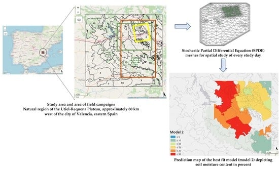
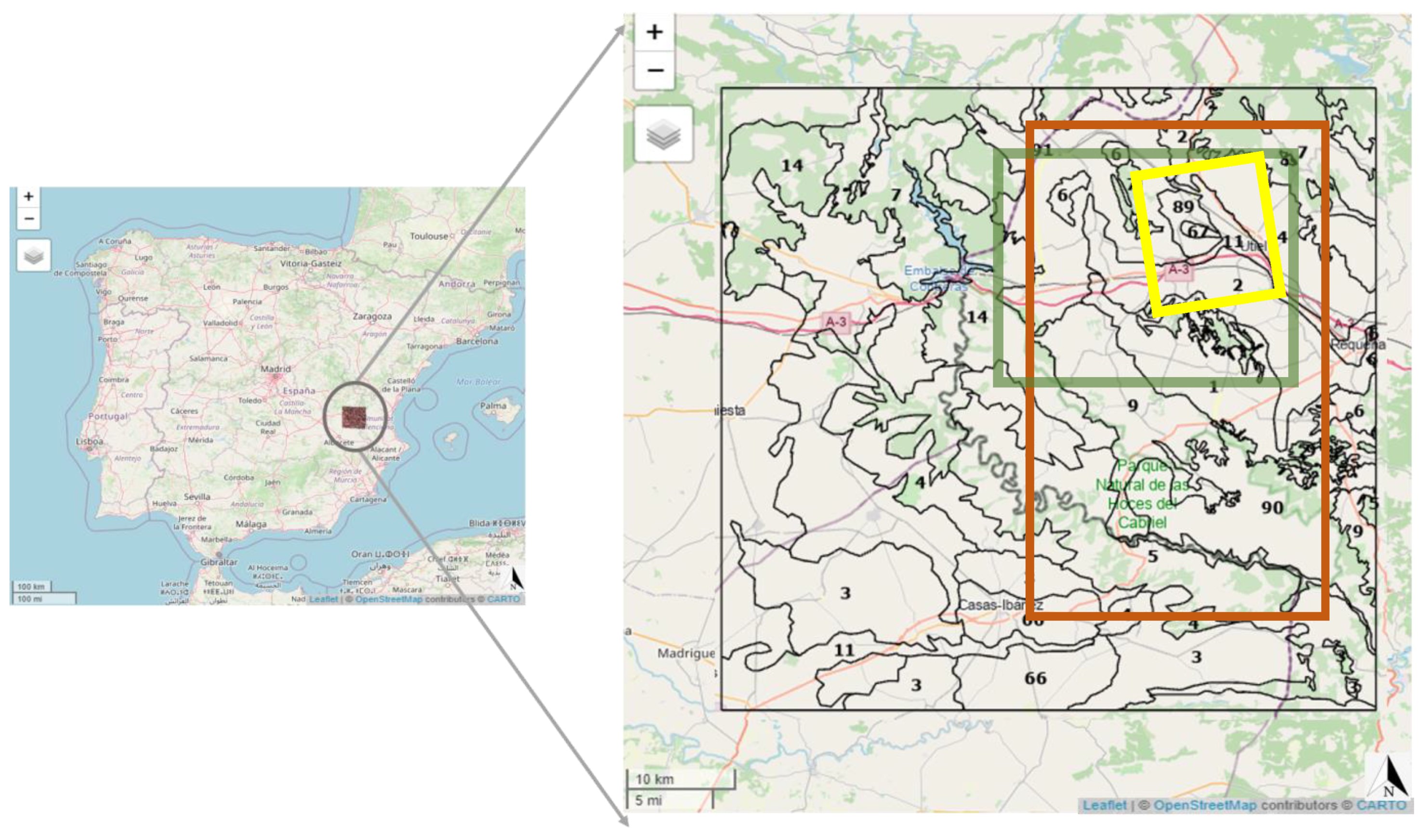
The site selected (
Figure 1), as a core validation for SMOS land products, is a typical Mediterranean sparse vegetation ecosystem defined within the natural region of the Utiel-Requena Plateau, at about 80 km W of the city of Valencia, eastern Spain. The actual meteorological station that gives the name to the site was been installed (N 39.570740°, W −1.288176°) in November 2001, and represents a reasonably homogeneous area of about 50 × 50 km
2 with an extend of NW: 1.698423W, 39.683639N; NE: 1.115635W, 39.675642N; SE: 1.127737W, 39.225365N; SW: 1.706786W, 39.233235N (UTM ED50). The main land use is vineyards with the presence of other typical Mediterranean ecosystem components such as olive and almond trees and shrubs, oaks, pine and cereal.
The area remains mostly under bare soil conditions outside the vineyard growing season. The climate is semi-arid (D d B’2 b’3), mesothermic, without excess water in winter and more than 53% potential evapotranspiration. The climate in the area has also been classified as dry–sub-humid (C1 d B’1 b’4) [
30]. Topography is mostly flat in a control area of about 10 × 10 km
2 with an extent of NW: 643966, 4386507; NE: 653735, 4388886; SE: 655995, 4378531; SW: 646226, 4376152 (UTM ED50) defined within the 50 × 50 km
2 one, surrounded by more abrupt and topographically complex zones. According to the FAO soil classification (FAO, 2006) soil types correspond to Haplic and Petric Calcisols or Calcaric Cambisols, and Fluvisols in the Magro River area, appearing as Regosols, Leptosols and punctually Kastanozems, in the natural vegetation zones of the mountain ranges that make up the area.
2.2. Experimental Design and Soil Sampling
Soil data used in this study were collected in 2008 (SMOS Validation Rehearsal Campaign) [
31,
32,
33] (CNES CAROLS Campaign 2009) and 2010 (ESA-CNES CAROLS Campaign 2010) [
34,
35]. These field and airborne campaigns took place on 22, 24, 28 April and 2 May 2008, over the VAS control area (10 × 10 km
2); 27 April, 19 and 28 May 2009, over an area of 25 × 48 km
2 inside the SMOS reference pixel and including the previous control area; and 5, 28 May and 10, 23 June 2010, in an area of 20.5 × 26.5 km
2 in the center of the SMOS reference pixel [
22]. The campaigns included extensive airborne passive microwave observations together with spatially distributed in situ ground measurements [
34,
36,
37].
In the plots selected in each campaign, during the on-site collection usually 3 to 4 replicated metal cylinders of volume 90.4 cm
3 (5.0 cm in height and a diameter of 4.8 cm) were obtained at each sampling plot. These soil cylinders, adequately manipulated, allowed to work in conditions of non-alteration from a structural viewpoint. The total number of samplings for all the campaigns implied the acquisition of more than 15,500 metal cylinders. Previously to the campaigns, a combined soil sampling was taken in more than 350 of the selected plots to characterize soil texture and/or organic matter content. A more detailed description of strategies for obtaining the data can be found in [
20,
21,
32,
33].
2.3. Analysis of Soil Properties
The analyses were carried out following [
38,
39]. The parameters thus determined were gravimetric water content (mass of water per mass of soil) and volumetric water content θ m
3/m
3 (volume of water per total volume of soil); soil bulk density, (δ
bulk), by weighting the undisturbed sample taken in the metal cylinder of known volume once dried in a stove for 24 h at 105 °C; porosity (ŋ) from its inverse relationship to bulk and particle density, δ
real, (2.65 g/cm
3; weighted average of soil solid particles densities) ŋ = 1 − (δ
bulk/δ
real); particle-size distribution determined by the hydrometer methodology; and soil organic matter content determined by oxidation with potassium dichromate.
2.4. Statistical Analysis
The aim of the statistical analysis in this work is to assess the effect that covariate related to soil properties have on soil moisture contents and to identify those covariates that show a statistically significant association with soil moisture content. To tackle this task, the Integrated Nested Laplace Approximation (INLA) [
25,
26] approach was applied to identify the variables that affect moisture. The advantage of using INLA over other methods, such as basic statistical methods, or other more complex methods, such as Markov Change Monte Carlo (MCMC) or Generalized Linear Models (GLM), is that INLA works in reasonable computational times by allowing the user to quickly and efficiently work with complex models [
25,
28,
29] allows as many covariates as desired to be integrated, and even incorporate new ones into the model in later steps and it does not require any work being conducted exclusively with normal distributions as it is based on Bayesian inference.
2.4.1. Integrated Nested Laplace Approximation (INLA)
This work offers then the possibility of analyzing the data by using INLA. The data can be idealized as realizations of a stochastic process indexed by:
where the study area
D is a subset of
.
The data can be presented by a collection of observations
[
25]. In statistical analysis, to estimate a general model, it is useful to model the mean for the unit using an additive linear predictor, defined on a suitable scale:
where
is the linear predictor which relates the expected value of the response variable with a linear combination of the covariates and the spatial term through the link function
;
are the coefficients that quantify the effect of covariates
zj = (
z1j,…,
zMj) on the response, and
f = {
f1(.),…,
fL(.)} is a collection of functions defined in terms of a set of covariates ν = (
ν1,…,
νL) that include the random effects as well as the spatially correlated effect. This spatial effect is a random effect itself because we don’t know its structure completely, and it is introduced as a random field with Matérn covariance structure.
This statistical analysis can be carried out with the open-source statistical package R, version 3.6.0 [
40] and the R-INLA package 2020 [
41]. All computations were conducted on a quad-core Intel i7-4790 (3.60 GHz) processor with 16 GB (DDR3-1333/1600) RAM. Different models can be obtained depending on the covariates considered for each one. Once the collection of competing models has been obtained, the DIC (Deviance Information Criterion) can be obtained for each one of them in order to select the best one. The best models would be those with a high level of complexity and a high goodness-of-fit, and models to be chosen should be those that show the lowest DIC [
29]:
where
is the deviance evaluated at the posterior mean of the model parameters and
denotes the ‘effective number of parameters’, which measures the complexity of the model [
29]. When the model is correct,
should approximately equal the ‘effective degrees of freedom’,
.
For each model, a covariate Xi is significant in relation to the response variable Yi if there is no change in the sign between the 0.025 quantile and the 0.975 quantile of the mean of the corresponding . In addition, the positive sign of the mean of the corresponding implies that the response variable increases when the covariate increases. The higher the mean of is, the more significant the covariate will be.
2.4.2. Stochastic Partial Differential Equation (SPDE)
R software [
40] and the Bayesian estimation methodology, including the basic features of INLA approach and the SPDE [
25,
26], were used to fit parametric models to the observed spatial patterns, including covariates that will play the role of risk factors showing spatial variability of the data, as it is feasible with this approach [
28]. A technical difficulty to fit models using continuously indexed Gaussian random fields is the big n problem, which imposes restrictions on the size of the matrices that have to be inverted in the model fitting process. This difficulty is overcome by using a discrete approximation based on SPDEs. For some Gaussian random fields with Matérn covariance function, SPDE provides an explicit link between the Gaussian random field and a discrete approximation based on a Gaussian Markov random field (GMRF) built on a triangulation, which can be used for computational purposes. The SPDE approach allows a Gaussian field (GF) with the Matérn covariance function to be presented as a discretely indexed spatial random process (GMRF), which has significant computational advantages. More particularly, the SPDE approach consists in defining the continuously indexed Matérn GF X(s) as a discrete indexed GMRF by representing a basis function defined on a triangulation of domain D:
where
n is the total number of vertices in the triangulation,
is the set of basis function and
are zero-mean Gaussian distributed weights. The basic functions
are not random, but rather were chosen to be piecewise linear on each triangle,
The key step is to calculate
, which reports on the value of the spatial field at each vertex of the triangle. The values inside the triangle will be determined by linear interpolation [
26].
The problem of choosing the best mesh for the SPDE approximation may be solved by using the correct steps presented in the following sections. The steps followed in this paper are simulation, testing the different meshes, choosing the best one for each case, modeling, and comparing the results with DIC.
3. Results
In this study, special attention has been given to the physical properties of the soil, evaluated in the different sampling campaigns, associated to the spatial variability of soil moisture content over the VAS [
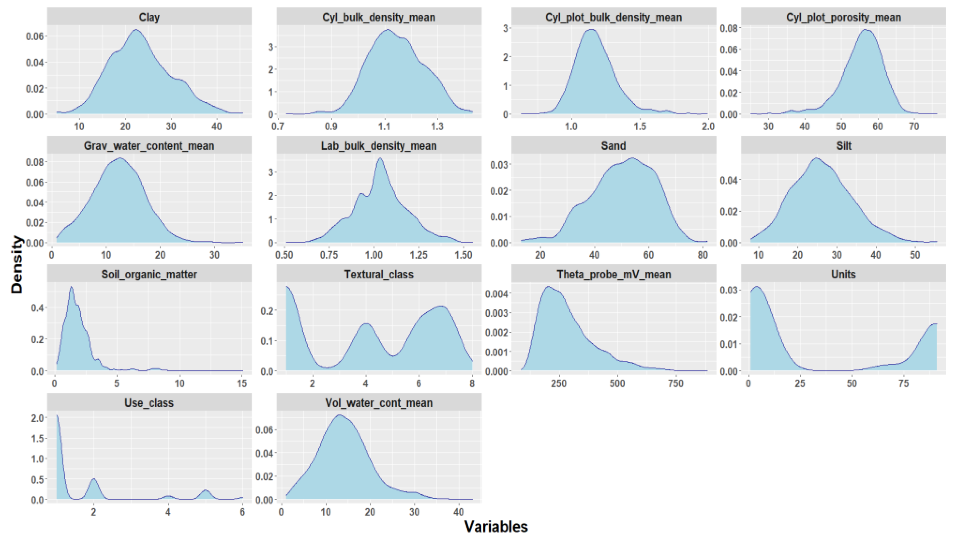
42]. The density plots of original data using the full data base are presented in
Figure 2. On the other hand,
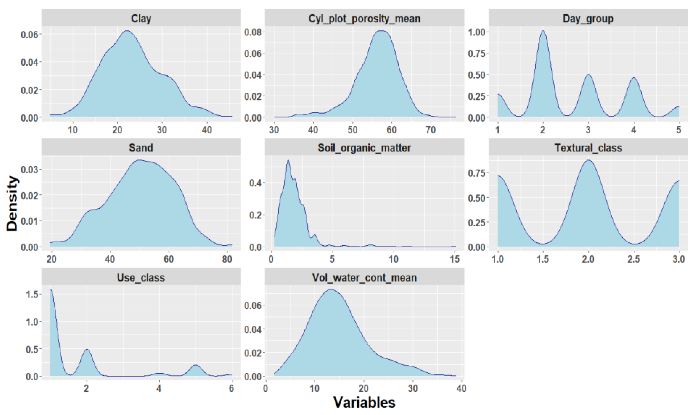
Figure 3 shows the same kind of plots, using the 848 rows of the data base with non missing data.
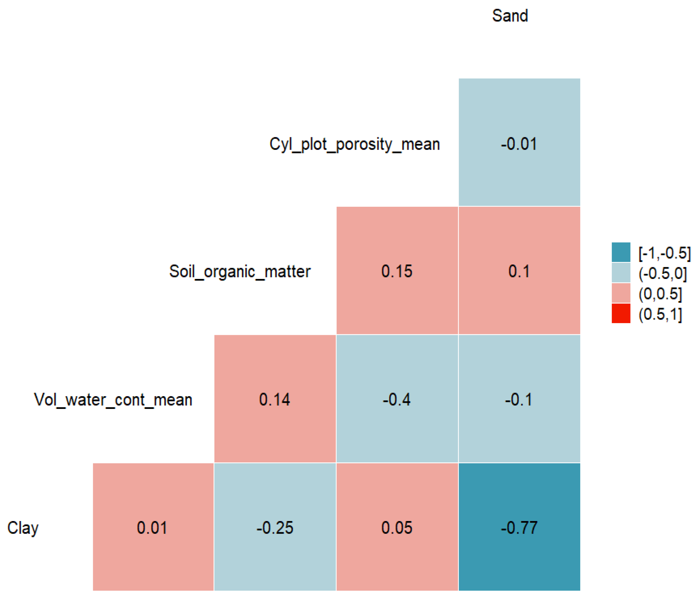
Figure 4 shows the correlation map between the continuous covariates in the study. In this figure, some of the cases are near 0.77 or −0.77 but most of them are not correlated, which is normal because of the data themselves have been processed without evaluating the temporal effect of Soil Moisture states.
In the soil, volumetric moisture content (θ m
3/m
3) is conditioned by the amount of water received as well as by the pressure with which it is retained in its pores. Depending on that pressure, soils can be in a state of saturation (θ
s), field capacity (θ
fc) or wilting point (θ
wp) [
38].
The time periods comprising the three campaigns studied were characterized by irregular rainfall which is typical of the Mediterranean climate. This particularity has permitted on the one hand, to analyze the most contrasting situations present in the study area: soil moisture values above field capacity (FC) and below the wilting point (WP). On the other hand, it has also permitted to evaluate different intermediate seasonal situations. The soil moisture dataset obtained for the different sampling days reveals the presence of significant differences of average moisture values.
Five different states of volumetric soil moisture were obtained in 6 selected days out of the 11 campaign days, namely: Very Wet (SM1, Day 3 in 2010) with mean values above FC (0.26 m
3/m
3); Wet (SM2, Days 1 and 2 in 2008) and Intermediate (SM3, Day 3 in 2008) with values between FC and WP (0.17–0.12 m
3/m
3); Dry (SM4, Day 4 in 2008) and Very Dry (SM5, Day 3 in 2009) with values (≤0,1 m
3/m
3) close to or lower than WP. These groups, characterized in
Table 1, show the different wetting/drying states that have been reached in the different campaigns.
The Very Wet (SM1) state average moisture value is above 0.25 m3/m3, since moisture values of that order are close to saturation (θs). Soils are considered Wet (SM2) when their values range between 0.25 and 0.15 m3/m3. These values are near or slightly above field capacity of the different soil types. The first and second days of 2008 (22 April and 24 April 2008) are grouped in this state since they present an average soil moisture value of 0.17 m3/m3 after registering accumulated precipitation of 45–60 mm the previous month in 2008, respectively.
The Intermediate (SM3) state represents the beginning of the soil-drying phase, and the corresponding values are between 0.10 and 0.15 m3/m3. This state, achieved in the area after a short period with no water intake, is presented on the third campaign day of 2008 (28 April) with mean soil moisture values of 0.12 m3/m3.
In the two following states the soil is dry, and the plant undergoes hydrological stress to a greater or lesser degree. The Dry state (SM4) presents moisture values near the wilting point with mean value of 0.096 m3/m3. This situation is typified on the fourth campaign day of 2008 (2 May 2008, the day furthest away from the last rainy event of the campaign).
The third day of 2009 (28 May 2009) corresponds to the Very Dry state (SM5), with moisture values of 0.05 m3/m3 that indicate a more advanced degree of dryness, with values overpassing the wilting point.
3.1. Soil Hydrodynamic Properties
Studies such as those carried out by [
43,
44,
45] suggest that soil properties at these scales are a major driver in soil moisture distribution and the detail of soil data leads to improving estimates of soil moisture.
The campaigns for SMOS validation provide a large number of measuring data acquired under different meteorological situations over time thus facilitating the analysis, infrequent, on seasonal variability of soil hydraulic properties [
46,
47] assuming the spatial homogeneity of climatic variables and a certain topographical uniformity and use in the VAS area, as indicated earlier.
3.1.1. Soil Textures
Textural analysis is one of the most useful soil variables to interpret the hydrological behavior of soils. 400 textures from the studied area have been used for this work. The textural classes that the area presents are sandy clay loam; loamy sand; loam and clay loam. This classification, according to the USDA textural triangle [
48], separates groups that induce the same properties in the soil with respect to soil structure, porosity and density, and therefore their hydrological behavior. To further explore these results, the textures have been grouped into three types depending on the percentage of their content in sand and clay. The established groups separate those with more than 20% clay whose textural class includes the qualification of “clayey” and those with more than 45% sand that includes the adjective “sandy”. These groups are: TX1 = % Clay <20% and predominant sand; TX2 and TX3: % Clay >20% if % Sand >45% is TX2 and if it is <45% TX3. If texture is contrasted versus moisture, the influence of this soil property will stand out in the higher or lower water retention capacity, as well as the significant effect of texture on moisture content according to the moisture state of the soil.
Throughout the different moisture states in which the soil can be found, it is verified that the soils included in Type TX1 (% Ac <20) have a lower SM value 0.25 ± 0.04 to 0.04 ± 0.01 m
3/m
3 than that registered by the other classes (TX2 = 0.26 ± 0.02 to 0.07 ± 0.02 m
3/m
3 and TX3 = 0.28 ± 0.04 to 0.05 ± 0.01 m
3/m
3), although it will not always be statistically significant) [
49]. In the area, the predominant particle size fraction in TX1 group is sand. The percent sand is related to the ability of a soil to drain quickly after rain events when the soil is still wet. The low stability of its aggregates and its single grain structure control the soil hydrological behavior. Due to this low water retention capacity in the soil, effective drainage and high infiltration rates are favored [
2]. The TX2 type with a percentage of clay >20% and sand >45% presents intermediate characteristics, so its behavior is close to class TX1 or class TX3 as a function of the different moisture states.
The results obtained when these textures with % Ac >20 predominate (TX2 and TX3) agree with other authors [
15,
16,
50], who related soil moisture content variability with variations in its texture. All of them confirmed that prevailing fine fraction corresponds to more duration of moist in time, as a consequence of structuring and creation of pore spaces of different sizes.
3.1.2. Porosity/Bulk Density
Bulk density (δ
bulk) is included within the minimum group of soil parameters to be measured as it is an indicator of the greater or lesser compaction and structure that it presents. Soil structure is a dynamic property and varies with the state of soil moisture. Changes in soil structure reflect changes in bulk density and, therefore, in its defined porosity ŋ = 1 − (δ
bulk/δ
real), where (ŋ) represents the total porosity. Interpreting data on total porosity (or bulk density) with respect to processes related to wetting or drying is complicated. The seasonal temporal variability [
24,
51] that characterizes this property is confirmed by the results since the mean values present significant differences when the hydrological conditions are very contrasting.
The Very Wet state (SM1) corresponds to the lowest porosity values (46%) and significantly different from those of other states (between 52% and 57%), since the soil aggregates can break or disperse and the pores compress or destroy, among other reasons, by rapid wetting of dry material or impact of the raindrop. On the contrary, the contraction of the soil when drying is one of the factors involved in the aggregation and formation of large pores [
52]. The soils in the area of study have Medium porosity (<50%) when they are very humid, going from Medium to High (50–60%) as the soil dries out. While the soil texture can be expected not to vary over time, soil structure and the geometry and volume of pores can be assumed to vary with season and weather [
47].
In states SM1 and SM2, coinciding with the periods in which the soil was wetter, a decreasing order of soil moisture is observed as porosity increases, with the least humid being the most porous.
In the SM5 state, the possibility of pore formation of all sizes and the appearance of drying cracks when the structural porosity is modified, induces an increment of porosity that permits to keep moisture longer, so that in these conditions, the more porous soils present the higher soil moisture [
51].
3.1.3. Soil Organic Matter and Land Use Influence
Another factor that influences water holding capacity is soil organic matter (SOM). The content of SOM is highly related to the degree and type of vegetation cover, so that the surface horizons of the soils under tillage contain smaller amounts than those that are under dense vegetation cover. The set of land uses of the area corresponding to this pixel of SMOS is characterized by presenting vineyards and to a lesser extent almond, olive, and cereal crops in the cultivated sector and in natural areas, shrubs with pine forests. For natural vegetation, mean values of SOM are above 4% and significantly different to that presented by the remaining land uses with organic matter content close to 2% or lower.
3.2. Soil Moisture Distribution to Pixel SMOS under Different Scenarios
Soil properties do not have a specific spatial continuity and their variability depends, among other things, on factors such as a drastic lithological change, according to a different geological material, or a change in use, caused by an anthropic transformation. Therefore, on the SMOS scale of work, executing ordinary kriging (OK) without interpolations between sampling points, is not easily conclusive. This is because the spatial representation of properties using estimates by adjusted distance metrics does not incorporate similarity in terms of quantifiable landscape characteristics [
53].
The subdivision of the SMOS pixel area in homogeneous units (SMOS units) allows to understand and spatially represent, with a systemic integral sense, the characteristics that determine its current environmental condition, especially the results of the properties of the soil that influence its moisture, facilitating the possibility of proposing scenarios that reflect different moistening situations [
54]. From the environmental SMOS units map delimited in the SMOS pixel of the VAS and the background of knowledge that has been acquired about the properties of the soil that determine its SM in a surface of more than 1000 km
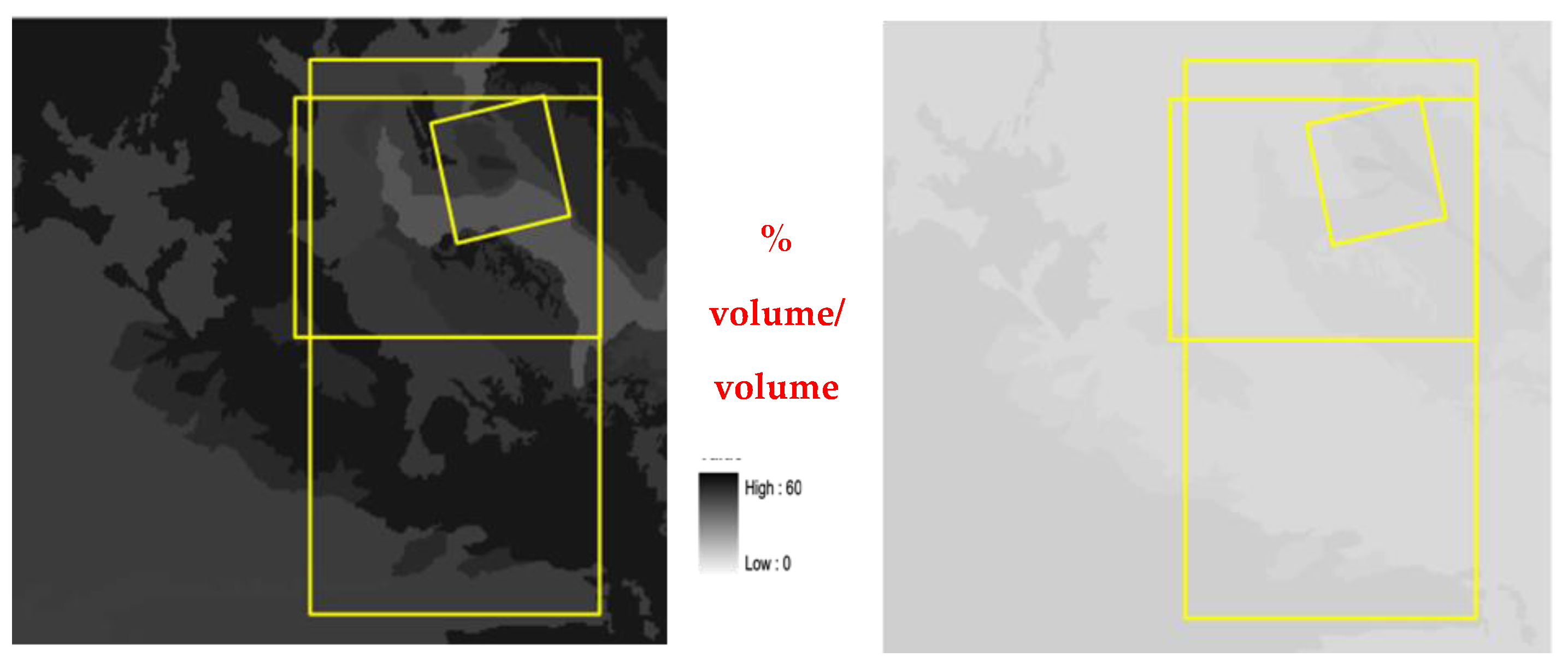
2 with the different campaigns of 2008, 2009 and 2010, a soil moisture proposal is made in the highest humidity and dry soil scenarios, by extrapolating the data acquired in the campaigns, to the entire SMOS pixel area (
Figure 5).
Maximum moisture at saturation conditions (θ
s) is estimated from minimum porosity data for that day assuming that all pores are filled with water. The wettest state observed in the three campaigns corresponds to the third day of the 2010 campaign classified as SM1. Under these conditions, porosity presents lower values since the structure is destroyed on wet floors with finer textures (
Figure 5 left).
Minimum moisture conditions are closed to the wilting point volumetric moisture (around 0.1 m
3/m
3) value. Volumetric moisture percentage at wilting point can be obtained from textural data. The parametric model used with satisfactory results for practical purposes [
55] is:
where θ
wp = Wilting point moisture percentage. Clay, silt and sand content are expressed in percentage. According to the textures analyzed, the average value of the wilting point percentage obtained for each delimited environmental unit varies between 13% and 9%, as depicted in
Figure 5 (right). In these conditions, the spatial variability of water content is minimal. Most of the plots corresponding to the soil moisture state typified as Dry (SM4) and all the soil samples corresponding to the Very Dry (SM5).
In the environmental units where data is lacking, their θ
wp and Moisture at saturation have been estimated by cartographic homologation with other units of environmental characteristics of land use, topography, and similar geological material assigning them the value obtained for their counterparts. On the one hand,
Figure 5 shows that the behavior of SMOS units in the maximum moistening states vary widely, showing the influence of land use and the hydrodynamic properties analyzed. On the other hand, the homogeneity of the data estimated for wilting point conditions is quite remarkable because since they do not register differences above 4%, they result significantly uniform for the measurements of a SMOS pixel. This proposal verifies the trend that environmental units under saturation conditions (SM1) with the lowest porosity are those that keep moisture in the wilting point, in the dry state. In the wettest stage, the soils with the highest moisture content are the least porous soils, reversing this trend in the less humid states where the most humid soils are kept the most porous.
3.3. Statistical Modelling
Linear models provide a simple way to relate a response variable with a set of covariates. In most observational studies as in our case, linear models are seriously affected by the presence of multicollinearity among the covariates included in them. In order to obtain a parsimonious model and to reduce the multicollinearity problem, we first performed a correlation analysis of the covariates and computed Generalized Variance Inflation Factors (GVIF) [
29,
56] to assess the presence of multicollinearity (
Table 2). GVIF were used to discard those covariates highly correlated with others. We used GVIF = 5 to assume that covariates above this threshold value are highly correlated and are thus non informative in the presence of others.
It is observed that there is a relationship between them. We propose, the next covariates and study these to include in the proposed model. The values of GVIF are presented in
Table 3.
In addition to the covariates selected, we include the spatial effect as a random effect, as well as time, in the model for soil moisture. To study the spatial effect, we use the mesh obtained by the SPDE method.
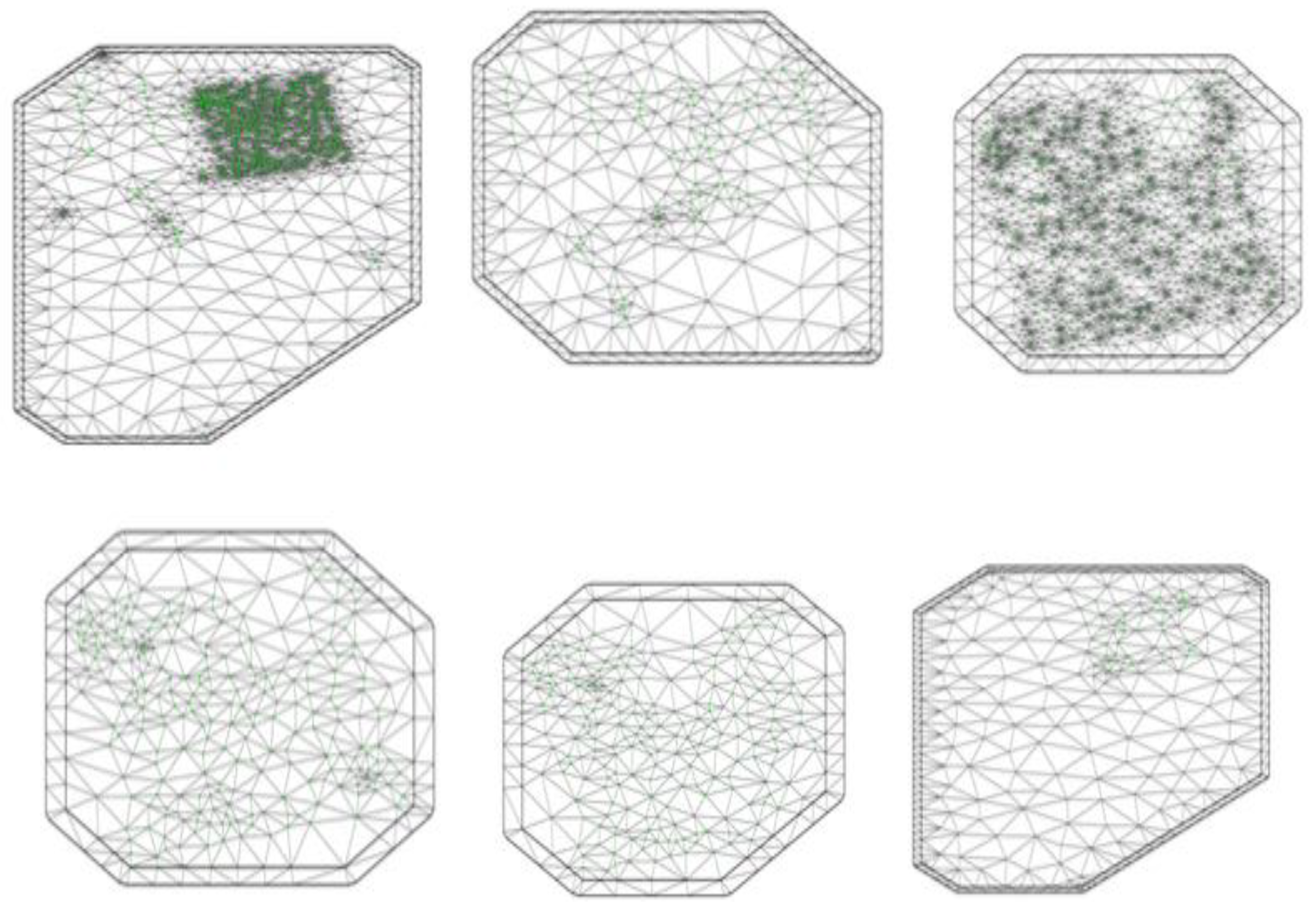
In
Figure 6, we present the meshes obtained for the fitting of the different models tested in this work. The inclusion of a spatial effect is important because the mesh is changing during the data days.
In
Table 4, the number of points and vertices is presented. The number of points and vertices in the mesh depend on the number of points sampled.
3.3.1. Statistical Models
We fitted a set of models that include the covariates plus a combination of spatial and temporal terms as random effects. The structure of the models fitted is shown in
Table 5.
Table 6 presents the summary statistics commonly used to assess the quality of the Bayesian models, for all the models fitted. According to the values in
Table 6, the best model is 2, since it has the lowest DIC value, in addition to a correlation coefficient close to 1 for the relationship between observed and predicted values and an associated error (RMSE) lower.
Figure 7 presents the scatter plot of the observed vs predicted values for model 2, showing a high correlation between the variables plotted. Model 2 describes soil moisture adequately and the predictions using this model under similar conditions to the ones included in the modeling process are reliable.
It is clearly observed that the correlation of models that include spatial and temporal random effects have a better fit according to
Table 5. With the results from model 2, we constructed Soil Moisture prediction maps as explained in next section.
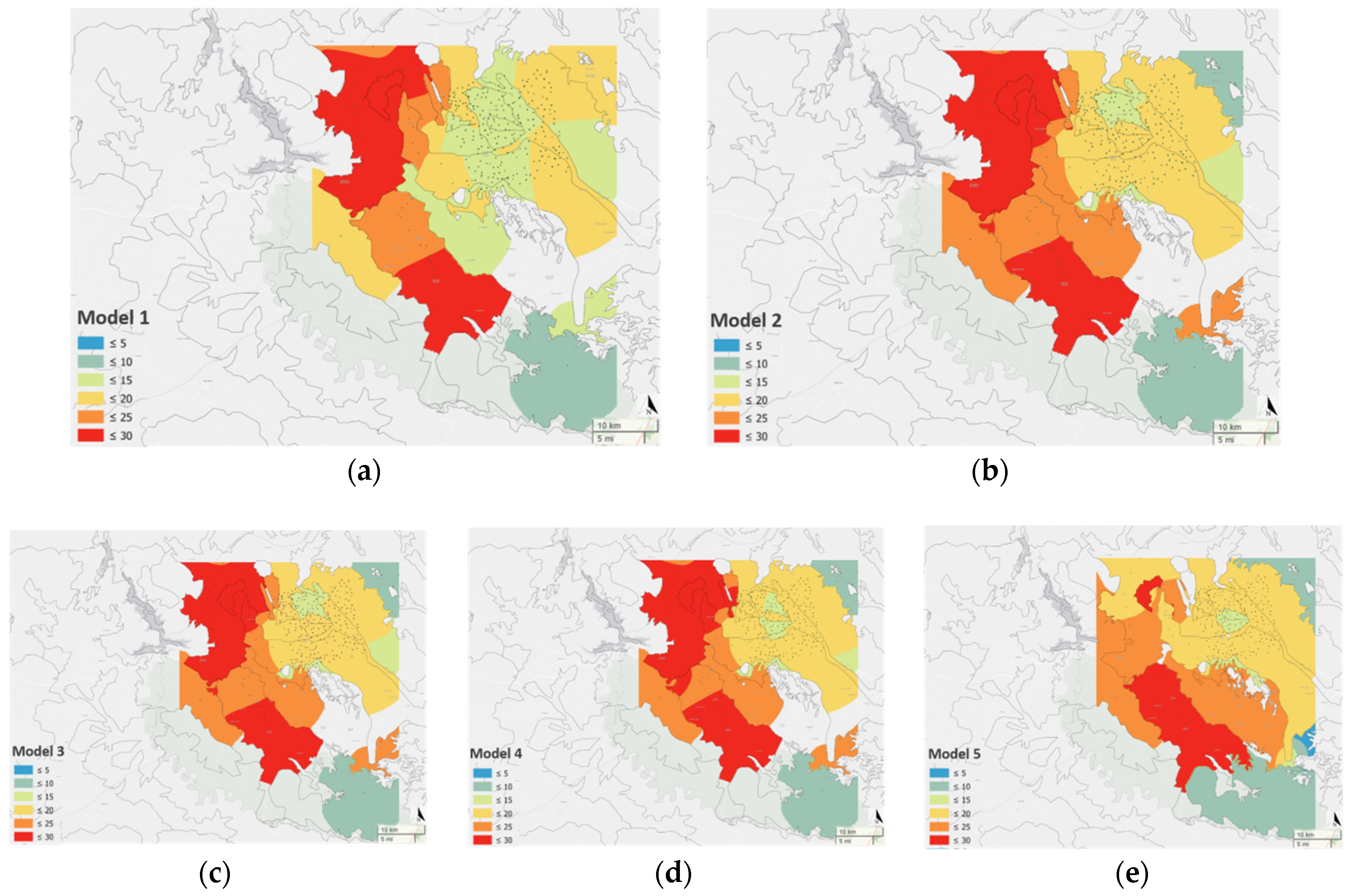
3.3.2. Spatial Prediction Maps
Soil moisture prediction maps are all presented in
Figure 8 and
Figure 9 are the same scale in order to make the results comparable.
Figure 8 shows the prediction maps obtained with each of the five models posted in
Table 5. The maps for models 2 to 5 look similar, but, according to
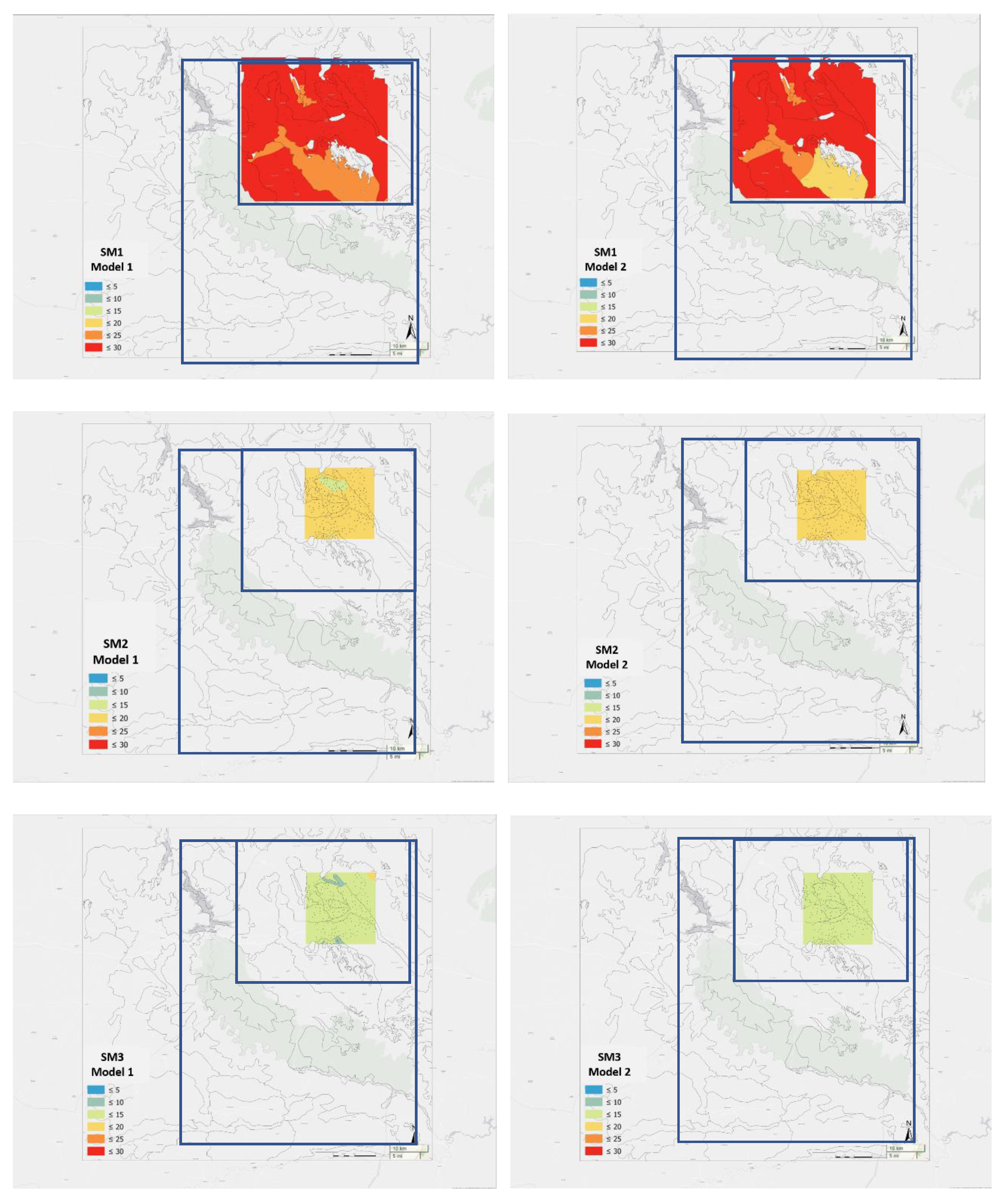
Table 5, it is model 2 the one that provided the best fit. Spatial predictions with model 1 look different but it should be noted that this model does not include temporal effect.
In order to show the changes of the spatial effect in soil moisture predictions across time, we obtained the prediction maps for SM states using model 2 but removing the temporal effect (model 1 in the plots, left panel) and removing the spatial and temporal effects (model 2 in the plots, right panel). The maps in
Figure 9 show differences by SM states and by model, justifying the need for the inclusion of spatial and temporal effects in soil moisture models, besides the inclusion of other covariates.
4. Discussion
The study of the data in VAS experimental site, during different days with different soil moisture conditions, is presented to help researchers in designing future sampling campaigns for soil moisture. In a typical analysis, for a covariate having values of the percentiles 0.025 and 0.975 with the same sign, indicates it is significant in the model. Regarding the different models for the different Soil Moisture states, a general pattern was detected where both porosity and organic matter are two significant elements in all the cases. The coefficients in the model increase for porosity and decrease for organic matter over time. Regarding the values obtained by the coefficients, it is worth noting the very high values of the SMOS Units factor and the texture factor as compared to the rest of the covariates used in the models. This makes it clear the need to work on soil moisture considering SMOS Units in the models, since they are not only significant but also have very large coefficients, about 10 times larger than other variables.
It is worth mentioning that although not all the covariates in the models are significant, their inclusion contributes to reduce the DIC and improves model fitting. This non-significance of some covariates in the models is a consequence of the multicollinearity observed in the covariates.
5. Conclusions
We have presented here the results of the spatial and temporal analysis of soil moisture data used to calibrate their values through the SMOS campaigns.
The use of the INLA-SPDE methodology used here has allowed us to fit spatial and temporal hierarchical models that are too complicated to be fitted by maximum likelihood methods. The models allow to analyze the effects of covariates related to soil moisture filtering out the effect of spatial and temporal variation. Moreover, the use of this methodology permits to design more efficient sampling campaigns for future SMOS missions. In addition, it also allows to construct soil moisture maps in a more sensible and efficient way. The models fitted show the advantage of the inclusion of covariates and the SMOS units to analyze soil moisture of an area.
Although the process of sampling, descriptive analysis, selection of covariates, modeling and creation of prediction maps is long, it is necessary in order to show that the SMOS mission facilitates the study of large areas with simpler samples and that the INLA-SPDE methodology is very efficient in this type of modeling with a large amount of data and affected covariates.
Author Contributions
Conceptualization, E.C., P.J. and C.A.; Data curation, E.C., P.J., C.A. and S.C.; Formal analysis, P.J., E.C., C.A. and S.C.; Methodology, E.C., P.J., C.A., E.L.-B. and C.D.-A.; Project administration, E.L.-B., E.C., P.J. and C.A.; Resources, E.C., C.A. and E.L.-B.; Software, P.J. and S.C.; Validation, E.L.-B. and C.D.-A.; Writing—original draft, E.C., P.J. and C.A.; Writing review & editing, C.D.-A., E.L.-B. and S.C. All authors have read and agreed to the published version of the manuscript.
Funding
This research received no external funding.
Acknowledgments
This work has been carried out in the framework of the projects (i) Validation of SMOS Products over Mediterranean Ecosystem Vegetation at the Valencia Anchor Station Reference Area. ESA SMOS Cal/Val A.O. ID 3252 Agreement of Collaboration, (ii) Soil Moisture Changes as a Function of Natural and Anthropic Edaphic Parameters. Use of SMOS Calibration/Validation Products from the Education Department of the Regional Government of Valencia (iii) MIDAS-5. Product Validation, Data Exploitation and Expert Center for the SMOS Mission. UVEG Part (MIDAS-5/UVEG) (Spanish Ministry for Science and Innovation) and (iv) MIDAS-6. SMOS Ocean Salinity and Soil Moisture Products. Improvements and Applications Demonstration. UVEG Part (MIDAS-5/UVEG) (Spanish Ministry for Economy and Competitiveness).
Conflicts of Interest
The authors declare that they have no known competing financial interests or personal relationships which have, or could be perceived to have, influenced the work reported in this article.
References
- Mälicke, M.; Hassler, S.K.; Blume, T.; Weiler, M.; Zehe, E. Soil moisture: Variable in space but redundant in time. Hydrol. Earth Syst. Sci. 2020, 24, 2633–2653. [Google Scholar] [CrossRef]
- Ceballos, A.; Martínez-Fernández, J.; Santos, F.; Alonso, P. Soil-water behaviour of sandy soils under semi-arid conditions in the Duero Basin (Spain). J. Arid Environ. 2002, 51, 501–519. [Google Scholar] [CrossRef]
- Castillo, E.; Castellví, F. Agrometeorología; Mundi Prensa: Madrid, Spain, 2001. [Google Scholar]
- Bosch, D.D.; Lakshmi, V.; Jackson, T.J.; Choi, M.; Jacobs, J.M. Large scale measurements of soil moisture for validation of remotely sensed data: Georgia soil moisture experiment of 2003. J. Hydrol. 2006, 323, 120–137. [Google Scholar] [CrossRef]
- Kerr, Y.H. Soil moisture from space: Where are we? Hydrogeol. J. 2007, 15, 117–120. [Google Scholar] [CrossRef]
- Brocca, L.; Ciabatta, L.; Massari, C.; Camici, S.; Tarpanelli, A. Soil moisture for hydrological applications: Open questions and new opportunities. Water 2017, 9, 140. [Google Scholar] [CrossRef]
- Pezij, M.; Augustijn, D.C.M.; Hendriks, D.M.D.; Hulscher, S.J.M.H. Applying transfer function-noise modelling to characterize soil moisture dynamics: A data-driven approach using remote sensing data. Environ. Modell. Softw. 2020, 131, 104756. [Google Scholar] [CrossRef]
- Kerr, Y.H.; Waldteufel, P.; Wigneron, J.-P.; Font, J.; Berger, M. Soil moisture retrieval from space: The Soil Moisture and Ocean Salinity (SMOS) mission. IEEE T. Geosci. Remote 2001, 39, 1729–1735. [Google Scholar] [CrossRef]
- Kerr, Y.; Waldteufel, P.; Wigneron, J.; Delwart, S.; Cabot, F.; Boutin, J.; Escorihuela, M.; Font, J.; Reul, N.; Gruhier, C.; et al. The SMOS Mission: New Tool for Monitoring Key Elements of the Global Water Cycle. Proc. IEEE 2010, 98, 666–687. [Google Scholar] [CrossRef] [Green Version]
- Wigneron, J.-P.; Li, X.; Frappart, F.; Fan, L.; Al-Yaari, A.; De Lannoy, G.; Liu, X.; Wang, M.; Le Masson, E.; Moisy, C. SMOS-IC data record of soil moisture and L-VOD: Historical development, applications and perspectives. Remote Sens. Environ. 2021, 254, 112238. [Google Scholar] [CrossRef]
- López-Baeza, E.; Antolñin Tomás, M.C. Validation of SMOS Products over Mediterranean Ecosystem Vegetation at the Valencia Anchor Station Reference Area; Desertification Research Centre: Moncada, Spain, 2006. [Google Scholar]
- Juglea, S.; Kerr, Y.; Mialon, A.; Wigneron, J.-P.; Lopez-Baeza, E.; Cano, A.; Albitar, A.; Millan-Scheiding, C.; Antolin, C.; Delwart, S. Modelling Soil Moisture at SMOS Scale by Use of a SVAT Model over the Valencia Anchor Station. Hydrol. Earth Syst. Sci. 2010, 14, 831–846. [Google Scholar] [CrossRef] [Green Version]
- Juglea, S.; Kerr, Y.; Mialon, A.; López-Baeza, E.; Braithwaite, D.; Hsu, K. Evaluation of PERSIANN Database in the Framework of SMOS Calibration/Validation Activities over Valencia Anchor Station. Hydrol. Earth Syst. Sci. 2010, 14, 1509–1525. [Google Scholar] [CrossRef] [Green Version]
- Delwart, S.; Bouzinac, C.; Wursteisen, P.; Berger, M.; Drinkwater, M.; Martin-Neira, M.; Kerr, Y. SMOS validation and the COSMOS campaigns. IEEE T. Geosci. Remote 2008, 46, 695–704. [Google Scholar] [CrossRef]
- Famiglietti, J.S.; Rudnicki, J.W.; Rodell, M. Variability in surface moisture content along a hillslope transect: Rattlesnake Hill, Texas. J. Hydrol. 1998, 210, 259–281. [Google Scholar] [CrossRef] [Green Version]
- Gómez-Plaza, A.; Martínez-Mena, M.; Albadalejo, J.; Castillo, V. Factors regulating spatial distribution of soil water content in small semiarid catchments. J. Hydrol. 2001, 253, 211–226. [Google Scholar] [CrossRef]
- Lekshmi-Su, S.; Singh, D.N.; Baghini, M.S. A critical review of soil moisture measurement. Measurement 2004, 54, 92–105. [Google Scholar]
- Entin, J.K.; Robock, A.; Vinnikov, K.Y.; Hollinger, S.E.; Liu, S.; Namkhai, A. Temporal and spatial scales of observed soil moisture variations in the extratropics. J. Geophys. Res. 2000, 105, 11865–11877. [Google Scholar] [CrossRef]
- Millán-Scheiding, C.; Antolín, C.; Cano, A.; López-Baeza, E. Uso de Unidades Fisio-Hidrológicas en la Monitorización de la Humedad del Suelo con SMOS. In Proceedings of the III Simposio Nacional sobre Control de la Degradación de Suelos y la Desertificación, Fuerteventura, Spain, 16–20 September 2007; pp. 51–52. [Google Scholar]
- Millán-Scheiding, C.; Antolín, C.; Marco, J.; Soriano, M.P.; Torre, E.E.; Requena, F.; Carbó, E.E.; Cano, A.; López-Baeza, E. Use of physio-hydrological units for SMOS validation at the Valencia Anchor Station study area. In Abstracts of the European Geosciences Union; European Geoscience Union: Vienna, Austria, 2009. [Google Scholar]
- Antolín, M.C.; The CAROLS@VAS Team. Ground Sampling Strategy and Measurements during the CNES CAROLS Campaign at the Valencia Anchor Station. In Abstracts of the European Geosciences Union; European Geoscience Union: Vienna, Austria, 2010. [Google Scholar]
- Antolín Tomás, C.; Millán-Scheiding, C.; López-Baeza, E.; Requena Tierno, F.; Torre Fernández, E.; Carbó Valverde, E. Distribución de la humedad del suelo en las unidades ambientales de la campaña CNES-CAROLS 2010 (SMOS) y su relación con los usos del suelo. In Proceedings of the V Simposio Nacional Sobre Control de la Degradación y uso Sostenible del Suelo, Murcia, Spain, 27–30 June 2011; pp. 463–467. [Google Scholar]
- Santanello, J.A., Jr.; Peters-Lidard, C.; Garcia, M.; Mocko, D.; Tischler, M.A.; Moran, S.; Homa, T.D.P. Using remotely-sensed estimates of soil moisture to infer soil texture and hydraulic properties across a semi-arid watershed. Remote Sens. Environ. 2007, 110, 79–97. [Google Scholar] [CrossRef] [Green Version]
- Givi, J.; Prasher, S.O.; Patel, R.M. Evaluation of pedotransfer functions in predicting the soil water contents at field capacity and wilting point. Agr. Water Manag. 2004, 70, 83–96. [Google Scholar] [CrossRef]
- Rue, H.; Martino, S.; Chopin, N. Approximate Bayesian inference for latent Gaussian models using integrated nested Laplace approximations (with discussion). J. R. Stat. Soc. B. 2009, 71, 319–392. [Google Scholar] [CrossRef]
- Lindgren, F.; Rue, H.; Lindstrom, J. An explicit link between Gaussian fields and Gaussian Markov random fields the SPDE approach. J. R. Stat. Soc. B. 2011, 423–498. [Google Scholar] [CrossRef] [Green Version]
- Sun, X.-L.; Minasny, B.; Wang, H.-L.; Zhao, Y.-G.; Zhang, G.-L.; Wu, Y.-J. Spatiotemporal modelling of soil organic matter changes in Jiangsu, China between 1980 and 2006 using INLA-SPDE. Geoderma 2020, 384, 114808. [Google Scholar] [CrossRef]
- Juan Verdoy, P. Enhancing the SPDE modeling of spatial point processes with INLA, applied to wildfires. Choosing the best mesh for each database. Commun. Stat. Simulat. 2019, 1–34. [Google Scholar] [CrossRef]
- Juan Verdoy, P. Spatio-temporal hierarchical Bayesian analysis of wildfires with Stochastic Partial Differential Equations. A case study from Valencian Community (Spain). J. Appl. Stat. 2020, 47, 927–946. [Google Scholar] [CrossRef]
- Pérez Cueva, A. Atlas Climático de la Comunidad Valenciana (1961–1990); COPUT, Generalitat Valenciana: Valencia, Spain, 1994. [Google Scholar]
- López-Baeza, E.; SMOS Cal/Val AO Project No.3252 Team. Valencia Site Data Processing & Model Results; Workshop of the SMOS Validation Rehearsal Campaign NH Conference Centre Leeuwenhorst: Noordwijkerhout, The Netherlands, 2008. [Google Scholar]
- López-Baeza, E.; Antolín, M.C.; Balling, F.; Belda, C.; Bouzinac, F.; Camacho, A.; Cano, E.; Carbo, S.; Delwart, C.; Domenech, A.G.; et al. Wursteisen. Soil moisture characterization of the Valencia Anchor Station. Ground, Aircraft Measurements and simulations. In Proceedings of the 2nd EPS/Metop RAO Workshop European Space Agency, Barcelona, Spain, 20–22 May 2009. [Google Scholar]
- López-Baeza, E.; Acosta, R.; Antolín, M.C.; Balling, J.; Belda, F.; Bouzinac, C.; Cano, A.; Delwart, S.; Domenech, C.; Ferreira, A.G.; et al. Validation Activities Preparation for SMOS (Soil Moisture and J.-P. Ocean Salinity) Land Products at the Valencia Anchor Station. In Proceedings of the EUMETSAT Meteorological Satellite Conference, Darmstadt, Germany, 8–12 September 2008. [Google Scholar]
- López-Baeza, E.; Antolín, C.; Belda, A.; Cano, A.; Camps, A.; Fidalgo, B.; Martínez, C.; Millán, C.; Sanchis, J.; Vall-Ilosera, M. SMOS Validation Pixel. Scheme for Cal/Val Activities. The Valencia Anchor Station Site; SMOS Cal/Val Workshop: Frascati, Italy, 2007. [Google Scholar]
- López-Baeza, E.; Antolín Tomás, C.; Bouzinac, C.; del Álamo, C.; Davidson, M.; Drusch, M.; Herrero Isern, J.; Juglea, S.; Kerr Yann, H.; Mecklenburg, S.; et al. CNES and ESA CAROLS Airborne Campaigns at the Valencia Anchor Station and Los Monegros Site in the Framework of SMOS Validation. In Abstracts of the European Geosciences Union; European Geoscience Union: Vienna, Austria, 2011. [Google Scholar]
- Saleh, K.; López-Baeza, E.; Cano, A.; Millán-Scheiding, C.; Antolín, C.; SMOS Validation Rehearsal Team. SMOS Meeting. In Proceedings of the SMOS Validation Rehearsal Flights (EMIRAD) Valencia, Bordeaux, France, 30–31 October 2008. [Google Scholar]
- Saleh, K.; López-Baeza, E.; Millán-Scheiding, C.; Antolín, C.; Juglea, S.; Wigneron, J.-P.; Keer, Y.; SMOS Rehearsal Team. Soil moisture estimates from the SMOS Validation rehearsal campaign at the Valencia site. In Abstracts of the European Geosciences Union; European Geoscience Union: Vienna, Austria, 2008. [Google Scholar]
- Porta, J.; López-Acevedo, M.; Rodríguez, R. Técnicas y Experimentos en Edafología; Colegio de Ingenieros Agrónomos de Cataluña: Barcelona, Spain, 1986. [Google Scholar]
- MAPA. Métodos Oficiales de Análisis de Suelos y Aguas; Ministerio de Agricultura, Pesca y Alimentación: Madrid, Spain, 1994. [Google Scholar]
- The R Core Team. R: A Language and Environment for Statistical Computing; R Foundation for Statistical Computing: Vienna, Austria, 2016. [Google Scholar]
- R-INLA Project. Available online: http://www.r-inla.org/home (accessed on 5 November 2019).
- Carbó, E.; Antolín, C.; Millán-Scheiding, C.; Requena, F.; Torre, E. Análisis de variables edáficas relacionadas con la humedad del suelo en unidades fisio-hidrológicas utilizadas para la cal/val de SMOS en el área de la Valencian Anchor Station (VAS). In Proceedings of the IV Simposio Nacional sobre Control de la Degradación de los Suelos y Cambio Global, Valencia, Spain, 8–11 September 2009; pp. 223–224. [Google Scholar]
- Crave, A.; Gascuel-Odoux, C. The influence of topography on time and space distribution of soil surface water content. Hydrol. Process. 1997, II, 203–210. [Google Scholar] [CrossRef]
- Buttafuoco, G.; Castrignano, A.; Busoni, E.; Dimase, A.C. Studying the spatial structure evolution of soil water content using multivariate geostatistics. J. Hydrol. 2005, 311, 202–218. [Google Scholar] [CrossRef]
- Baggaley, N.; Mayr, T.; Bellamy, P. Identification of key soil and terrain properties that influence the spatial variability of soil moisture throughout the growing season. Soil Use Manag. 2009, 25, 262–273. [Google Scholar] [CrossRef]
- Lin, H.S.; Kogelmann, W.; Walker, C.; Bruns, M.A. Soil moisture patterns in a forested catchment: A hydropedological perspective. Geoderma 2006, 131, 345–368. [Google Scholar] [CrossRef]
- Bormann, H.; Klaassen, K. Seasonal and land use dependent variability of soil hydraulic and soil hydrological properties of two Northern German soils. Geoderma 2008, 145, 295–302. [Google Scholar] [CrossRef]
- Soil Survey Staff. Soil Survey Laboratory Methods Manual, 3rd ed.; Report 42; USDA—Natural Resources Conservation Service, National Soil Survey Center: Lincoln, NE, USA, 1996.
- Mentges, M.I.; Reichert, J.M.; Rodrigues, M.F.; Awe, G.O.; Mentges, L.R. Capacity and intensity soil aeration properties affected by granulometry, moisture, and structure in no-tillage soils. Geoderma 2016, 263, 47–59. [Google Scholar] [CrossRef]
- Kar, G.; Kumar, A.; Singh, R. Spatial distribution of soil hydro-physical properties and morphometric analysis of rainfed watershed as a tool for sustainable land use planning. Agr. Water Manag. 2009, 96, 1449–1459. [Google Scholar] [CrossRef]
- Alletto, L.; Coquet, Y. Temporal and spatial variability of soil bulk density and near-saturated hydraulic conductivity under two contrasted tillage management systems. Geoderma 2009, 152, 85–94. [Google Scholar] [CrossRef]
- Gregory, P.J. El Agua y el Crecimiento de los Cultivos. In Condiciones del Suelo y Desarrollo de las Plantas Según Russell; Mundi Prensa Ed.: Madrid, Spain, 1992; pp. 355–395. [Google Scholar]
- Lyon, S.W.; Sørensen, R.; Stendah, J.; Seibert, J. Using landscape characteristics to define an adjusted distance metric for improving kriging interpolations. IJGIS 2010, 24, 723–740. [Google Scholar] [CrossRef] [Green Version]
- Martínez, G.; López Blanco, J. Caracterización de las unidades ambientales biofísicas del Glacís de Buenavista, Morelos, mediante la aplicación del enfoque geomorfológico morfogenético. Investig. Geográficas 2005, 58, 34–53. [Google Scholar] [CrossRef]
- Fuentes, J.L. Técnicas de Riego, 4th ed.; Mundi Prensa Ed.: Madrid, Spain, 2003. [Google Scholar]
- Carbó, E.; Juan, P.; Añó, C.; Antolín, C. Modelización de propiedades del suelo que influyen en su humedad. In Proceedings of the IX Simposio Nacional Sobre Control de la Degradación y Recuperación de Suelos, Elche, Spain, 24–25 May 2021; pp. 121–128. [Google Scholar]
Figure 1.
Study area with detailed physio-hydrological units. Area of the field campaigns highlighted in yellow (2008), brown (2009) and green (2010).
Figure 1.
Study area with detailed physio-hydrological units. Area of the field campaigns highlighted in yellow (2008), brown (2009) and green (2010).
Figure 2.
Density plot of original data. Theta probe mV mean (mV), Volumetric water content mean (%), Gravimetric water content mean (%), Laboratory bulk density mean (g cm−3), Cylinder bulk density mean (g cm−3), Cylinder plot bulk density mean (g cm−3), Cylinder plot porosity mean (%), Soil organic matter (%), Sand (%), Silt (%), Clay (%).
Figure 3.
Density plot of variables used in designing the models (selected variables).
Figure 3.
Density plot of variables used in designing the models (selected variables).
Figure 4.
Mutual correlation values among response variable and covariates used in the models.
Figure 4.
Mutual correlation values among response variable and covariates used in the models.
Figure 5.
Proposal of soil moisture (%) distribution for a SMOS pixel under maximum (left) and minimum (right) soil moisture conditions. Unit in % volume/volume represents volume of water per total volume of soil.
Figure 5.
Proposal of soil moisture (%) distribution for a SMOS pixel under maximum (left) and minimum (right) soil moisture conditions. Unit in % volume/volume represents volume of water per total volume of soil.
Figure 6.
Stochastic Partial Differential Equation (SPDE) meshes for spatial study. Top line, from left to right every study day, day 1 and day 2. Bottom line, from left to right days 3 to 5. The sample points are highlighted in green.
Figure 6.
Stochastic Partial Differential Equation (SPDE) meshes for spatial study. Top line, from left to right every study day, day 1 and day 2. Bottom line, from left to right days 3 to 5. The sample points are highlighted in green.
Figure 7.
Scatter plot of model 2, observed vs. predicted (soil moisture content in %).
Figure 7.
Scatter plot of model 2, observed vs. predicted (soil moisture content in %).
Figure 8.
Prediction maps from model 1 (a) to model 5 (e). depicting soil moisture content in %.
Figure 8.
Prediction maps from model 1 (a) to model 5 (e). depicting soil moisture content in %.
Figure 9.
Prediction maps for Soil Moisture states (SM 1 to 3) for model 1 (left) model 2 (right).
Figure 9.
Prediction maps for Soil Moisture states (SM 1 to 3) for model 1 (left) model 2 (right).
Table 1.
Mean value of five volumetric soil moisture states.
Table 1.
Mean value of five volumetric soil moisture states.
| SM | SM1 | SM2 | SM3 | SM4 | SM5 |
|---|
| θ (m3/m3) | 0.26 ± 0.04 | 0.17 ± 0.03 | 0.12 ± 0.03 | 0.10 ± 0.03 | 0.05 ± 0.03 |
| | n:230 | n:1245 | n:614 | n:569 | n:245 |
Table 2.
Generalized Variance Inflation Factors (GVIF) values of all variables.
Table 2.
Generalized Variance Inflation Factors (GVIF) values of all variables.
| Variable | GVIF |
|---|
| Theta Probe mV mean | 1.3772 |
| Volumetric water content mean | 79.2841 |
| Gravimetric water content mean | 60.9323 |
| Laboratory Bulk Density mean | 6445.0208 |
| Cylinder Bulk Density mean | 30,799.7735 |
| Cylinder Plot Bulk Density mean | 4485.6053 |
| Soil organic matter | 1.5845 |
| Sand | 15,770.7005 |
| Silt | 6877.5390 |
| Clay | 5858.6278 |
| Textural class | 3.8870 |
| Land use class | 1.3824 |
| SMOS Units | 1.4977 |
Table 3.
Generalized Variance Inflation Factors (GVIF) values of selected variables.
Table 3.
Generalized Variance Inflation Factors (GVIF) values of selected variables.
| Variable | GVIF |
|---|
| Textural class | 3.7495 |
| Volumetric water content mean | 1.2838 |
| Cylinder plot porosity mean | 1.3188 |
| Soil organic matter | 1.4125 |
| Sand | 3.1841 |
| Clay | 3.7679 |
| Land use class | 1.3106 |
| SMOS Units | 1.1298 |
Table 4.
Number of points and vertices for individual mesh used in the models.
Table 4.
Number of points and vertices for individual mesh used in the models.
| SM | SM ALL | SM1 | SM2 | SM3 | SM4 | SM5 |
|---|
| Points | 1020 | 116 | 435 | 215 | 199 | 55 |
| Vertex | 9357 | 413 | 5146 | 367 | 398 | 406 |
Table 5.
Overview of model structure.
Table 5.
Overview of model structure.
| Model | Spatial Effect | Temporal Effect Random Walk Type1 | Cylinders Plot Porosity Mean | Soil
Organic Matter | Sand | Clay | Textural Class | Land Use | SMOS
Unit | Temporal Effect-Day |
|---|
| 1 | x | | x | x | x | x | x | x | x | |
| 2 | x | | x | x | x | x | x | x | x | x |
| 3 | | | x | x | x | x | x | x | x | x |
| 4 | x | x | x | x | x | x | x | x | x | |
| 5 | | x | x | x | x | x | x | x | x | |
Table 6.
Review and comparison of model results.
Table 6.
Review and comparison of model results.
| | Model 1 | Model 2 | Model 3 | Model 4 | Model 5 |
|---|
| DIC | 6254.85 | 4817.06 | 5060.36 | 4817.67 | 5060.39 |
| Correlation | 0.5842 | 0.9357 | 0.8879 | 0.9355 | 0.8879 |
| RMSE | 4.96 | 2.16 | 2.81 | 2.16 | 2.81 |
| Publisher’s Note: MDPI stays neutral with regard to jurisdictional claims in published maps and institutional affiliations. |
© 2021 by the authors. Licensee MDPI, Basel, Switzerland. This article is an open access article distributed under the terms and conditions of the Creative Commons Attribution (CC BY) license (https://creativecommons.org/licenses/by/4.0/).


 ,
, 


