
A Comparison of UAV RGB and Multispectral Imaging in Phenotyping for Stay Green of Wheat Population

1
College of Mechanical and Electronic Engineering, Northwest A & F University, Yangling 712100, China
2
Key Laboratory of Agricultural Internet of Things, Ministry of Agriculture and Rural Affairs, Northwest A & F University, Yangling 712100, China
3
Shaanxi Key Laboratory of Agricultural Information Perception and Intelligent Service, Northwest A & F University, Yangling 712100, China
4
College of Agronomy, Northwest A & F University, Yangling 712100, China
5
State Key Laboratory of Crop Stress Biology for Arid Areas, Northwest A & F University, Yangling 712100, China
*
Author to whom correspondence should be addressed.
Remote Sens. 2021, 13(24), 5173; https://0-doi-org.brum.beds.ac.uk/10.3390/rs13245173
Submission received: 9 November 2021
/
Revised: 11 December 2021
/
Accepted: 16 December 2021
/
Published: 20 December 2021
(This article belongs to the Section Remote Sensing in Agriculture and Vegetation)
Abstract
:High throughput phenotyping (HTP) for wheat (Triticum aestivum L.) stay green (SG) is expected in field breeding as SG is a beneficial phenotype for wheat high yield and environment adaptability. The RGB and multispectral imaging based on the unmanned aerial vehicle (UAV) are widely popular multi-purpose HTP platforms for crops in the field. The purpose of this study was to compare the potential of UAV RGB and multispectral images (MSI) in SG phenotyping of diversified wheat germplasm. The multi-temporal images of 450 samples (406 wheat genotypes) were obtained and the color indices (CIs) from RGB and MSI and spectral indices (SIs) from MSI were extracted, respectively. The four indices (CIs in RGB, CIs in MSI, SIs in MSI, and CIs + SIs in MSI) were used to detect four SG stages, respectively, by machine learning classifiers. Then, all indices’ dynamics were analyzed and the indices that varied monotonously and significantly were chosen to calculate wheat temporal stay green rates (SGR) to quantify the SG in diverse genotypes. The correlations between indices’ SGR and wheat yield were assessed and the dynamics of some indices’ SGR with different yield correlations were tracked in three visual observed SG grades samples. In SG stage detection, classifiers best average accuracy reached 93.20–98.60% and 93.80–98.80% in train and test set, respectively, and the SIs containing red edge or near-infrared band were more effective than the CIs calculated only by visible bands. Indices’ temporal SGR could quantify SG changes on a population level, but showed some differences in the correlation with yield and in tracking visual SG grades samples. In SIs, the SGR of Normalized Difference Red-edge Index (NDRE), Red-edge Chlorophyll Index (CIRE), and Normalized Difference Vegetation Index (NDVI) in MSI showed high correlations with yield and could track visual SG grades at an earlier stage of grain filling. In CIs, the SGR of Normalized Green Red Difference Index (NGRDI), the Green Leaf Index (GLI) in RGB and MSI showed low correlations with yield and could only track visual SG grades at late grain filling stage and that of Norm Red (NormR) in RGB images failed to track visual SG grades. This study preliminarily confirms the MSI is more available and reliable than RGB in phenotyping for wheat SG. The index-based SGR in this study could act as HTP reference solutions for SG in diversified wheat genotypes.
1. Introduction
Wheat (Triticum aestivum L.) is a widely cultivated and consumed cereal crop globally and breeding varieties with high and stable yields could reduce population growth and climate changes pressure [1,2]. Wheat yield mainly comes from canopy organ (leaf and spike) photosynthesis during the grain filling stage. It is generally considered an effective way to improve wheat yield by delaying wheat canopy organ senescence to maintain strong photosynthetic capacity and provide more assimilates. The trait of delaying senescence and prolonging canopy vigor in the late growth stage is called stay green (SG) [3,4,5]. In addition, SG is a beneficial phenotype to wheat adaptability to abiotic stresses such as drought, heat, salinity, and other environmental factors [6,7,8]. Therefore, breeding new wheat varieties with excellent SG is an approved target, and phenotyping for SG is also an indispensable task in high-yield and stress-resistance breeding. Wheat SG changes mainly occur from the anthesis to the maturity stage, followed by stem and leaf greenness fading and spike and grain maturity. However, wheat stay green is a complex biological phenomenon or dynamic quantitative trait, which is affected by multiple environmental factors, complicated genetic mechanisms, diversified senescence patterns, and changes in microscopic biochemical components during late development [9,10,11]. For wheat SG, precision screening and identification are difficult to achieve by traditional phenotyping methods (visual scoring, physiological and biochemical trait measurement, etc.) with great subjective influence and disadvantages of being time consuming and laborious in natural populations in the field. In this case, a large number of diversified genotypes are usually planted in hundreds of plots. Furthermore, high throughput gene sequencing technology has made it easy to obtain high-density gene markers. However, the lack of matched high-throughput phenotype data is still a bottleneck for natural population genome-wide association analysis (GWAS) to mining excellent genes [12,13]. High throughput phenotyping technologies, which aim to obtain crop phenotypes quickly and repeatedly, have received more attention and have been applied to bridge the gap between genotypes and phenotypes [14,15,16]. For field crops, unmanned aerial vehicle (UAV) multispectral and low-cost RGB (red, green, blue) imaging platforms are considered promising high throughput field phenotyping tools and have been widely verified in crops phenotyping [17,18,19]. Vegetation indices (spectral indices) or color indices derived from multispectral or RGB imagery are widely used in crop diversified phenotyping, such as pigments (chlorophyll, carotenoids, anthocyanins) content detection [20], phenology determination [21,22,23,24], canopy greenness, or vigor assessment [25,26], yield prediction [27,28,29], and stress monitoring [30,31].
Furthermore, some relevant works concerned spectral index-based phenotyping for crops stay green [32,33,34,35]. The vegetation indices calculated by specific spectral bands, such as Normalized Difference Vegetation Index (NDVI) and Green Normalized Difference Vegetation Index (GNDVI), were tested to be promising alternative tools for visual assessment in tracking wheat senescence or SG dynamic [3,36,37] and providing high-throughput phenotype data for gene association analysis [38,39]. More enlighteningly, Liedtke et al. [32] used sorghum temporal NDVI to construct secondary phenotypes (indicators for canopy development rate, senescence rate, variances of maximum greenness at flowering, etc.) for stay green phenotyping and initially verified their effectiveness in some sorghum genotype samples. There are various spectral indices, and indices constructed by different wavelength spectrums or calculation methods can usually be used as probes for different phenotypes (micro or macro traits) of crops. It is meaningful for crop populations with diverse genotypes to construct multi-throughput phenotypes with novel analytical methods for SG from macro and micro traits to provide more options for applications at different levels. Additionally, the potential of affordable and easier to use platforms in crop phenotyping are also expected to be considered and explored to provide more cost-effective alternatives options [40,41,42]. So, it is also necessary to adopt and compare consumer-grade and professional-grade techniques for stay green phenotyping in diverse wheat genotypes.
Here, we collected canopy multi-temporal RGB and multispectral images of natural wheat populations grown in the field using UAV and analyzed the time series of color or spectral indices extracted from wheat images to explore high-throughput reference solutions for SG phenotyping. Specifically, the aims of this study were to: determine the availability of RGB and multispectral indices in SG phenotyping preliminarily by comparing their potential in distinguishing multiple key SG stages; select indices with monotonic dynamics and different variation forms to calculate wheat temporal stay green rates (SGR) and evaluate the potential of indices’ SGR in revealing the population SG dynamics and their explanatory power for yield formation; and select some indices’ SGR with different yield correlations to track their dynamics in different visual SG grades samples and compare their applicability differences in SG phenotyping.
2. Materials and Methods
2.1. Experimental Site and Materials
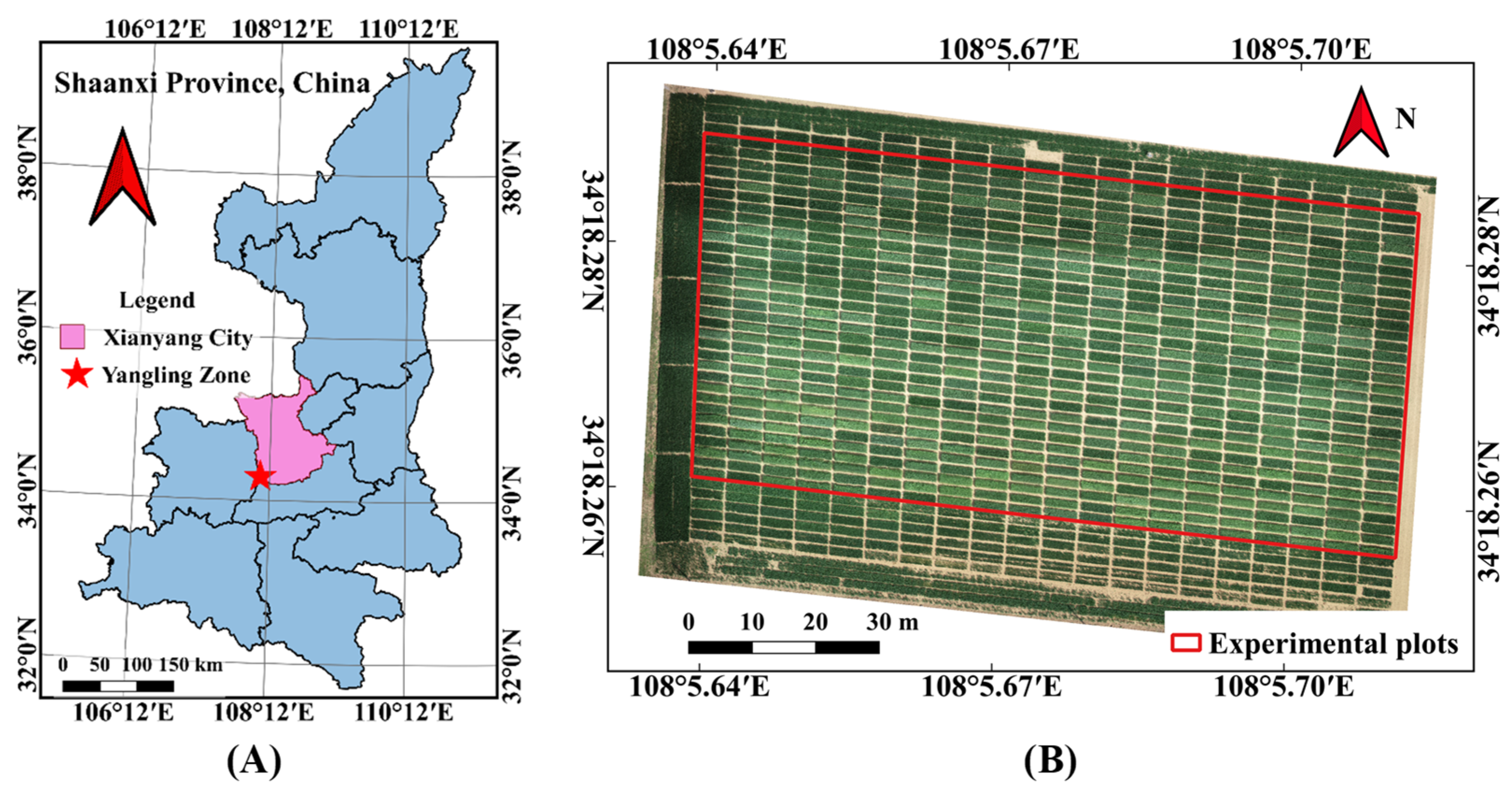
This study was carried out on Cao Xinzhuang experimental farm (34°18′15″ N, 108°5′40.77″ E) in Yangling, Shaanxi, China (Figure 1) from April to June 2021. The test area belongs to a warm temperate zone and is semi-humid and semi-arid region of east Asia. The average annual temperature and precipitation in this area is about 13.0 °C and 630 mm, respectively, and the rainfall in recent years is mainly concentrated from August to October. There were 565 wheat (Triticum aestivum L.)genotypes in this study, including the main domestic varieties, core germplasm, local farm varieties, backbone parents, representative varieties of different periods in China, and critical materials introduced from abroad. The experiment adopted a nonreplicated augmented design with five replicated check varieties (‘Zhoumai18’, ‘Jimai22’, ‘Bainong207’, ‘Xinong511’, and ‘Yanzhan4110’) and plots of 6 m2 (1.2 m wide × 5 m long) with six rows spaced 0.20 m apart. A total of 640 sample plots were planted in 18 October 2020 with a planting density of 270 plants/m2. The organic matter, pH value, -N, -N, available phosphorus, and available potassium of the soil (0–40 cm) in this experimental field were 13.66–15.25 g/kg, 7.89–8.10, 0.38–0.51 mg/kg, 27.70–35.60 mg/kg, 9.96–14.41 mg/kg, and 137.72–153.03 mg/kg, respectively. Wheat samples were protected from weeds, pests, and diseases during growth. For follow-up analysis, we selected 450 samples (including 406 genotypes) with a slight phenological difference and without lodging in a late growth period.
2.2. Rainfall and Air Temperature Records
It was known from the National General Weather Station in Yangling, China that there were three rainfalls during the test period, specifically about 41 mm from April 23 to 25, 15 mm from May 2 to 3, and 32 mm from May 14 to 15. A field weather station recorded the daily air maximum, minimum and average temperature during the test period in this experimental field (Figure 2).
2.3. Data Acquisition
Two high-throughput platforms were used to collect data in this study. One was DJI Phantom 4 Real-Time Kinematic (RTK) (DJI Technology, Shenzhen, China) integrated with a low-cost digital camera (COMOS sensor) to record RGB images (spatial resolution: 5472 × 3648 pixels) containing geographic location information. Another was Matrice 200 V2 UAV (DJI Technology, Shenzhen, China) equipped with a Micasense Altum (AL08) multispectral camera (Micasense, Seattle, WA, USA). The multispectral platform could record five spectral band images (spatial resolution: 2064 × 1544 pixels) with geographic location information at the same time and these bands and their respective central wavelength (band width) were specifically Blue (B), 475(32) nm; Green (G), 560(27) nm; Red (R), 668(16) nm; Red Edge (RE), 717(12) nm; and Near Infrared (NIR), 840(57) nm. In addition, the downwelling light sensor (DLS) was used to correct for ambient light and solar angle changes during flight, and the calibrated reflectance panel (CRP) was used to calibrate the bands’ reflectance in a multispectral platform, and these were not available in the RGB platform. From wheat heading to maturity, multi temporal data was acquired at the sunny midday with light cloud, low wind and appropriate sun angles to ensure the ambient light was relatively consistent and there was no UAV shadow in each acquired image during the flight. We investigated and recorded the development or phenology stages of the wheat population with the Feekes Scale [2] method (more details were given in Table 1).
2.4. Data Processing and Indices Extraction
Firstly, the original single RGB and multispectral images of wheat canopy with continuous geographical position obtained by UAV were mosaicked by Pix4D mapper 4.5.6 software (https://www.pix4d.com/, accessed date: 1 October 2021) to generate the orthophoto maps of each channel in the RGB space and five spectral bands in multispectral imaging. For multispectral images, irradiance compensation and radiometric and reflectance calibration were performed with the irradiance data recorded by DLS and reflectivity calibration coefficients in CRP during image mosaic pre-processing. Then, the geographic correction of orthophoto maps was executed based on ground control points (GCPs) through Quantum GIS (QGIS) 3.10.10 software (https://www.qgis.org/en/site/, accessed date: 1 October 2021) to calibrate the geographical position deviation of different stages of images. We made the shapefile of each plot and cropped the plots based on their respective shapefile in QGIS and the Green Leaf Index (GLI) map in RGB, and the normalized difference vegetation index (NDVI) map in the MSI of the wheat heading stage were segmented using the threshold method (the threshold was set to 0.1 in GLI and 0.5 in NDVI) to generate mask images for removing the background. Finally, diversified indices constructed from visible or near-infrared bands in RGB and MSI were calculated in MATLAB2020a software (https://ww2.mathworks.cn/, accessed date: 6 October 2021). The definition and formulas of the indices applied in this study were shown in Table 2, and indices were divided into the following types: 10 visible color indices (CIs) of RGB (RGB_CIs), 10 visible CIs of MSI (MSI_CIs), and 11 visible and near-infrared (Vis/Nir) spectral indices(SIs) of MSI (MSI_SIs).
2.5. Data Analysis Methods
Firstly, four types of indices, namely RGB_CIs, MSI_CIs, MSI_SIs and MSI_CIs + SIs (MSI_CIs + MSI_SIs) were respectively used to classify four key stay green stages by machine learning classifiers to determine RGB and MSI feasibility preliminarily in SG phenotyping. The stages were the anthesis stage (S1), watery ripe stage (S2), mealy ripe stage (S3), and kernel hard stage (S4), and their data was correspondingly obtained on 30 April, 12 May, 24 May, and 1 June. Here, Support Vector Machine (SVM), Quadratic Discriminant Analysis (QDA), K-Nearest Neighbor (KNN), and Ensemble Learning (EL) classifiers were taken for stage classification, and these supervised algorithms had been widely used in state detection and featured analysis in plant science [50,51,52,53]. We used classifier classification accuracy and confusion matrix to assess the validity of input indices and tools’ phenotyping potential.
Secondly, all indices’ change trends during SG decay were analyzed with high temporal resolution data for selecting the indices with a monotonous variation on the whole and obvious relative change ratios in the heading stage and maturity stage. To quantitatively compare the SG between genotypes, the wheat sample’s relative stay green rates (SGR) were proposed and calculated based on the relationship between senescense and stay green with the time series of selected indices. Here, index SGR was abbreviated as SG_Index; for example, NDRE SGR was abbreviated as SG_NDRE, while the SGR of GLI in RGB and MSI was abbreviated as SG_ GLI_ RGB and SG_GLI_MSI. The state of wheat at the heading stage was used as the maximum SGR reference (100%), and the index at this stage was labeled as Index_S0, and the index of the i stage (such as anthesis stage, water ripe stage, and mealy ripe stage) was labeled as Index_Si. Wheat senescence rate at i stage (SenR_Index_Si) was calculated according to Equation (1) and stay green rate at i stage (SG_Index_Si) was calculated according to Equation (2).
Thirdly, we substituted the time series data of each selected index into the above two equations to calculate its temporal SGR. Moreover, the dynamics of selected indices SGR from flowering to maturity stages were analyzed and their correlations with samples’ yield were evaluated and compared using Multiple Linear Regression (MLR), and linear Support Vector Regression (SVR). To explore the index SGR feasibility as an alternative to visual assessment, the dynamics of some indices’ SGR with different yield correlations were compared in tracking three stay green grade samples identified by manual visual scoring at late growth stages.
3. Results
3.1. Stay Green Stages Classification Results
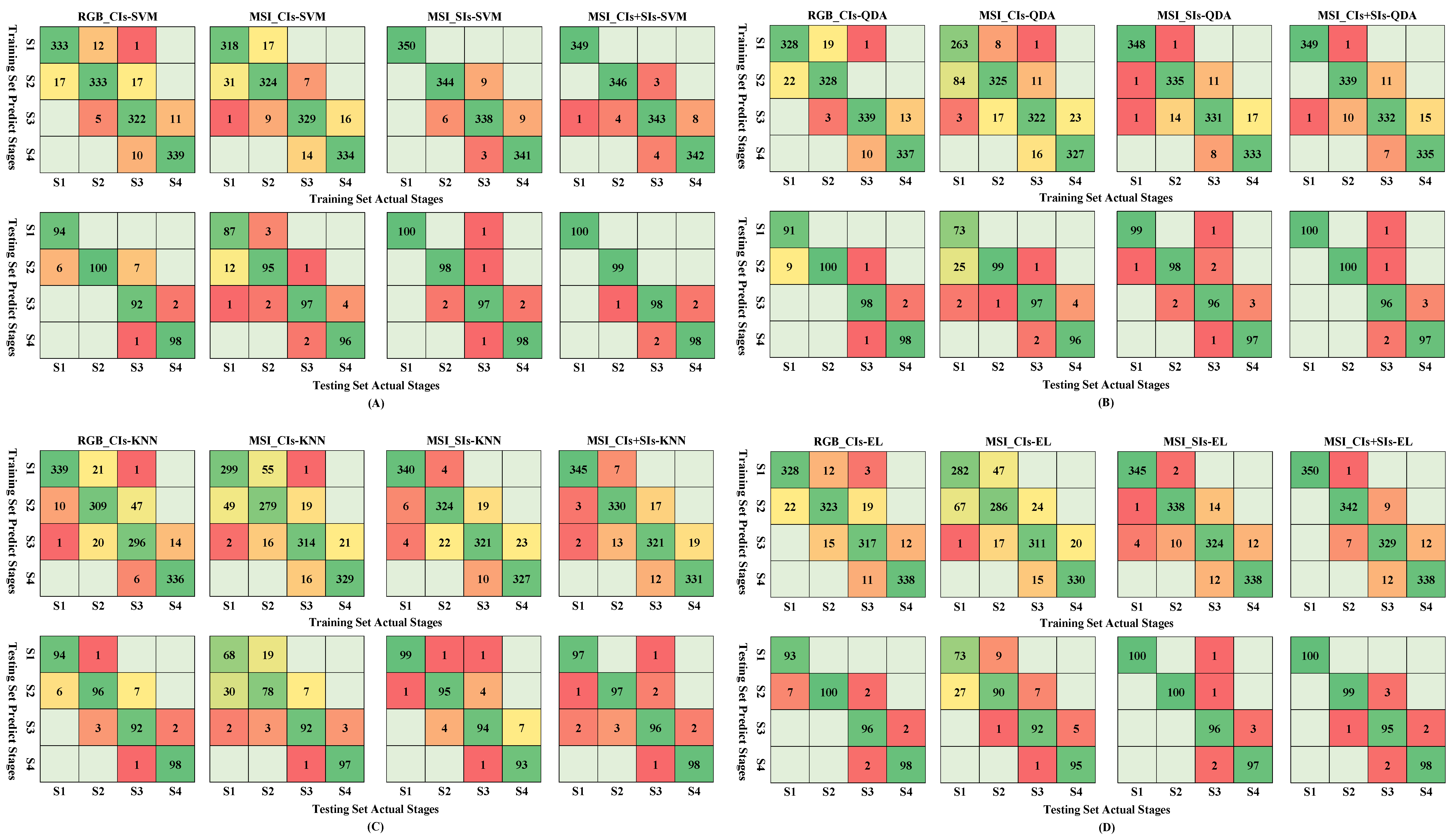
The 450 samples in the wheat population at each stage were divided into the training set (350 samples) and test set (100 samples) by the Kennard–Stone [54] algorithm, and all training samples (1400 samples) and test samples (400 samples) were used for classifier training and testing, respectively. SVM (cubic polynomial as kernel function), QDA, KNN (10 neighbors and Euclidean distance measure), and EL (Adaboost method with 1000 discriminant learners) models with 10-fold cross-validation were built by scale-adjusted indices of each type. All indices obtained acceptable results, and their best average classification accuracy in training and test sets attained 93.20–98.60% and 93.80–98.80%, respectively (Table 3). They indicated that RGB and MSI could detect different stay green stages of the wheat population to a certain extent. Specifically, RGB_CIs obtained better results than MSI_CIs, but not than MSI_SIs, and MSI_CIs + SIs contained nearly twice as many indices as MSI_Vis/Nir_11indices, but its results were only slightly improved. Classifier confusion matrices of S1, S2, S3, and S4 presented the visualization results in more detail and showed the same comparison results as above (Figure 3), and the misclassified samples were mainly concentrated in adjacent stages.
3.2. Indices Dynamics Analysis Results
The time series curves of image-based indices were indirect tools to describe crop growth, and we screened indices with such monotonous variations as SG unidirectional decay during grain filling. Moreover, index correlations and relative average variation ratios in heading and maturity stages were also used to simplify the number of analyzed indices.
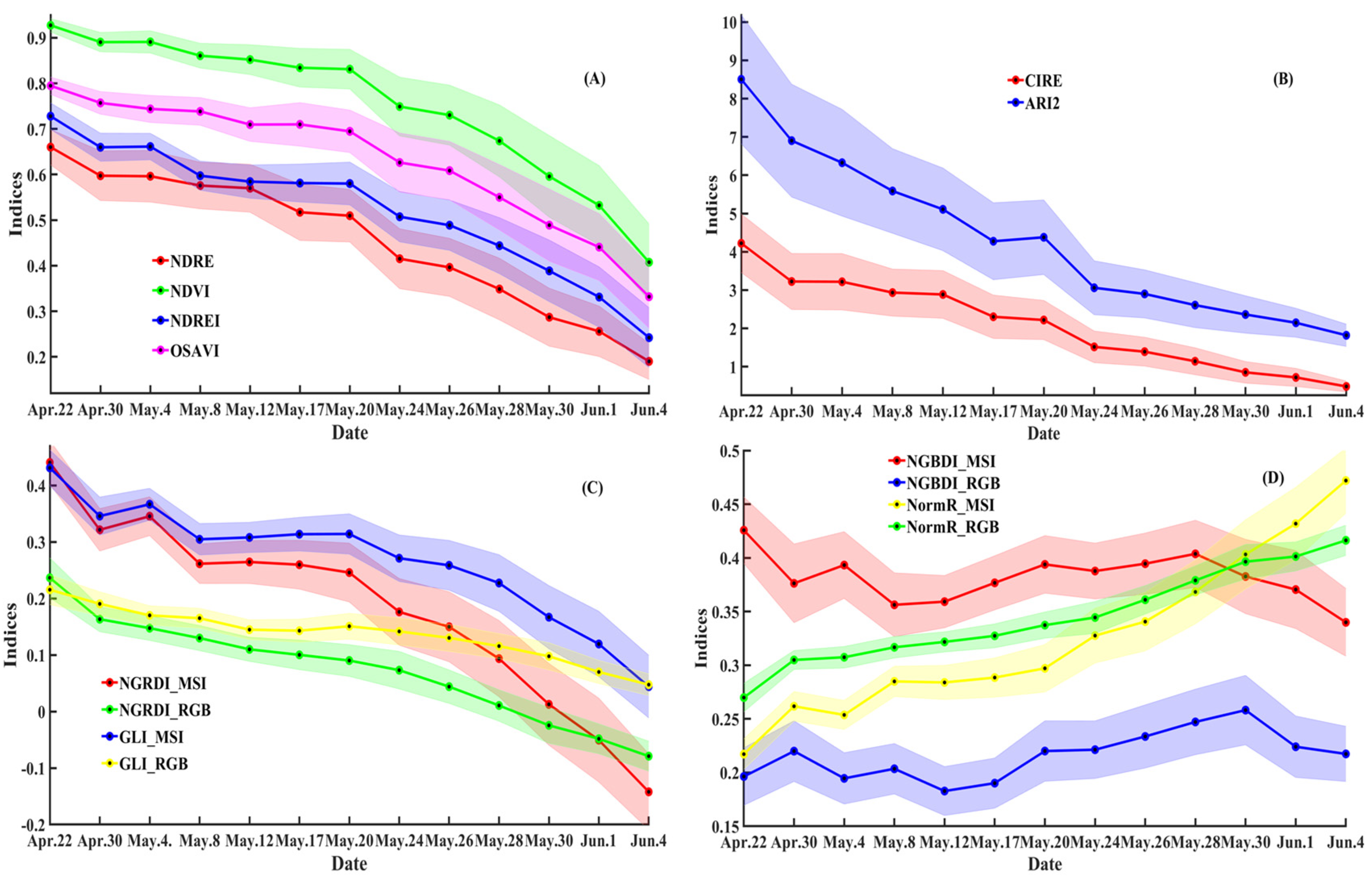
Index trends were recorded (Table 4 and Table 5), and their dynamics generally showed three types from heading to maturity. The first type was a monotonous decline with two modes. One mode was a slow decline in the early and middle stage, the fast decline in late-stage and indices of this mode included NDRE, NDVI, NDREI, OSAVI (Figure 4A), GNDVI, BNDVI, GNDREI, and BNDREI in MSI and GLI, NGRDI (Figure 4C), NormG and GR in both sensors. The other mode was a fast decline in the early and middle stage, slow decline in late-stage, and CIRE, ARI2 (Figure 4B), and ARI1 belonged to this mode. The second type was a monotonic rise and rose slowly in the early and middle stage and fast in the late stage, and NromR (Figure 4D) and ExR in both sensors were this type. The third type was nonmonotonic as NGBDI (Figure 4D) and NormB in two sensors and the ExG in MSI.
In color indices, decline-type indices (NGRDI, GLI, GR, VARI) had high correlations with rising-type indices (NormR and ExR) and low correlations with fluctuating-type indices (NormB and NGBDI) (Figure 5A,B). In MSI_SIs, there were high correlations (0.95–0.99) between NDRE, NDVI, GNDVI, BNDVI, NDREI, and OSAVI and the correlations (0.92–0.98) between CIRE, ARI1 and ARI2 were also high, but the correlations (0.38–0.79) between GNDREI and BNDREI and other indices were low (Figure 5C). In RGB monotonic indices, the relative average variation ratios in heading and maturity of NormR, NGRDI, GLI, GR, VARI, ExG, and ExR (47.96–463.38%) were greater than NormG and NormB (18.76% and 21.84%). In MSI monotonic indices, the relative variation ratios of NDVI, OSAVI, ARI1, NDREI, NDRE, GR, ARI2, CIRE, GLI, NormR, VARI, NGRDI, and ExR (55.99–615.19%) were also greater than BNDREI, GNREI, BNDVI, NormB, NormG, and GNDVI (13.09–38.13%). The above results selected NDRE, NDVI, NDREI, CIRE, ARI2 in MSI and NormR, NGRDI, GLI, GR, VARI in RGB and MSI.
3.3. Stay Green Rates Dynamics Results
It is crucial in high-throughput phenotyping for wheat stay green to construct interpretable secondary phenotypes that cloud, distinguish, and quantify stay green based on image indices curves. We used the time series of selected indices to calculate wheat samples’ relative stay green rates (SGR) and summarize their overall change trends (mean/sd) and they generally declined with populations’ SG decay and showed various decline characteristics in different stages (Table 6). SG_NDRE, SG_CIRE, SG_ARI2, SG_NGRDI, and SG_VARI saturation effects were smaller than other index rates, such as SG_NDVI, SG_NDREI, and SG_NormR in the initial grain filling stage. We further verify these indices’ SGR validity by counting the numerical interval of about the top 90% samples in Pareto distribution histograms at the anthesis stage (S1), watery ripe stage (S2), mealy ripe stage (S3), and kernel hard stage (S4) (Table 7). It could be seen that these indices’ SGR in most samples had interval separations in different stages, especially in the S1, S3, and S4 stages. Moreover, SG_NDREI, SG_CIRE, SG_ARI2, SG_NGRDI, SG_GLI interval overlap were less than SG_NDRE, SG_NDVI, SG_NormR, etc between S1 and S2. These results suggested that SGR indices may be alternative tools to reveal the dynamic changes of stay green in wheat populations.
3.4. Yield Regression Results
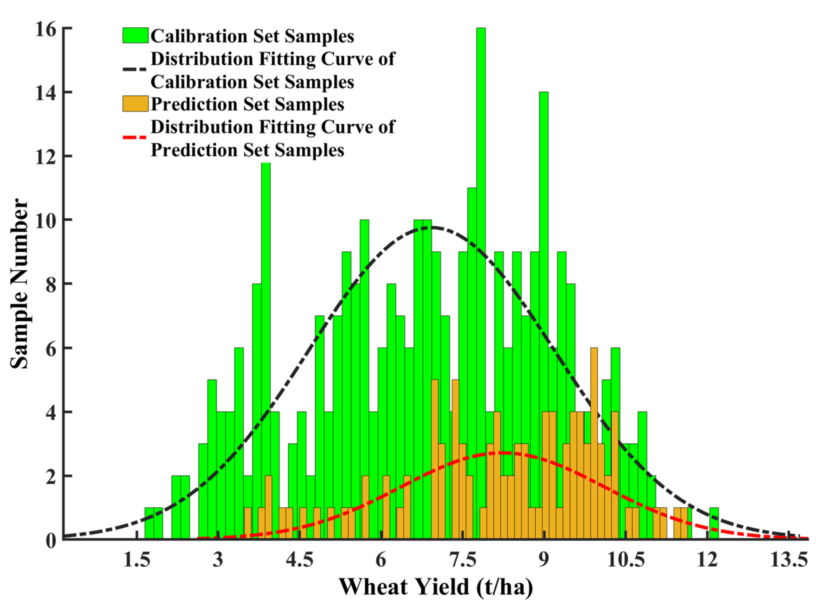
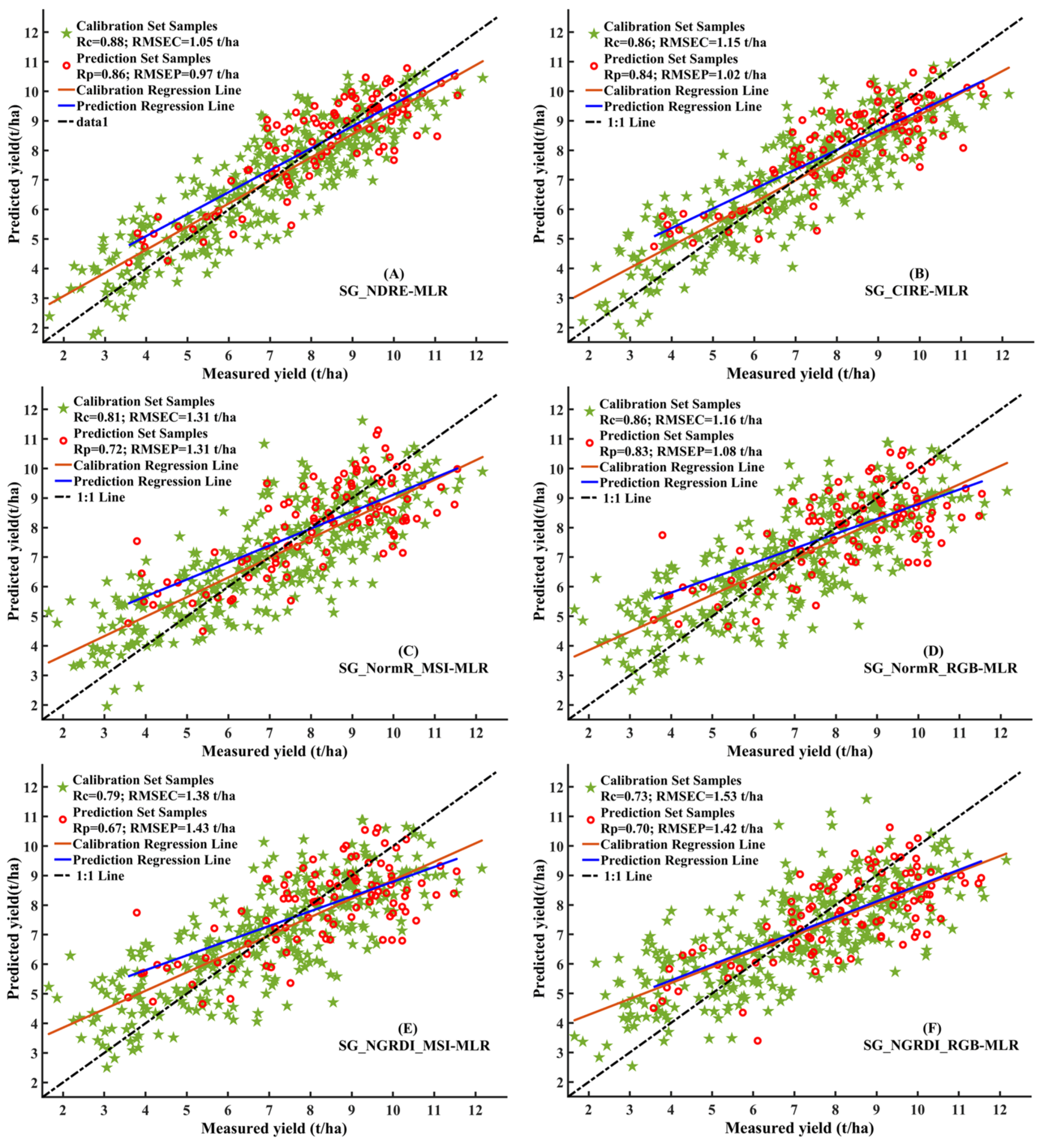
We used MLR and linear SVR to compare indices’ temporal SGR correlations with sample yields, considering that the dynamics of wheat stay green were mainly concentrated in the yield formation stage. The 435 samples (eliminating some yield outliers from 450 samples) were divided into a calibration set (335 samples) and prediction set (100 samples) using sample set partitioning based on a Joint X-Y Distance [54] algorithm for regression calibration and prediction. All samples’ yield mean and standard deviation were 7.23 t/ha and 2.24 t/ha, respectively, and the yield distribution range of the prediction set (3.45–11.70 t/ha) was within the range of the calibration set (1.65–12.15 t/ha) (Figure 6). For yield regression, MLR models were generally better than linear SVR models with higher correlation coefficients of the calibration and prediction set (Rc and Rp) and lower root mean square error of the calibration and prediction set (RMSEC and RMSEP) (Table 8). Among MLR results, SG_NDRE, SG_CIRE, SG_NDVI and SG_NormR_RGB obtained a high correlation (Rc >0.85 and Rp > 0.8) and low error (RMSEC < 1.17 t/ha and RMSEP < 1.12 t/ha) and SG_NGRDI and SG_VARI in MSI and RGB had low correlation (Rc < 0.80 and Rp < 0.72) and high error (RMSEC > 1.38 t/ha and RMSEP > 1.39 t/ha). Other indices’ SGRs, such as SG_NormR and SG_GLI in MSI, obtained medium correlations with sample yield. In MLR models, the measured and predicted yields were closer to each other in scatter plots of high correlation (SG_NDRE, SG_CIRE and SG_NormR_RGB) than medium (SG_NormR_MSI) and low (SG_NGRDI_MSI and SG_NGRDI_RGB) correlations (Figure 7).
3.5. SGR Dynamics in Visual Stay Green Grades
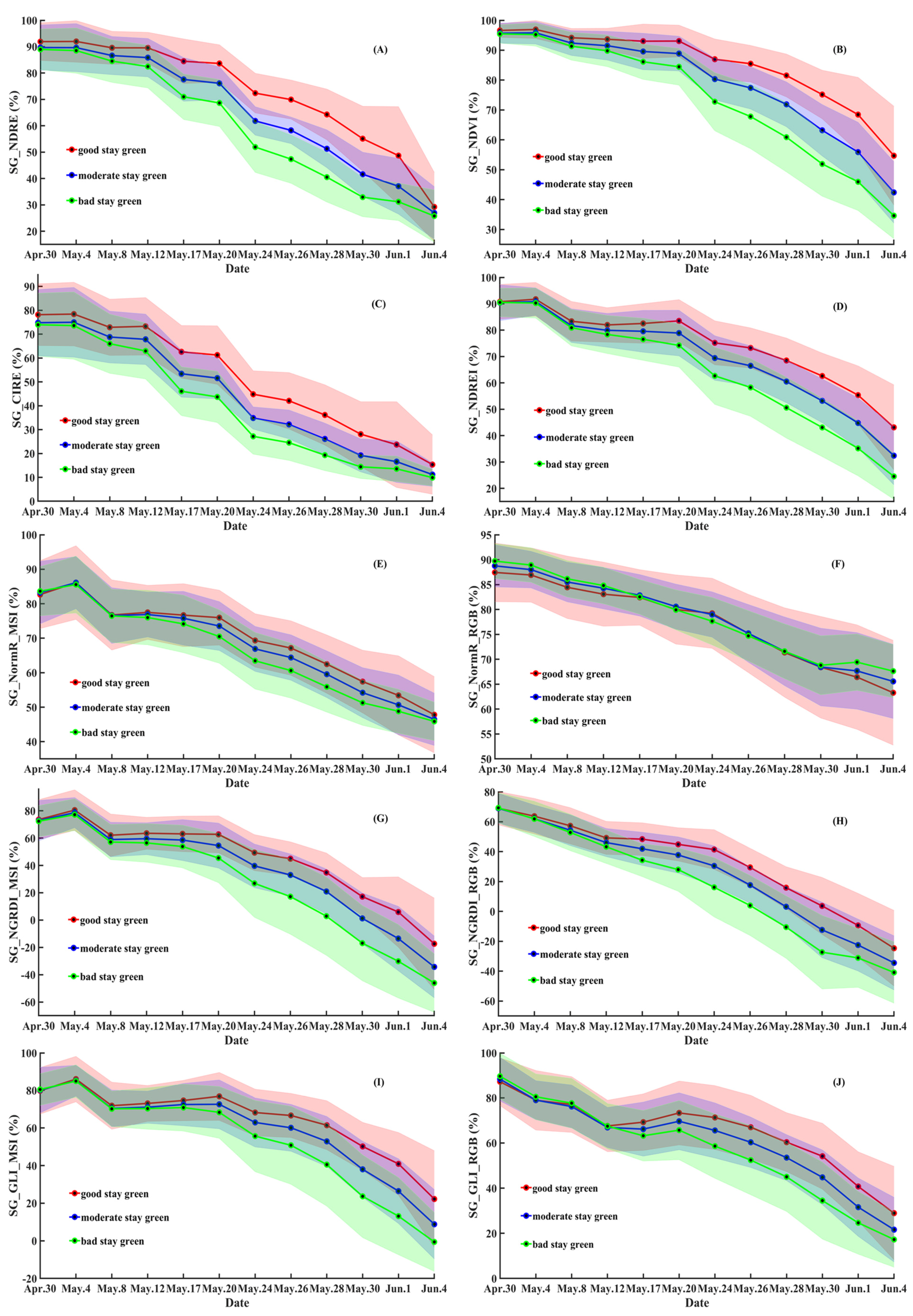
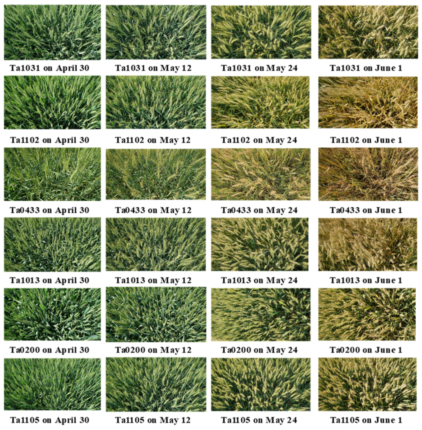
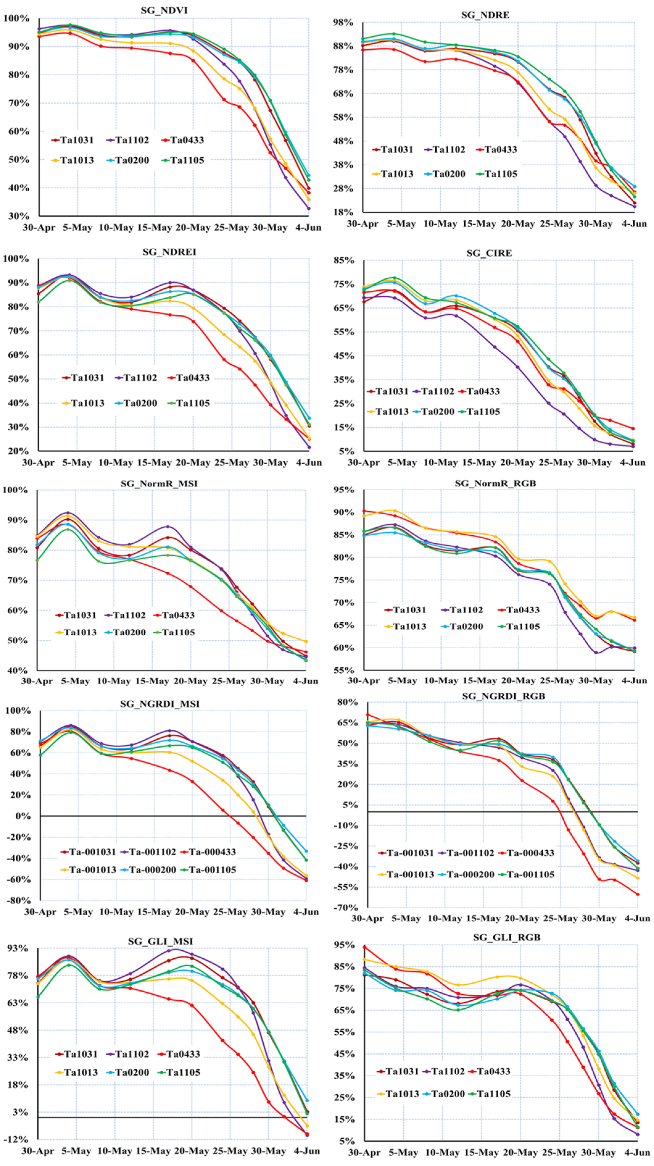
According to the guidances of [3] and [37], we visually identified the stay green grade of the samples by visually scoring whole plant senescence and the portion of green leaf area in the flag leaf at the middle and later grain filling stages. Moreover, three stay green grades of genotypes, namely good stay green, moderate stay green, and bad stay green, were preliminarily identified. We selected 90 samples of each grade with obvious visual grade differences and analyzed their dynamics (mean and 95% confidence interval) of some indices’ SGRs with high, medium and low yield correlations in three grade samples (Figure 8). There were good distinctions for three grade samples in SG_NDRE, SG_NDVI and SG_CIRE dynamics at the early, middle and late stage. Additionally, there were also grade samples distinctions in the dynamics of SG_NDREI, SG_NormR_MSI, SG_NGRDI_MSI, SG_NGRDI_RGB, SG_GLI_MSI, and SG_GLI_RGB at the middle and late stage. However, there was no good distinction for three grade samples all the time in the SG_NormR_RGB dynamic. Moreover, we compared the indices’ SGR curves in Figure 8 in six samples (labeled Ta1031, Ta1102, Ta0433, Ta1013, Ta0200, and Ta1105) selected from three grade samples (Figure 9). Similarly, SG_NDRE and SG_NDVI could potentially distinguish the late senescent (Ta1031, Ta0200, and Ta1105), middle senescent (Ta1102, Ta1013), and the early senescent (Ta0433) samples at the early, middle or late stage, and SG_NDREI, SG_CIRE and SG_NormR_MSI, SG_NGRDI and SG_GLI of MSI and RGB could distinguish different senescent types at the late stage (Figure 10), while SG_NormR_RGB did not have differentiation potential. Moreover, SG_NDREI and SG_NormR_MSI, SG_NGRDI and SG_GLI were more susceptible to rainfall and temperature changes (2–3 May and 14–15) than SG_NDRE, and SG_NDVI in MSI. This indicated that indices’ SGRs derived from RGB and MSI could replace manual visual evaluation to a certain extent.
4. Discussion
This study compared the availability of UAV-based RGB and MSI for stay green phenotyping in the wheat population and attempted to develop high-throughput phenotyping methods for wheat stay green with two tools to improve the phenotyping efficiency and accuracy in the field breeding.
4.1. Stay Green Stages Detection
It is a premise for wheat stay green phenotyping to distinguish different stay green stages effectively. The color index classification performances in RGB were better than in MSI in this study, which might mean that RGB provided more color information than MSI. RGB camera used a single camera lens with prismatic decomposition to record R, G, and B channel images. In contrast, multispectral cameras used multi lens with multiple narrowband optical bandpass filters to record specific band images and this made the spectral range of R, G, and B channels in a RGB camera wider than in multispectral camera, as mentioned in [24]. The color indices in MSI could reveal more detailed color information, and they were also more vulnerable to rainfall than RGB color indices. Although RGB color indices in this study obtained an acceptable classification result, it could not be ignored that the quality of RGB data is easily affected by illumination changes (changes in illumination strength or sudden clouds) in the field [55,56,57,58]. Therefore, it needs to develop more targeted frameworks to calibrate these uncontrollable factors to obtain stable and reliable data for a low-cost RGB imaging platform. MSI_SIs and MSI_Cis + SIs obtained similar and better results than color indices, and this indicated the red edge and near-infrared reflection spectrum have greater potential in revealing more details (like micro phenotype response). It is understandable that the vegetation visible reflection spectrum mainly reflects crops’ external color traits and rarely contains internal biochemical information. Red edge and near-infrared reflection spectrum are mainly related to plants’ internal cell structures (nitrogen, protein, chlorophyll, etc.) [37,59]. In most cases, the change in plant external color or visible traits would lag behind the internal invisible biochemical phenotype response. So, the multispectral imaging technique has more application potential than RGB imaging in revealing wheat senescence or stay green states.
4.2. Indices Dynamic Analysis
Wheat senescence is a programmed death process, and SG is also a complex dynamic trait, which is difficult to determine by an isolated developmental state, especially in population samples with diversified genotypes. Temporal image indices have been used to describe and reveal crop growth dynamics in many studies and there were various dynamics for image indices in this study. Wheat senescence is mainly due to the competition for assimilates of sinks from sources and it generally includes slow and rapid senescent periods. In the slow senescent period, canopy greenness or vigor decay were slow as there was not much competition. The grains were mainly kernel length in establishment in the early stage (rapid increase in grain size with little dry matter accumulation). In the rapid senescent period, canopy greenness or vigor decay were fast as the competition became fierce in the middle and late stage (milky ripe stage) due to grains requiring many photosynthates to accumulate solid content until the kernels achieve maximum dry weight and physical maturity [9,11]. For canopy greenness, vigor or green leaf area, they showed a slow decline in the early stage and rapid decline in the middle and late stages during wheat senescence [60]. The dynamics of NDRE, NDVI, NDREI, NGRDI, GLI, NormR, and VARI in RGB or MSI traced the trend of slow first and then fast in the same or opposite ways in this study and these indices could be used as the integrative measurements of the overall amount and quality of photosynthetic material in plants or the combined effects of leaf chlorophyll content, canopy leaf area or architecture. Chlorophyll is a common indicator of stay green and its degradation marks the start of senescence and it is the leaves in the middle and lower part of wheat rather than the flag leaves that turn on senescence first. The Red Edge Chlorophyll Index (CIRE) was designed with NIR and red edge (RE) bands to estimate leaf chlorophyll content [45] and the red edge (690–740 nm) was caused by the transition from chlorophyll absorption and NIR leaf scattering, and NIR had greater penetration depth in the plant canopy. Indices combined by RE and NIR bands are more sensitive to smaller plant changes and responses in deeper vertical canopy directions. ARI1 and ARI2 are used to reflect the changes in stress-related pigments, which are present in higher concentrations in weakened plants (mainly anthocyanins, the pigments abundant in newly forming and undergoing senescence leaves). Weakening crops contain higher concentrations of anthocyanins, and this index is one measure of stressed crops [46]. So, the multispectral sensor could provide more monotonically varying indices, and the phenotypes associated with these indices are richer than RGB color indices. The time series curves of color and spectral indices derived from RGB and multispectral images could describe the development of wheat senescence from a macro or micro phenotype.
4.3. Indices SGR Dynamic Analysis
The relative stay green rates (SGR) were proposed and derived from index curves as secondary phenotypes to quantify the stay green differences in diversified genotypes. From the results of yield regression, indices’ temporal SGRs showed potential to predict yield and might provide a new perspective for yield prediction. In recent years, some studies directly used temporal color or spectral indices (NDRE, NDVI, NGRDI, GLI, VARI, ExG, etc.) to establish crop yield prediction models and showed indices’ validity in yield evaluation and revealing the contribution of different stages to yield [27,29,36]. However, there would be temporal and spatial differences in indices obtained in different seasons or environments, and that could affect yield model robustness. Here, SGR was a relative secondary trait derived from color or spectral index time series curves, which took the sample itself as the reference, so this might provide a calibration reference for image-based indices in multiple environments.
At the anthesis stage, the SGR of color indices (especially NGRDI, and VARI), ARI2 and CIRE were lower, and this might imply that these indices were more sensitive to short-term heat stress (>30 °C, shown in Figure 2) between heading and flowering stages than other indices such as NDRE, NDVI and NDREI. Moreover, these indices SGR showed a similar difference in short-term heat stress from May 4 to May 8. The short-term heat stress could induce cell dehydration, leaf water loss or wilt, and color change, and damage leaves’ chloroplast structure and alter canopy photosynthetic pigments (chlorophyll and carotenoids) and stress-related pigments concentrations [61,62]. So, the SGR of these sensitive indices could be used to analyze the response of populations to heat stress, which is a common environmental stress at the wheat growth anaphase.
The time series of index SGRs could effectively discriminate SG changes from the population level, but they were different in tracking the dynamics of samples with different visual green grades. SG_NDRE, SG_CIRE, and SG_NDVI obtained good results in tracking visually observed stay green grades in diversified genotypes, and they could be alternative tools for visual assessment, which showed that the red edge and near infrared reflection spectrum may be more effective once again. For color indices, SG_GLI and SG_NGRDI in RGB and MSI and SG_NormR_MSI could track visual stay green grades in later grain filling stages but could not capture the phenotype response of visual grade samples at the early stage, and this indicated that the canopy color response of different stay green grade samples was lagging behind their biochemical phenotype response. Moreover, the color phenotype was easily affected by external environmental factors such as rainfall. SG_NormR_RGB failed to track visual grade samples, in which the spectral ranges might cause overlap of the R, G, and B channels in the RGB camera, as mentioned in [24]. In addition, the potential of these secondary phenotypes in assisting genome-wide analysis could be considered, and we hoped to verify their differences and effectiveness in the mapping of SG-associated genes by genome-wide association analysis in the next work.
5. Conclusions
The efficiency of SG phenotyping in wheat field breeding can be significantly increased using appropriate HTP platforms and reliable analysis methods. The study initially demonstrated the potential of the indices derived from RGB and 5-band multispectral images in the SG phenotyping of diversified wheat genotypes. The temporal indices could track the phenology of wheat in the late growth stage with different variation forms, and indices containing the red edge or near-infrared band could reveal more microscopic details than indices containing only visible bands. Based on the dynamic curves of monotonic indices, the proposed SGR can serve as interpretable secondary phenotypes to quantitatively compare the SG differences in wheat genotypes. The SGR of MSI indices (NDRE, CIRE and NDVI) showed higher correlations with samples’ yield and more timely potential to distinguish different SG grades samples than that of color indices in RGB and MSI. The SGR of the color indices (NGRDI, GLI) in MSI were more specific in revealing changes in color phenotypes than in RGB. All in all, the performance of the multispectral imaging platform in this study is better than the low-cost RGB imaging platform in SG phenotyping of diversified wheat germplasm.
Author Contributions
Conceptualization, X.C. and Y.L.; methodology, X.C., D.H. and Y.L.; software, X.C., B.S. and Y.L.; formal analysis, X.C. and Y.L.; investigation, X.C., R.Y. and Y.L.; writing—original draft preparation, X.C.; writing—review and editing, D.H. and B.S. All authors have read and agreed to the published version of the manuscript.
Funding
This study was supported financially by International Cooperation and Exchange of the National Natural Science Foundation of China (Grant no. 31961143019).
Data Availability Statement
Data will be available from the author upon reasonable request.
Acknowledgments
We acknowledge the support provided by the members of Wheat Disease Resistance Genetics and Molecular Breeding Program, Northwest A&F University.
Conflicts of Interest
The authors declare no conflict of interest.
References
- Dowla, M.A.N.N.; Edwards, I.; O’Hara, G.; Islam, S.; Ma, W. Developing Wheat for improved yield and adaptation under a changing climate: Optimization of a few key genes. Engineering 2018, 4, 514–522. [Google Scholar] [CrossRef]
- Hyles, J.; Bloomfield, M.T.; Hunt, J.R.; Trethowan, R.M.; Trevaskis, B. Phenology and related traits for wheat adaptation. Heredity 2020, 125, 417–430. [Google Scholar] [CrossRef] [PubMed]
- Chapman, E.A.; Orford, S.; Lage, J.; Griffiths, S. Capturing and selecting senescence variation in wheat. Front. Plant Sci. 2021, 12, 638738. [Google Scholar] [CrossRef]
- Joshi, S.; Choukimath, A.; Isenegger, D.; Panozzo, J.; Spangenberg, G.; Kant, S. Improved wheat growth and yield by delayed leaf senescence using developmentally regulated expression of a cytokinin biosynthesis gene. Front. Plant Sci. 2019, 10, 1285. [Google Scholar] [CrossRef] [Green Version]
- Chapman, E.A.; Orford, S.; Lage, J.; Griffiths, S. Delaying or delivering: Identification of novel NAM-1 alleles which delay senescence to extend wheat grain fill duration. J. Exp. Bot. 2021, 72, 7710–7728. [Google Scholar] [CrossRef] [PubMed]
- Christopher, J.T.; Christopher, M.J.; Borrell, A.K.; Fletcher, S.; Chenu, K. Stay-green traits to improve wheat adaptation in well-watered and water-limited environments. J. Exp. Bot. 2016, 67, 5159–5172. [Google Scholar] [CrossRef] [PubMed] [Green Version]
- Kamal, N.M.; Gorafi, Y.S.A.; Abdelrahman, M.; Abdellatef, E.; Tsujimoto, H. Stay-Green Trait: A Prospective Approach for Yield Potential, and Drought and Heat Stress Adaptation in Globally Important Cereals. Int. J. Mol. Sci. 2019, 20, 5837. [Google Scholar] [CrossRef] [Green Version]
- Munaiz, E.D.; Martinez, S.; Kumar, A.; Caicedo, M.; Ordas, B. The Senescence (Stay-Green)-An Important Trait to Exploit Crop Residuals for Bioenergy. Energies 2020, 13, 790. [Google Scholar] [CrossRef] [Green Version]
- Lv, X.; Zhang, Y.; Zhang, Y.; Fan, S.; Kong, L. Source-sink modifications affect leaf senescence and grain mass in wheat as revealed by proteomic analysis. BMC Plant Biol. 2020, 20, 257. [Google Scholar] [CrossRef]
- Sade, N.; Rubio-Wilhelmi, M.D.M.; Umnajkitikorn, K.; Blumwald, E. Stress-induced senescence and plant tolerance to abiotic stress. J. Exp. Bot. 2018, 69, 845–853. [Google Scholar] [CrossRef]
- Sultana, N.; Islam, S.; Juhasz, A.; Ma, W. Wheat leaf senescence and its regulatory gene network. Crop J. 2021, 9, 703–717. [Google Scholar] [CrossRef]
- Scossa, F.; Alseekh, S.; Fernie, A.R. Integrating multi-omics data for crop improvement. J. Plant Physiol. 2021, 257, 153352. [Google Scholar] [CrossRef] [PubMed]
- Cortes, L.T.; Zhang, Z.; Yu, J. Status and prospects of genome-wide association studies in plants. Plant Genome. 2021, 14, e20077. [Google Scholar] [CrossRef]
- Song, P.; Wang, J.; Guo, X.; Yang, W.; Zhao, C. High-throughput phenotyping: Breaking through the bottleneck in future crop breeding. Crop J. 2021, 9, 633–645. [Google Scholar] [CrossRef]
- Moreira, F.F.; Oliveira, H.R.; Volenec, J.J.; Rainey, K.M.; Brito, L.F. Integrating high-throughput phenotyping and statistical genomic methods to genetically improve longitudinal traits in crops. Front. Plant Sci. 2020, 11, 681. [Google Scholar] [CrossRef]
- Cao, X.; Yu, K.; Zhao, Y.; Zhang, H. Current status of high-throughput plant phenotyping for abiotic stress by imaging spectroscopy: A review. Spectrosc. Spect. Anal. 2020, 40, 3365–3372. [Google Scholar] [CrossRef]
- Guo, W.; Carroll, M.E.; Singh, A.; Swetnam, T.L.; Merchant, N.; Sarkar, S.; Singh, A.K.; Ganapathysubramanian, B. UAS-based plant phenotyping for research and breeding applications. Plant Phenomics. 2021, 2021, 9840192. [Google Scholar] [CrossRef] [PubMed]
- Yang, G.; Liu, J.; Zhao, C.; Li, Z.; Huang, Y.; Yu, H.; Xu, B.; Yang, X.; Zhu, D.; Zhang, X.; et al. Unmanned aerial vehicle remote sensing for field-based crop phenotyping: Current status and perspectives. Front. Plant Sci. 2017, 8, 1111. [Google Scholar] [CrossRef]
- Feng, L.; Chen, S.; Zhang, C.; Zhang, Y.; He, Y. A comprehensive review on recent applications of unmanned aerial vehicle remote sensing with various sensors for high-throughput plant phenotyping. Comput. Electron. Agric. 2021, 182, 106033. [Google Scholar] [CrossRef]
- Clemente, A.A.; Maciel, G.M.; Silva Siquieroli, A.C.; de Araujo Gallis, R.B.; Pereira, L.M.; Duarte, J.G. High-throughput phenotyping to detect anthocyanins, chlorophylls, and carotenoids in red lettuce germplasm. Int. J. Appl. Earth Obs. 2021, 103, 102533. [Google Scholar] [CrossRef]
- Haghshenas, A.; Emam, Y. Image-based tracking of ripening in wheat cultivar mixtures: A quantifying approach parallel to the conventional phenology. Comput. Electron. Agric. 2019, 156, 318–333. [Google Scholar] [CrossRef]
- Zeng, L.; Wardlow, B.D.; Xiang, D.; Hu, S.; Li, D. A review of vegetation phenological metrics extraction using time-series, multispectral satellite data. Remote Sens. Environ. 2020, 237, 111511. [Google Scholar] [CrossRef]
- Zhou, M.; Ma, X.; Wang, K.; Cheng, T.; Tian, Y.; Wang, J.; Zhu, Y.; Hu, Y.; Niu, Q.; Gui, L.; et al. Detection of phenology using an improved shape model on time-series vegetation index in wheat. Comput. Electron. Agric. 2020, 173, 105398. [Google Scholar] [CrossRef]
- Brown, T.B.; Hultine, K.R.; Steltzer, H.; Denny, E.G.; Denslow, M.W.; Granados, J.; Henderson, S.; Moore, D.; Nagai, S.; SanClements, M.; et al. Using phenocams to monitor our changing Earth: Toward a global phenocam network. Front. Ecol. Environ. 2016, 14, 84–93. [Google Scholar] [CrossRef] [Green Version]
- Bukowiecki, J.; Rose, T.; Ehlers, R.; Kage, H. High-throughput prediction of whole season green area index in winter wheat with an airborne multispectral sensor. Front. Plant Sci. 2020, 10, 1798. [Google Scholar] [CrossRef] [PubMed]
- Tan, C.; Zhang, P.; Zhou, X.; Wang, Z.; Xu, Z.; Mao, W.; Li, W.; Huo, Z.; Guo, W.; Yun, F. Quantitative monitoring of leaf area index in wheat of different plant types by integrating NDVI and Beer-Lambert law. Sci. Rep. 2020, 10, 929. [Google Scholar] [CrossRef]
- Fei, S.; Hassan, M.A.; He, Z.; Chen, Z.; Shu, M.; Wang, J.; Li, C.; Xiao, Y. Assessment of ensemble learning to predict wheat grain yield based on uav-multispectral reflectance. Remote Sens. 2021, 13, 2338. [Google Scholar] [CrossRef]
- Kefauver, S.C.; Vicente, R.; Vergara-Diaz, O.; Fernandez-Gallego, J.A.; Kerfal, S.; Lopez, A.; Melichar, J.P.E.; Serret Molins, M.D.; Araus, J.L. Comparative UAV and field phenotyping to assess yield and nitrogen use efficiency in hybrid and conventional barle. Front. Plant Sci. 2017, 8, 1733. [Google Scholar] [CrossRef]
- Wan, L.; Cen, H.; Zhu, J.; Zhang, J.; Zhu, Y.; Sun, D.; Du, X.; Zhai, L.; Weng, H.; Li, Y.; et al. Grain yield prediction of rice using multi-temporal UAV-based RGB and multispectral images and model transfer—A case study of small farmlands in the South of China. Agric. Forest Meteorol. 2020, 291, 108096. [Google Scholar] [CrossRef]
- Munoz-Huerta, R.F.; Guevara-Gonzalez, R.G.; Contreras-Medina, L.M.; Torres-Pacheco, I.; Prado-Olivarez, J.; Ocampo-Velazquez, R.V. A review of methods for sensing the nitrogen status in plants: Advantages, disadvantages and recent advances. Sensors 2013, 13, 10823–10843. [Google Scholar] [CrossRef]
- Mishra, P.; Polder, G.; Vilfan, N. Close Range Spectral imaging for disease detection in plants using autonomous platforms: A review on recent studies. Curr. Robot. Rep. 2020, 1, 43–48. [Google Scholar] [CrossRef] [Green Version]
- Liedtke, J.D.; Hunt, C.H.; George-Jaeggli, B.; Laws, K.; Watson, J.; Potgieter, A.B.; Cruickshank, A.; Jordan, D.R. High-throughput phenotyping of dynamic canopy traits associated with stay-green in grain sorghum. Plant Phenomics. 2020, 2020, 4635153. [Google Scholar] [CrossRef]
- Rebetzke, G.J.; Jimenez-Berni, J.A.; Bovill, W.D.; Deery, D.M.; James, R.A. High-throughput phenotyping technologies allow accurate selection of stay-green. J. Exp. Bot. 2016, 67, 4919–4924. [Google Scholar] [CrossRef] [Green Version]
- Lopes, M.S.; Reynolds, M.P. Stay-green in spring wheat can be determined by spectral reflectance measurements (normalized difference vegetation index) independently from phenology. J. Exp. Bot. 2012, 63, 3789–3798. [Google Scholar] [CrossRef] [PubMed] [Green Version]
- Montazeaud, G.; Karatogma, H.; Ozturk, I.; Roumet, P.; Ecarnot, M.; Crossa, J.; Ozer, E.; Ozdemir, F.; Lopes, M.S. Predicting wheat maturity and stay-green parameters by modeling spectral reflectance measurements and their contribution to grain yield under rainfed conditions. Field Crop. Res. 2016, 196, 191–198. [Google Scholar] [CrossRef] [Green Version]
- Hassan, M.A.; Yang, M.; Rasheed, A.; Jin, X.; Xia, X.; Xiao, Y.; He, Z. Time-series multispectral indices from unmanned aerial vehicle imagery reveal senescence rate in bread wheat. Remote Sens. 2018, 10, 809. [Google Scholar] [CrossRef] [Green Version]
- Anderegg, J.; Yu, K.; Aasen, H.; Walter, A.; Liebisch, F.; Hund, A. Spectral vegetation indices to track senescence dynamics in diverse wheat germplasm. Front. Plant Sci. 2020, 10, 1749. [Google Scholar] [CrossRef] [PubMed] [Green Version]
- Shi, S.; Azam, F.I.; Li, H.; Chang, X.; Li, B.; Jing, R. Mapping QTL for stay-green and agronomic traits in wheat under diverse water regimes. Euphytica. 2017, 213, 246. [Google Scholar] [CrossRef] [Green Version]
- Christopher, M.; Chenu, K.; Jennings, R.; Fletcher, S.; Butler, D.; Borrell, A.; Christopher, J. QTL for stay-green traits in wheat in well-watered and water-limited environments. Field Crop. Res. 2018, 217, 32–44. [Google Scholar] [CrossRef]
- Jang, G.; Kim, J.; Yu, J.; Kim, H.; Kim, Y.; Kim, D.; Kim, K.; Lee, C.W.; Chung, Y.S. Review: Cost-effective unmanned aerial vehicle (UAV) platform for field plant breeding application. Remote Sens. 2020, 12, 998. [Google Scholar] [CrossRef] [Green Version]
- Tattaris, M.; Reynolds, M.P.; Chapman, S.C. A direct comparison of remote sensing approaches for high-throughput phenotyping in plant breeding. Front. Plant Sci. 2016, 7, 1131. [Google Scholar] [CrossRef] [PubMed]
- Kumar, D.; Kushwaha, S.; Delvento, C.; Liatukas, Z.; Vivekanand, V.; Svensson, J.T.; Henriksson, T.; Brazauskas, G.; Chawade, A. Affordable phenotyping of winter wheat under field and controlled conditions for drought tolerance. Agronomy 2020, 10, 882. [Google Scholar] [CrossRef]
- Varela, S.; Pederson, T.; Bernacchi, C.J.; Leakey, A.D.B. Understanding growth dynamics and yield prediction of sorghum using high temporal resolution Uav imagery time series and machine learning. Remote Sens. 2021, 13, 1763. [Google Scholar] [CrossRef]
- Zhou, J.; Yungbluth, D.; Vong, C.N.; Scaboo, A.; Zhou, J. Estimation of the maturity date of soybean breeding lines using UAV-based multispectral imagery. Remote Sens. 2019, 11, 2075. [Google Scholar] [CrossRef] [Green Version]
- Ye, H.; Huang, W.; Huang, S.; Cui, B.; Dong, Y.; Guo, A.; Ren, Y.; Jin, Y. Recognition of banana fusarium wilt based on UAV remote sensing. Remote Sens. 2020, 12, 938. [Google Scholar] [CrossRef] [Green Version]
- Gitelson, A.A.; Merzlyak, M.N.; Chivkunova, O.B. Optical properties and nondestructive estimation of anthocyanin content in plant leaves. Photochem. Photobiol. 2001, 74, 38–45. [Google Scholar] [CrossRef]
- Yue, J.; Yang, G.; Tian, Q.; Feng, H.; Xu, K.; Zhou, C. Estimate of winter-wheat above-ground biomass based on UAV ultrahigh-ground-resolution image textures and vegetation indices. Isprs J. Photogramm. 2019, 150, 226–244. [Google Scholar] [CrossRef]
- Zhang, J.; Qiu, X.; Wu, Y.; Zhu, Y.; Cao, Q.; Liu, X.; Cao, W. Combining texture, color, and vegetation indices from fixed-wing UAS imagery to estimate wheat growth parameters using multivariate regression methods. Comput. Electron. Agric. 2021, 185, 106138. [Google Scholar] [CrossRef]
- Selvaraj, M.G.; Valderrama, M.; Guzman, D.; Valencia, M.; Ruiz, H.; Acharjee, A. Machine learning for high-throughput field phenotyping and image processing provides insight into the association of above and below-ground traits in cassava (Manihot esculentaCrantz). Plant Methods 2020, 16, 87. [Google Scholar] [CrossRef]
- Niazian, M.; Niedbala, G. machine learning for plant breeding and biotechnology. Agriculture 2020, 10, 436. [Google Scholar] [CrossRef]
- Singh, A.; Ganapathysubramanian, B.; Singh, A.K.; Sarkar, S. machine learning for high-throughput stress phenotyping in plants. Trends Plant Sci. 2016, 21, 110–124. [Google Scholar] [CrossRef] [Green Version]
- Dijk, A.D.J.; Kootstra, G.; Kruijer, W.; de Ridder, D. Machine learning in plant science and plant breeding. Iscience 2021, 24, 101890. [Google Scholar] [CrossRef]
- Muharam, F.M.; Nurulhuda, K.; Zulkafli, Z.; Tarmizi, M.A.; Abdullah, A.N.H.; Che Hashim, M.F.; Mohd Zad, S.N.; Radhwane, D.; Ismail, M.R. UAV- and Random-Forest-AdaBoost (RFA)-based estimation of rice plant traits. Agronomy 2021, 11, 915. [Google Scholar] [CrossRef]
- Tian, H.; Zhang, L.; Li, M.; Wang, Y.; Sheng, D.; Liu, J.; Wang, C. Weighted SPXY method for calibration set selection for composition analysis based on near-infrared spectroscopy. Infrared Phys. Technol. 2018, 95, 88–92. [Google Scholar] [CrossRef]
- Menesatti, P.; Angelini, C.; Pallottino, F.; Antonucci, F.; Aguzzi, J.; Costa, C. RGB color calibration for quantitative image analysis: The “3D Thin-Plate Spline” warping approach. Sensors 2012, 12, 7063–7079. [Google Scholar] [CrossRef] [Green Version]
- Sunoj, S.; Igathinathane, C.; Saliendra, N.; Hendrickson, J.; Archer, D. Color calibration of digital images for agriculture and other applications. Isprs J. Photogramm. 2018, 146, 221–234. [Google Scholar] [CrossRef]
- Poncet, A.M.; Knappenberger, T.; Brodbeck, C.; Fogle, M., Jr.; Shaw, J.N.; Ortiz, B.V. Multispectral UAS data accuracy for different radiometric calibration methods. Remote Sens. 2019, 11, 1917. [Google Scholar] [CrossRef] [Green Version]
- Cao, S.; Danielson, B.; Clare, S.; Koenig, S.; Campos-Vargas, C.; Sanchez-Azofeifa, A. Radiometric calibration assessments for UAS-borne multispectral cameras: Laboratory and field protocols. Isprs J. Photogramm. 2019, 149, 132–145. [Google Scholar] [CrossRef]
- Behmann, J.; Steinruecken, J.; Pluemer, L. Detection of early plant stress responses in hyperspectral images. Isprs J. Photogramm. 2014, 93, 98–111. [Google Scholar] [CrossRef]
- Christopher, J.T.; Veyradier, M.; Borrell, A.K.; Harvey, G.; Fletcher, S.; Chenu, K. Phenotyping novel stay-green traits to capture genetic variation in senescence dynamics. Funct. Plant Biol. 2014, 41, 1035–1048. [Google Scholar] [CrossRef]
- Stratonovitch, P.; Semenov, M.A. Heat tolerance around flowering in wheat identified as a key trait for increased yield potential in Europe under climate change. J. Exp. Bot. 2015, 66, 3599–3609. [Google Scholar] [CrossRef] [PubMed] [Green Version]
- Akter, N.; Islam, M.R. Heat stress effects and management in wheat. A review. Agron. Sustain. Dev. 2017, 37, 37. [Google Scholar] [CrossRef]
Figure 1.
Experimental site; (A) Shaanxi Province, China; (B) Cao Xinzhuang Farm in Yangling Zone.

Figure 2.
Daily air temperature during the test period.

Figure 3.
Classifier confusion matrices; (A) SVM built by CIs or SIs; (B) QDA built by CIs or SIs; (C) KNN built by CIs or SIs; (D) EL built by CIs or SIs.
Figure 3.
Classifier confusion matrices; (A) SVM built by CIs or SIs; (B) QDA built by CIs or SIs; (C) KNN built by CIs or SIs; (D) EL built by CIs or SIs.

Figure 4.
(A–D) Time series shadow error curves of indices in RGB or MSI.

Figure 5.
Index correlation coefficient matrices; (A) RGB_CIs; (B) MSI_CIs; (C) MSI_SIs.

Figure 6.
Calibration and prediction set samples yield distribution.

Figure 7.
Scatter plots of measured and predicted yield in MLR models of some indices’ SGR. (A) SG_NDRE-MLR; (B) SG_CIRE-MLR; (C) SG_NormR_MSI-MLR; (D) SG_NormR_RGB-MLR; (E) SG_NGRDI_MSI-MLR; (F) SG_NGRDI_RGB-MLR.
Figure 7.
Scatter plots of measured and predicted yield in MLR models of some indices’ SGR. (A) SG_NDRE-MLR; (B) SG_CIRE-MLR; (C) SG_NormR_MSI-MLR; (D) SG_NormR_RGB-MLR; (E) SG_NGRDI_MSI-MLR; (F) SG_NGRDI_RGB-MLR.

Figure 8.
(A–J) The dynamics of some indices’ SGRs in RGB or MSI in three grade samples.

Figure 9.
Digital images of selected samples at four key stages.

Figure 10.
The dynamics of some indices’ SGRs in RGB or MSI in selected samples.


Table 1.
Timeline and parameters of data acquisition and wheat phenology.
| Date | Altitude (m) | Ground Resolution (cm/pixel) | Speed (m/s) | Overlap | Phenology | ||||
|---|---|---|---|---|---|---|---|---|---|
| RGB | MSI | RGB | MSI | RGB | MSI | RGB | MSI | ||
| 22 April | 25 | 26 | 0.683 | 1.11 | 1.9–2.1 | 1.5–1.7 | 75–85% | 85–90% | Heading Stage |
| 30 April | 25 | 26 | 0.686 | 1.20 | 1.9–2.1 | 1.5–1.7 | 75–85% | 85–90% | Anthesis Stage |
| 4 May | 25 | 26 | 0.688 | 1.12 | 1.9–2.1 | 1.5–1.7 | 75–85% | 85–90% | Watery Ripe Stage |
| 8 May | 25 | 26 | 0.687 | 1.15 | 1.9–2.1 | 1.5–1.7 | 75–85% | 85–90% | Watery Ripe Stage |
| 12 May | 25 | 26 | 0.687 | 1.15 | 1.9–2.1 | 1.5–1.7 | 75–85% | 85–90% | Watery Ripe Stage |
| 17 May | 25 | 26 | 0.685 | 1.15 | 1.9–2.1 | 1.5–1.7 | 75–85% | 85–90% | Watery Ripe Stage |
| 20 May | 25 | 26 | 0.684 | 1.23 | 1.9–2.1 | 1.5–1.7 | 75–85% | 85–90% | / |
| 24 May | 25 | 26 | 0.684 | 1.20 | 1.9–2.1 | 1.5–1.7 | 75–85% | 85–90% | Mealy ripe stage |
| 26 May | 25 | 26 | 0.684 | 1.29 | 1.9–2.1 | 1.5–1.7 | 75–85% | 85–90% | Mealy ripe stage |
| 28 May | 25 | 26 | 0.684 | 1.23 | 1.9–2.1 | 1.5–1.7 | 75–85% | 85–90% | Mealy ripe stage |
| 30 May | 25 | 26 | 0.686 | 1.22 | 1.9–2.1 | 1.5–1.7 | 75–85% | 85–90% | Kernel Hard Stage |
| 1 June | 25 | 26 | 0.686 | 1.17 | 1.9–2.1 | 1.5–1.7 | 75–85% | 85–90% | Kernel Hard Stage |
| 4 June | 25 | 26 | 0.684 | 0.98 | 1.9–2.1 | 1.5–1.7 | 75–85% | 85–90% | / |
Table 2.
List of indices extracted in this study.
| Type | INDEX NAME | Acronym | Formula | Reference |
|---|---|---|---|---|
| SIs in MSI | Normalized difference red edge index | NDRE | (Rnir − Rre)/(Rnir + Rre) | [43] |
| Normalized difference vegetation index | NDVI | (Rnir − Rr)/(Rnir + Rr) | [32] | |
| Green normalized difference vegetation index | GNDVI | (Rnir − Rg)/(Rnir + Rg) | [44] | |
| Blue normalized difference vegetation index | BNDVI | (Rnir − Rb)/(Rnir + Rb) | [44] | |
| Normalized difference red edge red index | NDREI | (Rre − Rr)/(Rre + Rr) | [44] | |
| Normalized difference red edge green index | GNDREI | (Rre − Rg)/(Rre + Rg) | / | |
| Normalized difference red edge blue index | BNDREI | (Rre − Rb)/(Rre + Rb) | / | |
| Red edge chlorophyll Index | CIRE | (Rnir/Rre) − 1 | [45] | |
| Anthocyanin reflectance index1 | ARI1 | (1/Rg) − (1/Rnir) | [46] | |
| Anthocyanin reflectance index2 | ARI2 | [(1/Rg) − (1/Rnir)] × Rnir | [46] | |
| Optimized soil adjusted vegetation index | OSAVI | 1.16 × (Rnir − Rr)/(Rnir + Rr + 0.16) | [47] | |
| CIs in RGB, MSI | Normalized green red difference index | NGRDI | (Rg − Rr)/(Rg + Rr) | [48] |
| Normalized green blue difference index | NGBDI | (Rg − Rb)/(Rg + Rb) | [49] | |
| Norm red | NormR | Rr/(Rg + Rr + Rb) | [44] | |
| Norm green | NormG | Rg/(Rg + Rr + Rb) | [44] | |
| Norm blue | NormB | Rb/(Rg + Rr + Rb) | [48] | |
| Green leaf index | GLI | (2 × Rg − Rr − Rb)/(2*Rg + Rr + Rb) | [48] | |
| Green red ratio | GR | Rg/Rr | / | |
| Excess green index | ExG | 2 × Rg − Rr − Rb | [43] | |
| Visible atmospherically resistant index | VARI | (Rg − Rr)/(Rg + Rr − Rb) | [48] | |
| Excess red index | ExR | 1.4 × Rr − Rg | [48] |
Note: Rb, Rg, Rr, Rre, Rnir, represented the reflectance (0–1) of images at NIR, RE, R, G and B band, respectively, in MSI; Rb, Rg, Rr, represented gray values (0–255) of R, G, B channel in RGB, respectively.
Table 3.
Accuracy of classifiers for S1, S2, S3 and S4 stages.
| Feature | Stage | SVM | QDA | KNN | EL | ||||
|---|---|---|---|---|---|---|---|---|---|
| Train | Test | Train | Test | Train | Test | Train | Test | ||
| RGB_CIs | S1 | 95.10% | 94.00% | 93.70% | 91.00% | 96.90% | 94.00% | 93.70% | 93.00% |
| S2 | 95.10% | 100.00% | 93.70% | 100.00% | 88.30% | 96.00% | 92.30% | 100% | |
| S3 | 92.00% | 92.00% | 96.90% | 98.00% | 84.60% | 92.00% | 90.60% | 96.00% | |
| S4 | 96.90% | 98.00% | 96.30% | 98.00% | 96.00% | 98.00% | 96.60% | 98.00% | |
| AVE | 94.80% | 96.00% | 95.10% | 96.80% | 91.40% | 95.00% | 93.30% | 96.80% | |
| MSI_CIs | S1 | 90.90% | 87.00% | 75.10% | 73.00% | 85.40% | 68.00% | 80.60% | 73.00% |
| S2 | 92.60% | 95.00% | 92.90% | 99.00% | 79.70% | 78.00% | 81.70% | 90.00% | |
| S3 | 94.00% | 97.00% | 92.00% | 97.00% | 89.70% | 92.00% | 88.90% | 92.00% | |
| S4 | 95.40% | 96.00% | 93.40% | 96.00% | 94.00% | 97.00% | 94.30% | 95.00% | |
| AVE | 93.20% | 93.80% | 88.40% | 91.30% | 87.20% | 83.80% | 86.40% | 87.50% | |
| MSI_SIs | S1 | 100% | 100% | 99.40% | 99.00% | 97.10% | 99.00% | 98.60% | 100% |
| S2 | 98.30% | 98.00% | 95.70% | 98.00% | 92.60% | 95.00% | 96.60% | 100% | |
| S3 | 96.60% | 97.00% | 94.60% | 96.00% | 91.70% | 94.00% | 92.60% | 96.00% | |
| S4 | 97.40% | 98.00% | 95.10% | 97.00% | 93.40% | 93.00% | 96.60% | 97.00% | |
| AVE | 98.10% | 98.30% | 96.20% | 97.50% | 93.70% | 95.30% | 96.10% | 98.30% | |
| MSI_CIs + SIs | S1 | 99.70% | 100% | 99.70% | 100% | 98.60% | 97.00% | 100.00% | 100% |
| S2 | 98.90% | 99.00% | 96.90% | 100% | 94.30% | 97.00% | 97.70% | 99.00% | |
| S3 | 98.00% | 98.00% | 94.90% | 96.00% | 91.70% | 96.00% | 94.00% | 95.00% | |
| S4 | 97.70% | 98.00% | 95.70% | 97.00% | 94.60% | 98.00% | 96.60% | 98.00% | |
| AVE | 98.60% | 98.80% | 96.80% | 98.30% | 94.80% | 97.00% | 97.10% | 98.00% | |
Table 4.
Statistics of time series features derived from RGB images (mean ± standard deviation).
| Index | Date | ||||||||||||
|---|---|---|---|---|---|---|---|---|---|---|---|---|---|
| 22 April | 30 April | 4 May | 8 May | 12 May | 17 May | 20 May | 24 May | 26 May | 28 May | 30 May | 1 June | 4 June | |
| NormR | 0.27 ± 0.013 | 0.31 ± 0.009 | 0.31 ± 0.010 | 0.32 ± 0.010 | 0.32 ± 0.009 | 0.33 ± 0.011 | 0.34 ± 0.012 | 0.34 ± 0.015 | 0.36 ± 0.013 | 0.38 ± 0.013 | 0.40 ± 0.016 | 0.40 ± 0.013 | 0.42 ± 0.014 |
| NormG | 0.44 ± 0.014 | 0.42 ± 0.011 | 0.41 ± 0.008 | 0.41 ± 0.009 | 0.40 ± 0.009 | 0.40 ± 0.010 | 0.40 ± 0.011 | 0.40 ± 0.012 | 0.39 ± 0.012 | 0.39 ± 0.011 | 0.38 ± 0.012 | 0.36 ± 0.010 | 0.36 ± 0.009 |
| NormB | 0.29 ± 0.010 | 0.27 ± 0.011 | 0.28 ± 0.010 | 0.27 ± 0.010 | 0.28 ± 0.009 | 0.27 ± 0.009 | 0.26 ± 0.011 | 0.25 ± 0.011 | 0.25 ± 0.011 | 0.23 ± 0.012 | 0.22 ± 0.013 | 0.23 ± 0.011 | 0.23 ± 0.011 |
| NGRDI | 0.24 ± 0.035 | 0.16 ± 0.022 | 0.15 ± 0.022 | 0.13 ± 0.022 | 0.11 ± 0.021 | 0.10 ± 0.026 | 0.09 ± 0.028 | 0.073 ± 0.033 | 0.044 ± 0.030 | 0.011 ± 0.028 | −0.025 ± 0.032 | −0.048 ± 0.026 | −0.079 ± 0.026 |
| NGBDI | 0.20 ± 0.027 | 0.22 ± 0.028 | 0.20 ± 0.024 | 0.20 ± 0.023 | 0.18 ± 0.023 | 0.19 ± 0.023 | 0.22 ± 0.028 | 0.22 ± 0.027 | 0.23 ± 0.029 | 0.25 ± 0.030 | 0.26 ± 0.032 | 0.22 ± 0.029 | 0.22 ± 0.026 |
| GLI | 0.22 ± 0.026 | 0.19 ± 0.021 | 0.17 ± 0.017 | 0.16 ± 0.017 | 0.15 ± 0.017 | 0.14 ± 0.020 | 0.15 ± 0.023 | 0.14 ± 0.024 | 0.13 ± 0.024 | 0.11 ± 0.022 | 0.098 ± 0.024 | 0.070 ± 0.020 | 0.048 ± 0.019 |
| GR | 1.65 ± 0.13 | 1.40 ± 0.075 | 1.35 ± 0.060 | 1.31 ± 0.059 | 1.25 ± 0.060 | 1.23 ± 0.066 | 1.21 ± 0.068 | 1.16 ± 0.079 | 1.10 ± 0.066 | 1.02 ± 0.057 | 0.95 ± 0.062 | 0.91 ± 0.050 | 0.86 ± 0.047 |
| ExG | 90.84 ± 11.25 | 70.87 ± 9.45 | 69.61 ± 8.91 | 53.15 ± 5.90 | 57.99 ± 5.88 | 61.28 ± 6.87 | 59.48 ± 6.42 | 54.23 ± 6.30 | 55.16 ± 7.19 | 49.16 ± 7.34 | 35.34 ± 7.36 | 31.65 ± 8.06 | 21.89 ± 8.00 |
| VARI | 0.41 ± 0.062 | 0.26 ± 0.035 | 0.24 ± 0.038 | 0.21 ± 0.037 | 0.18 ± 0.036 | 0.16 ± 0.043 | 0.14 ± 0.044 | 0.11 ± 0.052 | 0.065 ± 0.044 | 0.016 ± 0.040 | −0.034 ± 0.045 | −0.068 ± 0.037 | −0.11 ± 0.037 |
| ExR | 13.49 ± 3.28 | 10.92 ± 2.88 | 11.95 ± 4.91 | 12.48 ± 4.84 | 17.59 ± 6.81 | 21.48 ± 9.70 | 23.36 ± 9.14 | 26.74 ± 10.73 | 37.20 ± 11.73 | 47.03 ± 11.87 | 49.51 ± 11.87 | 67.57 ± 11.95 | 76.0 ± 10.39 |
Table 5.
Statistics of time series features derived from multispectral images (mean ± standard deviation).
Table 5.
Statistics of time series features derived from multispectral images (mean ± standard deviation).
| Index | Date | ||||||||||||
|---|---|---|---|---|---|---|---|---|---|---|---|---|---|
| 22 April | 30 April | 4 May | 8 May | 12 May | 17 May | 20 May | 24 May | 26 May | 28 May | 30 May | 1 June | 4 June | |
| NDRE | 0.66 ± 0.039 | 0.60 ± 0.054 | 0.59 ± 0.057 | 0.58 ± 0.051 | 0.57 ± 0.053 | 0.52 ± 0.062 | 0.51 ± 0.058 | 0.42 ± 0.066 | 0.39 ± 0.064 | 0.35 ± 0.067 | 0.29 ± 0.063 | 0.256 ± 0.055 | 0.190 ± 0.040 |
| NDVI | 0.93 ± 0.015 | 0.89 ± 0.021 | 0.89 ± 0.024 | 0.86 ± 0.027 | 0.85 ± 0.033 | 0.83 ± 0.042 | 0.83 ± 0.043 | 0.75 ± 0.064 | 0.73 ± 0.066 | 0.67 ± 0.079 | 0.60 ± 0.089 | 0.532 ± 0.087 | 0.408 ± 0.084 |
| GNDVI | 0.85 ± 0.022 | 0.82 ± 0.031 | 0.81 ± 0.035 | 0.79 ± 0.032 | 0.78 ± 0.035 | 0.75 ± 0.044 | 0.75 ± 0.040 | 0.68 ± 0.050 | 0.66 ± 0.048 | 0.63 ± 0.053 | 0.60 ± 0.051 | 0.576 ± 0.044 | 0.524 ± 0.040 |
| BNDVI | 0.93 ± 0.010 | 0.91 ± 0.014 | 0.91 ± 0.015 | 0.89 ± 0.016 | 0.89 ± 0.019 | 0.88 ± 0.024 | 0.88 ± 0.023 | 0.84 ± 0.031 | 0.84 ± 0.030 | 0.82 ± 0.034 | 0.79 ± 0.038 | 0.776 ± 0.036 | 0.730 ± 0.037 |
| NDREI | 0.73 ± 0.029 | 0.66 ± 0.031 | 0.66 ± 0.029 | 0.60 ± 0.032 | 0.58 ± 0.036 | 0.58 ± 0.042 | 0.58 ± 0.047 | 0.51 ± 0.055 | 0.49 ± 0.055 | 0.44 ± 0.061 | 0.39 ± 0.067 | 0.331 ± 0.066 | 0.242 ± 0.065 |
| GNDREI | 0.44 ± 0.015 | 0.44 ± 0.015 | 0.42 ± 0.015 | 0.41 ± 0.015 | 0.39 ± 0.015 | 0.39 ± 0.018 | 0.39 ± 0.018 | 0.37 ± 0.018 | 0.37 ± 0.019 | 0.37 ± 0.020 | 0.38 ± 0.021 | 0.379 ± 0.022 | 0.374 ± 0.023 |
| BNDREI | 0.73 ± 0.022 | 0.70 ± 0.026 | 0.69 ± 0.022 | 0.66 ± 0.024 | 0.65 ± 0.023 | 0.66 ± 0.023 | 0.68 ± 0.024 | 0.66 ± 0.025 | 0.67 ± 0.026 | 0.67 ± 0.028 | 0.66 ± 0.031 | 0.655 ± 0.033 | 0.631 ± 0.031 |
| CIRE | 4.22 ± 0.76 | 3.22 ± 0.73 | 3.22 ± 0.73 | 2.93 ± 0.61 | 2.89 ± 0.62 | 2.30 ± 0.56 | 2.22 ± 0.51 | 1.52 ± 0.41 | 1.39 ± 0.37 | 1.14 ± 0.35 | 0.85 ± 0.28 | 0.720 ± 0.236 | 0.484 ± 0.142 |
| ARI1 | 19.25 ± 4.11 | 16.75 ± 3.38 | 16.30 ± 3.17 | 13.21 ± 2.44 | 13.35 ± 2.29 | 10.73 ± 2.32 | 11.68 ± 2.32 | 8.57 ± 1.68 | 8.32 ± 1.57 | 8.34 ± 1.59 | 7.79 ± 1.40 | 7.143 ± 1.249 | 7.027 ± 1.295 |
| ARI2 | 8.50 ± 1.68 | 6.90 ± 1.47 | 6.33 ± 1.39 | 5.59 ± 1.10 | 5.11 ± 1.08 | 4.28 ± 1.01 | 4.39 ± 0.98 | 3.06 ± 0.70 | 2.91 ± 0.63 | 2.61 ± 0.59 | 2.37 ± 0.49 | 2.15 ± 0.377 | 1.82 ± 0.290 |
| OSAVI | 0.79 ± 0.019 | 0.76 ± 0.025 | 0.74 ± 0.030 | 0.74 ± 0.030 | 0.71 ± 0.037 | 0.71 ± 0.048 | 0.69 ± 0.046 | 0.63 ± 0.065 | 0.61 ± 0.064 | 0.55 ± 0.071 | 0.49 ± 0.079 | 0.441 ± 0.073 | 0.332 ± 0.069 |
| NormR | 0.22 ± 0.014 | 0.26 ± 0.014 | 0.25 ± 0.013 | 0.28 ± 0.014 | 0.28 ± 0.016 | 0.29 ± 0.018 | 0.30 ± 0.022 | 0.33 ± 0.025 | 0.34 ± 0.027 | 0.37 ± 0.030 | 0.40 ± 0.032 | 0.432 ± 0.034 | 0.472 ± 0.030 |
| NormG | 0.56 ± 0.019 | 0.51 ± 0.019 | 0.52 ± 0.016 | 0.48 ± 0.015 | 0.49 ± 0.015 | 0.49 ± 0.016 | 0.49 ± 0.020 | 0.47 ± 0.022 | 0.46 ± 0.023 | 0.44 ± 0.026 | 0.41 ± 0.028 | 0.390 ± 0.028 | 0.354 ± 0.026 |
| NormB | 0.22 ± 0.011 | 0.23 ± 0.013 | 0.23 ± 0.012 | 0.23 ± 0.011 | 0.23 ± 0.010 | 0.22 ± 0.010 | 0.21 ± 0.010 | 0.21 ± 0.010 | 0.20 ± 0.011 | 0.19 ± 0.011 | 0.18 ± 0.011 | 0.178 ± 0.012 | 0.174 ± 0.009 |
| NGRDI | 0.44 ± 0.039 | 0.32 ± 0.037 | 0.35 ± 0.034 | 0.26 ± 0.035 | 0.26 ± 0.038 | 0.26 ± 0.043 | 0.25 ± 0.052 | 0.17 ± 0.059 | 0.15 ± 0.062 | 0.094 ± 0.067 | 0.013 ± 0.072 | −0.051 ± 0.074 | -0.142 ± 0.067 |
| NGBDI | 0.43 ± 0.031 | 0.38 ± 0.037 | 0.39 ± 0.031 | 0.36 ± 0.030 | 0.36 ± 0.024 | 0.38 ± 0.025 | 0.39 ± 0.027 | 0.39 ± 0.026 | 0.40 ± 0.028 | 0.40 ± 0.031 | 0.38 ± 0.035 | 0.370 ± 0.036 | 0.340 ± 0.031 |
| GLI | 0.43 ± 0.032 | 0.35 ± 0.034 | 0.37 ± 0.028 | 0.31 ± 0.028 | 0.31 ± 0.027 | 0.31 ± 0.030 | 0.31 ± 0.036 | 0.27 ± 0.041 | 0.26 ± 0.044 | 0.23 ± 0.050 | 0.17 ± 0.056 | 0.119 ± 0.058 | 0.044 ± 0.055 |
| GR | 2.73 ± 0.28 | 2.04 ± 0.18 | 2.14 ± 0.17 | 1.77 ± 0.14 | 1.78 ± 0.15 | 1.75 ± 0.16 | 1.69 ± 0.18 | 1.47 ± 0.17 | 1.39 ± 0.17 | 1.24 ± 0.16 | 1.05 ± 0.15 | 0.923 ± 0.143 | 0.764 ± 0.116 |
| 100 × ExG | 4.27 ± 0.90 | 4.25 ± 1.05 | 4.40 ± 0.95 | 4.45 ± 0.84 | 4.19 ± 0.58 | 5.68 ± 1.13 | 5.21 ± 0.89 | 5.97 ± 1.19 | 5.87 ± 1.20 | 5.33 ± 1.26 | 4.36 ± 1.43 | 3.443 ± 1.566 | 1.349 ± 1.685 |
| VARI | 0.62 ± 0.050 | 0.46 ± 0.050 | 0.49 ± 0.048 | 0.38 ± 0.050 | 0.38 ± 0.056 | 0.37 ± 0.063 | 0.34 ± 0.074 | 0.24 ± 0.081 | 0.20 ± 0.084 | 0.12 ± 0.088 | 0.018 ± 0.094 | −0.063 ± 0.095 | −0.179 ± 0.085 |
| 100 × ExR | −1.57 ± 0.35 | −1.09 ± 0.40 | −1.23 ± 0.34 | −0.65 ± 0.33 | −0.60 ± 0.30 | −0.93 ± 0.44 | −0.71 ± 0.50 | 0.13 ± 0.94 | 0.47 ± 1.08 | 1.46 ± 1.35 | 3.36 ± 1.82 | 5.106 ± 2.203 | 8.073 ± 2.358 |
Table 6.
Stay green rates of selected indices (mean/sd) in multispectral and RGB images.
| SGR (%) | 30 April | 4 May | 8 May | 12 May | 17 May | 20 May | 24 May | 26 May | 28 May | 30 May | 1 June | 4 June |
|---|---|---|---|---|---|---|---|---|---|---|---|---|
| MSI | ||||||||||||
| SG_NDRE | 90.37/4.30 | 90.18/4.63 | 87.13/4.05 | 86.23/4.32 | 78.19/6.36 | 76.76/6.31 | 62.73/7.89 | 59.19/8.50 | 52.51/9.19 | 43.40/8.95 | 38.77/8.64 | 27.14/5.66 |
| SG_NDVI | 96.01/1.55 | 96.06/1.90 | 92.80/2.18 | 91.86/2.68 | 89.94/3.87 | 89.26/4.20 | 80.73/6.28 | 77.72/7.33 | 72.28/8.36 | 64.21/9.25 | 57.20/9.33 | 43.98/8.99 |
| SG_NDREI | 90.66/3.11 | 90.87/2.92 | 82.09/3.45 | 80.27/3.55 | 79.84/4.49 | 79.28/5.31 | 69.63/6.29 | 66.60/6.70 | 60.58/7.70 | 53.66/8.15 | 45.55/8.54 | 33.44/8.71 |
| SG_CIRE | 75.96/7.25 | 75.77/7.47 | 69.40/6.32 | 68.20/6.69 | 54.37/7.76 | 52.61/7.91 | 35.87/6.94 | 33.08/7.24 | 27.13/7.15 | 20.39/6.43 | 17.56/6.65 | 11.81/4.20 |
| SG_ARI2 | 81.30/7.76 | 74.39/7.39 | 66.06/6.65 | 60.18/5.82 | 50.40/7.15 | 51.79/7.56 | 36.22/5.77 | 34.49/5.97 | 31.02/5.71 | 28.27/5.58 | 25.91/5.57 | 22.01/4.75 |
| SG_NormR | 83.05/4.39 | 85.66/4.54 | 76.27/4.48 | 76.52/3.89 | 75.39/4.36 | 73.25/4.35 | 66.45/4.19 | 63.93/4.20 | 59.15/4.18 | 54.04/4.18 | 50.50/4.59 | 46.14/4.14 |
| SG_NGRDI | 73.06/6.78 | 78.57/6.35 | 59.43/6.85 | 60.01/6.63 | 58.91/8.05 | 54.97/10.14 | 39.66/11.94 | 32.94/13.28 | 20.92/14.67 | 1.95/15.41 | −11.91/17.51 | −32.65/16.30 |
| SG_GLI | 80.26/5.57 | 85.20/4.91 | 70.80/5.23 | 71.55/4.90 | 72.91/6.00 | 72.98/7.29 | 62.98/8.63 | 60.04/9.21 | 52.73/10.74 | 38.59/12.28 | 27.57/12.99 | 10.05/12.67 |
| SG_GR | 74.94/6.39 | 78.81/6.23 | 65.11/5.79 | 65.29/5.00 | 64.30/5.27 | 62.15/5.45 | 53.90/5.22 | 50.79/5.18 | 45.34/5.16 | 38.55/5.03 | 33.93/5.24 | 28.15/4.62 |
| SG_VARI | 74.37/6.54 | 79.14/6.18 | 60.63/6.91 | 61.03/6.68 | 58.73/7.91 | 54.20/9.44 | 38.14/11.44 | 31.87/12.23 | 19.24/13.58 | 2.19/15.22 | −10.70/15.86 | −29.24/14.39 |
| RGB | ||||||||||||
| SG_NormR | 88.48/2.60 | 87.76/2.45 | 85.20/2.70 | 83.87/2.77 | 82.42/2.50 | 80.00/2.85 | 78.35/2.97 | 74.79/3.19 | 71.25/3.65 | 68.15/4.10 | 67.33/4.34 | 64.90/4.47 |
| SG_NGRDI | 69.33/5.26 | 62.55/5.50 | 55.01/6.03 | 46.44/5.65 | 41.99/7.48 | 37.59/8.70 | 30.05/11.57 | 17.73/11.29 | 3.68/11.88 | −11.32/14.65 | −21.06/12.27 | −33.94/12.15 |
| SG_GLI | 88.69/5.34 | 79.35/5.49 | 76.96/5.63 | 67.42/5.06 | 66.51/6.49 | 70.12/7.34 | 65.82/8.16 | 60.47/8.31 | 53.74/8.09 | 45.30/9.55 | 32.46/8.61 | 22.13/8.75 |
| SG_GR | 85.40/3.93 | 82.48/3.88 | 79.64 ± 4.00 | 76.44/4.26 | 74.86/3.57 | 73.38/3.63 | 70.72/3.71 | 66.83/3.80 | 62.49/4.16 | 58.06/4.61 | 55.35/4.78 | 52.33/5.15 |
| SG_VARI | 64.44/5.05 | 59.60/5.14 | 51.34/5.63 | 44.08/5.38 | 39.20/6.81 | 33.72/7.77 | 26.73/10.37 | 15.30/9.81 | 3.13/10.09 | −9.15/12.11 | −17.52/10.35 | −27.92/10.01 |
Table 7.
Stay green rate ranges of about the top 90% samples in Pareto histograms at key SG stages.
| SGR | S1 (30 April) | S2 (12 May) | S3 (24 May) | S4 (1 June) |
|---|---|---|---|---|
| MSI | ||||
| SG_NDRE | 85.48–97.75% | 80.22–94.49% | 51.40–78.48% | 22.46–47.52% |
| SG_NDVI | 93.46–98.49% | 85.62–95.69% | 71.47–89.95% | 46.17–71.33% |
| SG_NDREI | 84.70–95.01% | 72.23–85.75% | 59.41–78.61% | 31.84–56.76% |
| SG_CIRE | 67.64–86.32% | 57.84–73.85% | 25.99–49.23% | 7.24–28.90% |
| SG_ARI2 | 69.00–89.51% | 49.01–66.66% | 25.39–39.98% | 15.50–32.69% |
| SG_NormR | 76.36–89.93% | 70.57–82.41% | 58.26–74.99% | 42.02–56.35% |
| SG_NGRDI | 59.79–82.60% | 46.64–73.62% | 24.63–62.80% | −38.91–9.23% |
| SG_GLI | 73.83–91.20% | 62.40–81.00% | 51.11–81.60% | 12.57–50.34% |
| SG_GR | 65.48–84.36% | 56.72–73.53% | 44.17–64.99% | 23.24–41.64% |
| SG_VARI | 61.50–84.22% | 48.50–77.00% | 15.43–53.46% | −34.96–9.34% |
| RGB | ||||
| SG_NormR | 83.74–91.40% | 78.90–88.19% | 72.30–81.70% | 60.97–73.42% |
| SG_NGRDI | 58.63–76.92% | 34.21–53.04% | 4.84–46.21% | −44.27–−5.27% |
| SG_GLI | 81.32–96.82% | 58.62–78.56% | 45.91–79.39% | 20.13–47.65% |
| SG_GR | 72.84–93.06% | 59.40–87.73% | 63.28–77.81% | 46.24–60.07% |
Table 8.
Wheat yield regression results by stay green rates.
| SGR | MLR | SVR | ||||||
|---|---|---|---|---|---|---|---|---|
| Rc | RMSEC (t/ha) | Rp | RMSEP (t/ha) | Rc | RMSEC (t/ha) | Rp | RMSEP (t/ha) | |
| MSI | ||||||||
| SG_NDRE | 0.885 | 1.05 | 0.856 | 0.97 | 0.881 | 1.07 | 0.858 | 0.96 |
| SG_NDVI | 0.857 | 1.16 | 0.802 | 1.12 | 0.851 | 1.19 | 0.798 | 1.13 |
| SG_NDREI | 0.796 | 1.37 | 0.731 | 1.28 | 0.789 | 1.39 | 0.710 | 1.32 |
| SG_CIRE | 0.860 | 1.15 | 0.838 | 1.03 | 0.856 | 1.17 | 0.831 | 1.06 |
| SG_ARI2 | 0.797 | 1.36 | 0.780 | 1.18 | 0.793 | 1.38 | 0.766 | 1.22 |
| SG_NormR | 0.814 | 1.31 | 0.720 | 1.31 | 0.799 | 1.36 | 0.684 | 1.39 |
| SG_NGRDI | 0.790 | 1.38 | 0.668 | 1.43 | 0.781 | 1.41 | 0.647 | 1.47 |
| SG_GLI | 0.813 | 1.31 | 0.744 | 1.30 | 0.806 | 1.34 | 0.734 | 1.31 |
| SG_GR | 0.797 | 1.36 | 0.698 | 1.37 | 0.785 | 1.40 | 0.656 | 1.45 |
| SG_VARI | 0.787 | 1.39 | 0.666 | 1.41 | 0.773 | 1.43 | 0.623 | 1.50 |
| RGB | ||||||||
| SG_NormR | 0.857 | 1.16 | 0.835 | 1.08 | 0.843 | 1.22 | 0.818 | 1.13 |
| SG_NGRDI | 0.733 | 1.53 | 0.710 | 1.42 | 0.703 | 1.61 | 0.607 | 1.60 |
| SG_GLI | 0.794 | 1.37 | 0.789 | 1.19 | 0.778 | 1.42 | 0.774 | 1.23 |
| SG_GR | 0.803 | 1.34 | 0.782 | 1.22 | 0.795 | 1.37 | 0.756 | 1.28 |
| SG_VARI | 0.749 | 1.50 | 0.716 | 1.41 | 0.721 | 1.57 | 0.632 | 1.52 |
Publisher’s Note: MDPI stays neutral with regard to jurisdictional claims in published maps and institutional affiliations. |
© 2021 by the authors. Licensee MDPI, Basel, Switzerland. This article is an open access article distributed under the terms and conditions of the Creative Commons Attribution (CC BY) license (https://creativecommons.org/licenses/by/4.0/).
Share and Cite
MDPI and ACS Style
Cao, X.; Liu, Y.; Yu, R.; Han, D.; Su, B. A Comparison of UAV RGB and Multispectral Imaging in Phenotyping for Stay Green of Wheat Population. Remote Sens. 2021, 13, 5173. https://0-doi-org.brum.beds.ac.uk/10.3390/rs13245173
AMA Style
Cao X, Liu Y, Yu R, Han D, Su B. A Comparison of UAV RGB and Multispectral Imaging in Phenotyping for Stay Green of Wheat Population. Remote Sensing. 2021; 13(24):5173. https://0-doi-org.brum.beds.ac.uk/10.3390/rs13245173
Chicago/Turabian StyleCao, Xiaofeng, Yulin Liu, Rui Yu, Dejun Han, and Baofeng Su. 2021. "A Comparison of UAV RGB and Multispectral Imaging in Phenotyping for Stay Green of Wheat Population" Remote Sensing 13, no. 24: 5173. https://0-doi-org.brum.beds.ac.uk/10.3390/rs13245173
Note that from the first issue of 2016, this journal uses article numbers instead of page numbers. See further details here.