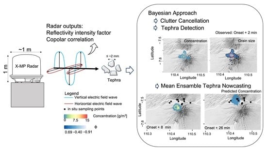
Real-Time Tephra Detection and Dispersal Forecasting by a Ground-Based Weather Radar

Abstract

Tephra plumes can cause a significant hazard for surrounding towns, infrastructure, and air traffic. The current work presents the use of a small and compact X-band multi-parameter (X-MP) radar for the remote tephra detection and tracking of two eruptive events at Merapi Volcano, Indonesia, in May and June 2018. Tephra detection was performed by analysing the multiple parameters of radar: copolar correlation and reflectivity intensity factor. These parameters were used to cancel unwanted clutter and retrieve tephra properties, which are grain size and concentration. Real-time spatial and temporal forecasting of tephra dispersal was performed by applying an advection scheme (nowcasting) in the manner of an ensemble prediction system (EPS). Cross-validation was performed using field-survey data, radar observations, and Himawari-8 imageries. The nowcasting model computed both the displacement and growth and decaying rate of the plume based on the temporal changes in two-dimensional movement and tephra concentration, respectively. Our results are in agreement with ground-based data, where the radar-based estimated grain size distribution falls within the range of in situ grain size. The uncertainty of real-time forecasted tephra plume depends on the initial condition, which affects the growth and decaying rate estimation. The EPS improves the predictability rate by reducing the number of missed and false forecasted events. Our findings and the method presented here are suitable for early warning of tephra fall hazard at the local scale.

1. Introduction

Tephra is the fragmented material produced during an explosive volcanic eruption. Once in the atmosphere, the mix of tephra, volcanic gases, and ambient air forms a volcanic plume. Tephra is classified according to its size as volcanic bombs or blocks (D ≥ 64 mm or ϕ ≤ −6), lapilli (2 mm ≤ D < 64 mm or −1 ≥ ϕ > −6), coarse ash (64 μm ≤ D < 2 mm or 4 ≥ ϕ > −1), and fine ash (D < 64 μm or ϕ > 4), where D is the diameter of the particle and ϕ ≡ −log₂ D (mm). Tephra falls can damage buildings and cause disruption to human livelihoods, agricultural production, and other economic activities [1,2,3]. Because of the significance of the hazards posed by a tephra fall, its timely detection and tracking in the atmosphere is very important.

Tephra can be detected and tracked in the atmosphere with ground-based weather radars operating at various wavelengths [4,5,6,7]. Tephra properties (concentration, fall rate, and diameter) have been retrieved by radar using a microphysical model of atmospheric scattering theorem, which assumed that tephra particles have similar characteristics to raindrops [8,9,10,11]. One of the radar applications that has not been explored thoroughly is its use as an extension to an early-warning system of spatial and temporal tephra dispersal. Up to now, only one study has documented the use of a weather radar for early-onset detection and tracking of tephra [6]. In this previous study, the detection of plume onset was achieved by coupling radar and an infrasound instrument. However, tracking of the plume excluded the sources and sink of radar observable [6]. As a result, the tephra plume’s spatial movement (displacement) was monitored, but the observable radar values were constant through time, indicating a persistent presence of volcanic clouds in the atmosphere. A solution for this problem is applying a dynamic advection scheme, widely used for atmospheric precipitation forecasting [6], known as nowcasting [12,13,14,15]. Nowcasting is a spatial prediction method covering minutes to a few hours of rainfall forecasting based on radar advection vectors. This approach can forecast the rotation and deformation of the observed field and has been an essential prerequisite for real-time flash flood forecasting in operational hydrology [13].

Recently, the ensemble prediction system (EPS) has attracted the interest of modellers, as it can increase the robustness of forecasting results [14,15,16]. When applying the EPS, the nowcasting model is run multiple times from very slightly different initial conditions. Zidikheri et al. have applied this approach to the volcanic ash retrieval model to increase the predictability score of volcanic cloud dispersal forecasting for the 2014 Kelud and 2015 Rinjani eruptions [17]. Their study found that poorer prediction skills could result from using shorter time steps and an incorrect threshold of volcanic ash mass load. The later mentioned reason is related to the limitation of satellite monitoring, particularly at lower altitudes and in surrounding and overlying cloud features not involving ash, which could also account for the discrepancies in the low mass load regions [17]. Moreover, the satellite based-volcanic ash retrieval model requires some input parameters, e.g., the atmospheric profiles (pressure, temperature, and humidity), the surface temperature and emissivity, the volcanic cloud geometry (altitude and thickness), and the ash optical properties [18], which can complicate the calculation process. Contrarily, a weather radar scans the atmospheric information near surface level (<3000 m height) and relies on particle scattering theorem. Using solely radar data, some studies have managed to derive the real-time GSD and tephra concentration [8,9,10,11,19]. The radar estimates are valuable parameters in tephra dispersal modelling by the radar nowcasting approach.

This study presents the potency and uncertainty of real-time tephra plume detection and tracking applied to two eruption events of Merapi in 2018. First, we overcome previous limitations of unwanted clutter contaminating radar scanning data [20] by applying an automatic noise cancellation. Then, we coupled the modified tephra-radar retrieved model [8,9,19,20] with the EPS of radar nowcasting. The evaluation was done by comparing the radar-based tephra properties (i.e., concentration and grain size) with ground-based data and satellite imagery. Through this study, the integration of EPS forecast products can contribute to the potential use of weather radar monitoring in the tephra fall early warning system, which is beneficial for local people living nearby Merapi.

2. Methods

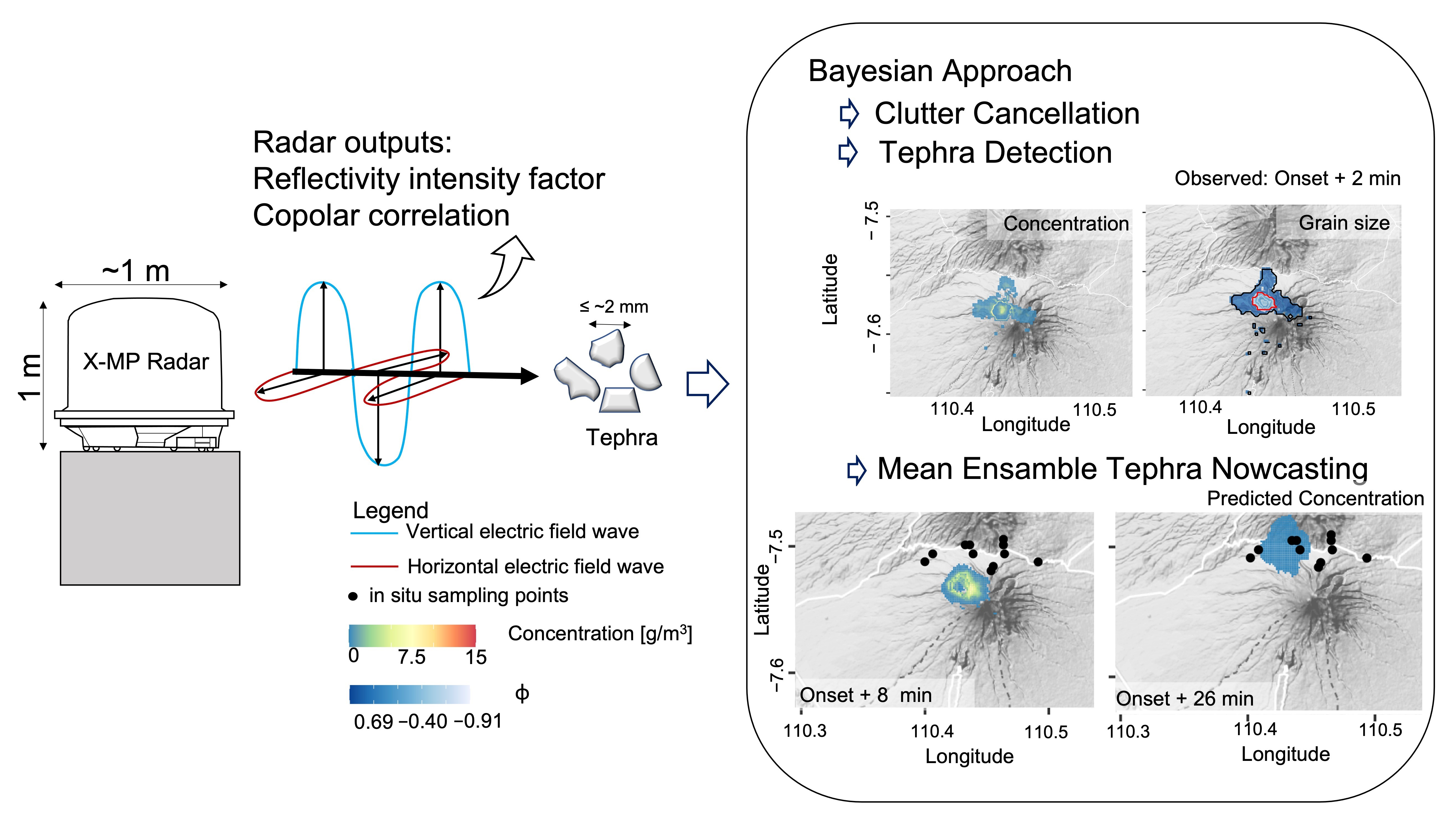
2.1. Radar Setting and Study Case

A small-compact X-band dual-polarization Doppler weather multi-parameter (X-MP) of WR2100 type radar, manufactured by Furuno Electric Co., Nishinomiya City, Hyogo Prefecture of Japan, and was installed and operated at Merapi Museum (7.5 km SW from Merapi’s vent) in 2014–2019 (Figure 1). The main objective of the installation was for research in volcano hazards such as rain-triggered lahar [16,21] and real-time tephra fallout rate [20]. Figure 1 presents the area covered by the 360° radar scan of plan position indicator (PPI) strategy. In PPI scanning mode, the radar scans the volume of the atmosphere by changing the elevation angle in sequence every time it finishes one rotational scan. There were nine different elevation angles: 3, 5, 7, 9, 11, 13, 15, 18, and 21°. An entire volumetric scan sampled the atmosphere into 700 sweeps (beam motion), and each sweep had 300 range gates with a 150 m bin width. It requires 2-min time intervals for a full volumetric PPI scan (all elevation angles). Radar data were heavily affected by ground clutter up to 13° elevation angle scan (Figure 1). While the default clutter cancellation routine by radar can recognize the beam blockage [20], ground clutter may still occur as the result of direct contact between surface and sidelobes owing to the presence of Merapi and Turgo Hill in the SW sector (Figure 1, [20]). Sidelobes are unwanted returns from a direction outside the main lobe, which can bias the reflectivity intensity factor, Doppler velocity, and spectrum width estimates.

Table 1. Radar specification used in the study [27].

Parameter	Description
Transmitter	Solid-state 200 W per channel (H, V)
Polarity	Dual polarimetric horizontal (H) and vertical (V)
Pulses	PRF 600–2500 Hz, Width 0.1–5.0 μs
Antenna	0.75 m ∅, 2.7° beam width
Antenna gain	33.0 dBi
Operating frequency	9.47 GHz
Wavelength	3.3 cm
Peak power	100 W
Scan mode	PPI, CAPPI, RHI
Maximum distance display	50 km
Maximum range fixed observation level	30 km
Data output	(1) Reflectivity intensity factor — $Z_H$[dBZ], (2) Doppler velocity—VD [m s−1], (3) Doppler velocity spectrum width—WD [m s−1] (4) Differential reflectivity –ZDR [dB], (5) Specific differential phase shift—KDP [°km−1] (6) Copolar correlation coefficient—ρ (7) Rainfall intensity—R [mm h−1], (8) Cross polarization difference phase—ΦDP

presents the specification of this small, compact, and light-weighted system. This ground-based weather radar is a dual-polarized system that transmits two different wavelength propagations: horizontal and vertical, giving multiple output parameters, listed in Table 1. Only two parameters were used in this study: the reflectivity intensity factor $Z_H$ and copolar correlation ρ. Reflectivity intensity in horizontal copolar propagation $Z_H$ measures the efficiency of a target to reflect (absorb and re-radiate) radar energy. The copolar correlation ρ is the zero-lag correlation coefficient between horizontally (H) and vertically (V) transmitted and received copolar signals. This parameter shows the uniformity of the features being observed by the radar. Detailed explanations for each of the dual-polarized system’s radar parameters have been discussed in [22]. The $Z_H$ parameter is widely used for tephra classification [8,9,19,20], and ρ produces the least false alarm in unwanted clutter identification [23]. Both $Z_H$ and ρ were used to remove unwanted clutter, and only the filtered $Z_H$ was used for tephra detection and tracking, as explained in Section 2.2 and Section 2.3 and Appendix A.

The selected study cases are two explosive events with the availability of X-MP radar data and in situ tephra grain size information [24], occurring on 11 May 2018 (M05) and 1 June 2018 (M06). Following Merapi’s last centennial explosive eruption in 2010, the volcano experienced six phreatic eruptions between 2012 and 2014. The M05 event was the first minor explosion after four years of quiescence, starting in 2014. It occurred at 00:40 and lasted for 5 min. Time is expressed in hhmm Coordinated Universal Time (UTC). The Centre for Research and Technology of Geological Disasters (Balai Penyelidikan dan Pengembangan Teknologi Kebencanaan Geologi—BPPTKG) officially reported it as a phreatic eruption. Prior to the eruption, there were no unequivocal precursory signals, which is common for this type of eruption. The event produced a 5.5 km high (above its summit) eruption column with explosion energy of 17 MJ [25].

Merapi continued its eruptive activity between 21 and 24 May 2018, by producing multiple explosions. This series of short-lived eruptions ended on 1 June 2018, marked by three explosions that occurred on the same day. The M06 event was the first eruption on that day and had the greatest intensity of the three, occurring at 01:20 UTC for a 2 min duration [26]. The eruption produced a 6 km high eruption column with explosion energy of 46 MJ [25]. Subsequently, Merapi’s activities shifted to be more magmatic, marked by the appearance of a new lava dome in August 2018.

Another reason for selecting these explosive events was the different spatial distributions of the pyroclastic deposit. The deposit of tephra fall from M05 was found in the S sector, while M06 deposits were deposited in the NW sector from Merapi [24]. While being small in magnitude (volcanic eruptive index, VEI-1), satellite images captured both cases (Appendix C: Figure A2), meaning that the reliability of the EPS results could be evaluated.

We used a set of radar data of 56 min, ranging from 4 min before to 52 min after the onset. Hence, it gave a range of time scans at 00:36–01:30 (M05) and 01:16–01:20 (M06). This time range selection was based on visual verification of tephra visibility on radar images. We also found that the plume was only detected at 13–21° elevation angles.

2.2. Tephra Detection

The detection of the volcanic cloud was performed by identifying radar echoes of the tephra from non-tephra echoes. Although both cases occurred during clear days, non-tephra noises still occurred because of sidelobe contamination, anomalous propagation, and the presence of ground clutter. Anomalous propagation results from false radar echoes during calm, stable atmospheric conditions, often associated with super refraction in a temperature inversion, which directs the radar beam toward the ground. We applied a clutter cancellation procedure based on naïve Bayesian classifier to solve the previously mentioned problems [28].

The naïve Bayesian classifier (NBC) is a supervised technique, which implements the classification based on the posterior probability that certain observed measurements correspond to a specific class. In the clutter cancellation process, the unwanted clutters were divided into three classes: the non-clutter data (c = 0), clutter (c = 1), and invalid data (c = −99). The third class was introduced based on the radar signal/beam blocking identified by the Furuno default rain-map program [21]. For our study, only data corresponding to the non-clutter class were recognized as valid and used for tephra detection and tracking.

The 2D spatial data of $Z_H$ were used as the input parameter in the volcanic ash retrieval radar model (VARR, [8,9]). This method is a two-step stepwise approach radar microphysical model, using the scaled gamma distribution. The main assumptions of this method are that tephra particles have a spherical shape and that the scattering of electromagnetic waves follows the Rayleigh theorem [8,9]. Only coarse ash to lapilli regimes were identified by this type of radar [19,20], resulting in two different tephra class regimes: fine (F) and coarse (C) particles. These two terms should be distinguished from finer ash and coarser ash regimes, mentioned in Section 1, as our classification identified class F as a class for particle diameter ranging from 0.015 mm to 0.35 mm and class C for particle diameter ranging from 0.35 mm to 6 mm. This range was generated based on the previous study [8,9,19,20].

Table A1. Input measurements of clutter classification.

${\mathit{Z}}_{\mathit{H}}$	$\mathit{\sigma }\left({\mathit{Z}}_{\mathit{H}}\right)$	$\mathit{z}$
${\rho }_{HV}$	$Pc$

presents detailed information about tephra classification. The clutter cancellation and radar-tephra retrieved model are discussed intensively in [28] and [8,9,19], respectively; hence, only a brief description is presented in Appendix B for convenience. The reproducible code is available in Supplementary Materials.

2.3. Nowcasting and Ensemble Prediction System

Tracking of tephra was performed by adopting the radar’s observable extrapolation model, originally known as the translation model [12]. We assumed radar scan representing the surface level. In meteorology, the radar’s constant altitude PPI (CAPPI) data are widely used to estimate the surface level of rainfall intensity. However, there is no agreement regarding which radar product should be used to estimate tephra properties. Essentially, CAPPI is the 3-dimensional (3D) interpolated data of PPI, and some studies have used this type of data to estimate the tephra fallout rate [20,29]. Meanwhile, other studies have used the lowest PPI elevation angle data to estimate the accumulated tephra deposit [30,31]. In this study, we used the maximum aggregates of radar observable as suggested in [32]. The maximum $Z_H$ is usually related to the densest concentration of tephra [31]. For each 2 min time acquisition of the PPI scan, we calculated the maximum aggregate of tephra concentration across elevation angles of 13–21°. This aggregate value was compiled as gridded 2D (150 m mesh) spatial data. The use of a maximum aggregate was also used to tackle the problem of wavelength sensitivity, which caused the underestimation of retrieved tephra properties [20,33]. Using the tephra concentration, estimated from $Z_H$, we could simplify the forecast of tephra dispersion. This approach did not require the atmospheric condition and ESP information. We used the estimated tephra concentration from the tephra detection framework to estimate the dynamic of its distribution along the x and y directions and time t as follows:

$$\frac{\partial C_a}{\partial t}+m\frac{\partial C_a}{\partial x}+m\frac{\partial C_a}{\partial y}=w$$

(1)

where $m=dx/dt$ and $n=dy/dt$ are radar advection vectors and w = $d{C}_a/dt$ is the radar echo growth and decaying rate (source/sink term). The spatial coordinate (x,y) represents easting and northing UTM, respectively. Variables m, n, and w are defined in Equations (2)–(4).

$$m\left(x,y\right)=c_{1}x+c_{2}y+c_3$$

(2)

$$n\left(x,y\right)=c_{4}x+c_{5}y+c_6$$

(3)

$$w\left(x,y\right)=c_{7}x+c_{8}y+c_9$$

(4)

Ensemble forecasting or EPS could help to get a feeling for the possibilities of pattern evolution. In Equations (2)–(4), $c_1–c_9$ parameters were optimized by linear least square using past estimated tephra concentration, whereas in this case, the first 4–8 min detected plume captured in radar images. Nowcasting could be run according to different phenomena, which led to different ensemble member scenarios (

Table 2. Combinations of advection vectors parameter, adopted from different rainfall phenomena [15].

No	Phenomena	${\mathit{c}}_1$	${\mathit{c}}_2$	${\mathit{c}}_3$	${\mathit{c}}_4$	${\mathit{c}}_5$	${\mathit{c}}_6$	${\mathit{c}}_7$	${\mathit{c}}_8$	${\mathit{c}}_9$
1	Parallel translation			X			X
2	Parallel translation and rotation	X	X	X	X	X	X
3	Rotation	X	X		X	X
4	Parallel translation, growth-decay			X			X	X	X	X
5	Parallel translation, rotation, growth-decay	X	X	X	X	X	X	X	X	X

). Considering the importance of the growth and decay rate to accommodate the sources and sinks of plume presence in the atmosphere, we selected phenomena 4 and 5 in Table 2. For each advection phenomenon, the ensemble member was modelled by various sets of time-lagged forecasts starting at different initial times [34]. As the first visible plume on radar imageries occurred simultaneously at the eruption onset and considering the importance of past observed radar data in generating the advection scheme, the selected initial condition was then decided at 4, 6, and 8 min after the reported onset. Thus, each case had six members, and its subsequent times were separated by 2 min intervals. The nowcasting model was run up to 44 min after the eruption onset, as it followed the presence of detected plume in observed radar data. The mean ensemble was obtained by calculating the mean of all members, using the time average of spatial data at each point (x,y). All results were projected and visualized in WGS 84 coordinate system by rgdal and ggmap libraries of RStudio [35,36].

2.4. Evaluation

The reliability of a predictive approach that considers uncertainty was examined, visually and quantitatively, through the verification of those members and observation from radar and Himawari-8. The observed concentration was derived from the valid $Z_H$ data, i.e., the filtered data after removing unwanted clutter. Himawari-8 is a satellite operated by Japan Meteorological Agency (JMA) since 2014, which observes the earth from 80° E to 160° W and between 60° N and 60° S. The Advanced Himawari Imager (AHI) is an optical radiometer onboard the Himawari-8. Its full-disk observation covers 16 spectral bands from visible to infrared (IR) wavelengths. The spatial and temporal resolutions are 2 km and 10 min, respectively [37]. We assumed this setting caused the Himawari-8 data to be at least 10 min behind radar data or real-time. The standard Himawari-8 data were retrieved from the P-Tree system, managed by the Japan Aerospace Exploration Agency (JAXA) Earth Observation Research Centre (EORC) and JMA. This study used the temperature band difference of band 13 (BTD_B13) as the red beam of BTD_B13–B15 was found to be effective for detecting dust and volcanic ash [38]. The identified tephra plume was defined by lower than 285 K cloud temperature above the coordinates of Merapi, which is the temperature at 3–5 km asl height. The 2D gridded data of Himawari-8 were then transformed into a polygon to delineate the fraction of cloud identified as tephra plume.

Two widely used dichotomous indices were applied: the critical success index (CSI) and the probability of detection (POD). They were given by the following formulas (Equations (5) and (6)), along with a confusion matrix presented in

Table 3. The 2 × 2 confusion matrix [39].

2 × 2 Confusion Matrix		Event Observed
		YES	NO
Event Forecast	YES	Hit	Miss
	NO	False	Hit

. Here, $N_{hit}$ is the number of hit events from the contingency table, $N_{miss}$ is the number of miss events, and $N_{false}$ is the number of false events as defined in Table 2. The values of these indices have the range 0–1, where “1” represents a perfect forecast.

$$CSI=\frac{N_{hit}}{N_{hit}+N_{miss}+N_{false}}$$

(5)

$$POD=\frac{N_{hit}}{N_{hit}+N_{miss}}$$

(6)

Regarding probabilistic prediction, to date, the most common metric for assessing accuracy is the Brier score [40]:

$$BS=\frac{1}{n}{\displaystyle \sum }_{k=1}^n{\left(y_k-o_k\right)}^2$$

(7)

where y is the fraction of members that forecast the event, o is the actual outcome of the event (“1” if it occurs and “0” if it does not occur), and n is the number of forecasting pairs that are spatial. The score of a perfect forecast was “0”. This index was applied to assess probabilistic tephra concentration nowcasting that was equal to or greater than 0.01 g/m³. This threshold equalled the lower limit of generated synthetic data (

Table A2. Statistical properties of synthetic tephra (modified from [9]).

Concentration (g/m3)		Diameter of Particle Classes (mm)
		Fine Class (F)		Coarse Class (C)
		Mean	Range	Mean	Range
		0.10	0.015–0.35	1.00	0.35–6
Light (L)	Mean	0.10		0.10
	Range	0.01–0.50		0.01–0.50
Moderate (M)	Mean	1.00		1.00
	Range	0.50–2.00		0.50–2.00
Intense (I)	Mean	5.00		5.00
	Range	2.00–10.00		2.00–10.00

).

3. Results

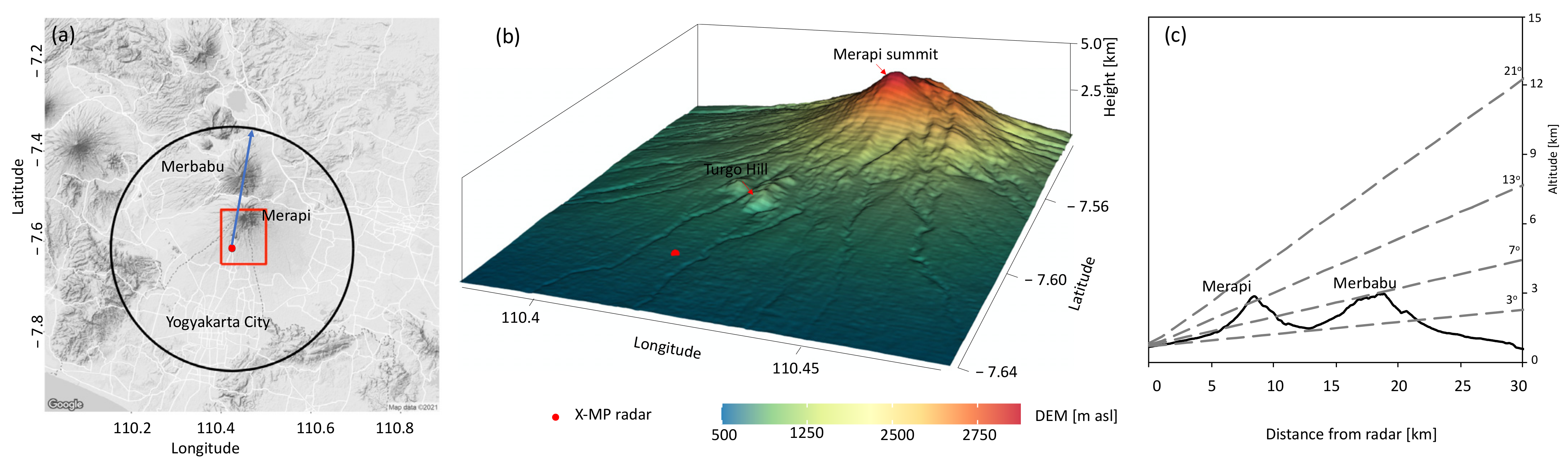
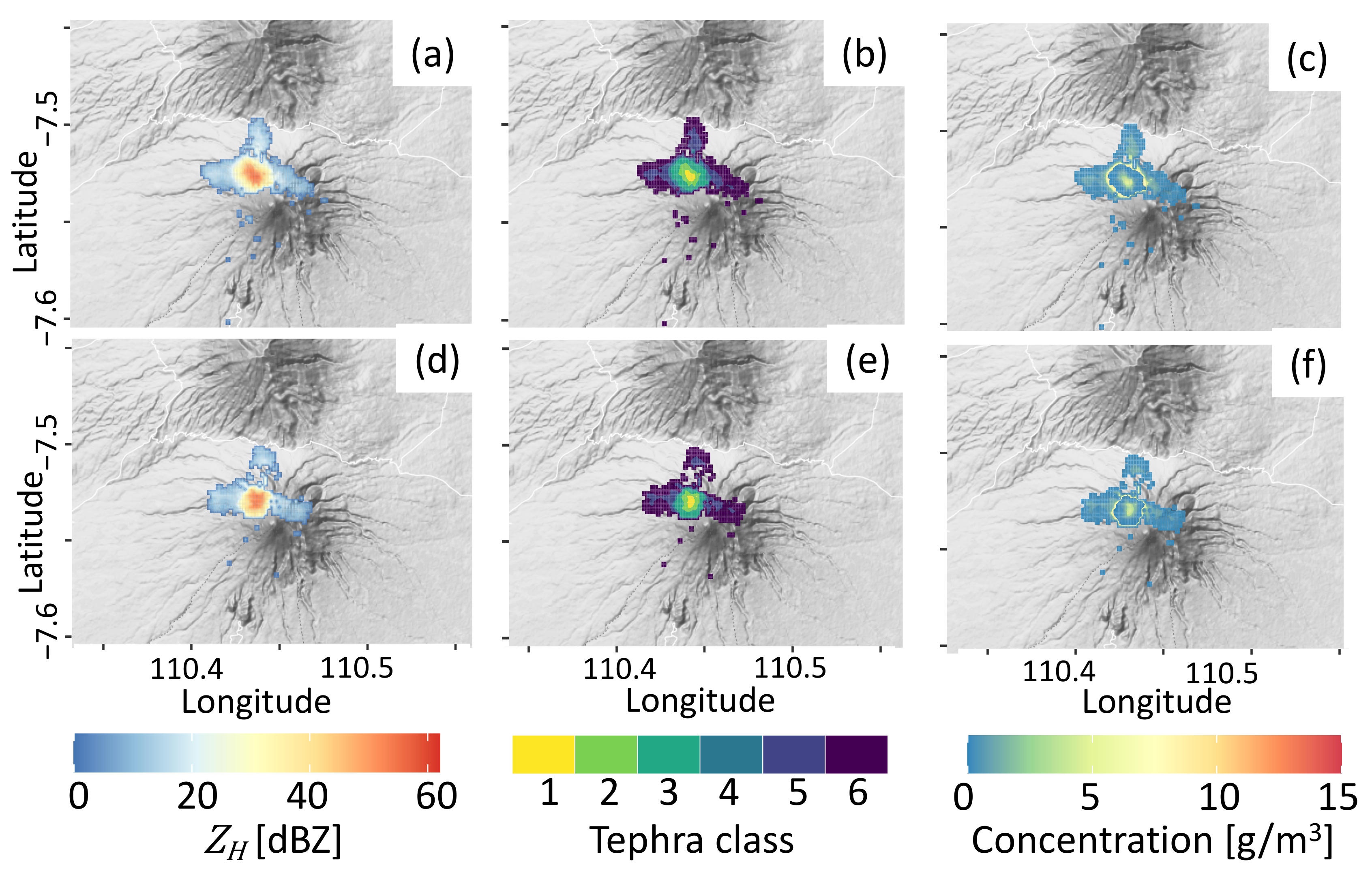
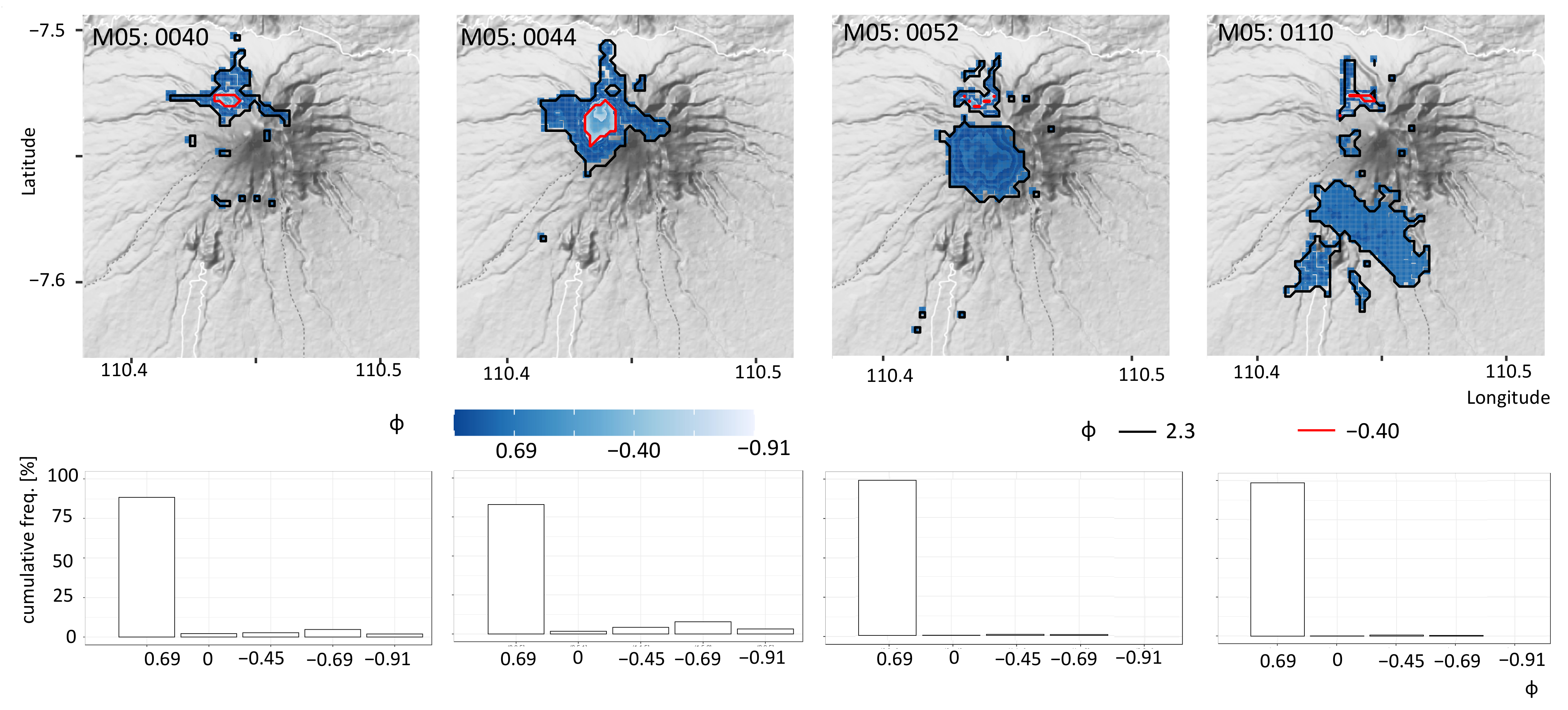
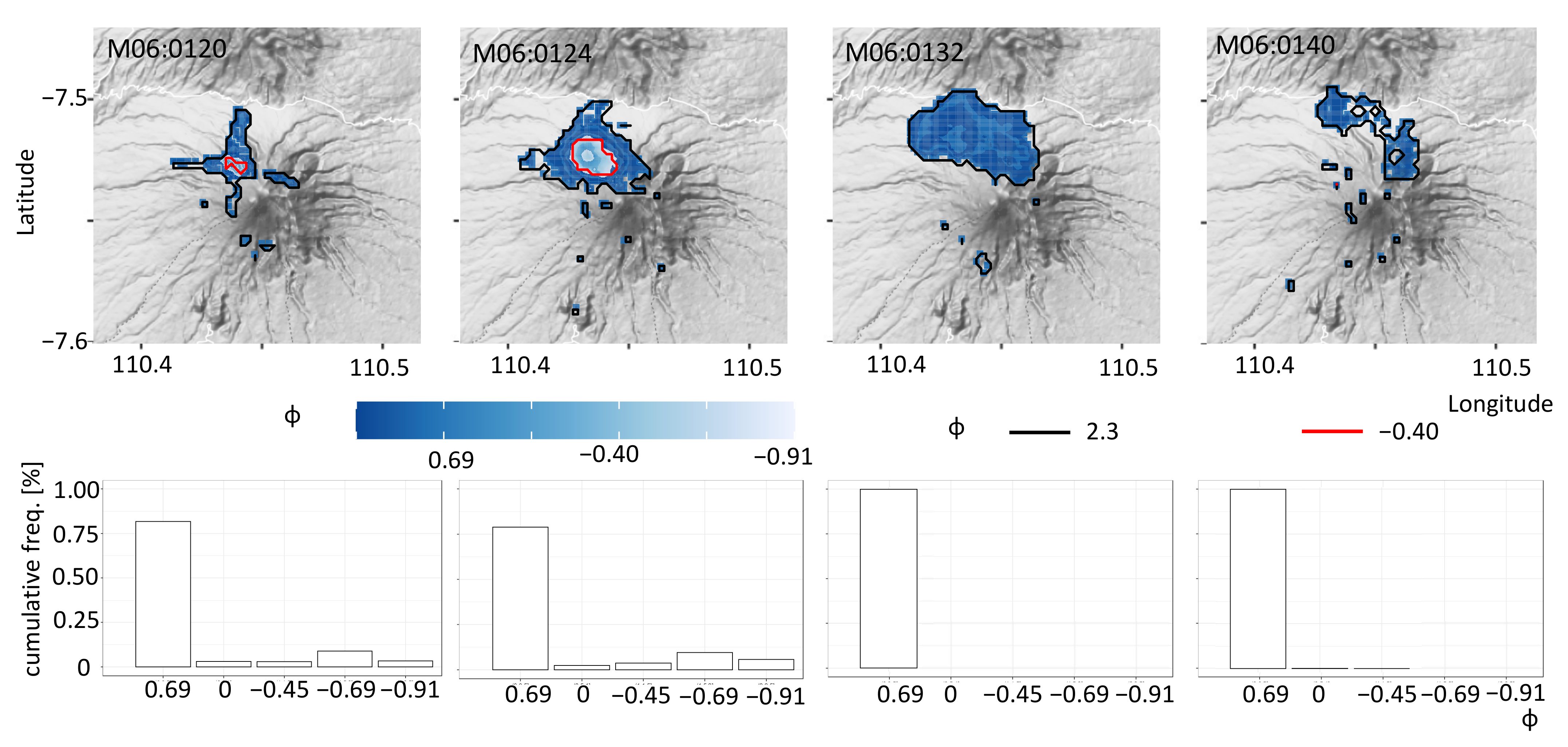
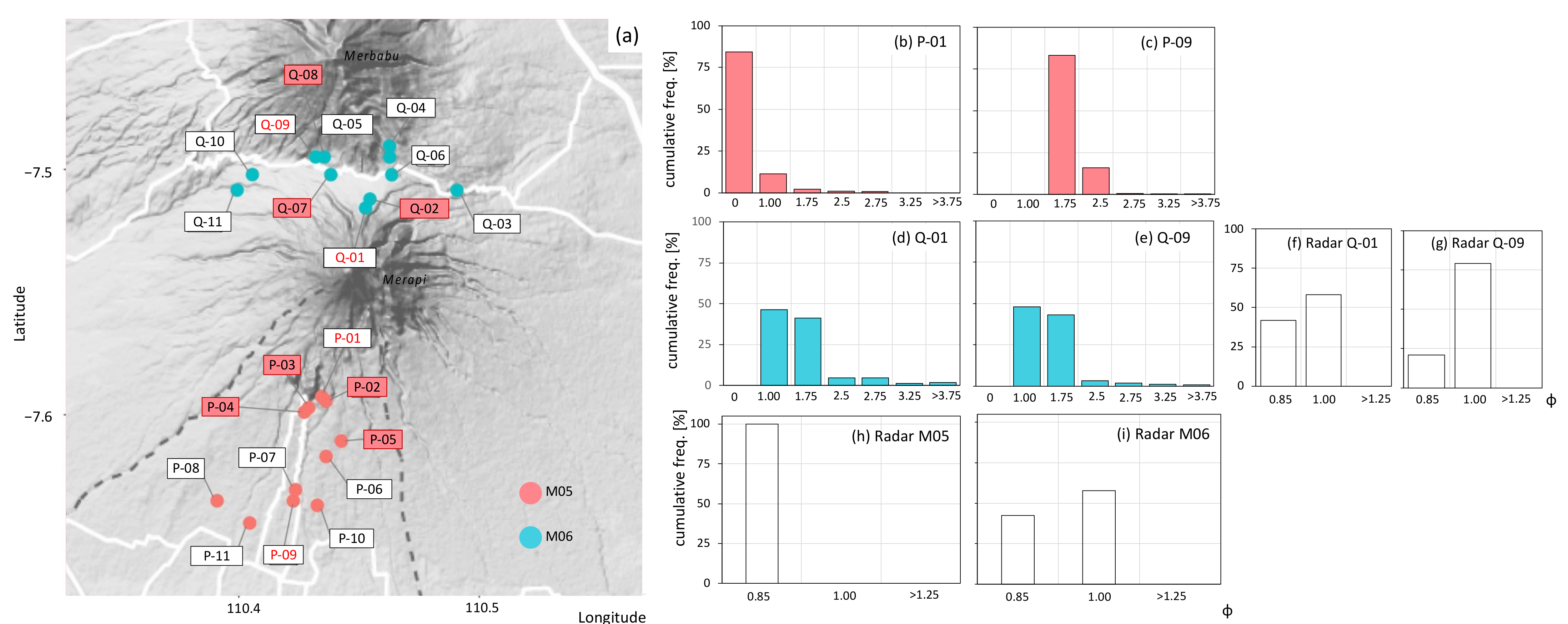
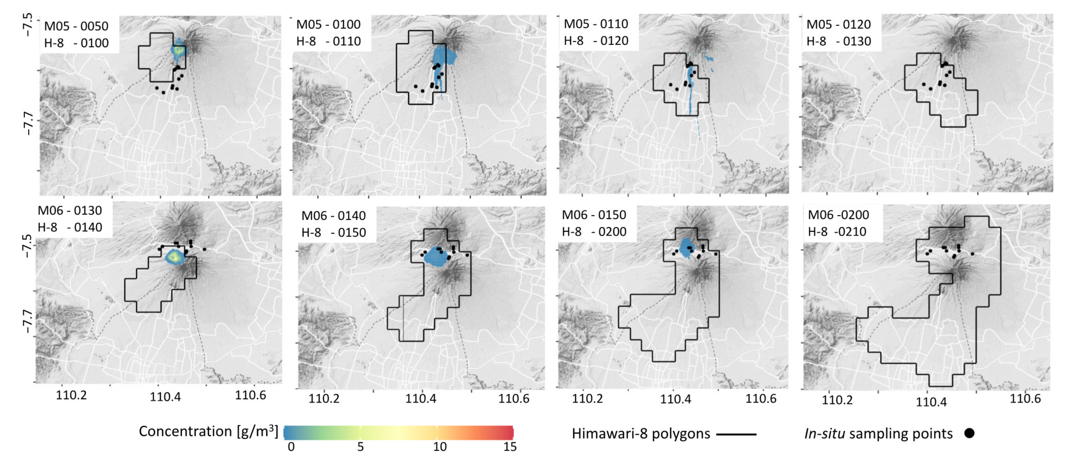
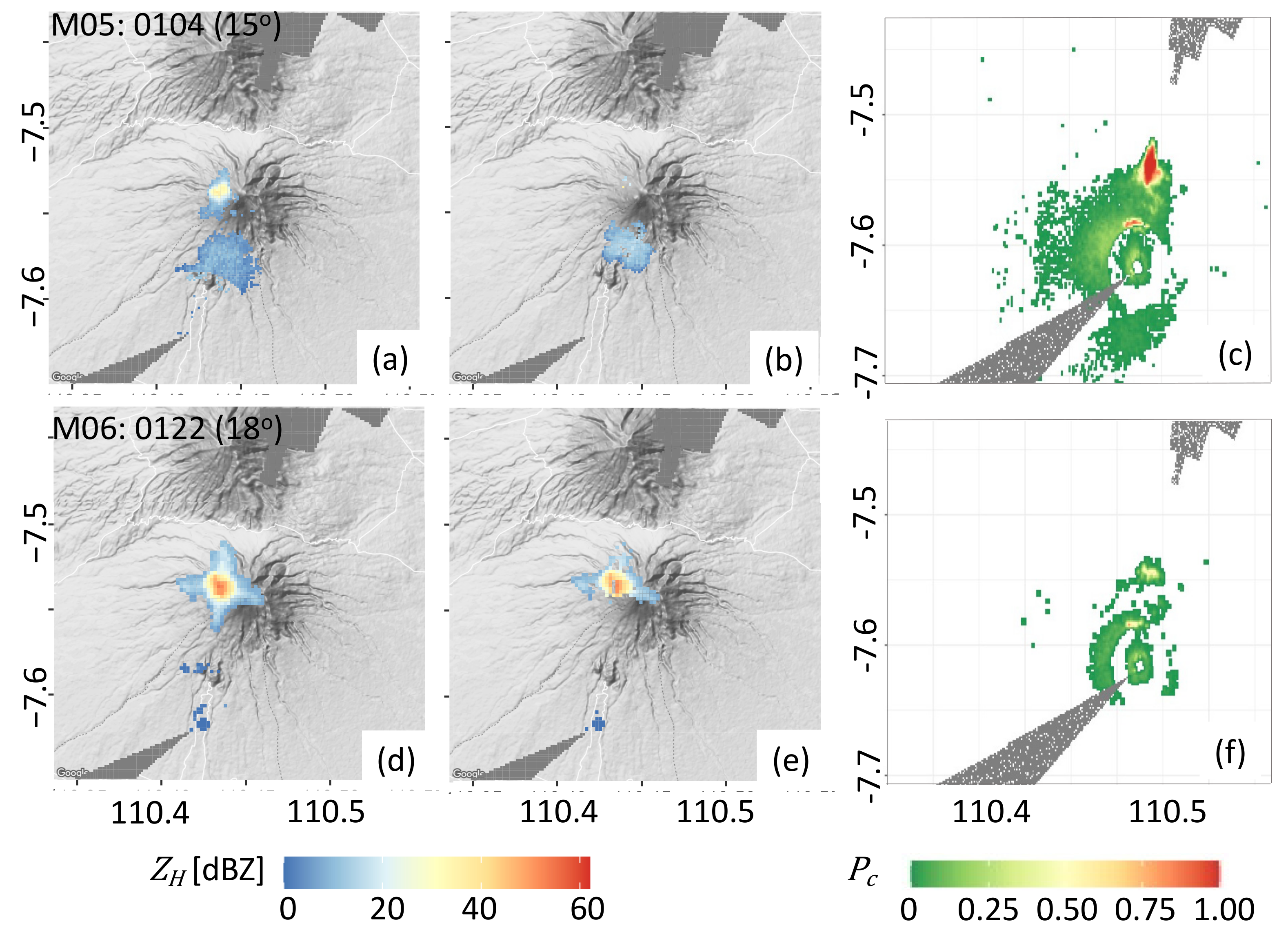
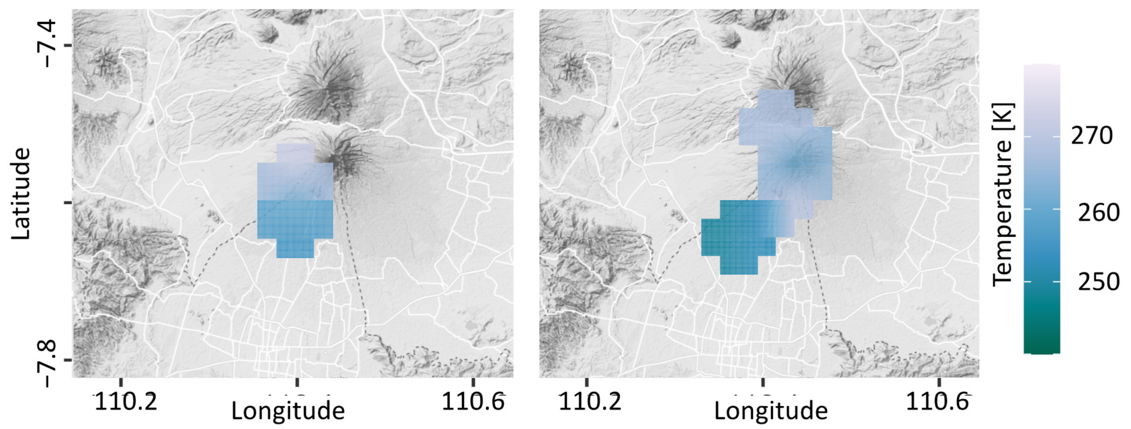
3.1. Volcanic Ash Detection

Figure 2 shows the results of the Bayesian classifier for tephra detection on M05 and M06 at 2 min after the onset. All used $Z_H$ were cleaned from unwanted clutter by NBC, given by some examples presented in Figure A1. All particle size classes (ash and lapilli) were identified at the onset of the eruption. The highest $Z_H$ regimes (>50 dbZ) were associated with the coarse class with the most intense concentration of $C_a$ > 7.5 g/m³. Relatively equal $C_a$ was also obtained by finer class of intense concentration, although it was given by ~35 dBZ $Z_H$.

The spatial and temporal evolutions of radar-retrieved tephra grain size at selected time stamps are given in Figure 3 and Figure 4. For both cases, plumes were identified from 0 min after reported onset up to more than 40 min and 20 min after onset, respectively. The radar-retrieved tephra had particle diameters ranging from 0.02 to 2.3 mm or ϕ = 1.7 to −0.83 (Figure 3 and Figure 4), indicating the limitation of the used X-MP radar in detecting finer particle regimes. Particles larger than 2 mm (lapilli regime) were retrieved from $Z_H$ until up to 4 min after the onset (Figure 3 and Figure 4).

Grain size distributions (in ϕ) of the tephra deposits at sample sites near the volcano [24] and the extracted from the radar retrieved model are presented in Figure 5. We extracted the radar-retrieved GSD at Q-01 and Q-09 and found the spatial distribution of estimated GSDs were relatively in agreement with in situ sample-based data. We extracted more coarser particles’ regimes (ϕ = 0.85–1.0) of the radar-based model at Q-01 (closer to the source) than at Q-09 (distant to the source). About 80% of radar-retrieved GSD at Q-09 was finer particle regimes, ϕ ranging from 1.00 to 1.25 (Figure 5c). For M05, the in situ data points in [24] were available at P-01 and P-09. Unfortunately, the retrieved GSD from $Z_H$ did not produce any data from these two points. The $Z_H$ parameter at those points was probably eliminated following the unwanted clutter removal (Figure 2c,d and Figure A1). However, we could retrieve GSD from P-02 to P-05 and merge their values to represent the GSD for M05. P-02 to P-04 are close to P-01, indicating the extracted GSD at P-02 to P-04 may fall within the GSD range to P-01. P-05 is a few km away from P-01 and the source, so it might produce a finer GSD regime than P-01. Combining all available extracted values at P-02 to P-05 may help characterize the GSD of M05. In Figure 5d, the merged radar-retrieved GSD of M05 is coarser than M06, where 100% of them fall within the range of 0.85–1.0 ϕ.

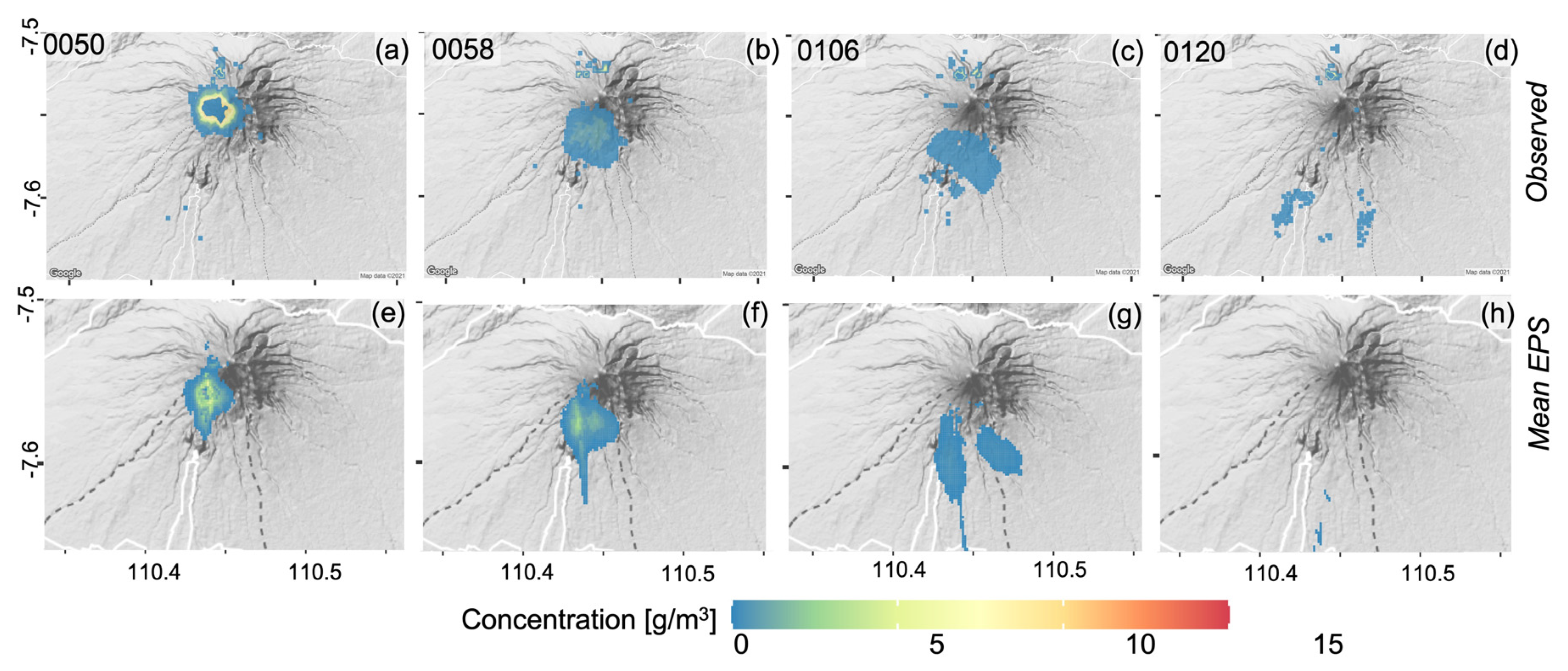
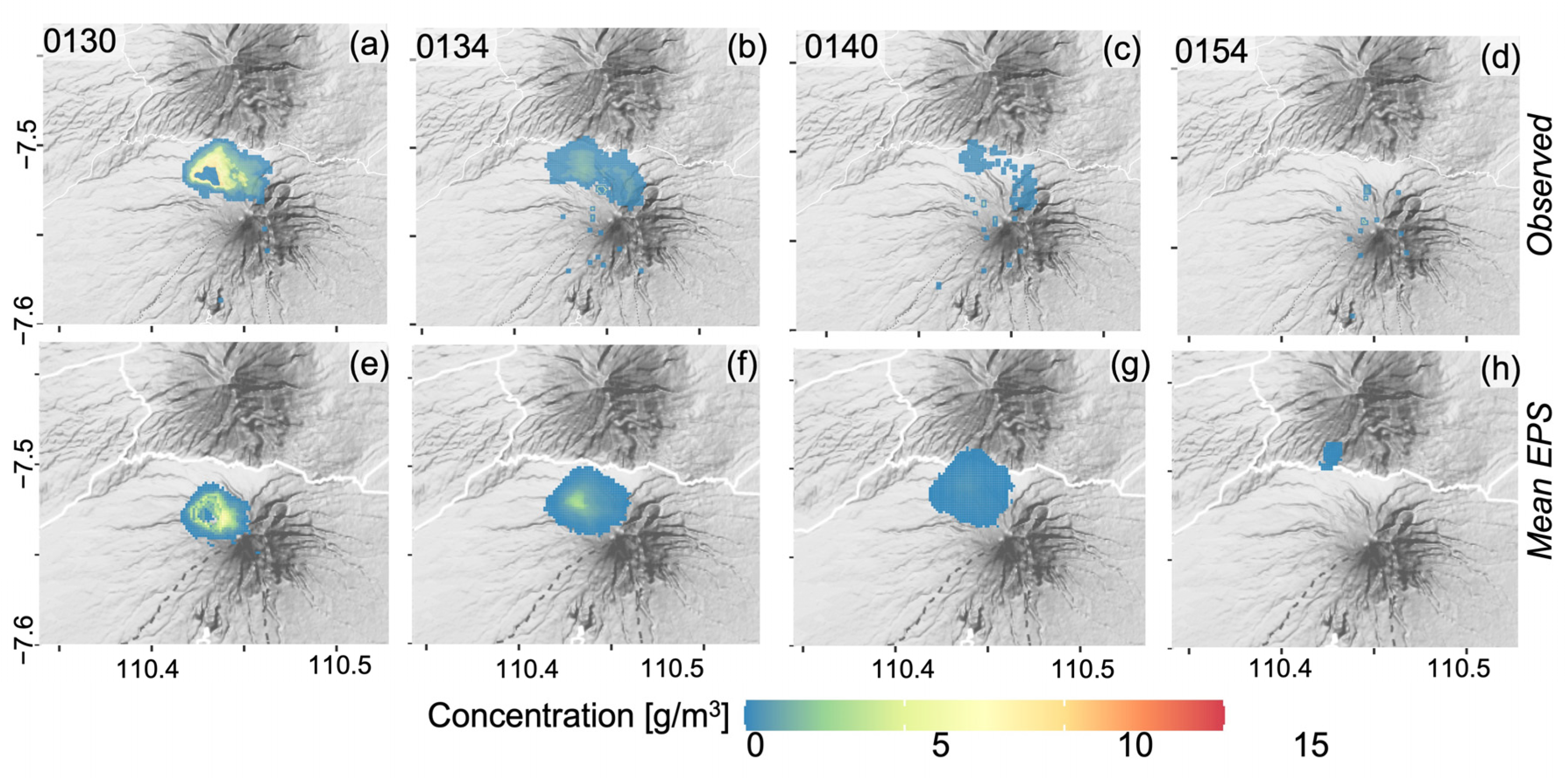
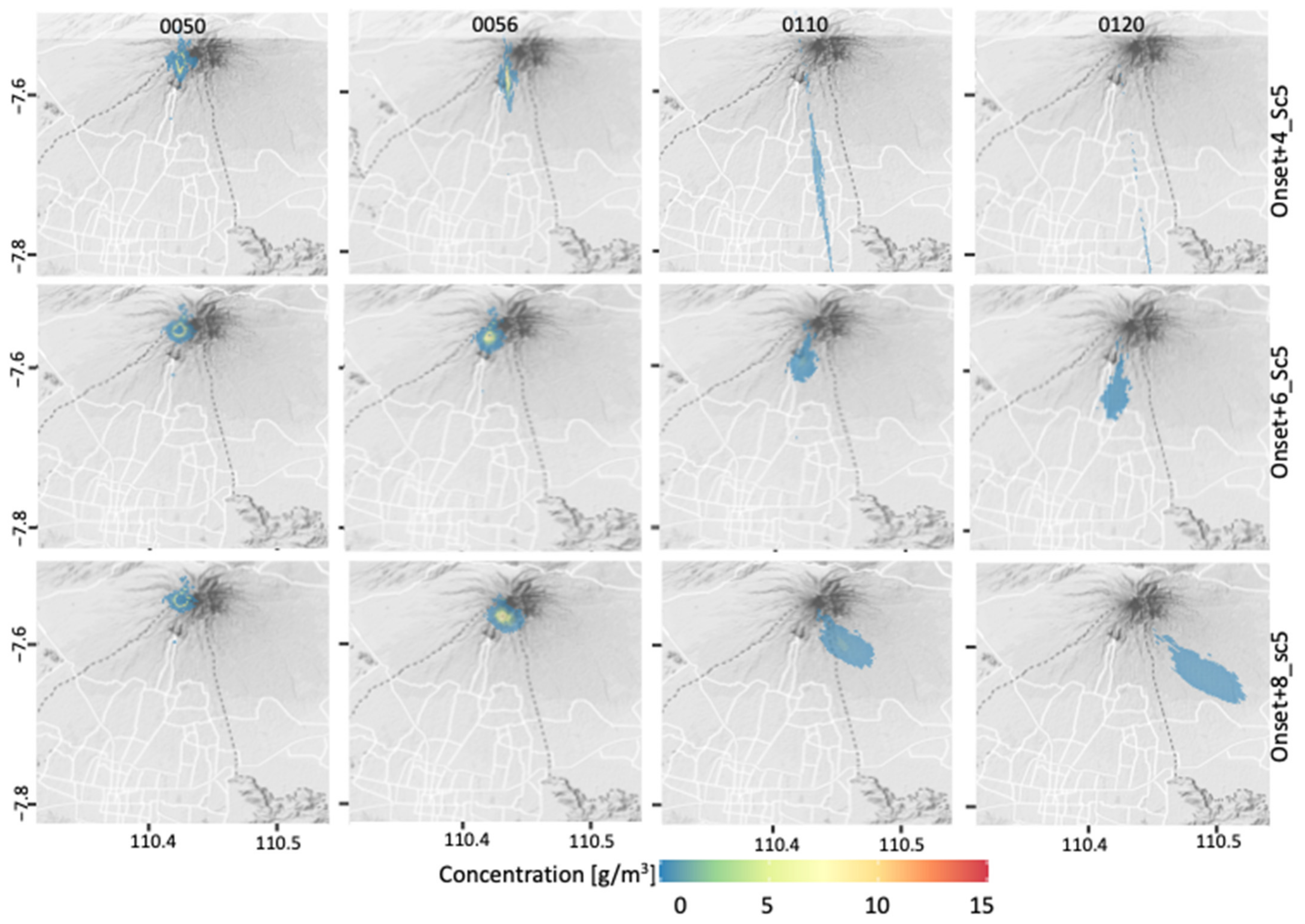
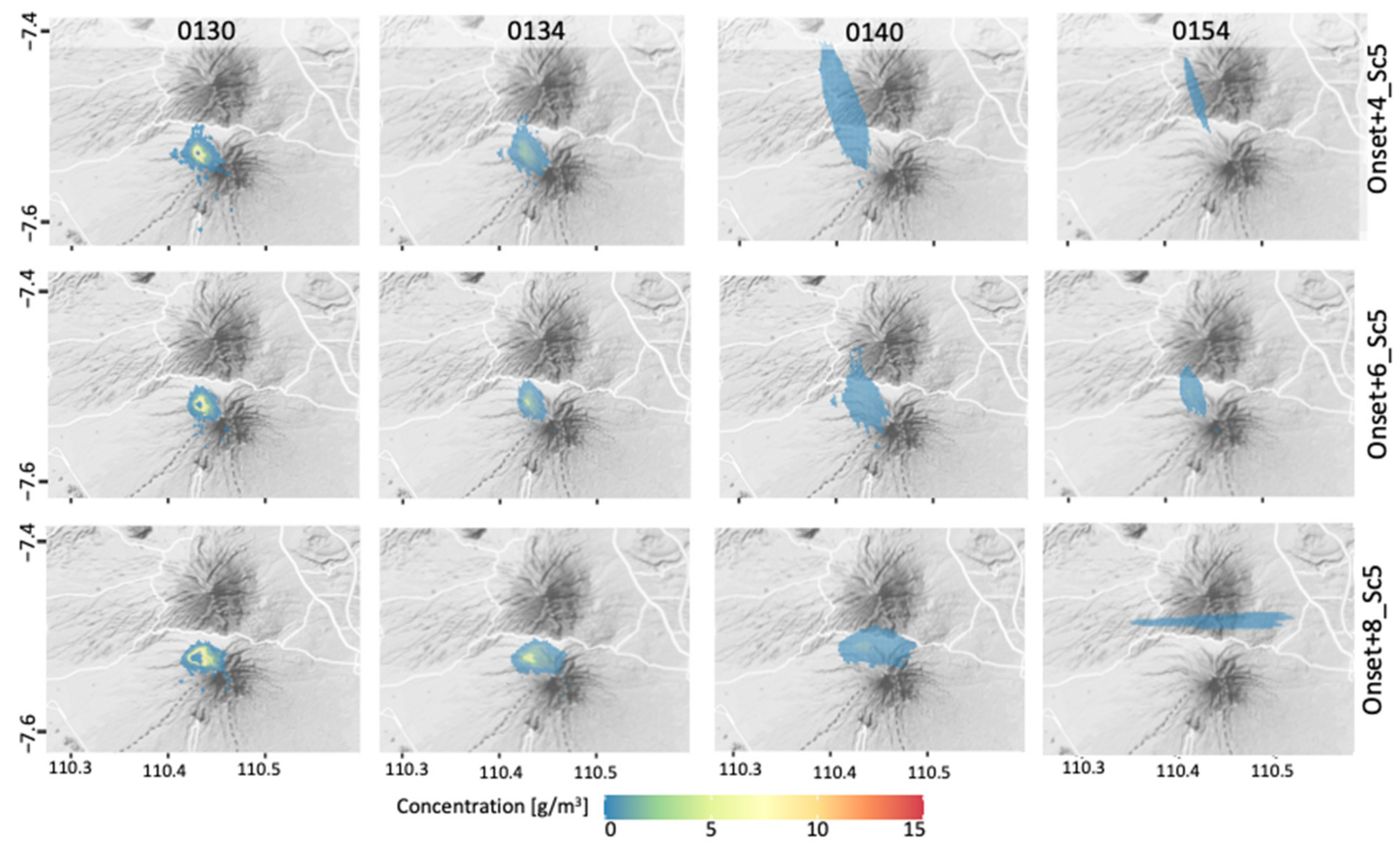
3.2. Forecasting of Plume Dispersion

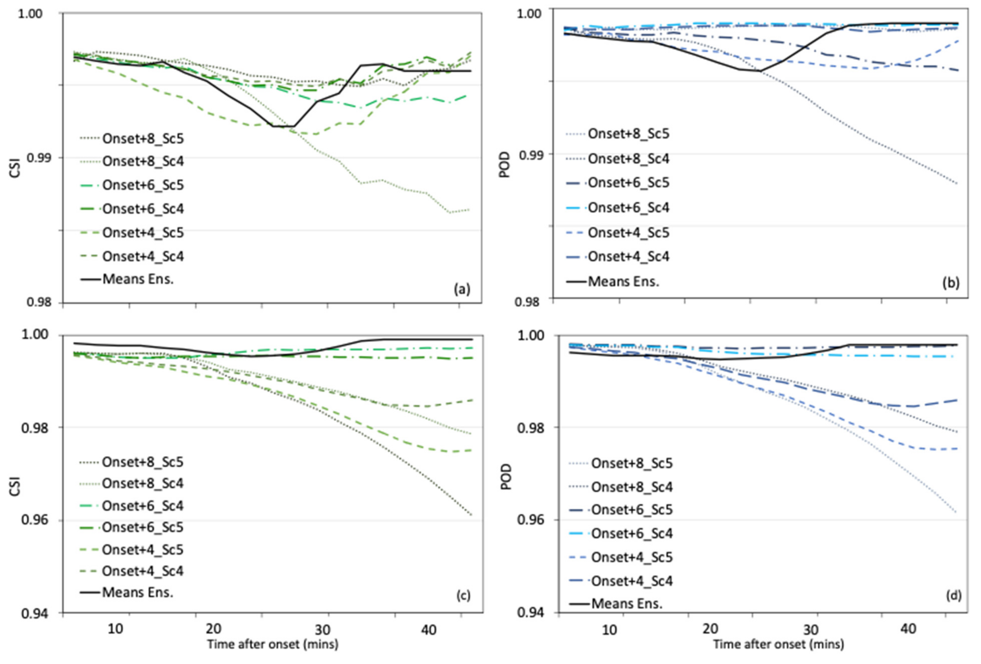
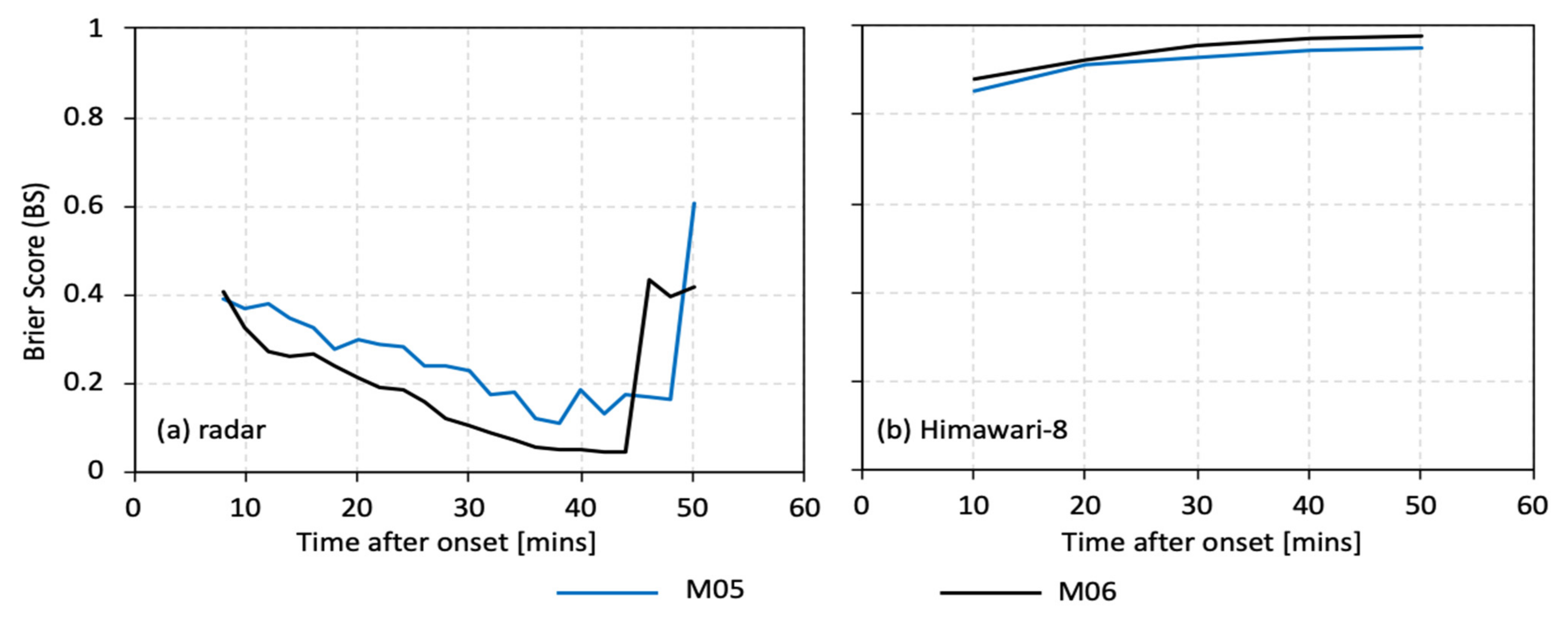
Figure 6 and Figure 7 present the 2D nowcasting tephra concentration results of plume dispersion. Figure A3 and Figure A4 (Appendix C) present some of the ensemble members of nowcasting scenarios of M05 and M06, respectively. The presence of higher than 0.01 g/m³ $C_a$ plume by mean EPS agrees with the retrieved $C_a$ observable from the radar, where their visuals disappear at almost the same time. More than 90% of tephra in M05 disappear 30 min after the eruption onset. Mean EPS and estimated $C_a$ of M06 are unseen at 24 min after the onset. The forecasted $C_a$ of M05 becomes deviated at 01:06, presented by some part of the plume going SE, while the other part is elongated to the S sector. Part of the plume moving to SE sector in M05 is given by the Onset+8_Sc5 (Figure A3). On the other hand, the forecasted EPS plume of M06 consistently dispersed in a circular shape and followed the displacement of radar retrieved $C_a$. Both EPS and radar-retrieved $C_a$ agreed that greater than 5 g/m³ $C_a$ existed for less than 10 min in the atmosphere.

3.3. Evaluation

The predictability scores are presented by CSI, POD, and BS. Both CSI and POD are given in Figure 8, while BS is shown in Figure 9. In the case of BS, we also calculated the score by comparing the ensemble members with Himawari-8 data. The area of volcanic ash identified by Himawari-8 overlying the mean EPS results is presented in Figure 8. Predictability indices generally agree that the highest uncertainty was given by the pair of onset+8 min and Sc5 members.

In general, the EPS of M05 has a better predictability rate than M06, according to CSI and POD. On the contrary, the BS of M06 mean EPS is better than M05. However, we consider that BS provides more reliable results for the predictability rate as it only counts pairs of occurrence and non-occurrence events (Equation (5)). The CSI and POD scores decreased over time, but then increased, indicating the failure estimation of correct growth and decaying rate of some members. The cross-validation of the observed radar involving all ensemble members increases the predictability rate until 40 min after the onset, with BS ranging at 0.4 to 0.2. After 40 min, the model performance becomes significantly poorer because of the accumulated error of incorrect growth decaying rate given by some ensemble members. Although all the predictability rate parameters indicate the tendency of skill to decrease with time, we still highlight the importance of EPS in improving the accuracy of the tephra forecast, as it can maintain the CSI and POD to be greater than 0.99 for entire prediction time-steps.

Comparing the temporal and spatial of mean EPS to Himawari-8 data (Figure 10) gives the impression that the use of weather radar is limited in detecting the finest regime of the plume. The radar-based EPS did not give the same spatial tephra distribution as Himawari-8 data, especially in the S sector. However, the EPS modelled the displacement of the plume that matched with the in situ sampling points better than Himawari-8 data (Figure 10). In Figure 9b, the cross-validation of the ensemble members with cloud temperature (Himawari-8) gives BS ranging from 0.85 to 0.90 within the first 20 min after the onset. Ten minutes later, the predictability skill becomes poorer, given by greater than 0.95 BS.

4. Discussion

4.1. Tephra Detection

Applying unwanted clutter cancellation is an important step in radar data processing. Here, we presented a simple procedure that could be easily included in the radar processing routine. In

Table A3. Contingency table of clutter classification by NBC.

Class		Clutter	Non-Clutter	Invalid
Elevation angle 3°	Clutter	0.90	0.06	0.00
	Non-Clutter	0.10	0.94	0.00
	Invalid	0.00	0.00	1.00
Elevation angle 5°	Clutter	0.96	0.04	0.00
	Non-Clutter	0.04	0.96	0.00
	Invalid	0.00	0.00	1.00
Elevation angle 7°	Clutter	0.98	0.04	0.00
	Non-Clutter	0.02	0.96	0.00
	Invalid	0.00	0.00	1.00
Elevation angle 9°	Clutter	0.98	0.03	0.00
	Non-Clutter	0.02	0.97	0.00
	Invalid	0.00	0.00	1.00
Elevation angle 11°	Clutter	0.99	0.03	0.00
	Non-Clutter	0.01	0.97	0.00
	Invalid	0.00	0.00	1.00
Elevation angle 13°	Clutter	1.00	0.03	0.00
	Non-Clutter	0.00	0.97	0.00
	Invalid	0.00	0.00	1.00
Elevation angle 15°	Clutter	0.95	0.02	0.00
	Non-Clutter	0.05	0.98	0.00
	Invalid	0.00	0.00	1.00
Elevation angle 18°	Clutter	0.99	0.30	0.00
	Non-Clutter	0.01	0.70	0.00
	Invalid	0.00	0.00	1.00
Elevation angle 21°	Clutter	1.00	0.10	0.00
	Non-Clutter	0.00	0.90	0.00
	Invalid	0.00	0.00	1.00

, an elevation angle 18° had the highest probability of misclassification (p = 0.3), while other elevation angles performed relatively better (p ≤ 0.1). The misclassification can reduce the numbers of $Z_H$ s associated with tephra. As presented in Figure A1, a significant number of $Z_H$ pixels in the SW and NW sectors of M06 were removed at elevation angles of 15°and 18° after applying the NBC. Aggregating the $Z_H$ (max) from elevation angles of 13–21° helped restore most of the data in the NW, but was still unable to reserve the echoes in the SE sector (Figure 2). This limitation is the consequence of a higher frequency of clutter in the SE sector. When the radar was pointing to the Merapi vent, the sidelobes were in contact with the hill side of Merapi (Turgo Hill, Figure 1b), producing unwanted radar noises in this sector.

Larger than 2 mm diameter particle (ϕ < −0.69) lasted only four minutes after the eruption in the atmosphere. This tephra regime was part of the eruptive mixture in the early development stages [41]. It should be noticed that larger and finer particles than the estimates may occur, unmonitored by the current method owing to the limitation of radar-retrieved GSD. The limitation is mainly related to radar specification (e.g., antenna gained, wavelength, radar sensitivity, and scanning speed). Larger tephra particles also fall faster, and such speed might be unmonitored by the 2 min temporal resolution of scanning radar. Moreover, some studies in tephra retrieval by the microphysical model of radar also found that intense tephra concentrations can be associated with greater amounts of finer and slower falling particles within a sampling volume [9,19,20].

As noted earlier, we failed to extract radar estimates of GSD for M05 at two radar sampling points with available information of in situ data (P-01 and P-09, Figure 5). We could only extract the radar-retrieved GSD at some points near P-01. Notice that the in situ sampling points in Figure 5a were collected on surface level, while the radar-based model estimated the GSD at elevation angles of 13–21° scans. Although this study assumed the observed radar parameters could represent the surface level, there was still uncertainty owing to atmospheric condition (i.e., wind profile) affecting the tephra distribution. Hence, some of radar images could not align well with the in situ data points [24]. While this study confirmed the incomparability between atmospheric and surface level data, we could use the grain size collected on ground data to constrain and compare the range of grain sizes inferred from radar. Point Q-01 and Q-09 are close and distal to the vent, respectively, and thus reflect the end members of the GSD for the whole sample region. However, based on the conclusion in [24], there was no significant difference between the sortation in both points, where they categorized the GSD to be moderately well sorted. The extracted radar-retrieved GSDs have limited distribution, where ϕ = 0.85–1.25. This limitation is related to the Rayleigh scattering theorem used in this study, which limits the 3.3 cm wavelength of radar to be associated with smaller than ~2 mm mean particle diameter. Within the limited GSD range, our study could capture the spatial change in GSD, where the number of coarser particles decreases at a distant point from the radar. As presented on Figure 5e, Q-01 has a greater portion of coarse GSD than Q-09. Our estimates match the broadly predictable feature of GSD, which is a decrease in mean particle size with distance from the vent [42].

While the estimated GSD from the radar-retrieved model was slightly greater than the in situ data (for M06), the majority of radar-retrieved GSD fell within the range observed in [24] (Figure 3). More importantly, the radar-retrieved estimates of particle size also agreed with the conclusion of [24], that the tephra from M05 had a coarser grain size than M06 (Figure 5h,i). The difference between GSD for the two case study events can be attributed to the level of the eruption’s explosivity and surface energy consumption. An eruption with lower explosion energy (M05) produced coarser grain pyroclastic deposits than the higher explosion energy (M06) [43,44]. However, it should be noted that the prediction of GSD from explosion energy is still an active area of research, and the variety of fragmentation processes and magma properties makes it difficult to construct a general relation between GSD and energy balance [44].

4.2. Forecasting the Dispersal of Tephra

Spatially, the mean EPS could track elevated tephra concentrations estimated by observed and valid $Z_H$. The initial conditions used have a significant role in the estimated tephra dispersal, where the longest and shortest time windows tend to have poorer predictive skills. The shortest time window (onset+4) members show the tendency of the tephra cloud to elongate in the y-direction (N–S), as it could not estimate the correct horizontal u-wind component (parallel to the x-axis: E–W), as presented in Figure A3 and Figure A4. This signature is more visible in M05 than in M06, where the forecasted plume elongated in the NS direction (Figure 6 and Figure 10). The plume expansion in the NS direction could also be attributed to the vertical growth or decaying rate, as it showed the change in altitude along with the range distance. As the radar is located in the SW sector, the altitude of the radar scan increases with radar’s range in the N sector. The aggregated maximum $Z_H$ from different elevation angles (13–21°) may represent the actual growing or decaying rate at a different height. The ejected material with a higher concentration would have reached a higher altitude before expanding horizontally within a shorter period (onset+4). This result explained the more intense concentration estimates in the NW sector for both cases. Hence, the translation model might have calculated an increasing trend of $Z_H$ along the y-direction (NS), resulting in the NS elongated orientation of plume expansion. On the other hand, the most extended time window (onset+8) members showed an expansion of the plume to the u-wind component, indicating underestimation of the growth and decaying rate (Figure A3 and Figure A4). At this time window, the identified plume had lost most of the intense $Z_H$ regime (>45 dBZ), causing an exaggeration of horizontal expansion.

Additionally, unlike precipitation, the advection vectors that determine the rotation and translation of tephra displacement were generated from fewer sample points, resulting in a higher error rate. Despite these limitations, this method has confirmed the time-dependent plume evolution exhibited in short-lived Vulcanian eruptions [45]. We confirm a recommendation by a previous study [17] stating that, for EPS, the use of past data started too soon from the onset results in inferior predictive skill. However, it may also depend on the magnitude of eruption and the temporal scale of the instrument. As presented in this study, both cases are small-scale explosive events producing short-lived volcanic plumes. Generating the nowcasting using past data of the shortest (onset+4) and longest (onset+8) time window produces poorer results than using onset+6 as the initial condition. A longer time window, up to 6 h from the onset, was recommended in the satellite-based ensemble prediction of volcanic ash dispersal from the VEI-4 Kelud eruption [17]. This longer time window is not applicable for the short-lived plumes analysed by this study. For our study cases, onset+6 can probably better cover both the plume expansion (related to the energy release and ESP) and wind components (Figure 8, Figure A3 and Figure A4).

In the future, applying this method to larger magnitude eruptions will help answer the uncertainty of the optimum lead time applied to the nowcasting of the volcanic ash dispersal. A plume generated from a larger scale and more extended duration eruption event may last longer in the atmosphere and cover a broader area in the radar’s azimuth display, enabling the addition of ensemble members for a more robust forecast. However, the forecast can be more challenging in the case of successive explosive pulses as they may not be suitable for a linear approach used in this study. Optimizing the nowcasting approach by the deep learning method has been considered effective in improving forecast quality. This method can solve non-linear precipitation phenomena, such as convective initiation [46].

The mean EPS can reduce the uncertainty of forecasted tephra track, spatially and temporally (Figure 6, Figure 7, Figure 8 and Figure 9). Mean EPS took consideration from the mean values of ensemble members with $C_a$ > 0.01 g/m³. Hence, it removed the lowest probability forecasts, resulting in more reliable results that matched the estimated $C_a$ from radar observable. As EPS reduces the uncertainty of forecasts, it significantly improves prediction skills. In Figure 8, even though both CSI and POD show a typical behaviour of nowcasting, where it decreases following the time increase, the mean EPS maintained the prediction skill relatively better than ensemble members.

Estimating the growth and decaying rate for M06 is probably more challenging than M05, as given by CSI and POD scores. As the plume goes to the NW sector with a higher altitude, the maximum aggregate may contain higher $Z_H$ values (corresponding to higher $C_a$). Consequently, it produces more variability in the data distribution, which results in a higher error rate when estimating the w parameter of some ensemble members. The poorest ensemble members forecast is given by combining all phenomena: parallel translation, rotation, and growth and decaying rate. The dispersion of the small size plume is mainly related to wind vectors and not by a mesoscale rotational motion, such as the case of a tropical cyclone. However, it should be noted that the higher predictability score given by CSI and POD is based on large numbers of zero-valued pixels. The observed radar range was fixed at 30 km (Table 1) with a 150 m mesh resolution, resulting in significant $N_{hit}$ generated from pairs of zero-valued pixels but insignificant numbers of $N_{false}$ and $N_{miss}$ (Figure A5). Visual verification is crucial to conclude if each ensemble member can correctly imitate the tephra plume’s movement and expansion.

Plume in M06 can maintain its circular shape that followed the radar-retrieved $C_a$, while plume in M05 has an elongated shape that does not match the radar-retrieved $C_a$. A different result is obtained when comparing the mean EPS with satellite data, where M05 is slightly better than M06. However, the scores are poorer than the comparison made with radar data. Poorer BS given by comparing radar nowcasting and satellite is reasonable owing to the different spatial patterns of the ash cloud seen by the two sensors because of the attenuation of different particle size sensitivity [31]. Himawari-8 infrared observation (λ = 10.4 μm for BTD_B13) is more sensitive to capture finer particles than the X-band radar observation (λ = 3.3 cm). The difference is more noticeable for M06, as the undetected tephra plume of Himawari-8 by the EPS model occurred in the S sector, which has the lowest elevation scanned by radar. M05 has coarse GSD and distributes in the lower elevation within the radar’s scanning range. The radar can observe the displacement in M05, enabling it to be modelled by nowcasting. Conversely, M06 has finer GSD and greater magnitude than M05. This may imply that the ejecta of M06 has greater exit velocity, which potentially helps raise the tephra mass to a higher altitude than M05, exceeding the radar’s observable elevation angles. At higher altitudes, stronger wind shear can benefit the dispersal of the finer GSD of M06 in the S sector, as seen in Himawari-8 images. This regime of particles may also belong to the very-fine far travelling airborne ash mass, which can only be captured by satellites [46].

The detected tephra observed by radar are coarser than the satellite-based model [47], hence it is more likely to fall nearby the volcano because of its higher settling rate. This conclusion is supported by the spatial distribution of mean EPS that matches the distribution of tephra on the ground [24]. The detected plume by Himawari-8, on the other hand, had a much wider distribution within an area that did not belong to the in situ sampling area, especially for M06 (Figure 10). Hence, this study reveals the benefit of the X-band radar for a local early warning system in tephra hazard management, which is essential for the nearby population.

Even though the cloud temperature of Himawari-8 and estimated radar tephra concentration is not equally comparable owing to the difference in resolution, sensor’s wavelength, and observed parameter, we assume that data from both instruments are complementary. Comparing data from both instruments helps differentiate tephra regimes that will fall earlier (ground-based radar) and parts of the finer ash regimes within a plume that may be transported at a higher altitude and potentially cause disruption to aviation (satellite). Moreover, the estimated tephra concentration from the radar is essential information for the characteristic of the plume in the lower altitude, which cannot be retrieved from the satellite data [17]. It also demonstrates the limitation of radar in observing the very fine airborne ash regime, which is captured by satellite.

5. Conclusions

This study has demonstrated the potency of an X-MP radar to detect and forecast tephra plume in Merapi. We estimated tephra concentration and GSD using solely ground-based radar data. We retrieved both tephra properties from two cases of explosive eruption: M05 and M06, based on radar’s $Z_H$. Only valid $Z_H$ was used in the model as unwanted clutters and sidelobes contamination were automatically cancelled by the Bayesian approach. Using the microphysical model of radar, we found that higher than 7.5 g/m³ tephra concentration lasted only 4 min after the onset. M05 has a coarser GSD than M06, which agrees with the in situ data. Applying the radar nowcasting in the manner of EPS reduced the uncertainty of forecasted tephra dispersal. However, the forecasts rely on radar observation with limited wavelength sensitivity and scanning range. Hence, it cannot forecast the very-fine ash regime transported to the higher than radar’s elevation angles observation. Despite this limitation, the spatial distribution of the forecasted plume matches the distribution of tephra on the surface level, enforcing its potency in the early warning system for local people living nearby Merapi.

While more work is needed to apply the remote sensing approach of tephra plume tracking using ground-based weather radar, this study has presented the potential use of a weather radar to forecast the dispersal of tephra. A crucial problem is an uncertainty in estimating the growth and decaying rate. Capturing the dynamic of the tephra plume is challenging. Different eruptive cases may require more ensemble members than the one we presented here, or even different approaches, such as the deep learning method for a more robust forecast.

In order to overcome the limitation of observing only part of the volcanic plume with ground-based weather radar, future work should be more focused on integrating the radar and satellite data through data assimilation. Such a study will solve the classical problem of not detecting fine ash by radar observation while simultaneously improving the efficiency of the volcanic plume estimation by satellite data. This multisensory approach can reduce the complexity of tephra plume dispersion modelling and improve the reliability of its real-time forecasting using remote sensing techniques.

References

1. Williams, G.T.; Jenkins, S.F.; Biass, S.; Wibowo, H.E.; Harijoko, A. Remotely assessing tephra fall building damage and vulnerability: Kelud Volcano, Indonesia. J Appl. Volcanol. 2020, 9, 10. [Google Scholar] [CrossRef]
2. Jenkins, S.F.; Wilson, T.M.; Magill, C.; Miller, V.; Stewart, C.; Blong, R.; Marzocchi, W.; Boulton, M.; Bonadonna, C.; Costa, A. Volcanic ash fall hazard and risk. In Global Volcanic Hazards and Risk; Loughlin, S., Sparks, S., Brown, S., Jenkins, S., Vye-Brown, C., Eds.; Cambridge University Press: Cambridge, UK, 2015; pp. 359–370. [Google Scholar] [CrossRef]
3. Jenkins, S.F.; Spence, R.J.S.; Fonesca, J.F.B.D.; Solidum, R.U.; Wilson, T.M. Volcanic risk assessment: Quantifying physical vulnerability in the built environment. J Volcanol. Geotherm. Res. 2014, 276, 105–120. [Google Scholar] [CrossRef]
4. Donnadieu, F.; Freville, P.; Hervier, C.; Coltelli, M.; Scollo, S.; Prestifilippo, M.; Valade, S.; Rivet, S.; Cacault, P. Near-source Doppler radar monitoring of tephra plumes at Etna. J. Volcanol. Geotherm. Res. 2016, 312, 26–39. [Google Scholar] [CrossRef]
5. Donnadieu, F. Volcanological Applications of Doppler Radars: A Review and Examples from a Transportable Pulse Radar in L-Band. In Doppler Radar Observations-Weather Radar, Wind Profiler, Ionospheric Radar, and Other Advanced Applications; Bech, J., Chau, J.L., Eds.; InTech: Urbino, Italy, 2012. [Google Scholar] [CrossRef] [Green Version]
6. Marzano, F.S.; Picciotti, E.; Di Fabio, S.; Montopoli, M.; Mereu, L.; Degruyter, W.; Bonadonna, C.; Ripepe, M. Near-Real-Time Detection of Tephra Eruption Onset and Mass Flow Rate Using Microwave Weather Radar and Infrasonic Arrays. IEEE Trans. Geosci. Remote Sen. 2016, 54, 6292–6306. [Google Scholar] [CrossRef] [Green Version]
7. Oishi, S.; Iida, M.; Muranishi, M.; Ogawa, M.; Hapsari, R.I.; Iguchi, M. Mechanism of volcanic tephra falling detected by X-band multi parameter radar. J. Disaster Res. 2016, 11, 43–45. [Google Scholar] [CrossRef]
8. Marzano, F.S.; Vulpiani, G.; Rose, W.I. Microphysical characterization of microwave radar reflectivity due to volcanic ash clouds. IEEE Trans. Geosci. Remote Sen. 2006, 44, 313–327. [Google Scholar] [CrossRef]
9. Marzano, F.S.; Vulpiani, G.; Barbieri, S.; Rose, W.I. Volcanic ash cloud retrieval by ground-based microwave weather radar. IEEE Trans. Geosci. Remote Sen. 2006, 44, 3235–3246. [Google Scholar] [CrossRef]
10. Montopoli, M.; Vulpiani, G.; Cimini, D.; Piccioti, E.; Marzano, F.S. Interpretation of observed microwave signatures from ground dual polarization radar and space multi-frequency radiometer for the 2011 Grímsvötn volcanic eruption. Atmos. Meas. Tech. 2014, 7, 537–552. [Google Scholar] [CrossRef] [Green Version]
11. Marzano, F.S.; Picciotti, E.; Montopolli, M.; Vulpiani, G. Inside volcanic clouds–Remote sensing of ash plumes using microwave weather radars. Bull. Am. Met. Soc. 2013, 94, 1567–1586. [Google Scholar] [CrossRef]
12. Shiiba, M.; Takasao, T.; Nakakita, E. Investigation of short-term rainfall prediction method by a translation model. Jpn. Conf. Hydraul. 1984, 28, 423–428. [Google Scholar]
13. Hapsari, R.I.; Oishi, S.; Sunada, K.; Sano, T. Improving flood simulation in urban river basin using X-band polarimetric radar and distributed hydrological model. Ann. J. Hydra. Eng. JSCE 2010, 54, 121–126. [Google Scholar]
14. Hapsari, R.I.; Oishi, S.; Sunada, K.; Nakakita, E.; Sano, T. Singular vector method on short-term rainfall prediction using radar for hydrologic ensemble prediction. Ann. J. Hydra. Eng. JSCE 2011, 67, I_109–I_114. [Google Scholar] [CrossRef]
15. Hapsari, R.I. Development of Probabilistic Hydro-Meteorological Prediction for Urban Flood Disaster Prevention. Ph.D. Thesis, University of Yamanashi, Kofu, Japan, September 2011. [Google Scholar]
16. Hapsari, R.I.; Oishi, S.; Syarifuddin, M.; Asmara, R.A.; Legono, D. X-MP Radar for Developing a Lahar Rainfall Threshold for the Merapi Volcano Using a Bayesian Approach. J. Disaster Res. 2019, 14, 811–828. [Google Scholar] [CrossRef]
17. Zidikheri, M.J.; Lucas, C.; Potts, R.J. Quantitative verification and calibration of volcanic ash ensemble forecasts using satellite data. J. Geophys. Res.-Atmos. 2018, 123, 4135–4156. [Google Scholar] [CrossRef]
18. Corradini, S.; Merucci, L.; Folch, A. Volcanic ash cloud properties: Comparison between MODIS satellite retrievals and FALL3D transport model. IEEE Geosci. Remote Sens. 2011, 8, 248–252. [Google Scholar] [CrossRef]
19. Syarifuddin, M.; Oishi, S.; Hapsari, R.I.; Shiokawa, J.; Mawandha, H.G.; Iguchi, M. Estimating the Volcanic Ash Fall Rate from the Mount Sinabung Eruption on February 19, 2018 Using Weather Radar. J. Disaster Res. 2019, 14, 135–150. [Google Scholar] [CrossRef]
20. Syarifuddin, M.; Oishi, S.; Nakamichi, H.; Maki, M.; Hapsari, R.I.; Mawandha, H.G.; Aisyah, N.; Basuki, A.; Loeqman, A.; Shimomura, M.; et al. A real-time tephra fallout rate model by a small-compact X-band multi-parameter radar. J Volcanol. Geotherm. Res. 2020, 405, 107040. [Google Scholar] [CrossRef]
21. Syarifuddin, M.; Oishi, S.; Hapsari, R.I.; Legono, D.; Iguchi, M. Integrating X-MP Radar Data to Estimate Rainfall Induced Debris Flow in the Merapi Volcanic Area. Adv. Water Resour. 2017, 110, 249–262. [Google Scholar] [CrossRef]
22. Bringi, V.N.; Chandrasekar, V. Polarimetric Doppler Weather Radar: Principles and Applications; Cambridge University Press: Cambridge, UK, 2001. [Google Scholar]
23. Zrnic, D.; Melnikov, V. Ground Clutter Recognition Using Polarimetric Spectral Parameters. Preprints, 33rd Conf. on Radar Meteorology, Cairns, Australia. Amer. Meteor. Soc. p. P11B.13. Available online: https://ams.confex.com/ams/33Radar/techprogram/paper_123205.htm (accessed on 20 November 2021).
24. Setijadji, L.D.; Jesslyn, J.; Situmorang, N.G.; Wiguna, A. 2018 Eruption of Merapi: The Interpretation of Eruption Type Based on Volcanic Material Study from Explosive Eruption on May 11 and June 1, 2018 (in Bahasa Indonesia). Proceeding Seminar Nasional Kebumian 11. Yogyakarta, Indonesia, 5–6 September; 2018, pp. 908–917. Available online: https://repository.ugm.ac.id/274920/1/OVK-3_ERUPSI%20MERAPI%202018%20INTERPRETASI%20JENIS%20ERUPSI%20BERDASARKAN%20STUDI%20MATERIAL%20VULKANIK%20HASIL%20ERUPSI%20EKSPLOSIF%2011%20MEI%20DAN%201%20JUNI%20201.pdf (accessed on 15 August 2020).
25. Budi-Santoso, A.; Humaida, H.; Sulistiyani; Aisyah, N.; Putra, R. The 2018 phreatic eruption, an Indication of new magmatism episodes of Merapi. In Bahasa Indonesia: Letusan Freatik 2018 Indikasi Episode Baru Aktivitas Magmatis G. Merapi. Bul. Merapi Ed. Agustus 2018, 22, 12–38. [Google Scholar]
26. Centre for Volcanology and Geological Hazard Mitigation (CVGHM). Press release of Mt. Merapi on June 6, 2018, at 10:00 (in Bahasa Indonesia). 2018. Available online: http://merapi.bgl.esdm.go.id/pub/page.php?idx=321 (accessed on 28 January 2019).
27. Furuno. Operator Manual: Compact X-Band Dual Polarimetric Weather Doppler Radar, Type WR-2100, Japan. 2014. Available online: https://www.furuno.com/en/systems/meteorological-monitoring/WR2120 (accessed on 20 November 2021).
28. Rico-Ramirez, M.A.; Cluckie, I.D. Classification of ground clutter and anomalous propagation using dual-polarization weather radar. IEEE Trans. Geosci. Remote Sens. 2008, 46, 1892–1904. [Google Scholar] [CrossRef]
29. Lacasse, C.; Karlsdóttir, S.; Larsen, G.; Soosalu, H.; Rose, W.I.; Ernst, G.G.J. Weather radar observations of the Hekla 2000 eruption cloud, Iceland. Bull. Volcanol. 2004, 66, 457–473. [Google Scholar] [CrossRef]
30. Maki, M.; Iguchi, M.; Maesaka, T.; Miwa, T.; Tanaka, T.; Kozono, T.; Momotani, T.; Yamaji, A.; Kakimoto, I. Preliminary Results of Weather Radar Observations of Sakurajima Volcanic Smoke. J. Disaster Res. 2016, 11, 15–30. [Google Scholar] [CrossRef]
31. Maki, M.; Kim, Y.; Kobori, T.; Hirano, K.; Lee, D.-I.; Iguchi, M. Analyses of three-dimensional weather radar data from volcanic eruption clouds. J. Volcanol. Geotherm. Res. 2021, 412, 107178. [Google Scholar] [CrossRef]
32. Marzano, F.S.; Barbieri, S.; Piccioti, E.; Karlsdottir, S. Monitoring sub-glacial volcanic eruptions using C-band radar imagery. IEEE Trans. Geosci. Remote Sens. 2009, 48, 403–414. [Google Scholar] [CrossRef]
33. Corradini, S.; Montopoli, M.; Guerrieri, L.; Ricci, M.; Scollo, S.; Merucci, L.; Marzano, F.S.; Pugnaghi, S.; Prestifilippo, M.; Ventress, L.J.; et al. A Multi-Sensor Approach for Volcanic Ash Cloud Retrieval and Eruption Characterization: The 23 November 2013 Etna Lava Fountain. Remote Sens. 2016, 8, 58. [Google Scholar] [CrossRef] [Green Version]
34. Vinodkumar, K.; Chandrasekar, A. Ensemble Lagged Forecasts of a Monsoon Depression over India Using a Mesoscale Model. Atmosfera 2007, 20, 25–44. [Google Scholar]
35. Bivand, R.; Keitt, T.; Rowlingson, B. Rgdal: Bindings for the “Geospatial” Data Abstraction Library, R-Package Version 1.5-18. 2020. Available online: https://CRAN.R-project.org/package=rgdal (accessed on 20 November 2021).
36. Kahle, D.; Wickham, H. ggmap: Spatial visualization with ggplot2. R J. 2013, 1, 144–161. [Google Scholar] [CrossRef] [Green Version]
37. Bessho, K.; Date, K.; Hayashi, M.; Ikeda, A.; Imai, T.; Inoue, H.; Kumagai, Y.; Miyakawa, T.; Murata, H.; Ohno, T.; et al. An introduction to Himawari-8/9–Japan’s new-generation geostationary meteorological satellites. J. Meteor. Soc. Jpn. 2016, 94, 151–183. [Google Scholar] [CrossRef] [Green Version]
38. Shimizu, A. Introduction to Himawari-8 RGB Composite Imagery. Meteorological Satellite Centre Technical Note. No.65. October 2020. Available online: https://www.data.jma.go.jp/mscweb/technotes/msctechrep65-1.pdf (accessed on 20 November 2021).
39. Roebber, P.J. Visualizing multiple measures of forecast quality. Weather. Forecast. 2009, 24, 601–608. [Google Scholar] [CrossRef] [Green Version]
40. Wilks, D.S. Statistical Methods in the Atmosphere; Academic Press: Cambridge, MA, USA, 2011. [Google Scholar]
41. Tournigand, P.-Y.; Taddeucci, J.; Gaudin, D.; Peña Fernández, J.J.; Del Bello, E.; Scarlato, P.; Kueppers, U.; Sesterhenn, J.; Yokoo, A. The initial development of transient volcanic plumes as a function of source conditions. J. Geophys. Res. 2019, 122, 9784–9803. [Google Scholar] [CrossRef]
42. Cutler, N.A.; Streeter, R.T.; Dugmore, A.J.; Sear, E.R. How do the grain size characteristics of a tephra deposit change over time? Bull Volcanol. 2012, 83, 45. [Google Scholar] [CrossRef]
43. Walker, G.P.L. Explosive Volcanic Eruptions–A New Classification Scheme. Geol. Rundsch. 1973, 62, 431–446. [Google Scholar] [CrossRef]
44. Gonnermann, H.M. Magma Fragmentation. Annu. Rev. Earth 2015, 43, 431–458. [Google Scholar] [CrossRef]
45. Scase, M.; Caulfield, C.; Dalsiel, S.; Hunt., J. Time-dependent plumes and jets with decreasing source strengths. J. Fluid Mech. 2006, 563, 443–461. [Google Scholar] [CrossRef] [Green Version]
46. Ayzel, G.; Scheffer, T.; Heistermann, M. Rainnet v1.0: A convolutional neural network for radar-based precipitation nowcasting. Geosci. Mod. Dev. 2020, 13, 2631–2644. [Google Scholar] [CrossRef]
47. Poret, M.; Corradini, S.; Merucci, L.; Costa, A.; Andronico, D.; Montopoli, M.; Vulpiani, G.; Freret-Lorgeril, V. Reconstructing volcanic plume evolution integrating satellite and ground-based data: Application to the 23 Novemberr 2013 Etna Eruption. Atmos. Chem. Phys. 2018, 18, 4695–4714. [Google Scholar] [CrossRef] [Green Version]
Figure 1. Left panel (a) is a fixed observation area of the PPI scan mode. Centre panel (b) is the 3D view of surface topography of the red square area in (a). Right panel (c) is the vertical profile of radar scan and topography, extracted along the blue arrow in (a). Identified in (a) are locations of Yogyakarta city, Merapi, and Merbabu. The locations of Turgo hill and Merapi summit are pointed by red arrows in (b) and the X-MP radar site is indicated by a red dot in (a,b).
Remotesensing 13 05174 g001
Figure 2. Tephra detection using modified VARR model (Appendix A and Appendix B) for M05 (first row) and M06 (bottom row) at 2 min after the reported eruption onset. From the left, the first column (a,d) is the reflectivity intensity factor, the second column (b,e) is the tephra classes, and the third column (c,f) is the tephra concentration. Tephra classes (b,e) of 1–3 represent the coarse class (C) of light, moderate, and intense concentration, respectively. Tephra classes of 4–6 represent the same tephra concentration, but for the finer class (F).
Remotesensing 13 05174 g002
Figure 3. The first row is the spatial distribution of the estimated radar-retrieved mean diameter of M05 at different time stamps. The second row is the corresponding cumulative grain size (in ϕ) for each time stamp. In each image on the second row, the x-axis is the lower limit of ϕ = −log2D.
Remotesensing 13 05174 g003
Figure 4. The first row is the spatial distribution of the estimated radar-retrieved mean diameter of M06 at several time stamps. The second row is the corresponding cumulative grain size for each time stamp. In each image on the second row, the x-axis is the lower limit of ϕ = −log2D.
Remotesensing 13 05174 g004
Figure 5. Left image (a) is the location of in situ sampling points of grain size (ϕ) for both event cases, digitized from [24]. Available data in [24] are Q-01, Q-09, P-01, and P-09, as presented in the cumulative frequency of GSD in (be) as indicated in the top right panel. M05 is given by P-01 and P-09 and M06 is given by Q-01 and Q-09 (M06). The cumulative frequency GSDs in (f,g) are extracted from radar-retrieved GSD for Q-01 and Q-09 (M06), respectively. Panels (h,i) give the cumulative frequency of GSD M05 (data are merged from P-01, P-02, P-03, P-04, and P-05) and M06 (data are merged from Q-01, Q-02, Q-07, Q-08, and Q-09). The x-axis on the GSD histogram is the lower limit of ϕ = −log2D.
Remotesensing 13 05174 g005
Figure 6. The retrieved tephra concentration on M05 based on valid Z H (ad) compared with the mean EPS (eh) at different time steps, as indicated in the top left corner. The mean EPS uses a threshold of tephra concentration ≥ 0.01 g/m3. In each image, the x-axis is longitude and y-axis is latitude.
Remotesensing 13 05174 g006
Figure 7. The retrieved tephra concentration on M06 based on valid Z H (ad) compared with the mean EPS (eh) at different time steps, as indicated in the top left corner. The mean EPS uses a threshold of tephra concentration ≥ 0.01 g/m3. In each image, the x-axis is longitude and y-axis is latitude.
Remotesensing 13 05174 g007
Figure 8. Spaghetti plots of CSI (left) and POD (right) for both study cases. (a,b) M05 and (c,d) M06. The ensemble member was named based on IC: onset+i_Scj, where i and j represent the time in minutes and advection phenomena (Table 2), respectively.
Remotesensing 13 05174 g008
Figure 9. Brier score of tephra plume tracking by mean EPS of M05 and M06 based on the pair analysis with (a) radar and (b) Himawari-8. Each EPS was generated using six members.
Remotesensing 13 05174 g009
Figure 10. Mean ensemble of tephra concentration and area of detected tephra cloud by Himawari-8 (given by black polygons). The study cases and time stamps are indicated in the top left corner. The detected area of Himawari-8′s tephra cloud was transformed into a polygon using cloud temperature < 285 K. The ground-based data points are also presented in each map, given by black dots. In each image, the x- and y-axis are longitude and latitude, respectively.
Remotesensing 13 05174 g010