Article

Statistical Study of Ionospheric Equivalent Slab Thickness at Guam Magnetic Equatorial Location

1
School of Physics and Optoelectronic Engineering, Xidian University, Xi’an 710126, China
2
China Research Institute of Radiowave Propagation (CRIRP), Qingdao 266107, China
*
Author to whom correspondence should be addressed.
Remote Sens. 2021, 13(24), 5175; https://0-doi-org.brum.beds.ac.uk/10.3390/rs13245175
Submission received: 23 November 2021 / Revised: 16 December 2021 / Accepted: 16 December 2021 / Published: 20 December 2021
(This article belongs to the Special Issue Ionosphere Monitoring with Remote Sensing)

Abstract

:
The ionospheric equivalent slab thickness (τ) is defined as the ratio of the total electron content (TEC) to the F2-layer peak electron density (NmF2), and it is a significant parameter representative of the ionosphere. In this paper, a comprehensive statistical analysis of the diurnal, seasonal, solar, and magnetic activity variations in the τ at Guam (144.86°E, 13.62°N, 5.54°N dip lat), which is located near the magnetic equator, is presented using the GPS-TEC and ionosonde NmF2 data during the years 2012–2017. It is found that, for geomagnetically quiet days, the τ reaches its maximum value in the noontime, and the peak value in winter and at the equinox are larger than that in summer. Moreover, there is a post-sunset peak observed in the winter and equinox, and the τ during the post-midnight period is smallest in equinox. The mainly diurnal and seasonal variation of τ can be explained within the framework of relative variation of TEC and NmF2 during different seasonal local time. The dependence of τ on the solar activity shows positive correlation during the daytime, and the opposite situation applies for the nighttime. Specifically, the disturbance index (DI), which can visually assess the relationship between instantaneous τ values and the median, is introduced in the paper to quantitatively describe the overall pattern of the geomagnetic storm effect on the τ variation. The results show that the geomagnetic storm seems to have positive effect on the τ during most of the storm-time period at Guam. An example, on the 1 June 2013, is also presented to analyze the physical mechanism. During the positive storms, the penetration electric field, along with storm time equator-ward neutral wind, tends to increase upward drift and uplift F region, causing the large increase in TEC, accompanied by a relatively small increase in NmF2. On the other hand, an enhanced equatorward wind tends to push more plasma, at low latitudes, into the topside ionosphere in the equatorial region, resulting in the TEC not undergoing severe depletion, as with NmF2, during the negative storms. The results would complement the analysis of τ behavior during quiet and disturbed conditions at equatorial latitudes in East Asia.

1. Introduction

The ionospheric equivalent slab thickness (EST, usually named τ) is defined as the ratio of the total electron content (TEC) to the F2-layer peak electron density (NmF2) and it thus represents an imaginary equivalent depth of the ionosphere, with a constant uniform density of the F2 peak. Strictly speaking, when TEC is obtained by means of GNSS (Global Navigation Satellite System) signals, the τ value will contain a plasmaspheric component in addition to the ‘pure’ ionospheric component [1]. In the view of satellite-to-ground radio communications, τ is a useful parameter in that it includes information on both the topside and bottomside ionosphere. The τ is, thus, very helpful in understanding the nature of variations of the upper atmosphere and is, therefore, capable of addressing many useful ionospheric parameters, such as Chapman scale height H, topside ‘half-peak density height’ h0.5top, and temperature changes in the ionosphere/thermosphere systems [2,3,4,5,6,7]. In addition, according to the definition of τ, it connects VTEC and NmF2, belonging to different fields of remote sensing, which can be used to deduce NmF2 from the TEC, and vice versa [8,9,10,11,12,13].
The ionospheric slab thickness has been a subject of study since the 1960s [8,9,10,11,12,13,14,15,16,17,18,19,20,21,22,23,24,25,26,27,28,29,30,31,32,33]. They found that the diurnal, seasonal, and solar activity variations of the τ show significant dependence on the location of the observing station. The greatest variability in τ is observed during periods of geomagnetic storms, and the influence of geomagnetic activity on the τ shows different patterns as the observing station and solar activity vary. Modelling studies have also been carried out to provide global τ [8,9,10,11,12,13,26,29].
The climatology of τ near the magnetic equator has been mentioned few times in previous studies. Odeyemi et al. [24,25] investigated the corresponding morphologies of ionospheric profile and peak parameters over an equatorial station in west Africa, Ilorin (8.50°N, 4.68°E), during a low solar activity year 2010, and they found that the post-sunset increase in τ is more prominent during solstice than equinoxes, of which the December solstice perceives a relatively higher magnitude than the June solstice in 2010. Àlàgbé [30] studied the correlation between the τ and B0 at the Burkina Faso station (12.4°N, 1.5°W, dip 5.9°N), and they found that the maximum of τ at the station appeared in the daytime both high and low years of solar activity. The first peak occurred at between 05LT–06LT in the low solar activity year, and the daytime peak appears at about 11LT; the peak at sunrise in the high solar activity year is not apparent, while the daytime peak occurs at 12LT–13LT. The value of τ in high solar activity year is generally higher than that of low solar activity year. Duarte-Silva et al. [31] studied the τ at Palmas and São Jose′ dos Campos during one year of extremely low solar activity (from March 2009 to February 2010), and these two places are located at the inner edge of the anomaly region and the southern crest of the anomaly, respectively. They found that the τ at Palmas begins to increase gradually until its maximum value is reached between 13LT–15LT, and the maximum average peak values of τ, of about 477 km, were observed over Palmas during daytime (08LT–16LT) throughout the December solstice months. In addition, the study of τ behavior during the storm time at equatorial latitudes is relatively less. Therefore, long-term monitoring and analyzing observations at equatorial latitudes are needed to give a more comprehensive study of the climatology of τ and geomagnetic storm effect on it at this latitude.
Guam station (144.86°E, 13.62°N, 5.54°N dip lat) is located at the equatorial north latitudes, where it lies between western Pacific Ocean and east of the Eurasian continent, and the surrounding area is dominated by marine environment. The ionospheric data are relatively sparse at this region, and there are few specific studies investigating the τ in this region. In order to strengthen the understanding of the variation of ionospheric thickness in East Asia near the magnetic equator, this paper uses the GPS-TEC and foF2 data at Guam station, between 2012 and 2017, to statistically analyze τ dependence with season, local time, and solar activity. Specifically, we investigate the effect of geomagnetic storms on the τ variation in this station. This paper is organized as follows: Section 2 briefly describes the data and methodology employed in this study. In Section 3, τ variation is presented, with an emphasis on its variations during geomagnetic storms. Section 4 discusses the derived results and use one example to analyze the causes of storm enhancement of τ. Finally, conclusions of our study are found in Section 5.

2. Data and Methods of Analysis

The GPS TEC data in this paper are derived from UNAVCO (University NAVSTAR Consortium) database (http://www.unavco.org/ accessed on 23 November 2021). After downloading the receiver-independent exchange data (RINEX format) from UNAVCO, the GPS-TEC program developed by Seemala (https://Seemala.blogspot.com accessed on 23 November 2021) is applied to derive TEC values and elevation angle cutoff of 30° is adopted in order to eliminate the multi-path effects. In addition, the ionospheric shell height, used to retrieve TEC, is 350 km. Uwamahoro et al. [34] explained, in detail, how the GPS-TEC software works. Moreover, the GPS-TEC software used in this study has been compared with other techniques, such as the one presented in Ref. [35], alongside the European Geostationary Navigation Overlay System (EGNOS) algorithm, which was taken as a reference in Ref. [36]. Generally, both software is consistent with EGNOS algorithm, but the Gopi software was found to be closer to EGNOS in low-latitudes. It is worth noting that the same GPS-TEC software used in the current work has extensively been used to derive TEC in ionosphere and in τ climatology studies that involved TEC computation [25,37,38,39,40,41,42,43]. Moreover, we used the regional kriging interpolation method to convert the STEC obtained by software to VTEC, rather than directly use the average values of VTEC data calculated by the software.
Simultaneous foF2 data are obtained from the GIRO (Global Ionospheric Radio Observation) database (http://umlcar.uml.edu/DIDbase/ accessed on 23 November 2021) [44]. In the data processing, we filtered out the ionosonde data, which had a confidence score (CS) of less than 80 (maximum 100). The NmF2 values are computed from the critical frequency of the F2 layer (foF2) scaled from the recorded automatically ionograms, where NmF2 = 1.24 × 10¹⁰ (foF2)2. Then, the TEC and NmF2 data, with a 15 min resolution, are used to compute the equivalent τ by using the following relation:
τ = TEC/NmF2 = TEC/(1.24 × 1010 (foF2)2)
where TEC is measured in TEC units (1016 electrons/m2) and foF2 is the critical frequency of the F2-layer, with foF2 given in MHz and τ in meters. For simplicity, we transform it in kilometers in the following.
Since (dayside) ionospheric density is produced, mainly, by solar EUV radiation (which is inferred by F10.7), we use F10.7 index to study the effect of solar activity on τ, and they are downloaded from NOAA (ftp://ftp.swpc.noaa.gov/pub/indices/old_indices/ accessed on 23 November 2021). Figure 1 shows the overall pattern of the solar F10.7 index during the period 2010–2017. It can be seen from Figure 1 that the F10.7 in 2014 was the largest among these 8 years, with an average value of 145.9 SFU (Solar Flux Unit). The F10.7 in 2010, 2016, and 2017 was small, with the average values being 80 SFU, 88.7 SFU, and 77.3 SFU, respectively. Due to the very high rate of data availability in 2016 (94.6%), this paper selects 2016 as the year of low solar activity and 2014 as the year of high solar activity to study the influence of solar activity on τ.
Previous studies have found that geomagnetic storms have effect on the τ variation [15,27,32,33]. In order to obtain the τ variation during geomagnetic quiet condition, we selected all the geomagnetic storms satisfying Dstmin < −30 during the period 2010–2017, according to the Dst (http://wdc.kugi.kyoto-u.ac.jp/ accessed on 23 November 2021) index, and the τ data, during the selected geomagnetic storm, are excluded from the overall τ dataset. Then, the τ data during the geomagnetic quiet condition are divided into 288 grids, according to January–December and 01–23LT. Recently, Pignalberi et al. [22] used similar methodology to analyze τ at mid latitudes. The seasons are defined as ±45 days around vernal and autumnal equinoxes, June solstice, and December solstice.
The geomagnetic index Dst is used in this paper to select geomagnetic storm with minimum Dst < −50. To quantitatively describe the overall pattern of the geomagnetic storm effect on the τ variation, we define the disturbance index (DI):
DI = τsm − 1
where τs and τm are storm-time and monthly median τ, respectively. Figure 2 shows an example during 2013 in Guam. Figure 2a illustrates the Dst variation, and the arrow ‘main phase onset (MPO)’ marks universal time of the magnetic main phase onset at 18:00 UT on 6 June. Figure 2b shows the variation of measured τ (blue lines) during 6–8 June and corresponding τ median (red) in June. Figure 2c presents the calculated DI index according to the measured τ value and its Median value. In addition, DI index in (storm time 1) S1 time period is used to study the characteristics of DI index during geomagnetic storm, while DI index in time periods (quiet time 1) Q1 and (quiet time 2) Q2 are used to study the one during geomagnetic quiet condition.

3. Results

According to the grid division of January–December and 0LT–23LT, Figure 3 gives the distribution of mean and standard deviation of τ on this grid. It can be seen from the figure that the first peak of τ appears at 11LT–12LT in all seasons, and it is the maximum value throughout the day. Moreover, there is a second peak that appears at 18LT–22LT in winter and equinox. During the nighttime, τ is significantly smaller than that in the daytime. From the perspective of seasonal variations, the τ in winter and equinox are generally greater than that in summer. In addition, the annual maximum appeared in October 12LT, reaching 437.6km, and the annual minimum appeared in April 5LT, reaching 105.2km. Moreover, the τ shows great variability during the night-time, especially during the pre-sunrise and post-sunset period, which is consistent with previous studies [7,22].
Figure 4 compared the distribution of mean and standard deviation of τ in the year of high solar activity and low solar activity, based on the same grid division. It can be seen from the figure that the EST in high/low activity year show some common features. That is, the first peak of τ appears from 11LT to 12LT in all season. The τ in 0LT–10LT is smaller than that in other periods, both during the years of high or low solar activity. The results also demonstrate that the τ during the daytime in winter and equinox is larger than the τ in summer. As for the differences between τ during the high and low solar activity year, it is worth noting that the τ in the 10LT–22LT time period of the high solar activity year seems greater than the average value of all years, while for other time periods, the τ is smaller. The opposite situation applies for the change in low solar activity year. In addition, nighttime and solar terminator hours are also characterized by the highest dispersion, in the same way as Figure 3b. Specifically speaking, τ shows more variability during the post-sunset period in the high solar activity year, while τ shows more variability during the pre-sunrise period in the low solar activity year.
Among previous studies of τ variation near geomagnetic equator, Àlàgbé. [30] found the maximum of τ at Burkina Faso (12.4°N, 1.5°W, dip 5.9°N) appeared during the day, regardless of the solar activity of the year. The daytime peak appears at about 11LT in the low solar activity year; it appears at 12–13LT in the high solar activity year. Duarte-Silva et al. [31] found that the τ at Palmas station (10.12°S, 48.21°W, 7.73°S dip) in the low solar activity have the following rules: the τ begins to increase gradually after sunrise, and its maximum value appeared between 13LT to 15LT. Moreover, annual maximum of τ reached 550 km in summer (that is, December) at the station. The τ pattern in this paper is similar to these findings, but it is not completely consistent. The ionospheric longitudinal difference may contribute to the differences between them [45,46,47].
Figure 5 presents the diurnal variations of mean and standard deviation of τ in summer, winter, and equinox at a geomagnetically quiet condition. It can be seen from Figure 5 that the first peak of τ in winter is significantly higher than that in summer, and the equinox τ is almost the same as the winter τ during this period (range 2 (R2) interval). There is another peak of τ in post sunset period in winter and equinox, and the summer τ is also significantly smaller than that in winter and equinox during this period (range 3 (R3) interval). Moreover, the τ during the post-midnight period is the smallest in equinox, especially during the period of 03LT–06LT (range 1 (R1) interval). In previous studies, the sunrise peak of τ is a hot topic [21,26,33]. However, Figure 5 shows that, starting from 04LT in winter and summer, and 05LT in equinox, the τ gradually increases, and there is no peak. There is only a small peak appears at 06LT in winter. In addition, it can also be seen from the figure that the nighttime is characterized by the high dispersion, especially during the pre-sunrise and post-sunset period. During the pre-sunrise period, τ has highest variability in the summer, and τ has highest variability in the equinox during the post-sunset period.
Taking into account the rapid changes during the sunrise and sunset period, mean daytime (08LT–16LT) and night-time (20LT–04LT) values of τ, for magnetically quiet days during the solar maximum phase 2014 and the solar minimum phase 2016, for three seasons (summer, winter, and equinox) are calculated (Table 1) to investigate the dependence of τ on solar activity. It can be seen from the table that, regardless of the high and low years of solar activity, the τ during the day is greater than the τ at night, and the seasonal characteristics of daytime τ (the τ in winter and equinox are greater than the summer τ) are more obvious in the years of high solar activity. The most important finding is that the mean τ during the day, in the high solar activity, is greater than that in the low solar activity, whereas the opposite situation applies for the τ at night.
The ionosphere is not the same every day, even under undisturbed geomagnetic and solar conditions. In order to compare storm-time τ variation with quiet time τ variations. Figure 6 displays the mean DI index during quiet-time. In this case, the index is
DI = τqs − 1
where τq and τm are quiet-time and monthly median τ, respectively. According to if the DI is positive or negative, the daily variation of mean and standard deviation of DI index are shown in two panels, respectively. The blue curves represent the positive DI variation, and the red curves represent the negative DI variation. It is important to note that thick lines correspond to the average values of positive and negative DIs for the entire period, and vertical lines correspond to STD. As it shown, the τ is most stable in the daytime (08LT–19LT), and the DI index ranges from −0.12 to 0.14 during this period. On the contrary, the τ is more variable during the period of night-time to sunrise period (22LT–07LT) with DI index more/less than 0.19/−0.15. The τ is most variable during the sunrise period, with maximum/minimum having reached 0.46/−0.3. It is consistent with the above results that the great variability of τ at sunrise, indicating that the τ values fluctuate sharply around sunrise. Previous observations and model simulations also illustrate that the day-to-day variability reaches the maximum at dawn, and they suggested that the day-to-day variability of neutral winds in the E region (≤~130 km) is the primary driver of the day-to-day variability of dawn ionosphere at the geomagnetic equator [48,49,50,51]. For the post sunset period (19LT–22LT), the DI increases/decreases from 0.12/−0.11 to 0.23/−0.15, whereas it decreases/increases from 0.21/−0.2 to 0.11/−0.11 during the post sunrise period (07LT–08LT).
Figure 7 presents the storm-time DI variation. The storm-time DI pattern is basically consistent with that of quiet-time but with more variability. During the daytime (08LT–19LT), the τ has smaller variability, and the DI indices are between −0.2 to 0.27. By contrast, the τ is more variable during the nighttime to sunrise period (23LT–07LT), with DI indices more/less than 0.287/0.168. In addition, the τ is also most variable during the sunrise period (05LT–07LT), and maximum/minimum DI index are −0.45 and 0.88, respectively. For the post-sunset period (19LT–21LT), the DI increases/decreases from 0.22/−0.15 to 0.44/−0.17, and it decreases/increases from 0.26/−0.19 to 0.15/−0.12 during the sunrise period (07LT–08LT).
To better illustrate the geomagnetic effect on the τ, Figure 8a compares the storm-time and quiet-time DI variations. One can find that the storm-time DI is more perturbed than quiet-time DI. Most of the storm-time positive DI are larger than quiet-time positive DI values, and this phenomenon is more apparent during night-time, especially during sunrise period. On the other hand, the storm-time negative DI are a little smaller than quiet-time negative DI values, except the pre-dawn period (4:30LT–6:30LT) with large difference. In order to illustrate the difference between them, we calculated the DI difference based on the sign of the DI index, and the result is shown in Figure 8b. As can be seen from Figure 8b, the positive DI difference during the storm is below 0.106 from 08LT to 19LT during the day. It is relatively large at sunrise (04LT–07LT) and sunset (19LT–21LT), reaching 0.45 and 0.24, respectively. The negative DI difference is less than −0.08 in all time periods, except for the period of sunrise, which reached −0.15 between 05LT–06LT. Therefore, we preliminarily draw the conclusion that geomagnetic storms have positive effects on the τ during most of the storm period, except they have negative effects on the τ during the sunrise period (4:30LT–6:30LT) in some cases.

4. Discussion

The Guam station is located near the magnetic equator. The most important factor affecting local ionospheric state is the fountain effect and the ionospheric equatorial anomaly (EIA) caused by it. At the same time, the geographic latitude of Guam Station is 13.43°N, and the trans-equator neutral wind can affect its ionospheric state significantly. Strong geomagnetic storms lead to positive or negative ionospheric storms, depending on season, local time, and the universal time (UT) arrival time of storms [52,53,54,55]. Different scales of neutral atmosphere waves, such as gravity waves, thermospheric tides, and planetary waves, driven by lower atmosphere processes, can also influence the ionosphere directly through plasma transport, or indirectly through electrodynamic processes [56,57]. Therefore, the τ in this paper displays a complicated pattern. Considering that geomagnetic activity is the main contributor to the relative ionospheric variability, we first discussed the τ under geomagnetic quiet conditions in Guam.
In order to explain the diurnal variation of τ, Figure 9 gives the quiet-time variation of TEC and NmF2 in Guam. In addition, it can be easily determined that the local time variation of τ depends on the variation in TEC and NmF2, obtained from Equation (1), as the following:
d τ d t = 1 N m F 2 d T E C d t T E C N m F 2 2 d N m F 2 d t
To better understand the possible formation mechanisms of the peak of τ, the temporal variation in the ionospheric parameters, TEC and NmF2, are given in Figure 10. According to Equation (3), the increase in the ratio variation of τ can be divided into following categories: (1) TEC increase and NmF2 decrease; (2) TEC and NmF2 increase, but the ratio of TEC increase is larger than that of NmF2; (3) TEC and NmF2 decreases but the ratio of NmF2 decrease is larger than that of TEC. The opposite situation applies for the decrease in τ. As shown in Figure 9, TEC and NmF2 consistently increase with the solar zenith angle, which increases after sunrise. Meanwhile, new electrons produced by the photoionization, in the magnetic equatorial ionosphere, began to be transported upward and diffused downward due to the fountain effect. Considering that the photoionization plays a much more important role in controlling the overall variability in the integrated quantity (i.e., TEC) than a localized quantity (i.e., NmF2) [58], the increases of ratio in TEC are larger than that in NmF2, as presented by Figure 10, and it causes the increases in τ during the forenoon.
Figure 5 shows that the τ in Guam reaches its maximum value at noontime, consistent with previous results for equatorial latitudes [24,25,30,31]. Moreover, Figure 5 also shows that the first peak of τ, in winter and equinox, are larger than in summer and this phenomenon is a new finding of this study. It is observed from Figure 9b that NmF2 in winter and equinox show ‘noon bite-out’ during the period of first τ peak, whereas TEC do not show this phenomenon during the full year (R2 interval). Apparently, these variations, together, result in seasonal minimum of the first peak in summer, according to Equation (1). Noon bite-out in the low latitude to low equator has long been known, and previous studies illustrate that this feature is mainly caused by the upward E × B drifts in the F region during daytime and noon bite-out was absent in the daytime TEC variation [59,60]. Lee [61] used TEC, NmF2, and hmF2 data, observed by the Jicamarca Digisonde and SAMI2, to model the noon bite-out under geomagnetic quiet condition and found that the reason why the noontime bite-out in TEC is absent is, principally, the upward E × B drifts because the drifts mainly account for the absent noontime bite-out in bottomside TEC and topside TEC. As for the absence of noon bite-out in summer, it might be caused by the neutral winds in Guam. Chen et al. [62] also suggested that the reason is seasonally dependent trans-equator plasma transport, induced by neutral winds. Since the meridional winds are equatorward during the summer daytime in Guam, plasma outflow, induced by trans-equator transport, results in significantly electron density depletion before the fountain effect induced bite-out. As a result, the pre-noon NmF2 peak is restrained. Thus, noontime bite-out variation pattern does not appear in summer in Guam.
As the solar zenith angel decreases and vertical drift velocity takes a downward trend, the electron density continues to decrease after noontime. This indicates a reduction in the NmF2 and TEC after midday, as illustrated in Figure 9. As described above, the photoionization plays a much more important role in controlling the overall variability in the TEC than NmF2. The variation of NmF2 is, therefore, less sensitive to the solar zenith angle compared to TEC. As shown in Figure 10, the ratio in decrease in TEC is larger than that in NmF2, which causes the decrease in τ in the afternoon.
Figure 5 depicts that there is another peak of τ that appears around sunset in winter and equinox. As shown in Figure 9, TEC and NmF2 continue to decrease during this period, due to the solar radiation decreases (R3 interval). It is the fact that the ratio of decreasing in TEC is smaller than that in NmF2 results in the increase in τ, based on Equation (3) and Figure 10. It is generally accepted that pre-reversal enhancement (PRE), which refers to the strong upward E × B drift during the post-sunset period, appears from the equator to the low latitude region. Moreover, the electrodynamic process, such as E × B, has stronger and more direct control only in the F-region height and density. Ionosphere generally exists at heights between 60–1000 km, whereas the plasmasphere could reach tens of thousands kilometers. Therefore, the plasmasphere receives more solar radiation than ionosphere after sunset, and TEC thus decreases slower than NmF2. Based on these scenarios, there is an increase in τ during sunset period. In addition, night-time enhancement in electron density, at low latitudes, has been studied by several groups of workers and the post sunset enhancement is known to be caused by the PRE. It is necessary to note the night-time enhancement in electron density is said to occur if its value is greater than the exponentially decaying background value. Su et al. [63] reported that the frequency of occurrence of the post-sunset TEC enhancement has two maxima in equinox, and these equinoctial maxima are separated by a broad summer minimum at the eastern low-latitude station Taiwan (11.5°geomagnetic latitude). Therefore, the post-sunset τ does not illustrate an increase in summer, whereas they show another peak in winter and equinox.
Agrawal et al. [64] has shown that pre reversal increase in the vertical E × B drift, the primary source for the electron density enhancement, is strongest at equinox in both the eastern and western longitudes, and the night-time enhancement in NmF2 and TEC is, therefore, greatest in equinox, as displayed by Figure 9. However, there is no solar radiation after sunset, and F region only constitutes a part of space environment when evaluating TEC. Therefore, the TEC enhancement is not apparent as NmF2 enhancement. It causes the equinox/solstice ratio in NmF2 to grow larger than that in TEC during the post-midnight to sunrise period, as shown in Figure 9. Figure 9 also shows that the post-midnight enhancement is most obvious in summer, consistent with previous studies. As the recombination process takes place steadily, one can find that the TEC and NmF2 continues to decreases during the post-midnight period, respectively. In addition, the downward transport of plasma will slow the decrease in NmF2 in the nighttime. Therefore, the decrease in τ to the ratio of decrease in TEC is larger than that in NmF2, as shown in Figure 10. Moreover, the τ in equinox is smallest, which is caused by the aforementioned largest equinoctial NmF2 and the faster decrease in TEC in equinox than in solstice, as shown in Figure 9 and Figure 10, respectively.
In previous studies, the sunrise peak of τ has been a hot topic [21,22,26,33]. These studies indicate that the pre sunrise peak is a widely observed feature from low to high latitudes, and τ even reaches a maximum at sunrise for specific seasons. However, Figure 5 shows that, starting from 04LT in winter and summer, and 05LT in equinox, the τ gradually increases, and τ gets very low values (around 100 km) during the pre-sunrise period. For equatorial latitudes, the similar phenomenon was also seen for other longitudes, as follows. Àlàgbé [30] studied the correlation between the τ (TF2 in his paper) and B0 at the Burkina Faso station (12.4°N, 1.5°W, dip 5.9°N), and they found that the τ at Burkina Faso station (12.4°N, 1.5°W, dip 5.9°N) seemed to also have a very low value (less than 100 km) at pre-sunrise period. Duarte-Silva et al. [31] have also found that the Palmas station (10.12°S, 48.21°W, 7.73°S dip lat), located in the inner edge of the anomaly region, also seems to get very low values around the pre-sunrise period. Odeyemi et al. [24,25] have studied the τ over Africa Ilorin (8.50°N, 4.68°E), and they found that the τ also seems to get very low values on some months during the low solar activity period. Therefore, the very low values at pre-sunrise hours might not be a special phenomenon in Guam because it could also be seen at other longitudinal equatorial latitude station. Moreover, the TEC should give a more pronounced contribution than NmF2 during the pre-sunrise period. Therefore, the τ begins to increase during the pre-sunrise period, as can be seen in Figure 5, but it does not reach a peak. To further understand the morphology of τ during the pre-sunrise period, more observations and modelling are needed to provide a statistical picture and study the physical mechanism of this phenomenon in the future.
Among previous studies on τ, the dependence of τ on solar activity has shown different correlations in different latitudes [16,19]. Àlàgbé [30] shows that the day-time τ on the magnetic equator, in the high solar activity, is significantly greater than that in the low solar activity. Jayachandran et al. [21] also found that τ at noon is positively correlated with solar activity when studying τ in low and middle latitudes. The results shown in Table 1 confirm their conclusions. As for the τ decreases with solar activity at night, it should be due to the fact the H+-O+ transition height in the low solar activity is lower than that in the high solar activity at night. It is known that the τ is sensitive to the variations of H+/O+ ratio at the F2 peak or equivalent to the transition level at which [O+] = [H+]. Large downward fluxes of H+ can decrease the O+ to H+ transition levels, thereby increasing the topside content and, hence, the slab thickness.
Geomagnetic activity is another key factor affecting the perturbations of the τ. Previous studies have shown that the influence of geomagnetic activity on the τ depends on the location of the observing station and solar activity. For the mid latitude, the τ seems to systematically enhance during periods of geomagnetic disturbances [15,32,65]. However, magnetic activity does not appear to have significant influence on the τ variations at low latitude [22,66]. Until now, there is no specific statistical study analyzing the geomagnetic storms effect on the τ at the near equator latitudes (best to our knowledge). Therefore, we made a statistical study of the geomagnetic storms effect on the τ in Guam, based on the aforementioned DI index during the geomagnetic storm period from the year 2010 to 2017. Comparing with the geomagnetic quiet time DI index shown in Figure 6, the results in Figure 8 suggest that the geomagnetic storm seems to have a positive effect on the τ during most of the storm period near the equatorial station Guam.
During geomagnetic storms, the main process affecting τ (TEC/NmF2) in Guam includes: (1) penetration electric field driven by the solar wind ranging from high latitude to equator; (2) the equator-ward neutral wind resulting from particle precipitation and Joule heating at high latitude, sometimes accompanied with travelling atmosphere disturbance (TAD); (3) the disturbance dynamo electric fields produced by the globally altered thermospheric winds during magnetic storms; (4) composition changes, driven by storm time, altered neutral winds. These coupled drivers together with background thermosphere-ionosphere generate ionospheric storms and control their strengths in complicated ways. In the following, we will start from these aspects and use an example on the 1 June 2013 in Guam to analyze why the τ tends to increase when the positive or negative ionospheric storm occurs.
Figure 11 shows the geophysical conditions during 1–2 June 2013. As IMF Bz turns southward at 0:00UT, Dst began to decrease sharply, reaching a minimum of −124nT at 8:00UT, and then, the geomagnetic storm entered the recovery phase. The DI indices of τ, TEC and NmF2 of 1 June are given in Figure 12. As shown in the figure, with the start of the main phase, caused by southward reversal of IMF Bz, a TEC positive storm occurred during the main phase, but the increase in NmF2 during this period was very small, resulting in a τ positive storm during this period (T1 interval in Figure 12).
It is generally accepted that the penetration electric field and equatorward neutral wind should be the primary drivers of the positive disturbance at this latitude [43,58]. From the fact that TEC positive storm occurred during the main phase of the magnetic storm, caused by the southward reversal of IMF BZ in Figure 12, we infer that there is a penetrating electric field during this period. The daytime penetrating electric field tends to move the plasma from the equatorial region into higher latitudes through the fountain effect. Meanwhile, the increased upward vertical drifts also transport local plasma in the bottomside ionosphere or the F2 layer to higher altitudes where the chemical recombination rate is low, so plasma accumulates in the topside ionosphere. On the other hand, the plasma, transported upward from the bottomside ionosphere, would be compensated by daytime ionization. As a result, a large increase in TEC is accompanied by a rather small increase in foF2 and τ tends to enhance during the positive ionospheric storm, as shown in T1 interval. In order to confirm above theory, Figure 13 shows the DI index of ionospheric bottomside TEC (BTEC) and topside TEC (TTEC) relative to their monthly median value on 1 June. Among them, BTEC is obtained by integrating the electron density below the ionospheric peak height hmF2, while TTEC is obtained by subtracting BTEC from the TEC. Figure 13 shows that the ionospheric positive storm in this time period is mainly caused by the TTEC, while the BTEC gives little contribution. From the perspective of plasma scale height, which has a close relationship with τ, the increased upward drifts changed the shape of the topside ionosphere and increased the topside effective plasma scale height dh/d(ln(Ne)) significantly, so the whole τ is thus increased. Moreover, the enhanced equatorward wind during storm time should also play an important role in producing changes in electron densities, as it can raise the F2 region to a higher altitude to inhibit field-aligned ambipolar diffusion, thus causing changes in the shape of the ionospheric density profile [67,68].
As the geomagnetic storm entered the recovery phase, NmF2 experienced a negative storm, but the disturbance of TEC during this period was small, resulting in a positive disturbance of τ (T2 interval in Figure 12). It is well known that the disturbance dynamo electric fields produced by the globally altered thermospheric winds during magnetic storms and composition changes brought by equatorward neutral winds are the main drivers of negative storms in the region we are interested in [54]. However, TEC and NmF2 might have contrasting behavior during the recovery phase of the geomagnetic storm, as shown in Figure 12. Since the topside ionosphere, at equatorial latitudes, connected with middle and low latitudes of the region near the F2 peak at the flux tube, the storm time enhanced equatorward wind tends to push more plasma at low latitudes from the region near the F2 peak into the topside ionosphere in the equatorial region [69]. Consequently, the topside TEC in the equatorial region can undergo an obvious enhancement, and it causes τ to increase, combining with the negative disturbance of NmF2. Figure 13 confirms this theory, BTEC experienced a large negative disturbance, but TTEC did not, and even was in a positive disturbance state for most of the time during T2 interval. Therefore, the positive disturbance of TTEC, caused by equatorial neutral wind during a storm, makes TEC decrease little when NmF2 has a negative storm occur, resulting in an increase in τ.

5. Conclusions

Based on the TEC and NmF2 data from the years 2012–2017, this paper statistically analyzed the τ at equatorial latitude Guam. The results show great diurnal, seasonal, solar, and geomagnetic activity variation. A brief review of observations made by other researchers has also been presented, and we obtained the following results, which confirm similar studies:
  • The peak of τ appeared at noon, consistent with previous studies on equatorial latitudes.
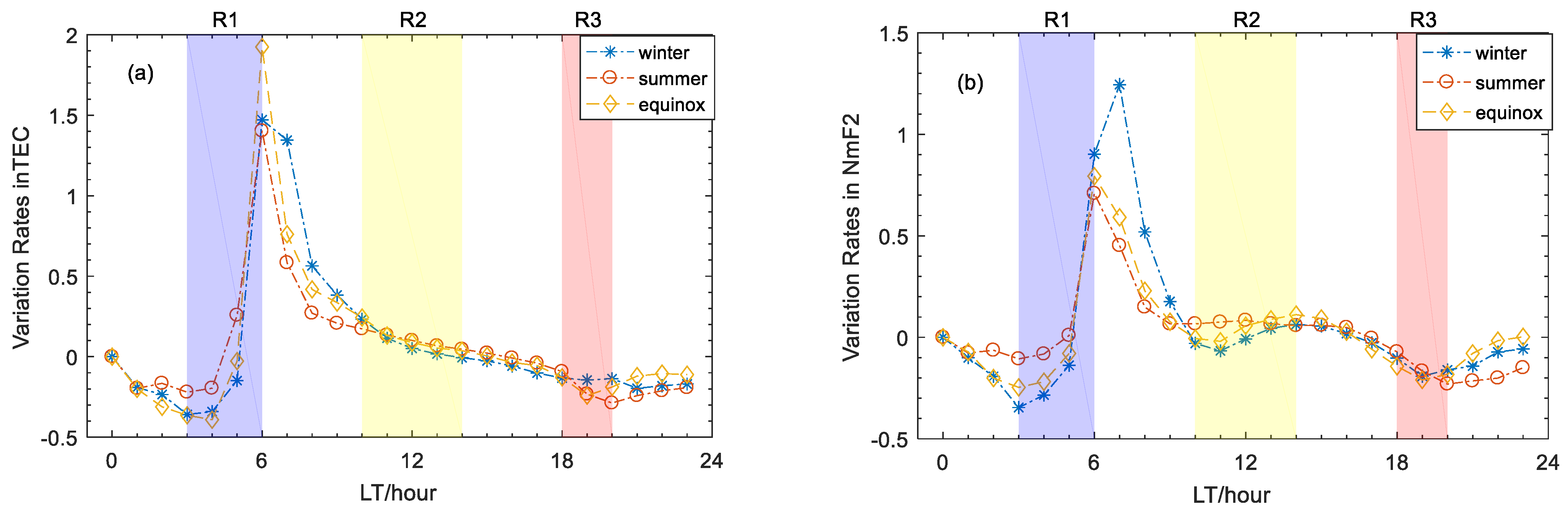
  • There is a post-sunset peak in τ observed during the winter and equinox, and it means that NmF2 is decreasing faster than TEC, which can be associated with the higher post-sunset TEC enhancement occurrence in equinox/winter, proving previous conclusions. In addition, the τ continues to decrease after post-midnight and the equinoctial one is smallest due to the largest nighttime NmF2 enhancement in equinox and the faster decrease in TEC in equinox than that in solstice.
  • The dependence of τ on the solar activity are different for daytime and nighttime: the daytime τ seems to increase with solar activity, as TEC is more sensitive to the solar activity than NmF2, whereas the nighttime one decreases with solar activity at night, and it should be due to the fact the H+-O+ transition height in the low solar activity is lower than that in the high solar activity at night.
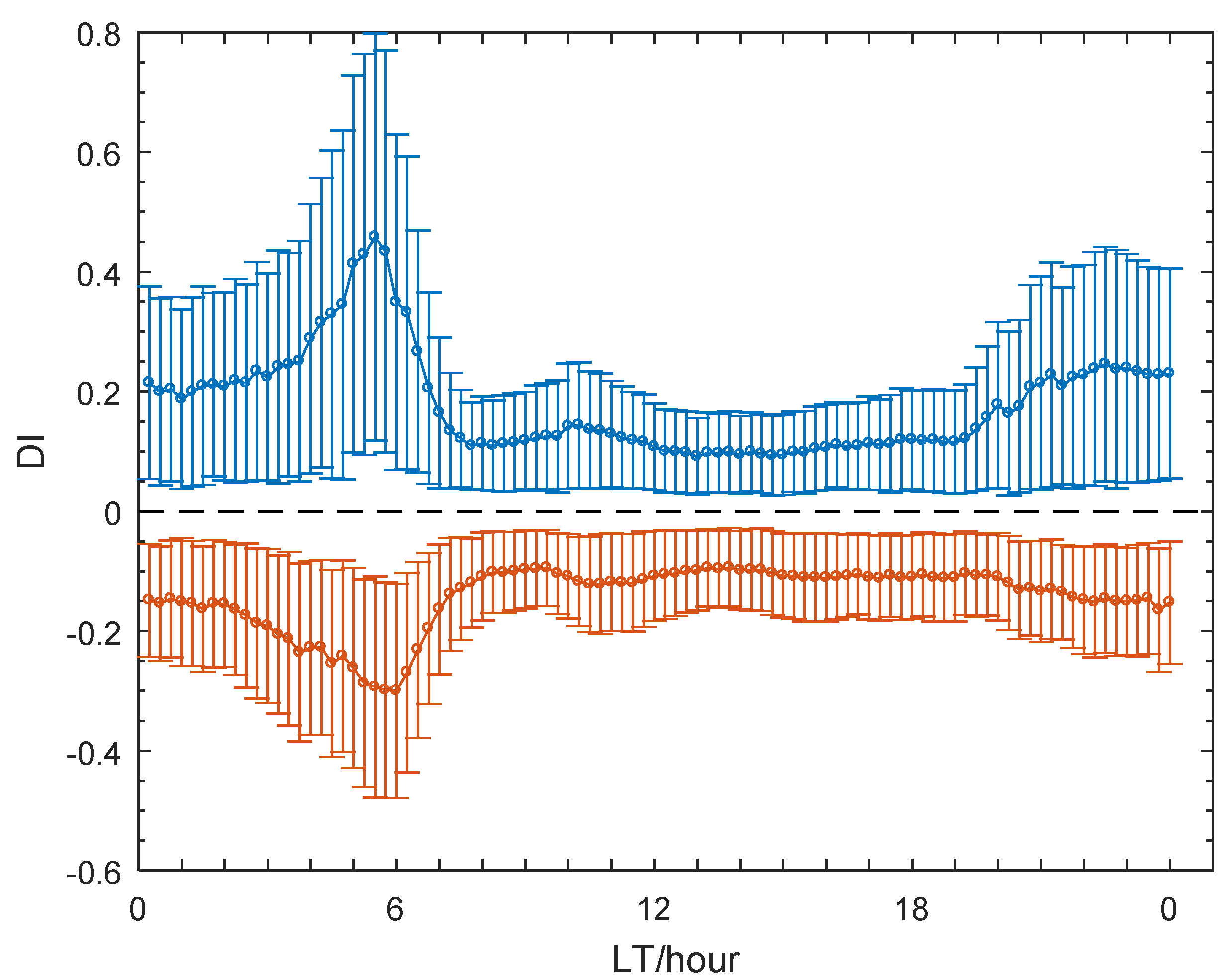
  • The τ has more variability during nighttime than daytime, during both the geomagnetically quiet and disturbed conditions, and the greatest variability of τ appeared at sunrise.
Moreover, we obtained some new results, which provide interesting insights into τ of this region:
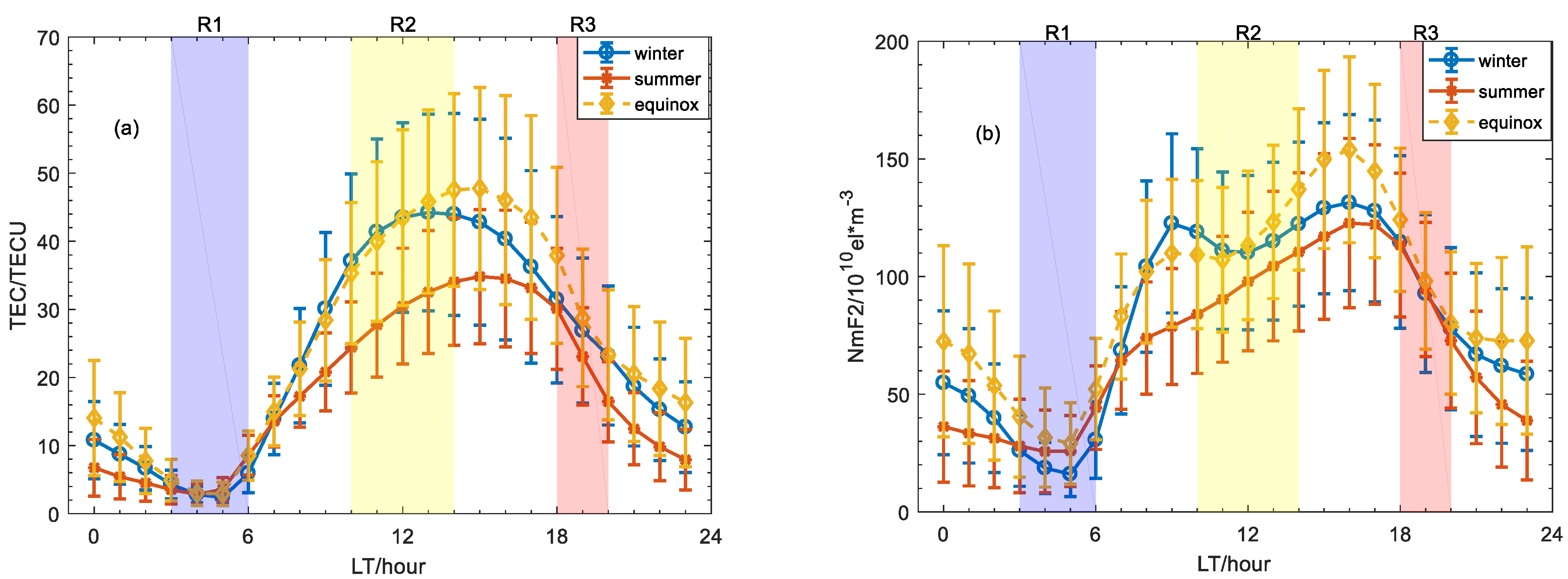
  • The τ at noon is larger in winter and equinox than in summer. It is probably due to the absence of NmF2 noontime bite-out in summer at this region.
  • There is no pre sunrise peak in τ and τ get low values during the pre-sunrise period at Guam. However, previous studies indicate that pre sunrise peak is a widely observed feature, from low to high latitude, and τ even reaches maximum at sunrise for specific seasons. The contradiction is probably due to Guam being located at equatorial latitude, as the low values in the pre sunrise period could also be seen at other longitudinal equatorial latitude station. In addition, longitudinal difference might also contribute to the difference.
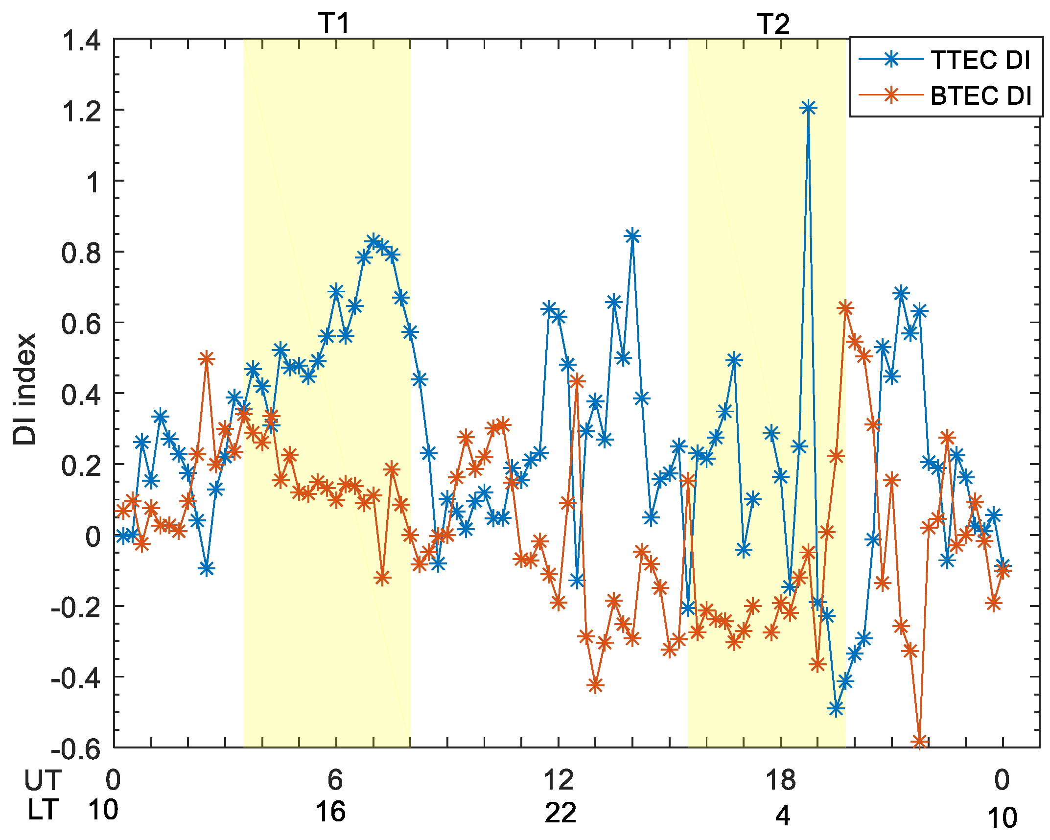
  • The geomagnetic storm seems to have a positive effect on the τ during most of the storm period in Guam, except at sunrise period, when the τ attains large variability, even at the geomagnetically quiet condition. This study also provides a new physical explanation for the observed effect of geomagnetic storm on τ in Guam. During the positive storms, the penetration electric field along with storm time equator-ward neutral wind tends to increase upward drift and uplift F region, causing the large increase in TEC accompanied by relatively small increase in NmF2. On the other hand, an enhanced equatorward wind tends to push more plasma, at low latitudes, into the topside ionosphere in the equatorial region, resulting in the TEC, which does not undergo severe depletion as NmF2 does during the negative storms. Therefore, the geomagnetic storm seems to enhance τ both during the positive and negative ionospheric storms.

Author Contributions

Conceptualization, Y.Z., Z.W. and T.X.; methodology, Z.D.; investigation, J.F. and Y.Z.; validation, Y.Z.; formal analysis, Y.Z. and W.X.; resources, M.O.; visualization, Z.D. and W.Z.; funding acquisition, M.O. All authors have read and agreed to the published version of the manuscript.

Funding

This work was supported by the National Key R&D Program of China(Grant No. 2018YFF0103700), Natural Science Basic Research Program of Shaanxi (Program No. 2020JQ-331).

Institutional Review Board Statement

Not applicable.

Informed Consent Statement

Not applicable.

Data Availability Statement

The use of ionosonde data provided by GIRO (Global Ionospheric Radio Observation) database (http://spase.info/SMWG/Observatory/GIRO accessed on 23 November 2021). The use of GPS data provided by UNAVCO database (University NAVSTAR Consortium) (http://www.unavco.org/ accessed on 23 November 2021).The use of Dst data provided by WDC (http://wdc.kugi.kyoto-u.ac.jp/ accessed on 23 November 2021). The use of F10.7 data provided by NOAA (ftp://ftp.swpc.noaa.gov/pub/indices/old_indices/ accessed on 23 November 2021).

Acknowledgments

We acknowledge the use of ionosonde data provided by GIRO (Global Ionospheric Radio Observation) database (http://umlcar.uml.edu/DIDbase accessed on 23 November 2021), GPS data provided by UNAVCO database (University NAVSTAR Consortium) (http://www.unavco.org/ accessed on 23 November 2021), Dst data provided by WDC (http://wdc.kugi.kyoto-u.ac.jp/ accessed on 23 November 2021) and F10.7 data provided by NOAA (ftp://ftp.swpc.noaa.gov/pub/indices/old_indices/ accessed on 23 November 2021).

Conflicts of Interest

The authors declare no conflict of interest.

References

  1. Breed, A.M.; Goodwin, G.L.; Vandenberg, A.-M.; Essex, E.A.; Lynn, K.J.W.; Silby, J.H. Ionospheric total electron content and ionospheric slab thickness determined in Australia. Radio Sci. 1997, 62, 1635–1643. [Google Scholar] [CrossRef]
  2. Wright, J.W. A model of the F-region above hmaxF2. J. Geophys. Res. 1960, 65, 185–191. [Google Scholar] [CrossRef]
  3. Titheridge, J.E. The ionospheric slab thickness of the mid-latitude ionosphere. Planet Space Sci. 1973, 21, 1775–1793. [Google Scholar] [CrossRef]
  4. Jakowski, N.; Putz, E.; Spalla, P. Ionospheric storm characteristics deduced from satellite radio beacon observations at three European stations. Ann. Geophys. 1990, 8, 343–352. [Google Scholar]
  5. Jakowski, N.; Mielich, J.; Hoque, M.M.; Danielides, M. Equivalent ionospheric slab thickness at the mid-latitude ionosphere during solar cycle 23. In Proceedings of the 38th COSPAR Scientific Assembly, Bremen, Germany, 18–25 July 2010. [Google Scholar]
  6. Jakowski, N.; Hoque, M.M.; Mielich, J.; Hall, C. Equivalent ionospheric slab thickness of the ionosphere over Europe as an indicator of long-term temperature changes in the thermosphere. J. Atmos. Terr. Phys. 2017, 163, 92–101. [Google Scholar]
  7. Huang, Z.; Yuan, H. Climatology of the ionospheric slab thickness along the longitude of 120° E in China and its adjacent region during the solar minimum years of 2007–2009. Ann. Geophys. 2015, 33, 1311–1319. [Google Scholar] [CrossRef]
  8. Maltseva, O.A.; Mozhaeva, N.S.; Nikitenko, T.V. Comparison of model and experimental ionospheric parameters at high latitudes. Adv. Space Res. 2013, 51, 599–609. [Google Scholar] [CrossRef]
  9. Maltseva, O.A.; Mozhaeva, N.S.; Nikitenko, T.V. Validation of the Neustrelitz Global Model according to the low latitude ionosphere. Adv. Space Res. 2014, 54, 463–472. [Google Scholar] [CrossRef]
  10. Maltseva, O.A.; Mozhaeva, N.S. The Use of the Total Electron Content Measured by Navigation Satellites to Estimate Ionospheric Conditions. Int. J. Nav. Obs. 2016, 2016, 7016208. [Google Scholar] [CrossRef]
  11. Froń, A.; Galkin, I.; Krankowski, A.; Bilitza, D.; Hernández-Pajares, M.; Reinisch, B.; Li, Z.; Kotulak, K.; Zakharenkova, I.; Cherniak, I.; et al. Towards Cooperative Global Mapping of the Ionosphere: Fusion Feasibility for IGS and IRI with Global Climate VTEC Maps. Remote Sens. 2020, 12, 3531. [Google Scholar] [CrossRef]
  12. Gerzen, T.; Jakowski, N.; Wilken, V.; Hoque, M.M. Reconstruction of F2 layer peak electron density based on operational vertical total electron content maps. Ann. Geophys. 2013, 31, 1241–1249. [Google Scholar] [CrossRef] [Green Version]
  13. Krankowski, A.; Shagimuratov, I.I.; Baran, L.W. Mapping of foF2 over Europe based on GPS-derived TEC data. Adv. Space Res. 2007, 39, 651–660. [Google Scholar] [CrossRef]
  14. Bhonsle, R.V.; Da Rosa, A.V.; Garriott, O.K. Measurement of Total Electron Content and the Equivalent ionospheric slab thickness of the Mid latitude Ionosphere. Radio Sci. 1965, 69, 929–937. [Google Scholar]
  15. Kersley, L.; Hajeb-Hosseinieh, H. Dependence of ionospheric slab thickness on geomagnetic activity. J. Atmos. Terr. Phys. 1976, 38, 1357–1360. [Google Scholar] [CrossRef]
  16. Jin, S.; Cho, J.-H.; Park, J.-U. Ionospheric slab thickness and its seasonal variations observed by GPS. J. Atmos. Sol. Terr. Phys. 2007, 69, 1864–1870. [Google Scholar] [CrossRef]
  17. Huang, Y.N. Some results of ionospheric slab thickness observations at Lunping. J. Geophys. Res. 1983, 88, 5517–5522. [Google Scholar] [CrossRef]
  18. Davies, K.; Liu, X.M. ionospheric slab thickness in middle and low latitudes. Radio Sci. 1991, 26, 997–1005. [Google Scholar] [CrossRef]
  19. Minakoshi, H.; Nishimuta, I. Ionospheric electron content and equivalent ionospheric slab thickness at lower mid-latitudes in the Japanese zon. In Proc. Beacon Satellite Symposium (IBSS); University of Wales: Wales, UK, 1994; Volume 144. [Google Scholar]
  20. Gulyaeva, T.L.; Jayachandran, B.; Krishnankutty, T.N. Latitudinal variation of slab thickness. Adv. Space Res. 2004, 33, 862–865. [Google Scholar] [CrossRef]
  21. Jayachandran, B.; Krishnankutty, T.; Gulyaeva, T. Climatology of ionospheric slab thickness. Ann. Geophys. 2004, 22, 25–33. [Google Scholar] [CrossRef] [Green Version]
  22. Pignalberi, A.; Nava, B.; Pietrella, M.; Cesaroni, C.; Pezzopane, M. Midlatitude climatology of the ionospheric equivalent slab thickness over two solar cycles. J. Geod. 2021, 95, 124. [Google Scholar] [CrossRef]
  23. Guo, P.; Xu, X.; Zhang, G.X. Analysis of the ionospheric equivalent ionospheric slab thickness based on ground-based GPS/TEC and GPS/COSMIC RO. J. Atmos. Sol. Terr. Phys. 2011, 73, 839–846. [Google Scholar] [CrossRef]
  24. Odeyemi, O.O.; Adeniyi, J.O.; Oladipo, O.A.; Olawepo, A.O.; Adimu, I.A.; Oyeyemi, E.O. Ionospheric slab thickness investigation on slab-thickness and B0 over an equatorial station in Africa and comparison with IRI model. J. Atmos. Sol. Terr. Phys. 2018, 179, 293–306. [Google Scholar] [CrossRef]
  25. Odeyemi, O.O.; Adeniyi, J.O.; Oyeyemi, E.O.; Panda, S.K.; Jamjareegulgarn, P.J.; Olugbon, B.; Oluwadare, E.J.; Akala, A.O.; Olawepo, A.J.; Adewale, A.A. Morphologies of ionospheric-equivalent slab thickness and scale height over equatorial latitude in Africa. Adv. Space Res. 2021, in press. [Google Scholar] [CrossRef]
  26. Huang, H.; Liu, L.; Chen, Y.; Le, H.; Wan, W. A global picture of ionospheric slab thickness derived from GIM TEC and COSMIC radio occultation observations. J. Geophys. Res. Space Phys. 2016, 121, 867–880. [Google Scholar] [CrossRef]
  27. Fox, M.W.; Mendillo, M.; Klobuchar, J.A. Ionospheric equivalent ionospheric slab thickness and its modeling applications. Radio Sci. 1991, 26, 429–438. [Google Scholar] [CrossRef]
  28. Spalla, P.; Ciraolo, L. TEC and foF2 comparison. Ann. Geophys. 1994, 37, 929–938. [Google Scholar] [CrossRef]
  29. Jakowski, N.; Hoque, M.M. Global equivalent ionospheric slab thickness model of the Earth’s ionosphere. J. Space Weather Space Clim. 2021, 11, 10. [Google Scholar] [CrossRef]
  30. Àlàgbé, G.A. Quiet- and storm-time correlation of F2-layer ionospheric slab thickness and B0 at an equatorial station. Int. J. Res. Rev. Appl. Sci. 2012, 13, 133–138. [Google Scholar]
  31. Duarte-Silva, M.H.; Muella, M.T.A.H.; Silva, L.C.C.; de Abreu, A.J.; Fagundes, P.R. Ionospheric slab thickness at the equatorial anomaly region after the deep solar minimum of cycle 23/24. Adv. Space Res. 2015, 56, 1961–1972. [Google Scholar] [CrossRef]
  32. Gulyaeva, T.; Stanislawska, I. Night-day imprints of ionospheric slab thickness during geomagnetic storm. J. Atmos. Sol. Terr. Phys. 2005, 67, 1307–1314. [Google Scholar] [CrossRef]
  33. Stankov, S.M.; Warnant, R. Ionospheric slab thickness—Analysis, modelling and monitoring. Adv. Space Res. 2009, 44, 1295–1303. [Google Scholar] [CrossRef]
  34. Uwamahoro, J.C.; Giday, N.M.; Habarulema, J.B.; Katamzi-Joseph, Z.T.; Seemala, G.K. Reconstruction of storm-time total electron content using ionospheric tomography and artificial neural networks: A comparative study over the African region. Radio Sci. 2018, 53, 1328–1345. [Google Scholar] [CrossRef]
  35. Ciraolo, L.; Azpilicueta, F.; Brunini, C.; Meza, A.; Radicella, S. Calibration errors on experimental slant total electron content (TEC) determined with GPS. J. Geodesy. 2007, 81, 111–120. [Google Scholar] [CrossRef]
  36. Abe, O.; Villamide, X.O.; Paparini, C.; Radicella, S.; Nava, B.; Rodríguez Bouza, M. Performance evaluation of gnss-tec ionospheric slab thicknessimation techniques at the grid point in middle and low latitudes during different geomagnetic conditions. J. Geodesy 2017, 91, 409–417. [Google Scholar] [CrossRef]
  37. Adewale, A.; Oyeyemi, E.; Adeniyi, J.; Adeloye, A.; Oladipo, O. Comparison of total electron content predicted using the IRI-2007 model with GPS observations over Lagos, Nigeria. Indian J. Radio Space Phys. 2011, 40, 21–25. [Google Scholar]
  38. Seemala, G.; Valladares, C. Statistics of total electron content depletions observed over the South American continent for the year 2008. Radio Sci. 2011, 46, RS5019. [Google Scholar] [CrossRef]
  39. Olwendo, O.; Baki, P.; Mito, C.; Doherty, P. Characterization of ionospheric GPS Total Electron content (GPS TEC) in low latitude zone over the Kenyan region during a very low solar activity phase. J. Atmos. Sol. Terr. Phys. 2012, 84, 52–61. [Google Scholar] [CrossRef]
  40. Akala, A.; Seemala, G.; Doherty, P.; Valladares, C.; Carrano, C.; Espinoza, J.; Oluyo, S. Comparison of equatorial GPS-TEC observations over an African station and an American station during the minimum and ascending phases of solar cycle 24. Ann. Geophys. 2013, 31, 2085–2096. [Google Scholar] [CrossRef] [Green Version]
  41. Matamba, T.M.; Habarulema, J.B.; McKinnell, L.-A. Statistical analysis of the ionospheric response during geomagnetic storm conditions over South Africa using ionosonde and GPS data. Space Weather. 2015, 13, 536–547. [Google Scholar] [CrossRef]
  42. Akala, A.O.; Adewusi, E.O. Quiet-time and storm-time variations of the African equatorial and low latitude ionosphere during 2009–2015. Adv. Space Res. 2020, 66, 1441–1459. [Google Scholar] [CrossRef]
  43. De Dieu Nibigira, J.; Sivavaraprasad, G.; Ratnam, D.V. Performance analysis of IRI-2016 model TEC predictions over Northern and Southern Hemispheric IGS stations during descending phase of solar cycle 24. Acta Geophys. 2021, 69, 1509–1527. [Google Scholar] [CrossRef]
  44. Reinisch, B.W.; Galkin, T.A. Global ionospheric radio observatory (GIRO). Earth Planets Space 2011, 63, 377–381. [Google Scholar] [CrossRef] [Green Version]
  45. England, S.L.; Immel, T.J.; Huba, J.D.; Hagan, M.E.; Maute, A.; DeMajistre, R. Modeling of multiple effects of atmospheric tides on the ionosphere: An examination of possible coupling mechanisms responsible for the longitudinal structure of the equatorial ionosphere. J. Geophys. Res. Space Res. 2010, 124, A05308. [Google Scholar] [CrossRef] [Green Version]
  46. Chen, Y.; Liu, L.; Le, H.; Wan, W.; Zhang, H. Equatorial ionization anomaly in the low-latitude topside ionosphere: Local time evolution and longitudinal difference. J. Geophys. Res. Space Res. 2016, 121, 7166–7182. [Google Scholar] [CrossRef]
  47. Lühr, H.; Häusler, K.; Stolle, C. Longitudinal variation of F region electron density and thermospheric zonal wind caused by atmospheric tides. Geophys. Res. Lett. 2007, 34, L16102. [Google Scholar] [CrossRef]
  48. Aggson, T.L.; Herrero, F.A.; Johnson, J.A.; Pfaff, R.F.; Laakso, H.; Maynard, N.C.; Moses, J.J. Satellite observations of zonal electric fields near sunrise in the equatorial ionosphere. J. Atmos. Sol. Terr. Phys. 1995, 57, 19–24. [Google Scholar] [CrossRef]
  49. Kelley, M.C.; Rodrigues, F.S.; Pfaff, R.F.; Klenzing, J. Observations of the generation of eastward equatorial electric fields near dawn. Ann. Geophys. 2014, 32, 1169–1175. [Google Scholar] [CrossRef] [Green Version]
  50. Zhang, R.; Liu, L.; Chen, Y.; Le, H. The dawn enhancement of the equatorial ionospheric vertical plasma drift. J. Geophy. Res: Space Phys. 2015, 120, 688–697. [Google Scholar] [CrossRef]
  51. Zhou, X.; Liu, H.-L.; Lu, X.; Zhang, R.; Maute, A.; Wu, H.; Yue, X.; Wan, W. Quiet-time day-to-day variability of equatorial vertical E × B drift from atmosphere perturbations at dawn. J. Geophys. Res. Space Phys. 2020, 124, e2020JA027824. [Google Scholar] [CrossRef]
  52. Balan, N.; Rao, P.B. Dependence of the ionospheric response on the local time of sudden commencement and the intensity of the geomagnetic storms. J. Atmos. Terr. Phys. 1990, 52, 269–275. [Google Scholar] [CrossRef]
  53. Kashcheyev, A.; Migoya-Orue, Y.; Amory-Mazaudier, C.; Fleury, R.; Nava, B.; Alazo-Cuartas, K.; Radicella, S.M. Multivariable comprehensive analysis of two great geomagnetic storms of 2015. J. Geophys. Res: Space Phys. 2018, 123, 5000–5018. [Google Scholar] [CrossRef]
  54. Buonsanto, M.J. Ionospheric storms—A review. Space Sci. Rev. 1999, 88, 563–601. [Google Scholar] [CrossRef]
  55. Mendillo, M. Storms in the ionosphere: Patterns and processes for total electron content. Rev. Geophys. 2006, 44, 335–360. [Google Scholar] [CrossRef]
  56. Immel, T.J.; Sagawa, S.L.; England, S.B.; Henderson, M.E.; Hagan, S.B.; Mende, H.U.; Frey, C.; Swenson, M.; Paxton, L.J. Control of equatorial ionospheric morphology by atmospheric tides. Geophys. Res. Lett. 2006, 33, L15108. [Google Scholar] [CrossRef]
  57. Rishbeth, H.; Mendillo, M. Patterns of F2-layer variability. J. Atmos. Sol. Terr. Phys. 2001, 63, 1661–1680. [Google Scholar] [CrossRef]
  58. Fang, T.-W.; Fuller-Rowell, T.; Yudin, V.; Matsuo, T.; Viereck, R. Quantifying the sources of ionosphere day-to-day variability. J. Geophys. Res. Space Phys. 2018, 123, 9682–9696. [Google Scholar] [CrossRef]
  59. Rajaram, G.; Rastogi, R.G. Equatorial Electron Densities—Seasonal and Solar Cycle Changes. J. Atmos. Terr. Phys. 1977, 39, 1175–1182. [Google Scholar] [CrossRef]
  60. Radicella, S.M.; Adeniyi, J.O. Equatorial ionospheric electron density below the F2 peak. Radio Sci. 1999, 34, 1153–1163. [Google Scholar] [CrossRef]
  61. Lee, C.C. Examination of the absence of noontime bite-out in equatorial total electron content. J. Geophys. Res. Space Res. 2012, 117, A09303. [Google Scholar] [CrossRef]
  62. Chen, Y.; Liu, L.; Le, H.; Zhang, H. Equatorial North-South Difference of Noontime Electron Density Bite-out in the F2-layer. J. Geophys. Res. Space Res. 2020, 125, e2020JA028124. [Google Scholar] [CrossRef]
  63. Su, Y.Z.; Bailey, G.J.; Balan, N. Night-time enhancements in TEC at equatorial anomaly latitudes. J. Atmos. Terr. Phys. 1993, 56, 1619–1628. [Google Scholar] [CrossRef]
  64. Agrawal, A.; Maski, K.; Vijay, S.K.; MaShra, S.D. An Analytical Study of Nighttime Enhancement in foF2 during 23rd& 24th Solar Cycle at Low Latitude Station. Int. J. Eng. Trends Tech. 2018, 61, 25–30. [Google Scholar]
  65. Fox, M.W.; Mendillo, M.; Spalla, P. The variation of ionospheric slab thickness during geomagnetic storms. In Proceedings of the International Beacon Satellite Symposium (IBSS), Tucuman, Argentina, 27–30 March 1990. [Google Scholar]
  66. Bhuyan, P.K.; Lakha, S.; Tyagi, T.R. Equivalent ionospheric slab thickness of the ionosphere over 26°N through the ascending half of a solar cycle. Ann. Geophys. 1986, 4, 131–136. [Google Scholar]
  67. Balan, N.; Shiokawa, K.; Otsuka, Y.; Kikuchi, T.; Vijaya Lekshmi, D.; Kawamura, S.; Yamamoto, M.; Bailey, G.J. A physical mechanism of positive ionospheric storms at low latitudes and midlatitudes. J. Geophys. Res. Space Phys. 2010, 115, A02304. [Google Scholar] [CrossRef]
  68. Lei, J.; Zhu, Q.; Wang, W.; Burns, A.G.; Zhao, B.; Luan, X.; Zhong, J.; Dou, X. Response of the topside and bottomside ionosphere at low and middle latitudes to the October 2003 superstorms. J. Geophys. Res. Space Phys. 2015, 120, 6974–6986. [Google Scholar] [CrossRef]
  69. Lei, J.; Zhong, J.; Mao, T.; Hu, L.; Yu, T.; Luan, X.; Dou, X.; Sutton, E.; Yue, X.; Lin, J.; et al. Contrasting behavior of the F2 peak and the topside ionosphere in response to the 2 October 2013 geomagnetic storm. J. Geophys. Res. Space Phys. 2016, 121, 10549–10563. [Google Scholar] [CrossRef]
Figure 1. F10.7 variations during the years 2012–2017.
Remotesensing 13 05175 g001
Figure 2. An example for the calculation of DI index during the period 6–8 June 2013.
Remotesensing 13 05175 g002
Figure 3. Map of mean (a) and standard deviation (b) of equivalent slab thickness (τ) under geomagnetically quiet condition, according to January–December and 0LT–23LT division in 2012–2017.
Remotesensing 13 05175 g003
Figure 4. Map of mean and standard deviation of equivalent slab thickness (τ) under geomagnetically quiet condition. (a) Mean of τ in high solar activity year 2014; (b) Mean of τ in low solar activity year 2016; (c) Standard deviation of τ in high solar activity year 2014; (d) Standard deviation of τ in low solar activity year 2016.
Remotesensing 13 05175 g004aRemotesensing 13 05175 g004b
Figure 5. Diurnal variations of mean and standard deviation of equivalent slab thickness (τ) in winter, summer, and equinox at geomagnetically quiet condition.
Remotesensing 13 05175 g005
Figure 6. Diurnal variation of the mean and standard deviation (STD) of DI index at geomagnetically quiet conditions.
Remotesensing 13 05175 g006
Figure 7. Same as Figure 6 but for geomagnetic storm periods.
Remotesensing 13 05175 g007
Figure 8. (a) Comparison of diurnal DI index for geomagnetically quiet condition and geomagnetic storm condition (b) The minus between the DI index during geomagnetic storm periods and DI index at geomagnetically quiet time, according to the sign of DI.
Remotesensing 13 05175 g008
Figure 9. (a) Diurnal variations of mean and standard deviation of total electron content (TEC) in Guam during winter, summer, and equinox, respectively. (b) Diurnal variations of mean and standard deviation of F2-layer peak electron density (NmF2) in Guam during winter, summer, and equinox, respectively.
Remotesensing 13 05175 g009
Figure 10. (a) Variation rates in TEC for winter, summer, and equinox, respectively. (b) Variation rates in NmF2 for winter, summer, and equinox, respectively.
Remotesensing 13 05175 g010
Figure 11. The geophysical conditions during 1–2 June 2013.
Remotesensing 13 05175 g011
Figure 12. (a) The DI index of TEC and NmF2 on 1 June 2013. (b) The DI index of τ on 1 June 2013.
Remotesensing 13 05175 g012
Figure 13. The DI index of TTEC and BTEC on 1 June 2013.
Remotesensing 13 05175 g013
Table 1. Mean daytime (08:00–16:00LT) and night-time (20:00–04:00LT) values of ionospheric equivalent slab thickness (τ) for magnetically quiet days during the high solar activity year 2014 and the low solar activity year 2016.
YearSeasonsMean Daytime Values of τ (km) Mean Nighttime Values of τ (km)
2014Winter388.9232.1
Summer303.9188.9
Equinox364.6250.7
2016Winter299.3255.5
Summer288.6238.5
Equinox301.2268.4
Publisher’s Note: MDPI stays neutral with regard to jurisdictional claims in published maps and institutional affiliations.

