
Mapping Large-Scale Forest Disturbance Types with Multi-Temporal CNN Framework
by
 ,
,
Xi Chen
1,2,3,†, 
Wenzhi Zhao
1,2,†,
Jiage Chen
4,*,
Yang Qu
5,
Dinghui Wu
3,6 and
Xuehong Chen
1,2 1
State Key Laboratory of Remote Sensing Science, Faculty of Geographical Science, Institute of Remote Sensing Science and Engineering, Beijing Normal University, Beijing 100875, China
2
Beijing Engineering Research Center for Global Land Remote Sensing Products, Faculty of Geographical Science, Institute of Remote Sensing Science and Engineering, Beijing Normal University, Beijing 100875, China
3
State Key Laboratory of Information Engineering in Surveying, Mapping and Remote Sensing, Wuhan University, Wuhan 430079, China
4
National Geomatics Center of China, Beijing 100830, China
5
School of Remote Sensing and Information Engineering, Wuhan University, Wuhan 430079, China
6
School of Surveying and Geo-Informatics, Shandong Jianzhu University, Jinan 250101, China
*
Author to whom correspondence should be addressed.
†
Both authors contributed equally to this work and should be considered co-first authors.
Remote Sens. 2021, 13(24), 5177; https://0-doi-org.brum.beds.ac.uk/10.3390/rs13245177
Submission received: 24 October 2021
/
Revised: 10 December 2021
/
Accepted: 16 December 2021
/
Published: 20 December 2021
(This article belongs to the Special Issue Remote Sensing and Geospatial Approaches for Studying the Environment Affected by Human Activities)
Abstract
:Forests play a vital role in combating gradual developmental deficiencies and balancing regional ecosystems, yet they are constantly disturbed by man-made or natural events. Therefore, developing a timely and accurate forest disturbance detection strategy is urgently needed. The accuracy of traditional detection algorithms depends on the selection of thresholds or the formulation of complete rules, which inevitably reduces the accuracy and automation level of detection. In this paper, we propose a new multitemporal convolutional network framework (MT-CNN). It is an integrated method that can realize long-term, large-scale forest interference detection and distinguish the types (forest fire and harvest/deforestation) of disturbances without human intervention. Firstly, it uses the sliding window technique to calculate an adaptive threshold to identify potential interference points, and then a multitemporal CNN network is designed to render the disturbance types with various disturbance duration periods. To illustrate the detection accuracy of MT-CNN, we conducted experiments in a large-scale forest area (about 990 ) on the west coast of the United States (including northwest California and west Oregon) with long time-series Landsat data from 1986 to 2020. Based on the manually annotated labels, the evaluation results show that the overall accuracies of disturbance point detection and disturbance type recognition reach . Also, this method is able to detect multiple disturbances that continuously occurred in the same pixel. Moreover, we found that forest disturbances that caused forest fire repeatedly appear without a significant coupling effect with annual temporal and precipitation variations. Potentially, our method is able to provide large-scale forest disturbance mapping with detailed disturbance information to support forest inventory management and sustainable development.
1. Introduction
Amid radical global environmental degradation, forests with worldwide coverage play a vital role in promoting human sustainable development. In terms of balancing the regional ecology system, forests are also able to regulate regional climate as well as carbon and water cycles [1,2,3]. Nevertheless, most existing forest ecosystems are continuously disturbed by natural and human-made events, such as fires, pests, and deforestation, which seriously harms the local ecosystem and wildlife population structure [4,5]. It is urgently needed to develop appropriate land management strategies using accurate forest disturbance maps through long time-series archived remote sensing data. Conventional forest ecology methods often require intensive field investigation and consume abundant resources, but it is difficult to achieve satisfactory forest disturbance detection results on large-scales [6]. Therefore, developing a timely and accurate forest disturbance detection strategy is urgently needed.
Earth observation satellites are designed to acquire land surface images constantly with a long-time span and large-scale coverage, which was long considered an ideal solution to comprehensively investigate forest disturbances [7]. Since the free opening of the U.S. Geological Service (USGS) Landsat data archive in 2008, it provides large amounts of medium-resolution optical imagery dating back to 1972 [8,9]. Densely formed time-series remote sensing data can dynamically identify the annual forest disturbance and characterize the magnitude and duration of the disturbance [10]. Aiming to detect forest disturbances, intensive studies emerged for the sake of abundant time-series remote sensing imagery, which significantly promoted the relevant research. However, direct identifying forest disturbances almost impossible due to substantial random noises produced by atmospheric effects, the sunlit angle variation, and sensor degradation. Therefore, the challenge of detecting large-scale forest disturbance is how to identify disturbance signals from a large amount of noisy background.
The conventional forest disturbance identification strategy in remote sensing society is to use the vegetation index (such as the normalized difference vegetation index (NDVI) and normalized burn ratio (NBR)) quantifying the degree of changes compared to the standard unchanged targets’ profile [11,12]. For instance, The VCT algorithm designed the integrated forest Z-score (IFZ) index to represent the possibility of forest pixels and developed a set of rules to determine forest disturbances [13,14]. Such methods usually require predefined standard time-series curves before iterative comparison for disturbance determination [15]. However, due to the influence of random noise, even the same type of forest may present great differences in time-series vegetation indices. For this reason, the conventional difference measurements (such as Euclidean distance or Mahalanobis distance) are often failed to calculate inconsistency between the target time-series and standard ones. To alleviate the above problem, Landtrendr method uses straight-line segments to fit the representative features of the Landsat time-series signals. It simplifies the complex time-series into straight-line feature comparison, which reduces random noise interference to a certain degree [16]. Following a different strategy, dynamic time warping (DTW) constructs the optimal nonlinear alignment between two time-series, which can overcome the time deviation effectively [17,18]. Meanwhile, The Breaks For Additive Season and Trend Monitor (BFAST) algorithm decomposes Landsat time-series pixels into the trend, season, and noise components and determines forest disturbance by continually comparing the disturbed time-series profile with the historically stable forest profile [19,20]. Moreover, the CCDC algorithm constructs a physical prediction model and detects disturbance points by comparing the prediction with the real-time series. The model can adapt to noise when given enough coefficients [21,22]. Currently, CCDC was integrated on the Google Earth Engine (GEE) platform and plays as the benchmark for forest disturbance validation [23,24,25]. Still, these methods are built on prior knowledge or assumptions, and the process of disturbances detection must go through a series of iterative curve filtering or parameter optimization. Therefore, the accuracy of detection solely depends on the selection of threshold parameters and complete rule formulation, which inevitably deteriorate the detection accuracies and automation levels [26]. Thus, it is necessary to develop self-adaptative and autonomous detection methods for the improvement of forest disturbance identification.
Deep learning strategies, which extract high-level features through hierarchy structures, were widely used in time-series information extraction tasks [27]. Compared with traditional methods based on hand-crafted rules or thresholds, the high-level features learned by deep learning are more representative [28]. At present, deep networks such as CNN and LSTM were intensively used for large-scale agricultural and forestry monitoring, such as forest coverage prediction and crop phenology detection [29,30]. Specifically, Kong et al. (2018) [31] proposed a strategy to learn stable forest time-series with LSTM network from historical data, which then allows for the forest disturbance detection to be identified by comparing the predicted data and real data. Ban et al. (2020) [32] achieved near real-time localization of forest fires with the assistance of a multilayer CNN framework. Thus, the mentioned studies are designated to detect forest disturbances given the abnormality. Still, the types of disturbances (i.e., fire, deforestation) is often needed before a reasonable decision can be made for forest protection.
For a typical forest disturbance time-series, it can be decomposed into two subprofiles that are the disturbance process (shown as a rapid decline in the values of vegetation index) and a duration process (shown as a slow recovery of the vegetation values), respectively [33]. For example, after a forest fire event, the ecological forest infrastructure is fully destroyed, and it will take 10 years or more to restore to the original level, while for most deforestations, it can be quickly restored within few years (i.e., 3–5) [12,34,35]. But, most of the existing forest disturbance detection methods focus on the fixed-scale for disturbance process recognition and neglecting the recovery process measurement. Therefore, the relationship between disturbance types and their scale-variate duration process is often overlooked [36]. Moreover, different disturbances may constantly occur through a specific temporal range. How to iteratively detect forest disturbances also remains unexploited.
To solve the above problems, we propose a multitemporal convolutional network framework (MT-CNN) to recognize different types of forest disturbances. Specifically, we first detect potential forest disturbance points through a set of sliding windows techniques, which inevitably may contain a certain degree of noise. After that, the rough detection results are further being refined with a well-trained multitemporal CNN network. In addition, during the process of refinement, the disturbance types of the forest also to be determined. The main contributions of this paper are:
- (1)
- The sliding window scheme is being integrated with multiscale temporal CNN for forest disturbance type recognition with various duration periods.
- (2)
- The proposed MT-CNN can simultaneously achieve long-term and large-scale multiple forest disturbance detection without human intervention.
- (3)
- The prediction accuracy of forest disturbances is above on the USA west coast region with the past 35 years of Landsat time-series data.
The remainder of this paper is organized as follows: the research data and the details of the MT-CNN method are described in Section 2, and Section 3, respectively. Section 4 introduces the experiment of forest disturbance type detection and shows the experimental results. Discussion and conclusion are presented in Section 5 and Section 6, respectively.
2. Study Area and Data Preparation
2.1. Study Area
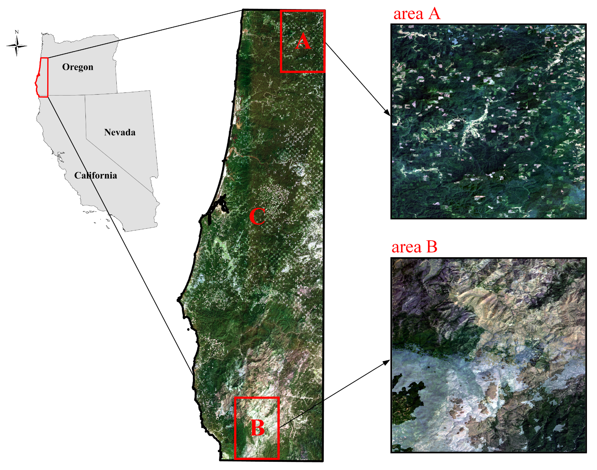
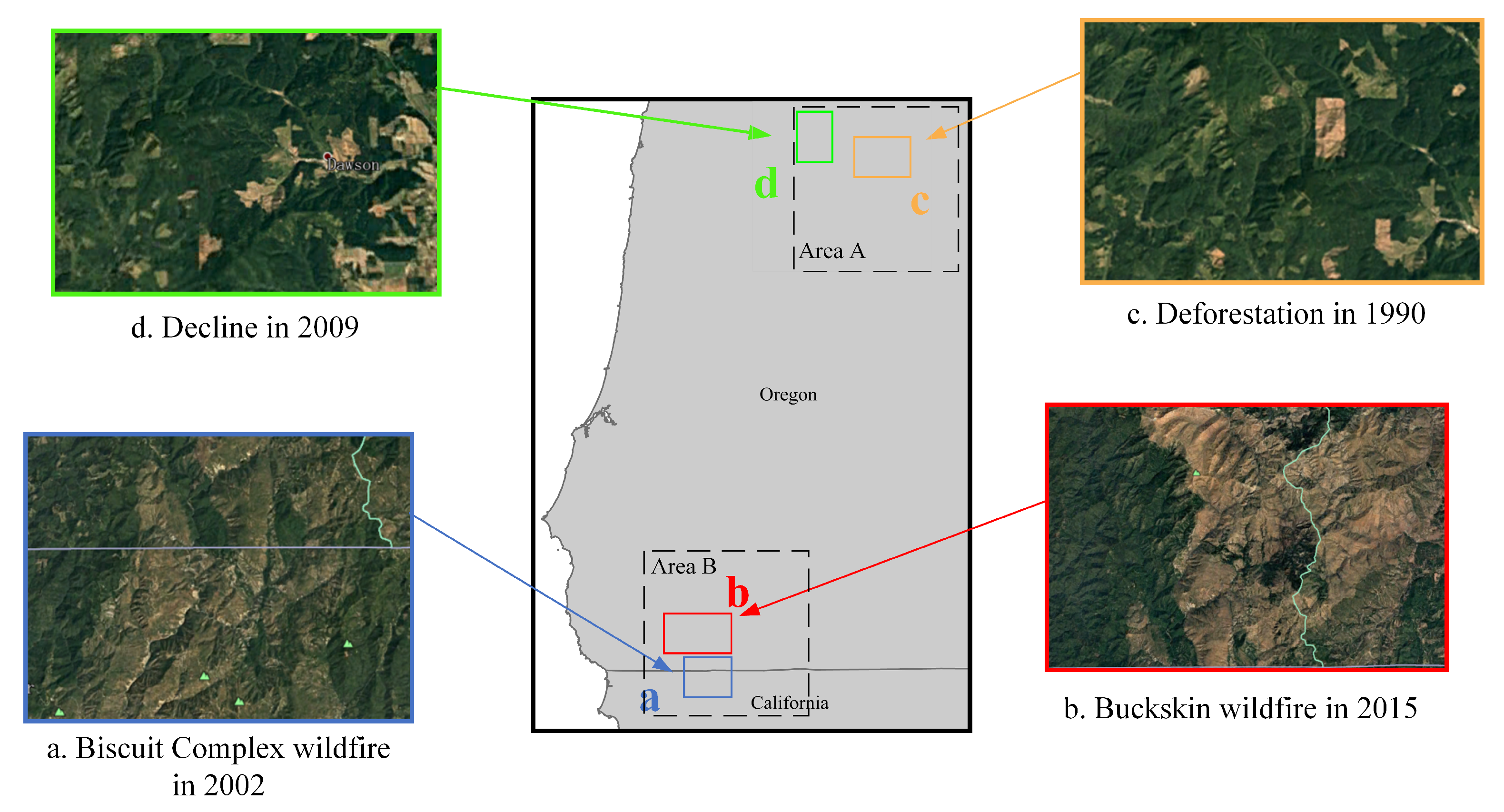
To fully demonstrate the performance of our proposed forest disturbance detection method, we conducted tests on a large-scale area at the west coast of USA. As shown in Figure 1), it is mainly located in northwestern California and western Oregon. The region mainly has a Mediterranean climate, with dry summers and rainy winters. Due to its unique geographical location, the region has a variety of forest types. Among them, the coastal area is mainly wet temperate rain forest, and the inland area has a large area of coniferous forest. Affected by the vast forest area and human activities, forest fires and anthropogenic deforestation constantly occurred.
2.2. Time-Series Data Acquisitions
2.2.1. Landsat Data
We constructed long time-series data from 1986 to 2020 for the study area, mainly consisting of annual composite images of Landsat in June, July, and August for each year. Among them, Landsat5 TM and Landsat8 OLI are the main data sources, while Landsat7 ETM+ is the auxiliary data to make up for the lack of data observation. To reduce the influence of clouds and cloud shadows, we do cloud masking for each image, and use the median of all available images each year as the annual composite pixel value. For forest disturbance detection, deforestation is manifested by the decrease of near-infrared () reflectance and forest fire has an obviously increase in short-wave infrared() reflectance [37,38]. Therefore, we preprocessed long time-series data to normalized burn ratio (), as it can effectively distinguish different types of forest disturbances such as forest fire and deforestation. The is formulated as .
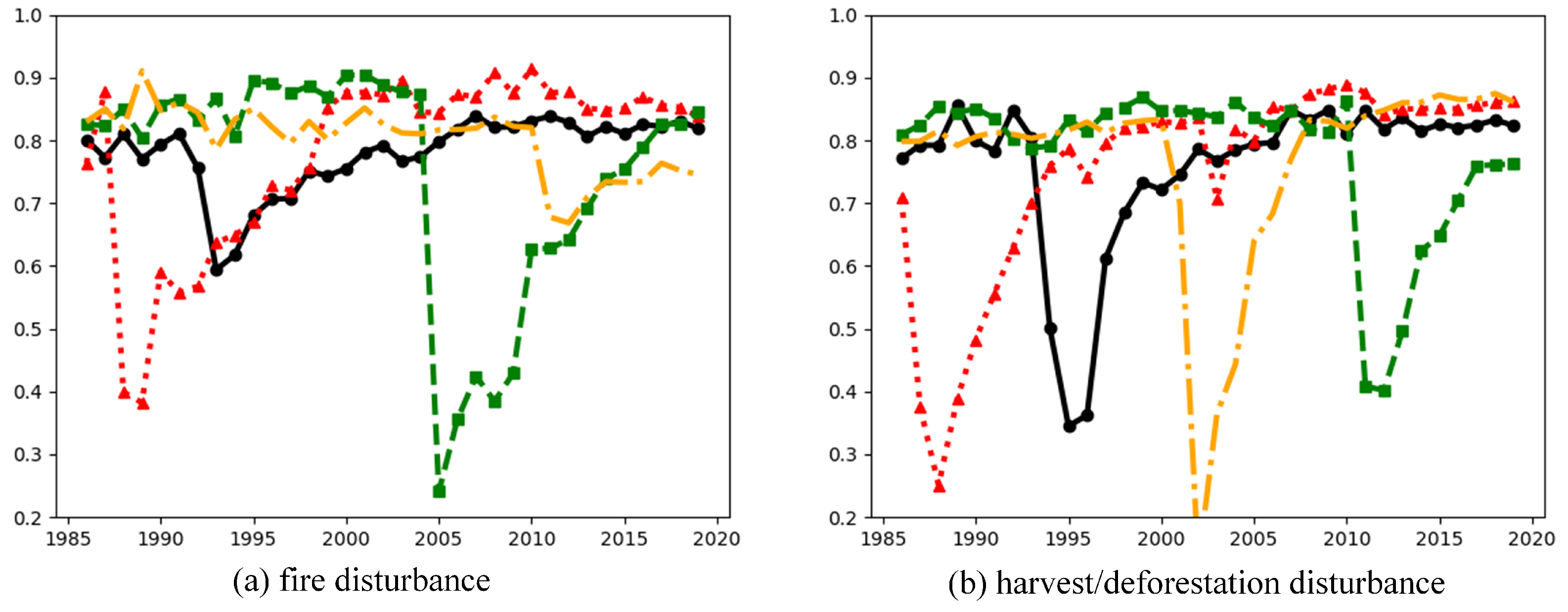
We drew some typical NBR curves in this area. As shown in Figure 2, wildfires and deforestation showed different characteristics in NBR time-series curves. For example, harvest/deforestation activities are usually only lasting for a short period, while a quick recovery can be observed. Differently, the forest fires usually with a long recovery period compared to human intervened deforestation.
Moreover, Since the long time-series data was constructed between three different sensors, TM and ETM+ were harmonized into OLI processing to maintain consistency [39]. All of the above processes are done on the GEE platform.
2.2.2. Disturbance Reference Data
We learned that in 2002, 2018, and 2020, several catastrophic wildfires occurred in Medford and Eugene in southern Oregon through related articles and fire monitoring websites (see area B in Figure 1). Meanwhile, the ever-increasing demand for the wood industry also caused the constant decline in forest inventory.We found a large number of harvest/deforestation areas from google earth platform (see area A in Figure 1). Therefore, we refer to two types of disturbances, that are harvest/deforestation and forest fires, as our forest disturbance detection objectives [40].
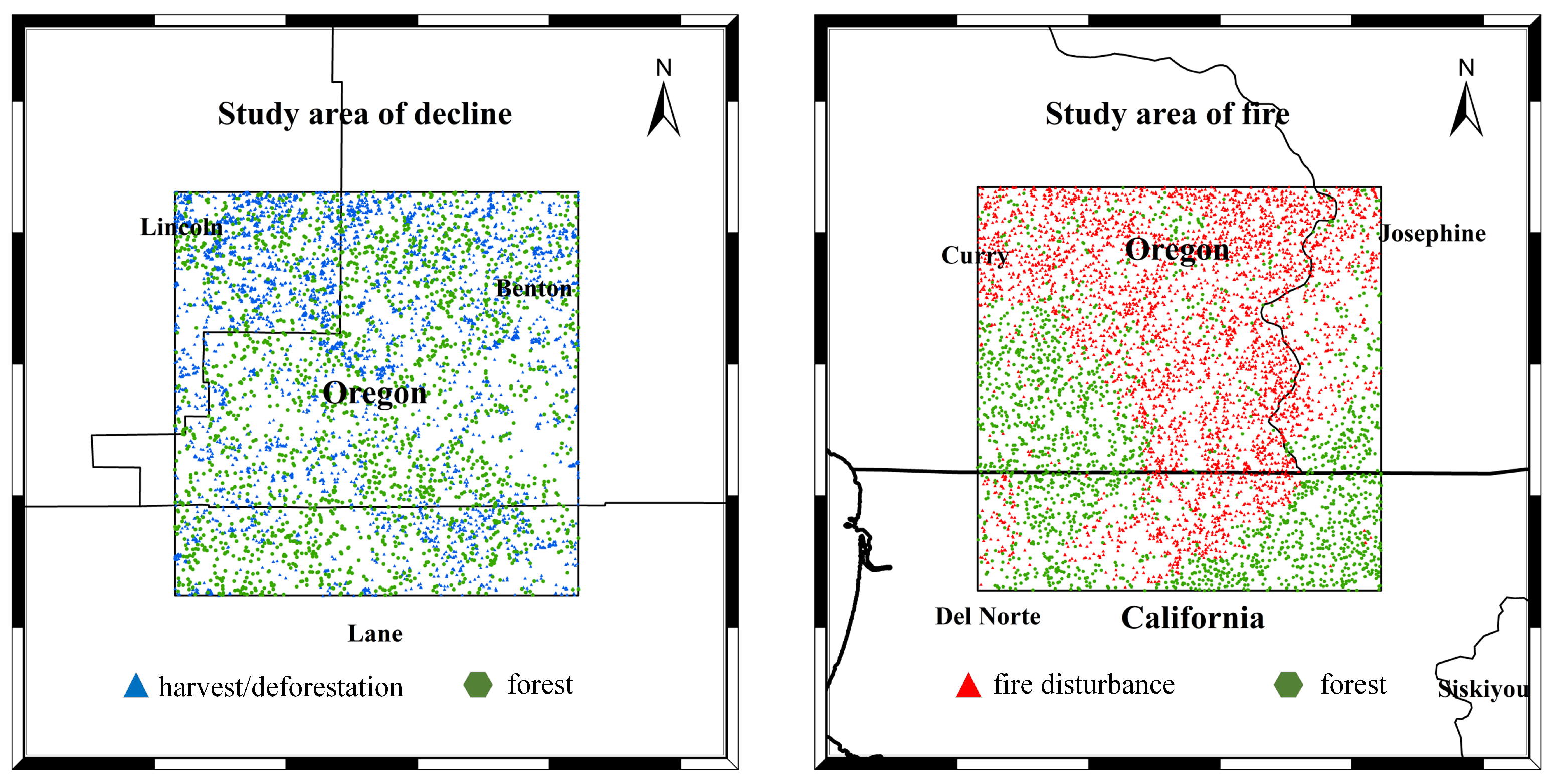
To validate the forest disturbance results by the proposed MT-CNN method, we obtained the high-precision forest disturbance samples by interactively combining the forest disturbance events and TimeSync interpretation tool [41]. We first convert the Landsat time series data into the standard format required by Timesync, and then visually distinguished fire and harvest/deforestation samples from nonchange ones combined with spatial information and NBR index.To ensure the uniform distribution of the samples, we randomly select a certain number of samples in area A and area B. In the end, we get 6000 samples in area A and area B, respectively (12,000 in total), of which 2000 stable forest samples were in each of the two regions, as shown in Figure 3.
3. Methodology
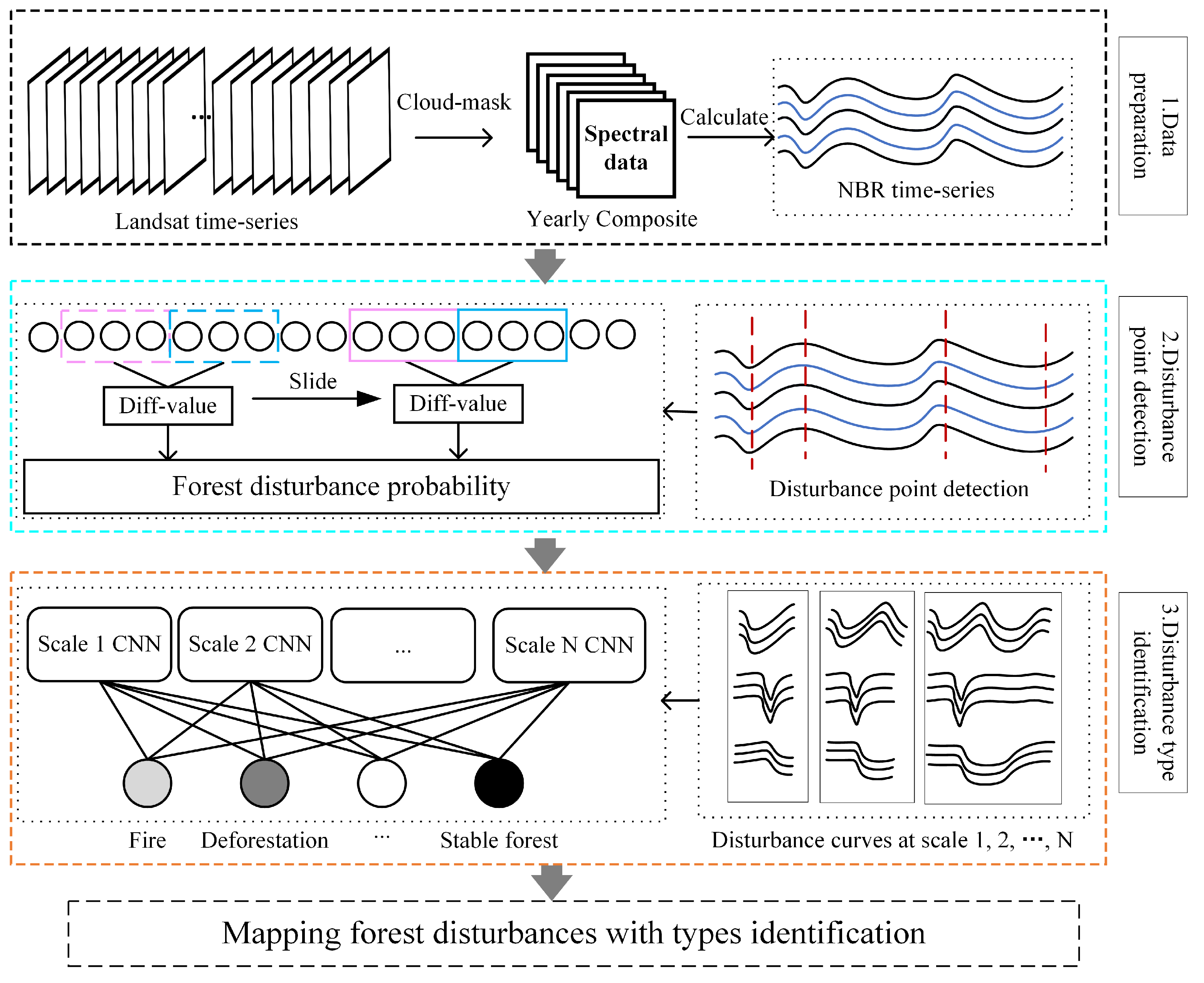
The proposed MT-CNN mainly consists of three modular units, that is, the data preparation module, the time-series breakpoint detection module, and the multiscale CNN disturbance type identification module. Specifically, we first construct the Landsat time-series stack and compute the NBR index to amplify forest disturbance signals. Then, a sliding window technique is applied to filter time-series signals which aim to detect possible breakpoints for forest disturbances. In this process, the thresholds for potential forest disturbances are automatically calculated by a self-adaptive scheme without human intervention. As a result, both real and pseudo disturbances may be detected. Finally, the rough detection results are input into the multitemporal CNN model to determine the type of forest disturbance and eliminate false detections. Based on the two-step detection process, various forest disturbances and their types can be determined through long time series data. The flowchart of the proposed MT-CNN method is shown in Figure 4.
3.1. Disturbance Point Detection
For most forest disturbance scenarios, the disturbance point is defined as the timing of a sudden decrease in the NBR value. Therefore, the sharp decline of NBR detection is the key to determine the forest disturbance time. For this purpose, we use a self-adaptive sliding window strategy to achieve disturbance point detection. For a given time series , the corresponding value is denoted by . We use two sliding windows side by side along with the time series to calculate the index difference between windows for disturbance points detection. Suppose that represents the time interval that in range of with window size b, . To catch the overall trend information, we compute the 2-norm for each window to represent the statistical characteristics of the signal. The discrepancy measurement for each sliding window can be expressed as:
where represents the L2-norm of the given time-series signals. We predict the disturbance point by the self-adaptive dynamic threshold technique. Specifically, the possible disturbance points are automatically evaluated by a quartile statistical method. Firstly, we arrange the window trend signals obtained in the previous step from small to large and get the values and of their 1/4 and 3/4 positions according to the linear rule. Then the interquartile range (r) of the signal can be expressed as:
We take the self-adaptive factor on the quarterback difference as the abnormal threshold, then the range of normal data can be expressed as:
Since, the forest disturbance scene usually shows that the value suddenly drops, so we only take the lower bound of this range. The range formula of the disturbance point is .
3.2. MT-CNN for Disturbance Type Recognition
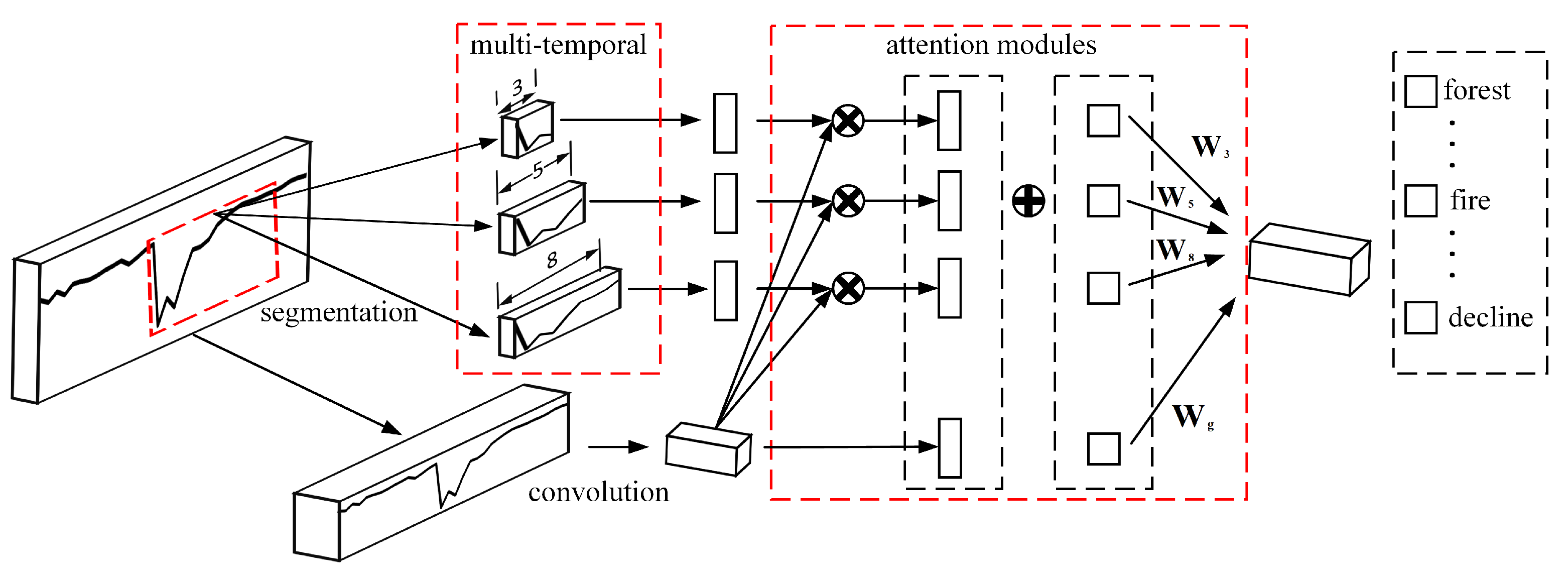
The flowchart of our proposed multitemporal CNN framework is shown in Figure 5. To achieve the purpose of disturbance type recognition, we developed a multitemporal scheme to extract rapid decline and recovery process time-series fragments through forest regions at different scales. Meanwhile, the convolutional neural network is applied to automatically detect the disturbance types of the extracted time-series fragments. Specifically, we extracted the multitemporal fragments with various lengths begin with the disturbance points detected in Section 3.1. For the part with insufficient length, the last point of the time series is replicated to the extent of desired lengths. For the extracted time-series fragments at different scales , we use multitemporal convolutional neural networks to extract cross-scale disturbance features.
where represents the time-series fragments at different temporal scales, and represent learnable weights and bias for the multitemporal CNN framework. With increasing length of time series fragments, the number of layers n of convolutional layer and subsampling layer can be automatically adjusted. To accurately measure the general disturbance characteristics for each temporal scale, we proposed an overall multitemporal attention mechanism to the CNN framework. This process aims to learn the relative features of each time-series fragment relative to the whole time-series, so as to increase its discrimination. For the attention mechanism, we have
where represents the whole time-series, represents the attention indicator of the deep features extracted from multitemporal CNN for the specific scale l. M represents the dimension of extracted deep features. During the training process, the multitemporal attention term gradually learns the relationship between the disturbance types and multitemporal deep features. Since the weights of the cross-scale network are determined, the probability of disturbance type for each scale also can be deduced. This process can be represented as:
Finally, the output probabilities of cross-scale CNNs are connected through the fully connected layer, allowing the model to be trained by optimizing a multiscale loss function. In this process, we get the final prediction for each sample across all-scale time-series fragments on forest disturbance types. Specifically, to strengthen the cross-scale ability of MT-CNN, we integrated all probabilities on various time-series fragments to get the final prediction. Therefore, the final forest disturbance prediction can be formulated as
where C describes the number of forest disturbance types. Thus, in this process, CNN predictions at different scales are integrated into the final predict disturbance types. In addition, this modular is also able to correct the false detection in Section 3.1.
4. Experiments and Results
In this section, we apply the MT-CNN algorithm to two areas on the west coast of the United States that contain specific types of disturbances for qualitative evaluation (area A and area B in Figure 1). To illustrate the capability of the proposed method, we randomly select of the manually labeled samples as the training set and the rest as the test ones. Accuracy metrics such as users’ accuracy, producers’ accuracy, confusion matrix, and precision rate are used to evaluate the detection accuracy of forest disturbance. In addition, we also analyzed the evaluation results into three levels: disturbance type, disturbance time, and the number of occurrences for each time-series signal. In the following sections, we conduct a qualitative and quantitative evaluation of the disturbance detection in the study area.
4.1. Large-Scale Forest Disturbance Mapping
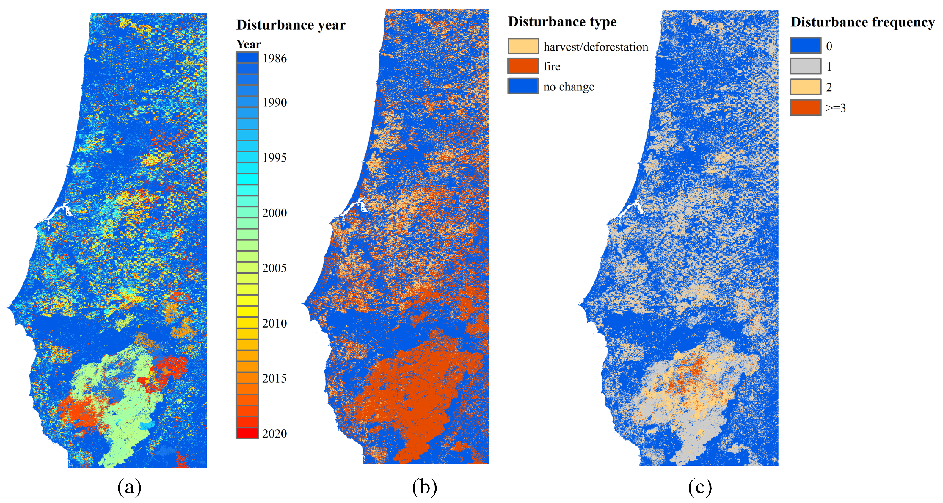
To demonstrate the robustness of the proposed method, we used the MT-CNN method to predict forest disturbances over a large-scale area of the USA west coast. With the proposed modular, the forest disturbances with different types are accurately identified. The forest disturbance results are illustrated in Figure 6.
Firstly, for the disturbance point detection from Figure 6a, we can conclude that most disturbances occurred in 2002 and 2019 as there were two devastating wildfires broke out. From 1986 to 2020, the yearly area of forest disturbances has witnessed a continuous increase, especially since the year 2001. From a regional perspective, small forest disturbances can be observed in the north region of the study area, while the large disturbance areas are mainly located in the south region. Before the year 2000, forest disturbances are sparsely distributed in the study area and the majority of them are near the fringe area of the deep forest. While, after the year 2000, large-scale forest disturbances are frequently observed, especially for the mountainous and deep forest regions.
Secondly, for the disturbance type identification from Figure 6b, the majority disturbance type of our study area is fire instead of harvest/deforestation. In general, there are 10,894,868 pixels of detected fire disturbances and 4,361,100 pixels of harvest/deforestation disturbances. Similarly, to the disturbance year, a large area of fire disturbances occurred in the south region of the study area, while the north part of the study area is mainly with harvest/deforestation. With the spatial integration of disturbance point and disturbance type, we can conclude that sparsely distributed forest disturbances in the north region are mainly harvest/deforestation. The reason for this phenomenon probably is human intervened urbanization. While for the south region of the study area, forest fire is the prominent impact factor for forest sustainability.
Thirdly, from the perspective of disturbance frequency, we can identify the most unstable area that suffers from continuous disturbances, as shown in Figure 6c. For the detected forest disturbances, there is (9,704,841) pixels had occurred one-time disturbance over the last 3 decades. Another detected pixels had encountered two-time disturbances, such as fire-fire or harvest/deforestation-fire. Combining the mapping results of disturbance point and type, we can deduce that high-frequency forest disturbance areas are located in the deep forest region. Meanwhile, the disturbance type is mainly forest fire with the first appearance in the year 1990. Over the last three decades, this region is continuously suffered from forest fire disturbance until 2020.
In general, the study area has mainly two types of forest disturbances, i.e., fire and harvest/deforestation. Most disturbances that occurred in this region is caused by wildfire outbreak. Compared to that of the existing forest disturbance detection algorithm, the MT-CNN is able to detect repeatedly occurred disturbances with types over the given time-series signal. Therefore, we can deduce useful information for forest risks analysis and management. To further evaluate the performance of MT-CNN on forest disturbance detection, we performed a quantitative evaluation on two smaller study areas (area A and area B in Figure 7) with exhausted annotation labels. According to the disturbance point, type, and frequency identification, we compared the prediction results of the MT-CNN with human labeled data.
4.2. Quantitative Evaluation on Forest Disturbance Detection
For area A, the major disturbance type is harvest/deforestation caused by human logging.To validate the harvest/deforestation samples, we visually inspected the disturbance area by comparing historical high-resolution satellite images from Google Earth. Two sub-regions (c and d) had occurred deforestation event for the year of 1990 and 2009, respectively. While, for area B, there are two massive forest fire that occurred in sub-regions a and b (as shown in Figure 7). With the accurately labeled data, we further validate the disturbance detection results through the perspective of disturbance point, type, and frequency.
4.2.1. Disturbance Point Accuracy Analysis
The disturbance point represents the beginning of forest disturbances from the time-series signal. Therefore, the accurate identification of disturbance points is a prerequisite for forest disturbance type understanding. To identify the disturbance point within the time-series data, the sliding window technique is applied to progressively detect suspected forest disturbances. With the automatic weights learning mechanism, the probability of being a forest disturbance can be determined.
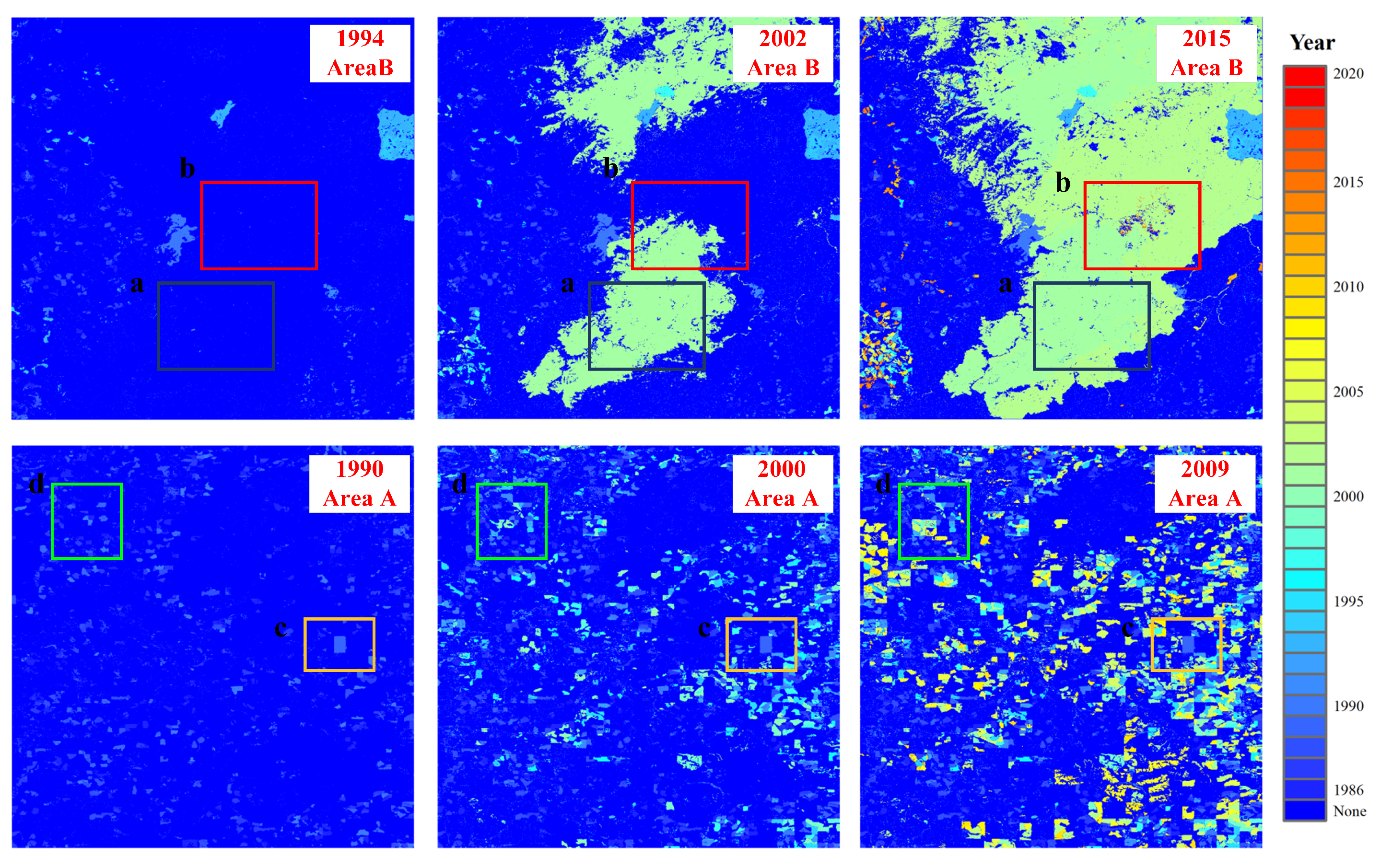
We mapped the disturbance point of areas A and B consecutively with the help of MT-CNN. To better illustrate the prediction accuracy of the proposed method. We created three accumulated forest disturbance maps for area A in the year 1994, 2002, and 2015, and for area B in the year 1990, 2000, and 2009 (as shown in Figure 8), respectively. For area A, we can see that fire disturbance (the Biscuit Complex wildfire (2002)) have occurred in the year 2002 for the black square window. It continuously expanded to larger areas, a specific disturbance region inside of red box have appeared in the year 2015 (the Buckskin wildfire (2015)). For area B, there are several deforestation events that happened inside of this area. At the beginning, a few number of disturbance pixels are identified in the year 1990. Then, a few disturbances are identified in 2000 with rectangular-like shapes, which mainly produced by timber harvest, as shown in the green and yellow box. In 2009, massive disturbances can be observed around the outskirts area of previous logging sites. These maps are consistent with the time of the disturbances observed by Google Earth. The mapping results indicate that the proposed MT-CNN is able to continuously detect the disturbance point regardless of the types.
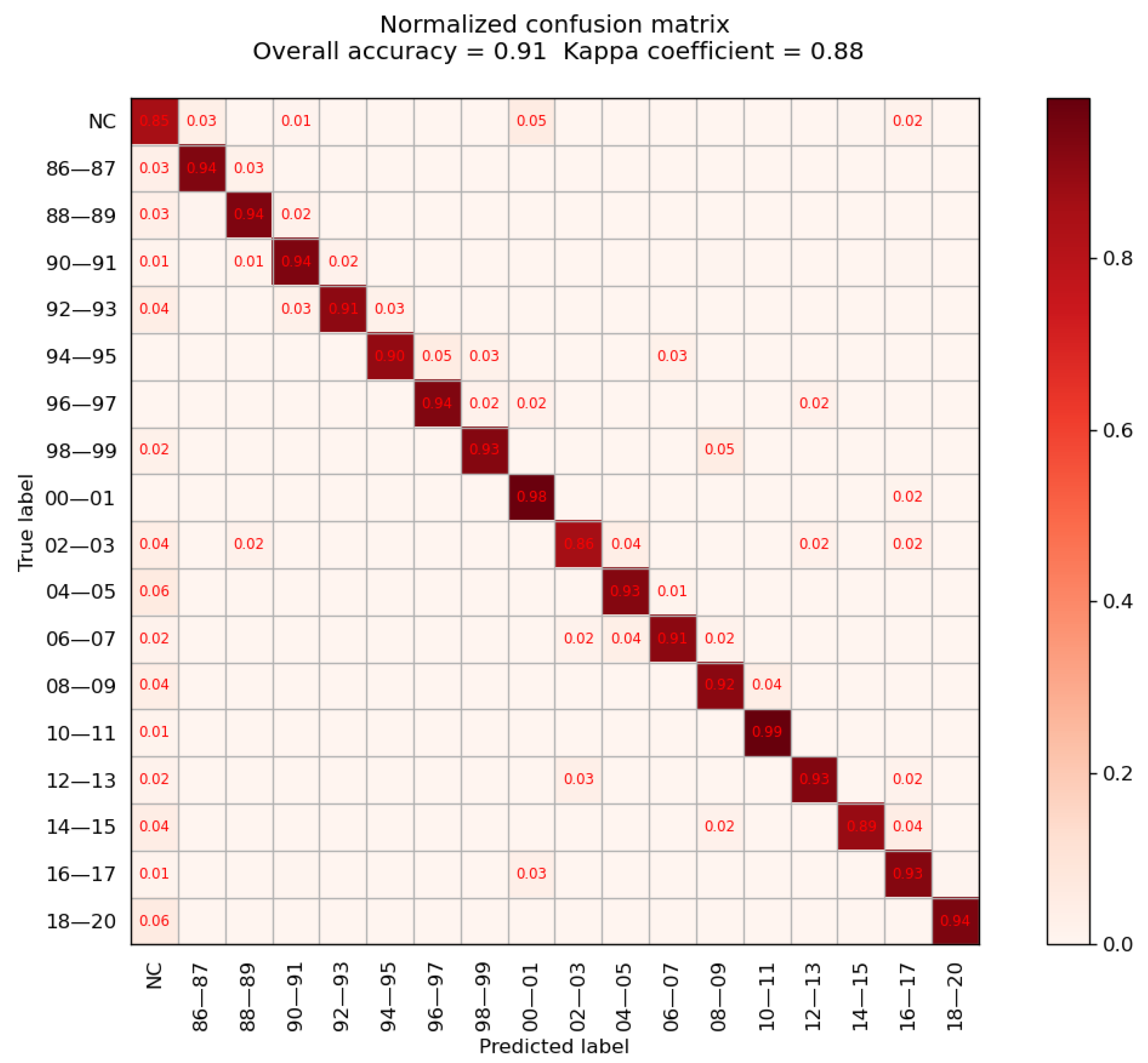
To quantitatively measure the accuracy of disturbance point detection, we compared the annotated label with the predicted output. For the annotated label, we extracted the staring magnitude as the standard disturbance point. Also, for the circumstance that disturbance happened more than once given a time-series signal, we only extracted the first disturbance point for comparison. The time span of our study area is more than 30 years; therefore, we re-grouped the detection results with 2-year bins for an easy plot. We used another annotated samples to test the accuracy of the proposed MT-CNN in disturbance point detection. Given the 2-year bin as a statistic unit, the confusion matrix in disturbance point detection is generated, as shown in Figure 9. The overall accuracy in terms of disturbance point detection reaches , and the kappa coefficient is 0.88. For the confusion matrix, the majority of detection accuracies are above . For instance, the disturbance point detection accuracy reaches around the year 2010–2011. Low-confident detection rates appeared at the beginning and end of time- series, where prior information is limited and coupled with significant noises. For the no-change (NC) class, the stable forests also demonstrated great variations in the time-series NBR index that inevitably lead to false predictions.
4.2.2. Disturbance Type Accuracy Analysis
Disturbance type identification is one of the most challenging tasks in time-series analysis. The proposed MT-CNN developed a multitemporal scheme to capture change patterns from various time-series fragments. To feed MT-CNN, the time-series fragments were extracted based on the disturbance point identified from the previous step. The accumulative disturbance maps on two areas (area A and area B in Figure 7) are demonstrated with two types of disturbance, that are, fire and harvest/deforestation, as shown in Figure 10. We visually inspected the disturbance type maps and found clear boundaries between stable forest and disturbances. For the left area B, the dominant disturbance type is fire and it is mainly covered by the mountain area, while with the right area A, the dominant disturbance type is deforestation caused by human intervention, as square-shaped logging sites can be clearly observed.
To quantitatively validate the disturbance type detection results, we used 5795 available test samples to calculate disturbance accuracy. For the classes of no change (stable forest), fire, and harvest/deforestation, the user accuracy is , , , and the producer accuracy is , , . The overall accuracy of disturbance type identification as high as , and the kappa coefficient is 0.85, as shown in Table 1. The results of disturbance type detection further proved the robustness of the MT-CNN regardless of the complex background.
4.2.3. Disturbance Frequency Accuracy Analysis
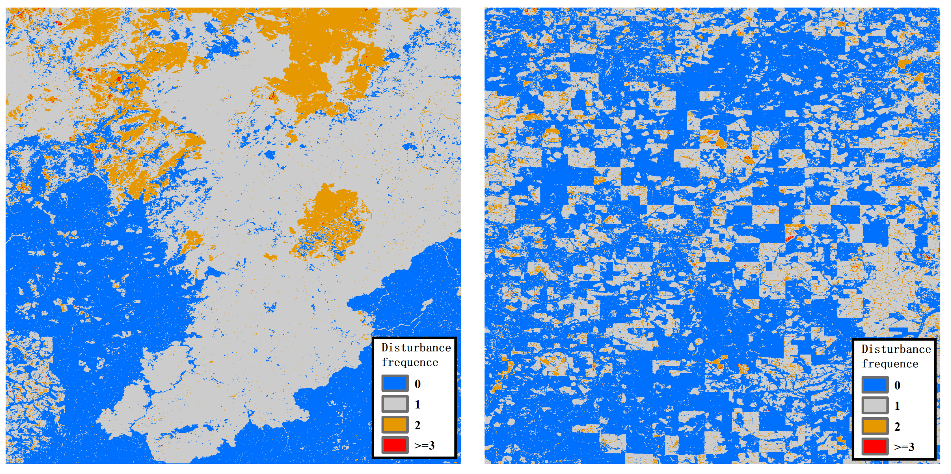
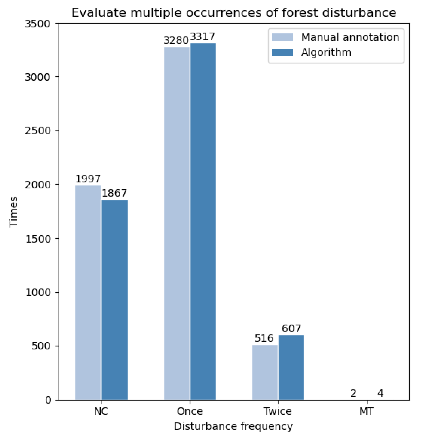
Compare to the disturbance point and type identification, the continuity of detection is another important indicator to evaluate the detection ability of the proposed method. To illustrate the continuity detection capability, we mapped the disturbance frequency for every single pixel on areas A and B, as shown in Figure 11. In this figure, we counted the disturbance times with one, two, and multiple (MT > 2) for each pixel, the statistical results are shown in the Figure 12. For the left area A, most disturbed areas have a one-time fire event, while inside the mountain area, 2-time disturbances also can be found. It indicates that this area suffers from continuous fire disturbances that significantly reduce the stability of the forest. Meanwhile, for the right area B, a large proportion of detected areas encountered more than 2-time disturbances. The reason for this phenomenon is probably the regular harvest of planted trees. From a quantitative point of view, we randomly selected 5795 test samples from areas A and B, and there were 3317 and 607 detected disturbances that occurred once or twice over the past 35 years. In general, the proposed method illustrated great robustness in multiple-disturbance detection.
5. Discussion
The proposed MT-CNN uses an integrated strategy to identify forest disturbances in terms of disturbance point, type, and frequency. Compared with the most existing forest disturbance detection strategies, the proposed method focuses on identifying the type of time-series fragments which include both decline and duration process. Since the disturbance point is determined, the time-series fragments with various lengths/scales can be fed into the MT-CNN for further type understanding. This multitemporal based forest disturbance detection strategy proved to be efficient at frequent, multiple-type disturbance identification. Still, the proposed method requires multitemporal inputs, which left an open question on temporal scale selection. In other words, how to choose the best temporal scale for disturbance type identification is remains unexploited. In addition, from the disturbance results of the USA west coast, we can observe the significant differences between the north and south region over the past 35 years in terms of forest disturbances. Also, the continuous fire disturbances happened inside of mountain areas, and the reason for this phenomenon is worth noticing. Therefore, in this section, we discussed two important factors that could impact the disturbance detection results.
5.1. Contribution of Multitemporal Scheme
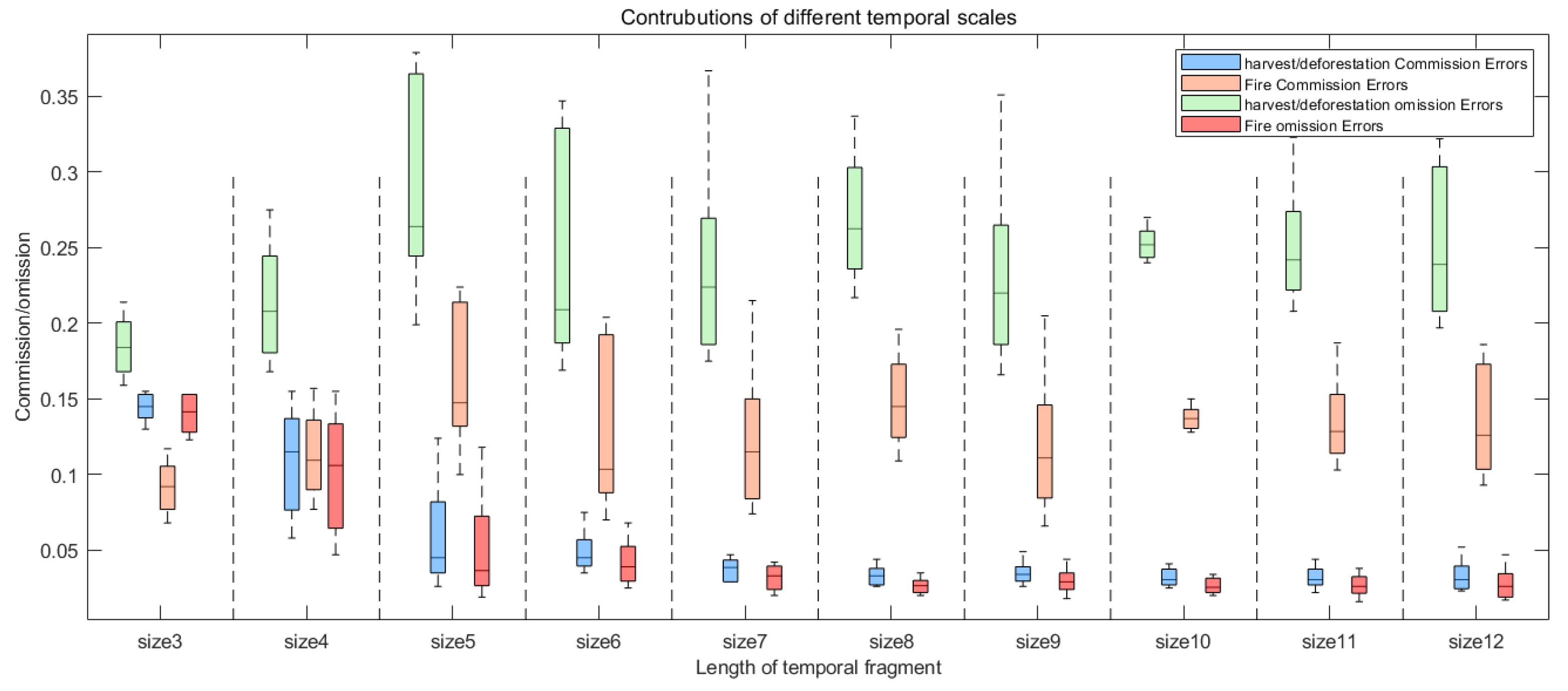
To quantify the impact factor of a multitemporal scheme for disturbance detection. We set up an ablation experiment with different lengths of time-series fragments as multitemporal inputs. For a specific length of the fragment, the MT-CNN is able to automatically adjusted to fit the dimension of input data. To train and test the accuracy of disturbance types, we split all available samples into and . To determine both the final estimate of the expected accuracy and the standard deviation, we ran this train-test process 10 times on every single temporal scale. The quantitative evaluation of prediction results is plotted in a boxplot as shown in Figure 13. In this figure, boxes show the median and interquartile range of commission and omission errors for fire or harvest/deforestation disturbance type given a specific temporal scale, and whiskers show full data range. In general, the commission error for harvest/deforestation is relatively lower than that of fire disturbances. For omission error, it shows the opposite trend. With the increasing size of the temporal fragment, the commission error of harvest/deforestation and the omission error of forest fire witnessed a slow decline trend, and the values stay around 0.1 without significant variations. However, for the commission error of the forest fire and the omission error of the harvest/deforestation, there are three distinct valleys on the temporal scale of 3–4, 6–7, and 9–10. Consequently, different scales temporal-series fragments have different abilities to distinguish different disturbances types.
Therefore, the multitemporal scheme is effective in terms of disturbance type identification. Specifically, for the fire disturbance, the predicted accuracies increase with the larger input temporal scale. Meanwhile, the decline disturbance is not sensitive to the temporal scale as it with smaller duration temporal window. The conclusion will further guide us to select proper temporal scales for various forest disturbances.
5.2. Influencing Factors of Forest Disturbance
The study area is located on the west coast of the USA, which is dominated by a Mediterranean climate. With the increasing crisis of global warming, this area is continuously impacted by heatwaves and wildfires. In the northern region of the study area, the low-altitude forests with intense human management are much more protected against wildfires, but regular tree harvesting is a major disturbance. The northwest region is the most stable region, and it greatly benefits from cooler temperatures and sufficient precipitation. By contrast, for the southern region, mountains with solid rocks and high-altitude drive plants tend to be extremely dry and flammable. From the previous disturbance maps, we can conclude that forests in the southern region continuously suffer from fire disturbances. The extremely large-scale wildfires broke out in the years 2002 and 2015. The frequency of fire disturbances in the southern mountain area is relatively high, especially for deep forest regions. Comparatively, for the northern region, most disturbances are forest decline caused by human activities. These harvest/deforestation regions are near to cities or towns, to where timber can be easily transported. However, the relationship between terrain features (such as DEM), weather indicators (precipitation and temperature), and disturbance frequency is needed to be deduced.
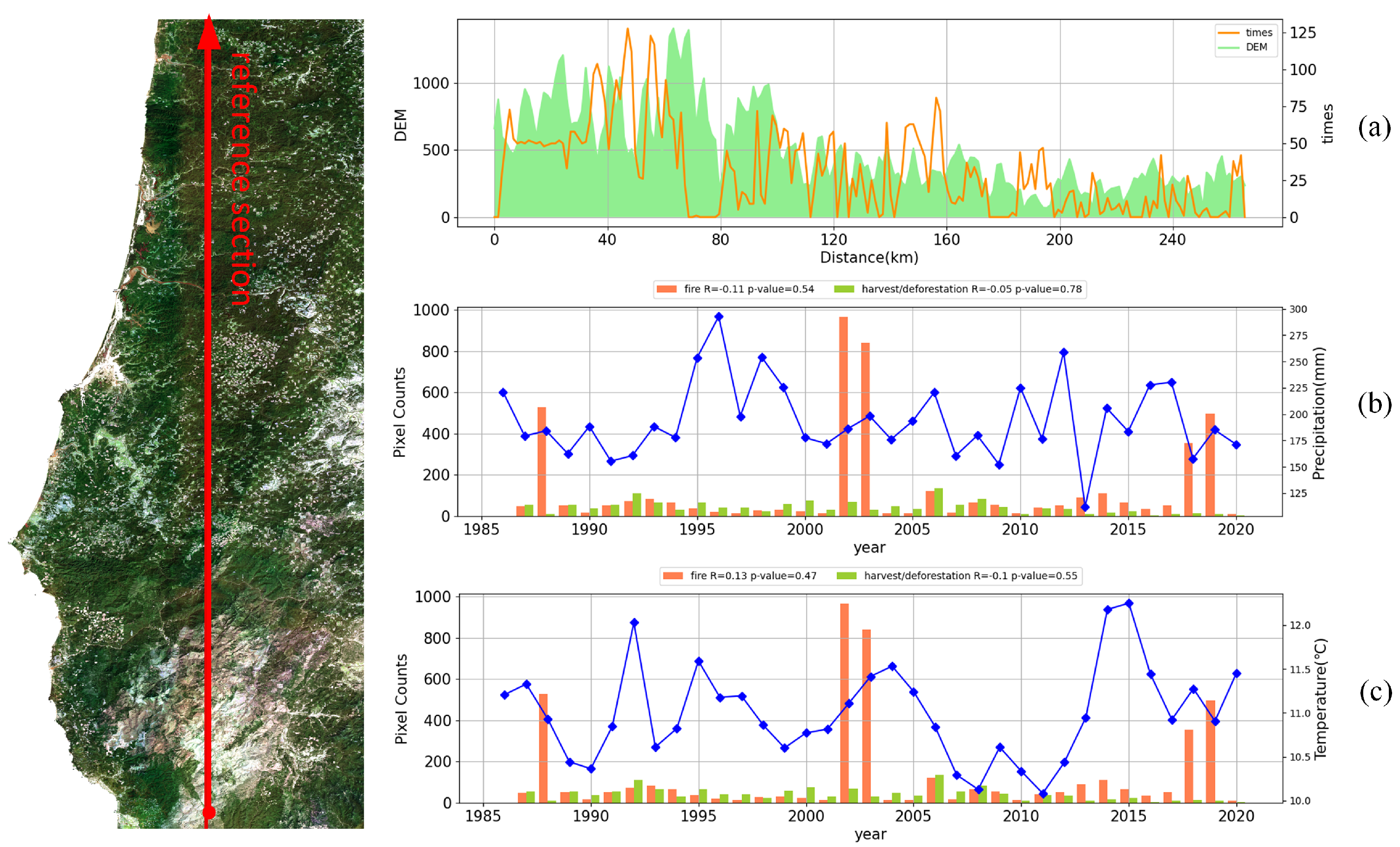
We obtained DEM, temperature and precipitation data on the GEE platform through two data sets named “PRISM Monthly Spatial Climate Dataset AN81m” and “NASADEM”.To determine the relationship between DEM and disturbance frequency, we have selected a representative “south-north” profile for quantitative analysis. To better represent the statistical results, we set the statistical bin to 50 pixels. That is, the DEM is the average value of all the 50 pixels. And, the number of disturbances was summarized from 50 pixels for better understanding. Began with the south region, we can see that a sharp increase in DEM as it is the mountain region. In the meantime, a sharp increase also can be observed in the number of disturbances inside of this region. The highest disturbance number reaches 125 times for a statistical unit over the past 35 years. Then, the number of disturbances almost reaches 0 as DEM drops to 0. It means that the valley area with sufficient water and cooler temperature will prevent wildfire expansion. For DEM in the range of 0–500 m, the disturbances occurred without significant patterns. Statistical units that far than 160 km demonstrate a much more stable curve than the southern regions. While the disturbance type of this region is mainly harvest/deforestation with human intervention. In general, we can conclude that the number of disturbances roughly coincided with the distribution of DEM. That is, the higher DEM may suffer frequent disturbances than the plain area.
As the study area is mainly with the Mediterranean climate, scarce rains in hot summer usually coexistence with severe fire disturbances. We collected the annual precipitation rates over the last 35 years, and plotted it with the occurrence of observed disturbances, as shown in Figure 14. The highest precipitation rate reaches almost 300 mm in 1996 that coupled with the lowest frequency of fire disturbance. On the contrary, the minimum annual precipitation is about 50 mm which appeared in 2014 within this study area. The medium precipitation is around 175 mm per year, and five large-scale fire disturbances appeared in the year of 1988, 2002, 2003, 2018, and 2019, respectively. Comparatively, the harvest/deforestation is relatively stable that varies from the range of 0–100 cases that happened in the 300 km profile over the last 35 years. After 2015, the deforestation caused by human activities has significantly dropped, while fire disturbance continuously increases. From the perspective of temperature variation, we also plotted the mean annual temperature over the selected profile. The overall trend of the plotted curve demonstrates small variations between 10 to 12 . And 2015, 2014, and 1992 are the top three hottest years, while 2011, 2008, and 1990 are the top three coolest years. The highest temperature almost reaches 12.5 in 2015 and the coolest temperature near to 10 in 2011. Coupled with the precipitation information, the frequency of fire disturbance significantly increases when little rain with high temperature both appeared within a year. Although the scorching heat did not immediately cause heat fire in 2015, the dryer soil and dead trees become one of the most important factors for wildfire outbroke in 2018 and 2019. Therefore, both DEM, precipitation, and temperature potentially impact the frequency of forest disturbance in the west coast region of the USA. The reason behind this phenomenon is worth being quantitatively evaluated in future studies.
6. Conclusions
Forest is one of the fundamental elements for human survival on Earth. With ever-increasing global warming and land detrition, timely and accurate identification of forest disturbances in terms of their location, type, and frequency are urgently needed. Aiming to detect forest disturbances from long time-series satellite data, we developed a multitemporal convolutional neural network (MT-CNN) to automatically identify forest disturbances with the feature of the beginning point, type, and frequency. The main contribution of this method is threshold-free multiscale identification of forest disturbances, regardless of duration periods variations of different events. To validate the performance of the proposed method, we selected a large-scale study area of the west coast area of the USA. For the 35-year time-series data, we identified forest disturbances with respect to their occurrence time, type, and frequency for each pixel. The overall accuracy reaches compared to the manually labeled data. From the forest disturbance map, we also concluded that forest disturbances coupled with several indicators including DEM, precipitation, and temperature.
Author Contributions
Conceptualization, X.C. (Xi Chen) and W.Z.; methodology, X.C. (Xi Chen) and W.Z.; data analyses, J.C., Y.Q. and D.W.; writing—original draft preparation, X.C. (Xi Chen) and W.Z.; writing—review and editing, X.C. (Xi Chen), W.Z. and J.C.; visualization, X.C. (Xi Chen), W.Z., Y.Q., D.W. and J.C.; supervision, X.C. (Xuehong Chen), W.Z. and J.C.; project administration, X.C. (Xuehong Chen), W.Z. and J.C. All authors have read and agreed to the published version of the manuscript.
Funding
This research project was funded by National Natural Science Foundation of China (No. 41871224), National Key Program of China (2018YFC1508903), and Beijing Municipal Natural Science Foundation (No. 4214065).
Conflicts of Interest
The authors declare no conflict of interest.
References
- Kurz, W.; Dymond, C.; White, T.; Stinson, G.; Shaw, C.; Rampley, G.; Smyth, C.; Simpson, B.; Neilson, E.; Trofymow, J. CBM-CFS3: A model of carbon-dynamics in forestry and land-use change implementing IPCC standards. Ecol. Model. 2009, 220, 480–504. [Google Scholar] [CrossRef]
- Li, R.; Buongiorno, J.; Turner, J.A.; Zhu, S.; Prestemon, J. Long-term effects of eliminating illegal logging on the world forest industries, trade, and inventory. For. Policy Econ. 2008, 10, 480–490. [Google Scholar] [CrossRef]
- Cohen, W.B.; Healey, S.P.; Yang, Z.; Zhu, Z.; Gorelick, N. Diversity of algorithm and spectral band inputs improves Landsat monitoring of forest disturbance. Remote Sens. 2020, 12, 1673. [Google Scholar] [CrossRef]
- Mirabel, A.; Hérault, B.; Marcon, E. Diverging taxonomic and functional trajectories following disturbance in a Neotropical forest. Sci. Total Environ. 2020, 720, 137397. [Google Scholar] [CrossRef] [PubMed]
- Zhu, F.; Wang, H.; Li, M.; Diao, J.; Shen, W.; Zhang, Y.; Wu, H. Characterizing the effects of climate change on short-term post-disturbance forest recovery in southern China from Landsat time-series observations (1988–2016). Front. Earth Sci. 2020, 14, 816–827. [Google Scholar] [CrossRef]
- Senf, C.; Pflugmacher, D.; Hostert, P.; Seidl, R. Using Landsat time series for characterizing forest disturbance dynamics in the coupled human and natural systems of Central Europe. ISPRS J. Photogramm. Remote Sens. 2017, 130, 453–463. [Google Scholar] [CrossRef] [PubMed]
- Cohen, W.B.; Goward, S.N. Landsat’s role in ecological applications of remote sensing. Bioscience 2004, 54, 535–545. [Google Scholar] [CrossRef]
- Hansen, M.C.; Potapov, P.V.; Moore, R.; Hancher, M.; Turubanova, S.A.; Tyukavina, A.; Thau, D.; Stehman, S.; Goetz, S.J.; Loveland, T.R. High-resolution global maps of 21st-century forest cover change. Science 2013, 342, 850–853. [Google Scholar] [CrossRef] [Green Version]
- Wulder, M.A.; White, J.C.; Goward, S.N.; Masek, J.G.; Irons, J.R.; Herold, M.; Cohen, W.B.; Loveland, T.R.; Woodcock, C.E. Landsat continuity: Issues and opportunities for land cover monitoring. Remote Sens. Environ. 2008, 112, 955–969. [Google Scholar] [CrossRef]
- Kennedy, R.E.; Andréfouët, S.; Cohen, W.B.; Gómez, C.; Griffiths, P.; Hais, M.; Healey, S.P.; Helmer, E.H.; Hostert, P.; Lyons, M.B. Bringing an ecological view of change to Landsat-based remote sensing. Front. Ecol. Environ. 2014, 12, 339–346. [Google Scholar] [CrossRef]
- Cohen, W.B.; Yang, Z.; Healey, S.P.; Kennedy, R.E.; Gorelick, N. A LandTrendr multispectral ensemble for forest disturbance detection. Remote Sens. Environ. 2018, 205, 131–140. [Google Scholar] [CrossRef]
- Meng, Y.; Liu, X.; Ding, C.; Xu, B.; Zhou, G.; Zhu, L. Analysis of ecological resilience to evaluate the inherent maintenance capacity of a forest ecosystem using a dense Landsat time series. Ecol. Inform. 2020, 57, 101064. [Google Scholar] [CrossRef]
- Huang, C.; Goward, S.N.; Schleeweis, K.; Thomas, N.; Masek, J.G.; Zhu, Z. Dynamics of national forests assessed using the Landsat record: Case studies in eastern United States. Remote Sens. Environ. 2009, 113, 1430–1442. [Google Scholar] [CrossRef]
- Myroniuk, V.; Bilous, A.; Khan, Y.; Terentiev, A.; Kravets, P.; Kovalevskyi, S.; See, L. Tracking Rates of Forest Disturbance and Associated Carbon Loss in Areas of Illegal Amber Mining in Ukraine Using Landsat Time Series. Remote Sens. 2020, 12, 2235. [Google Scholar] [CrossRef]
- Kennedy, R.E.; Cohen, W.B.; Schroeder, T.A. Trajectory-based change detection for automated characterization of forest disturbance dynamics. Remote Sens. Environ. 2007, 110, 370–386. [Google Scholar] [CrossRef]
- Kennedy, R.E.; Yang, Z.; Cohen, W.B. Detecting trends in forest disturbance and recovery using yearly Landsat time series: 1. LandTrendr—Temporal segmentation algorithms. Remote Sens. Environ. 2010, 114, 2897–2910. [Google Scholar] [CrossRef]
- Maus, V.; Câmara, G.; Cartaxo, R.; Sanchez, A.; Ramos, F.M.; De Queiroz, G.R. A time-weighted dynamic time warping method for land-use and land-cover mapping. IEEE J. Sel. Top. Appl. Earth Obs. Remote Sens. 2016, 9, 3729–3739. [Google Scholar] [CrossRef]
- Yan, J.; Wang, L.; Song, W.; Chen, Y.; Chen, X.; Deng, Z. A time-series classification approach based on change detection for rapid land cover mapping. ISPRS J. Photogramm. Remote Sens. 2019, 158, 249–262. [Google Scholar] [CrossRef]
- Verbesselt, J.; Hyndman, R.; Zeileis, A.; Culvenor, D. Phenological change detection while accounting for abrupt and gradual trends in satellite image time series. Remote Sens. Environ. 2010, 114, 2970–2980. [Google Scholar] [CrossRef] [Green Version]
- Verbesselt, J.; Zeileis, A.; Herold, M. Near real-time disturbance detection using satellite image time series. Remote Sens. Environ. 2012, 123, 98–108. [Google Scholar] [CrossRef]
- Zhu, Z.; Woodcock, C.E. Continuous change detection and classification of land cover using all available Landsat data. Remote Sens. Environ. 2014, 144, 152–171. [Google Scholar] [CrossRef] [Green Version]
- Zhu, Z.; Woodcock, C.E.; Holden, C.; Yang, Z. Generating synthetic Landsat images based on all available Landsat data: Predicting Landsat surface reflectance at any given time. Remote Sens. Environ. 2015, 162, 67–83. [Google Scholar] [CrossRef]
- Ye, S.; Rogan, J.; Zhu, Z.; Eastman, J.R. A near-real-time approach for monitoring forest disturbance using Landsat time series: Stochastic continuous change detection. Remote Sens. Environ. 2021, 252, 112167. [Google Scholar] [CrossRef]
- Zhu, Z.; Fu, Y.; Woodcock, C.E.; Olofsson, P.; Vogelmann, J.E.; Holden, C.; Wang, M.; Dai, S.; Yu, Y. Including land cover change in analysis of greenness trends using all available Landsat 5, 7, and 8 images: A case study from Guangzhou, China (2000–2014). Remote Sens. Environ. 2016, 185, 243–257. [Google Scholar] [CrossRef] [Green Version]
- Zhu, Z.; Zhang, J.; Yang, Z.; Aljaddani, A.H.; Cohen, W.B.; Qiu, S.; Zhou, C. Continuous monitoring of land disturbance based on Landsat time series. Remote Sens. Environ. 2020, 238, 111116. [Google Scholar] [CrossRef]
- Shimizu, K.; Ota, T.; Mizoue, N.; Yoshida, S. A comprehensive evaluation of disturbance agent classification approaches: Strengths of ensemble classification, multiple indices, spatio-temporal variables, and direct prediction. ISPRS J. Photogramm. Remote Sens. 2019, 158, 99–112. [Google Scholar] [CrossRef]
- Zhan, Y.; Fu, K.; Yan, M.; Sun, X.; Wang, H.; Qiu, X. Change detection based on deep siamese convolutional network for optical aerial images. IEEE Geosci. Remote Sens. Lett. 2017, 14, 1845–1849. [Google Scholar] [CrossRef]
- Kislov, D.E.; Korznikov, K.A.; Altman, J.; Vozmishcheva, A.S.; Krestov, P.V. Extending deep learning approaches for forest disturbance segmentation on very high-resolution satellite images. Remote Sens. Ecol. Conserv. 2021, 7, 355–368. [Google Scholar] [CrossRef]
- Yang, Q.; Shi, L.; Han, J.; Yu, J.; Huang, K. A near real-time deep learning approach for detecting rice phenology based on UAV images. Agric. For. Meteorol. 2020, 287, 107938. [Google Scholar] [CrossRef]
- Ye, L.; Gao, L.; Marcos-Martinez, R.; Mallants, D.; Bryan, B.A. Projecting Australia’s forest cover dynamics and exploring influential factors using deep learning. Environ. Model. Softw. 2019, 119, 407–417. [Google Scholar] [CrossRef]
- Kong, Y.-L.; Huang, Q.; Wang, C.; Chen, J.; Chen, J.; He, D. Long short-term memory neural networks for online disturbance detection in satellite image time series. Remote Sens. 2018, 10, 452. [Google Scholar] [CrossRef] [Green Version]
- Ban, Y.; Zhang, P.; Nascetti, A.; Bevington, A.R.; Wulder, M.A. Near real-time wildfire progression monitoring with Sentinel-1 SAR time series and deep learning. Sci. Rep. 2020, 10, 1322. [Google Scholar] [CrossRef] [PubMed] [Green Version]
- Kennedy, R.E.; Yang, Z.; Cohen, W.B.; Pfaff, E.; Braaten, J.; Nelson, P. Spatial and temporal patterns of forest disturbance and regrowth within the area of the Northwest Forest Plan. Remote Sens. Environ. 2012, 122, 117–133. [Google Scholar] [CrossRef]
- Bright, B.C.; Hudak, A.T.; Kennedy, R.E.; Braaten, J.D.; Khalyani, A.H. Examining post-fire vegetation recovery with Landsat time series analysis in three western North American forest types. Fire Ecol. 2019, 15, 8. [Google Scholar] [CrossRef] [Green Version]
- Turner, M.G. Disturbance and landscape dynamics in a changing world. Ecology 2010, 91, 2833–2849. [Google Scholar] [CrossRef] [PubMed] [Green Version]
- Rodman, K.C.; Andrus, R.A.; Veblen, T.T.; Hart, S. Disturbance detection in landsat time series is influenced by tree mortality agent and severity, not by prior disturbance. Remote Sens. Environ. 2021, 254, 112244. [Google Scholar] [CrossRef]
- Chen, D.; Fu, C.; Hall, J.V.; Hoy, E.E.; Loboda, T.V. Spatio-temporal patterns of optimal Landsat data for burn severity index calculations: Implications for high northern latitudes wildfire research. Remote Sens. Environ. 2021, 258, 112393. [Google Scholar] [CrossRef]
- Gao, Y.; Solórzano, J.V.; Quevedo, A.; Loya-Carrillo, J.O. How BFAST Trend and Seasonal Model Components Affect Disturbance Detection in Tropical Dry Forest and Temperate Forest. Remote Sens. 2021, 13, 2033. [Google Scholar] [CrossRef]
- Roy, D.P.; Kovalskyy, V.; Zhang, H.; Vermote, E.F.; Yan, L.; Kumar, S.; Egorov, A. Characterization of Landsat-7 to Landsat-8 reflective wavelength and normalized difference vegetation index continuity. Remote Sens. Environ. 2016, 185, 57–70. [Google Scholar] [CrossRef] [Green Version]
- DeVries, B.; Decuyper, M.; Verbesselt, J.; Zeileis, A.; Herold, M.; Joseph, S. Tracking disturbance-regrowth dynamics in tropical forests using structural change detection and Landsat time series. Remote Sens. Environ. 2015, 169, 320–334. [Google Scholar] [CrossRef]
- Cohen, W.B.; Yang, Z.; Kennedy, R. Detecting trends in forest disturbance and recovery using yearly Landsat time series: 2. TimeSync—Tools for calibration and validation. Remote Sens. Environ. 2010, 114, 2911–2924. [Google Scholar] [CrossRef]
Figure 1.
Study on west coast area of USA. Area A is dominated by forest decline, while Area B is dominated by wildfires.
Figure 1.
Study on west coast area of USA. Area A is dominated by forest decline, while Area B is dominated by wildfires.

Figure 2.
The typical time-series curves for different types of forest disturbances. (a) represents fire disturbance while (b) represents harvest/deforestation.
Figure 2.
The typical time-series curves for different types of forest disturbances. (a) represents fire disturbance while (b) represents harvest/deforestation.

Figure 3.
Two annotated areas with different types of forest disturbances. Harvest/deforestation disturbance samples are shown in left, while fire disturbance samples are shown in right.
Figure 3.
Two annotated areas with different types of forest disturbances. Harvest/deforestation disturbance samples are shown in left, while fire disturbance samples are shown in right.

Figure 4.
Flowchart of proposed integrated MT-CNN. (1) yearly composite data are prepared for analysis; (2) disturbance point is detected with sliding window technique; (3) disturbance type recognition with multitemporal time-series fragments.
Figure 4.
Flowchart of proposed integrated MT-CNN. (1) yearly composite data are prepared for analysis; (2) disturbance point is detected with sliding window technique; (3) disturbance type recognition with multitemporal time-series fragments.

Figure 5.
Flowchart of the multitemporal CNN framework.

Figure 6.
(a–c) Disturbance mapping results on disturbance point, type, and frequency.

Figure 7.
Finer-scale illustration of forest disturbance events with specific year.

Figure 8.
Disturbance point detection results on area A and B. For area A, maps with forest fire in years of 1994–2002–2015 are illustrated. For area B, maps with harvest/deforestation in years of 1990–2000–2009 are illustrated.
Figure 8.
Disturbance point detection results on area A and B. For area A, maps with forest fire in years of 1994–2002–2015 are illustrated. For area B, maps with harvest/deforestation in years of 1990–2000–2009 are illustrated.

Figure 9.
Confusion matrix of disturbance point detection from 1986 to 2020.

Figure 10.
Disturbance type identification on area A and area B. Left area B is dominated by forest fire, while right area A is dominated by harvest/deforestation.
Figure 10.
Disturbance type identification on area A and area B. Left area B is dominated by forest fire, while right area A is dominated by harvest/deforestation.

Figure 11.
Mapping results of forest disturbance frequencies. Left area B is dominated by 1 or 2 times disturbances while right area A dominated with more than 3 times number of forest disturbances within 35 years.
Figure 11.
Mapping results of forest disturbance frequencies. Left area B is dominated by 1 or 2 times disturbances while right area A dominated with more than 3 times number of forest disturbances within 35 years.

Figure 12.
Statistical results on multiple disturbance with 5795 selected test samples.

Figure 13.
Overall accuracy regarding disturbance types with different lengths of temporal fragment.
Figure 13.
Overall accuracy regarding disturbance types with different lengths of temporal fragment.

Figure 14.
(a–c) Influences of terrain and weather factors on different types of forest disturbances.
Figure 14.
(a–c) Influences of terrain and weather factors on different types of forest disturbances.


Table 1.
Accuracies of disturbance type identification.
| Manual Annotation | Users Accuracy | |||
|---|---|---|---|---|
| No Change | Fire | Harvest/Deforestation | ||
| Algorithm | ||||
| No change | 1749 | 4 | 114 | |
| Fire | 177 | 1952 | 177 | |
| harvest/deforestation | 71 | 44 | 1507 | |
| Producers accuracy | ||||
| Overall users accuracy | Overall accuracy | |||
| Overall producers accuracy | Kappa coefficient | |||
Publisher’s Note: MDPI stays neutral with regard to jurisdictional claims in published maps and institutional affiliations. |
© 2021 by the authors. Licensee MDPI, Basel, Switzerland. This article is an open access article distributed under the terms and conditions of the Creative Commons Attribution (CC BY) license (https://creativecommons.org/licenses/by/4.0/).
Share and Cite
MDPI and ACS Style
Chen, X.; Zhao, W.; Chen, J.; Qu, Y.; Wu, D.; Chen, X. Mapping Large-Scale Forest Disturbance Types with Multi-Temporal CNN Framework. Remote Sens. 2021, 13, 5177. https://0-doi-org.brum.beds.ac.uk/10.3390/rs13245177
AMA Style
Chen X, Zhao W, Chen J, Qu Y, Wu D, Chen X. Mapping Large-Scale Forest Disturbance Types with Multi-Temporal CNN Framework. Remote Sensing. 2021; 13(24):5177. https://0-doi-org.brum.beds.ac.uk/10.3390/rs13245177
Chicago/Turabian StyleChen, Xi, Wenzhi Zhao, Jiage Chen, Yang Qu, Dinghui Wu, and Xuehong Chen. 2021. "Mapping Large-Scale Forest Disturbance Types with Multi-Temporal CNN Framework" Remote Sensing 13, no. 24: 5177. https://0-doi-org.brum.beds.ac.uk/10.3390/rs13245177
Note that from the first issue of 2016, this journal uses article numbers instead of page numbers. See further details here.