1. Introduction
Hygroscopic aerosol particles serve as the cloud condensation nuclei (CCN) for cloud drop formation. The first aerosol indirect effect (Twomey effect) describes the decrease of droplet size with increasing CCN number given the same liquid water content, leading to higher cloud albedo [
1]. The second indirect effect (Albrecht effect) further concerns the delay of drizzle formation, owing to the less efficient collision coalescence processes by smaller droplets, leading to enhanced cloud water path and longer cloud lifetime [
2]. On top of these effects, the overall responses of cloud to aerosols are modulated by the interplay among cloud dynamics, macrophysical and microphysical processes, and the influence of the ambient environment on cloud structure. Therefore, they are highly variable for different cloud regimes [
3,
4,
5].
For shallow clouds, previous studies identified the importance of evaporation-entrainment feedback to aerosol–cloud interactions. As droplet evaporation is enhanced for smaller cloud droplets, the stronger evaporative cooling promotes the entrainment of the unsaturated ambient air, leading to a further decrease in cloud water content and cloud albedo [
3,
6,
7,
8]. Such positive feedback can partially compensate for the increase in cloud albedo by the Twomey effect [
9,
10] and is, therefore, a critical process for determining the response of non-precipitating shallow clouds to increasing CCN [
11]. For precipitating shallow cumulus, however, the inhibition of drizzle formation can effectively accumulate more cloud water content through the cloud lifetime effect [
3], leading to an overall positive change in liquid water amount. The cloud optical depth and reflectivity of precipitating cloud are, therefore, more sensitive to aerosol changes [
12].
Chen et al. [
12] identified how ambient environment conditions modulate the susceptibility of cloud micro- and macro-physical properties to aerosol amounts for global marine warm clouds by collocating observations from several NASA A-Train satellites. They found that the free tropospheric humidity (RH
ft) and lower troposphere stability (LTS) play a key role in the sensitivity of cloud properties to increasing aerosols. In an unstable (i.e., lower LTS) environment, the inversion at the boundary layer top is weaker and, thus, more favorable for cloud-top entrainment; as a result, the marine warm clouds in the unstable condition reveal lower sensitivities to increased aerosols. For higher free-troposphere humidity, the cloud water path of precipitating warm clouds increases with increasing aerosol and is more sensitive compared to the drier environment, while the non-precipitating clouds exhibit decreasing cloud water amount with increasing aerosols but are less sensitive compared to a drier condition.
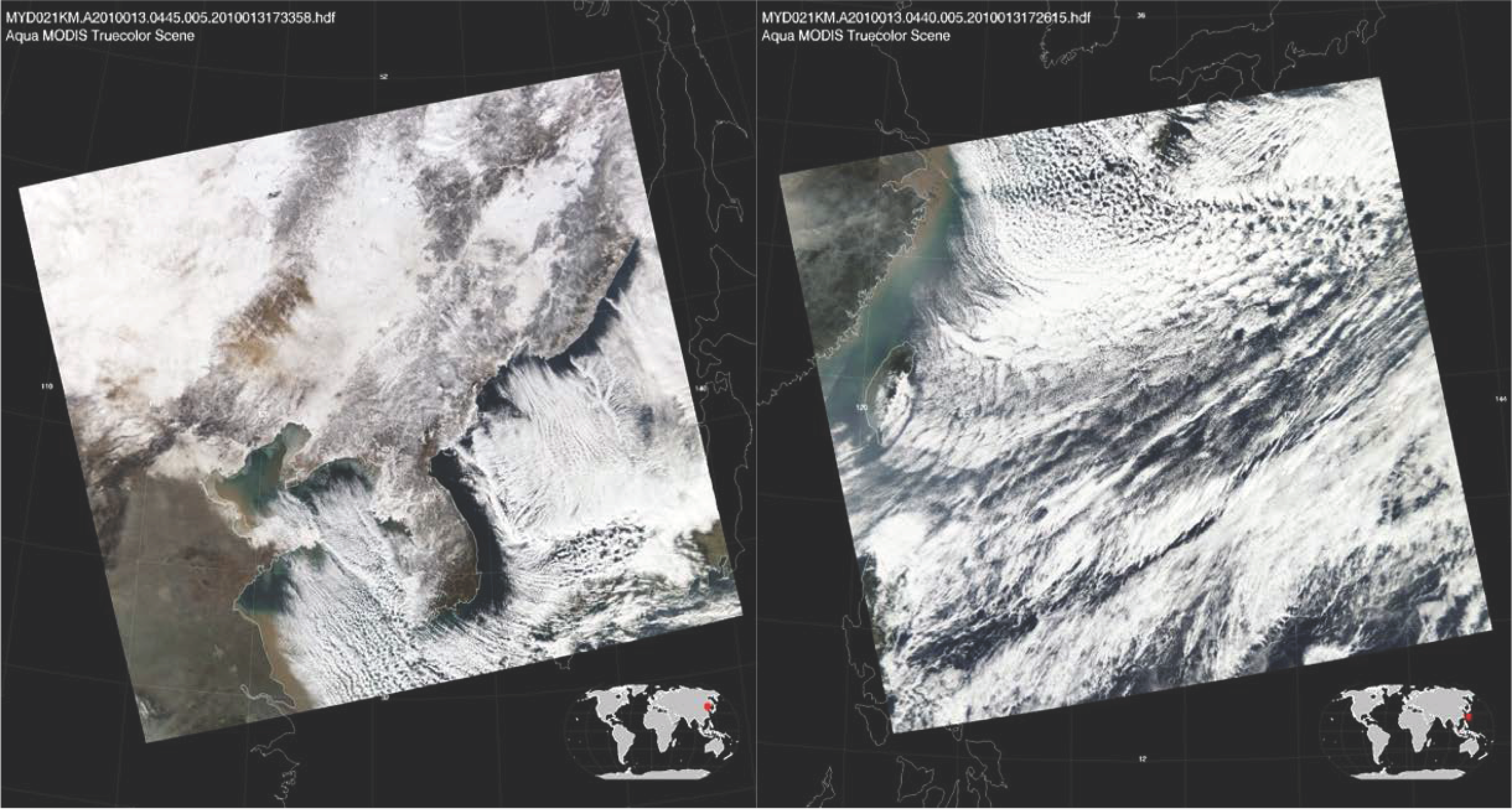
Over the East Asian monsoon region, marine warm clouds frequently occur in wintertime and springtime, but their appearance is more transient and closely tied to the variation of synoptic weather [
13,
14]. Especially during the cold-surge outbreak events, marine warm clouds can be clearly identified in satellite images, as shown in the example in
Figure 1. The critical environmental parameter for the formation of the marine warm clouds in this region is, therefore, different from the more persistent stratocumulus deck in the eastern Pacific and southeastern Atlantic. The SST over the Western Pacific is generally higher due to the Kuroshio current.
During the winter monsoon season, the large-scale subsidence leads to the capping inversion over the marine boundary layer, which favors the formation of the stratocumulus clouds. When the continental high-pressure systems propagate southeastward from the Asian Continent into the Yellow Sea and the East China Sea, the low-level cold air is quickly advected over the warm ocean surface. The air–sea temperature difference can be over 10 degrees over the areas of the Kuroshio warm current. The low clouds are formed in this marine boundary layer that is unstable in the near-surface and topped by the inversion due to strong subsidence of the continental high pressure. Koike et al. [
15,
16] used the near-surface stability (NSS) to quantify the warm sea surface destabilization effect, while Wood and Bretherton [
17] pointed out that the intensity of the capping inversion over the moist environment can be more relevantly represented by the estimated inversion strength (EIS).
As the near-surface stability and subsidence change along the path of the cold air advection during the cold air outbreak in East Asia, the cloud structure also varies from the cloud streets in the near-coastal ocean to the more cumuli form or open cell structure in the downstream ocean (
Figure 1). Liu et al. [
13] identified how the cloud top height and hydrometeor type transition along with the SST conditions over this region using the retrieval products from the CloudSat and Cloud-Aerosol Lidar and Infrared Pathfinder Satellite (CALIPSO). From cold to warm SST, the cloud top height increases, the cloud structure transitions from more stratiform to more convective, the hydrometeor composition changes from ice-phase dominant to mixtures of liquid cloud and raindrops, and the probability of precipitation also increases.
In the East Asian monsoon region, winter and spring are also the seasons of active aerosol pollution. Koike et al. [
15,
16] reported that the low-level winds during the cold air outbreak can quickly transport the aerosols from major anthropogenic emission source areas in northern China to the western Pacific, while the cold advection also destabilizes the marine boundary layer. They found that the near-surface instability and the increasing aerosols together can lead to a significant increase in cloud drop number, as well as higher cloud optical depth and reflectivity. Therefore, it is worthy to further delineate the effects of near-surface stability, inversion strength, and aerosols to cloud physical properties.
The present study investigated the response of marine warm clouds to aerosols over the East Asian Monsoon region during winter and spring using satellite products in the A-Train constellation and the reanalysis data. The data from CloudSat, MODIS, and CALIPSO (Cloud-Aerosol Lidar and Infrared Pathfinder Satellite) during the years 2006 to 2010 were collocated to identify the target single-layer marine warm cloud over the Northwestern Pacific, in order to analyze how clouds vary with environmental conditions, as well as how aerosol–cloud interactions may change with different precipitation statuses and environmental regimes. The data sets and data-processing procedures are introduced in
Section 2. The observed seasonal mean spatial distribution of marine warm clouds, ambient environment, and aerosol optical depths, as well as the susceptibility of cloud properties to aerosols, are described in
Section 3.
Section 4 and
Section 5 are discussions and the concluding remarks, respectively.
2. Data and Methods
The co-located satellite datasets from multiple data products used in this study were provided by Chen et al. [
12], and the major analysis was focusing on the winter (DJF) and spring (MAM) from 2006 to 2010 in the domain: 0–50
N, 100–140
E. All the data products used in this study are listed in
Table 1.
2.1. Aerosol and Cloud Data
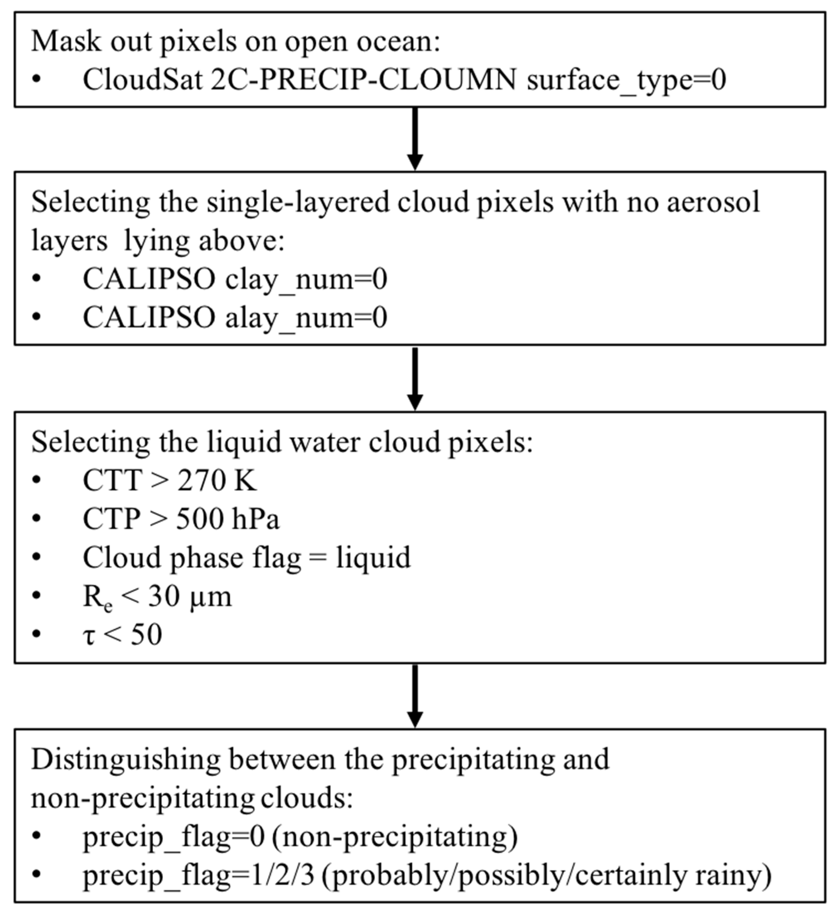
The cloud layer and aerosol layer flags obtained from CALIPSO Lidar Level 2 5-km Cloud and Aerosol Layer product version 3.01 [
18] were used to select the single-layered marine warm cloud pixels with no aerosol layers lying above.
The surface_type flag obtained from CloudSat 2C-PRECIP-COLUMN was used to select the pixels in the open ocean with no sea ice (surface_type = 0). The precip_flag was also applied to distinguish between the precipitating and non-precipitating cloud pixels: precip_flag = 0 indicates that no precipitation was detected, and precip_flag = 1, 2, and 3 suggest that it is possibly, probably, and certainly rainy, respectively.
The cloud optical properties were obtained from the Level 2 MODIS cloud products on the Aqua satellite (MYD06), including a 3.7-μm cloud droplet effective radius (Re), cloud optical depth (τ), cloud fraction (CF), cloud-top pressure (CTP), and cloud-top temperature. The derived liquid water path (LWP) = (2/3)Reρ
lτ, where ρ
l is liquid water density [
12].
To remove the ice and the mixed-phase clouds’ pixels, we used the cloud top pressure and temperature from the MYD06 product to identify warm liquid clouds with cloud top pressures greater than 500 hPa and cloud top temperatures exceeding 270 K [
12]. The Cloud albedo was derived based on CERES top of atmosphere short-wave radiative flux acquired from the CALIPSO-CloudSat-CERES-MODIS (CCCM) product [
12].
The 0.55-μm aerosol optical depth (AOD) was obtained from the Level 3 MODIS (MYD08) data product. In this study, we also used the Aerosol index (AI) [
12] as the proxy of the number of cloud condensation nuclei (CCN), which were defined as:
AI = AOD × Ångström exponent
Since AOD varies with the wavelength of the incident light, the relationship between the aerosol optical depth and the wavelength of light is described by the following equation:
, where
τλ and
τλ0 are the aerosol optical depth at the wavelength
λ and
λ0, respectively. The
α is the Ångström exponent. In this study, the Ångström exponent was calculated based on 0.55 μm and 0.867 μm AOD [
12]. The Ångström exponent offers the information of the particles’ size: the larger the exponent, the smaller the particles.
2.2. Environmental Parameters
The atmospheric environmental parameters such as temperature, pressure, and specific humidity were acquired from ECMWF-AUX. In an attempt to investigate the effect of the atmospheric environmental condition on aerosol–cloud interactions, the dataset was divided into different environmental regimes based on the NSS, which represented the destabilization effects of cold air on top of the warm ocean surface, and EIS, which is controlled by the intensity of subsidence associated with the continental high-pressure system.
NSS is the difference between the sea surface temperature (SST) and the temperature at 950 hPa (T
950 hPa) [
15,
16]:
The estimated inversion strength (EIS) is defined as [
17]:
The lower troposphere stability (LTS) = θ
700 hPa – θsurface, where θ
700 hPa and θ
surface are the potential temperature on 700 hPa and at the surface.
Γm is the moist adiabatic lapse rate:
where
Lv = 2.5 × 10
6 J/kg is the evaporation lapse rate,
qs is the saturation mixing ratio (unit: kg kg
−1),
is the gravitational acceleration,
cp is the specific heat of air at constant pressure,
T and
P are temperature and pressure, respectively. The ideal gas constant of dry air R
d = 287.0 J/K kg and the ideal gas constant of moist air
Rv = 461.0 J/K kg. Z
700 hPa is the height of 700 hPa, and
LCL is the lifting condensation level.
2.3. The Selection of Marine Warm Cloud Pixels and Susceptibility
The processes of selecting the target marine warm cloud pixels were the following (shown in
Figure 2) [
19,
20].
Select the marine pixels with the surface_type flag.
Select the single-layer cloud pixels with no aerosol layer lying above.
Select the liquid water cloud pixels with the cloud-top temperature > 270 K and the cloud-top pressure > 500 hPa.
Distinguish between the precipitating and non-precipitating clouds with precip_flag.
Following Chen et al. (2014), the susceptibility is defined as:
In an attempt to investigate the extent to which the environmental conditions influence the cloud–aerosol interaction, all the pixels were binned into four regimes, including the interval of 10th–30th, 30th–50th, 50th–70th, and 70th–90th percentiles of NSS and EIS.
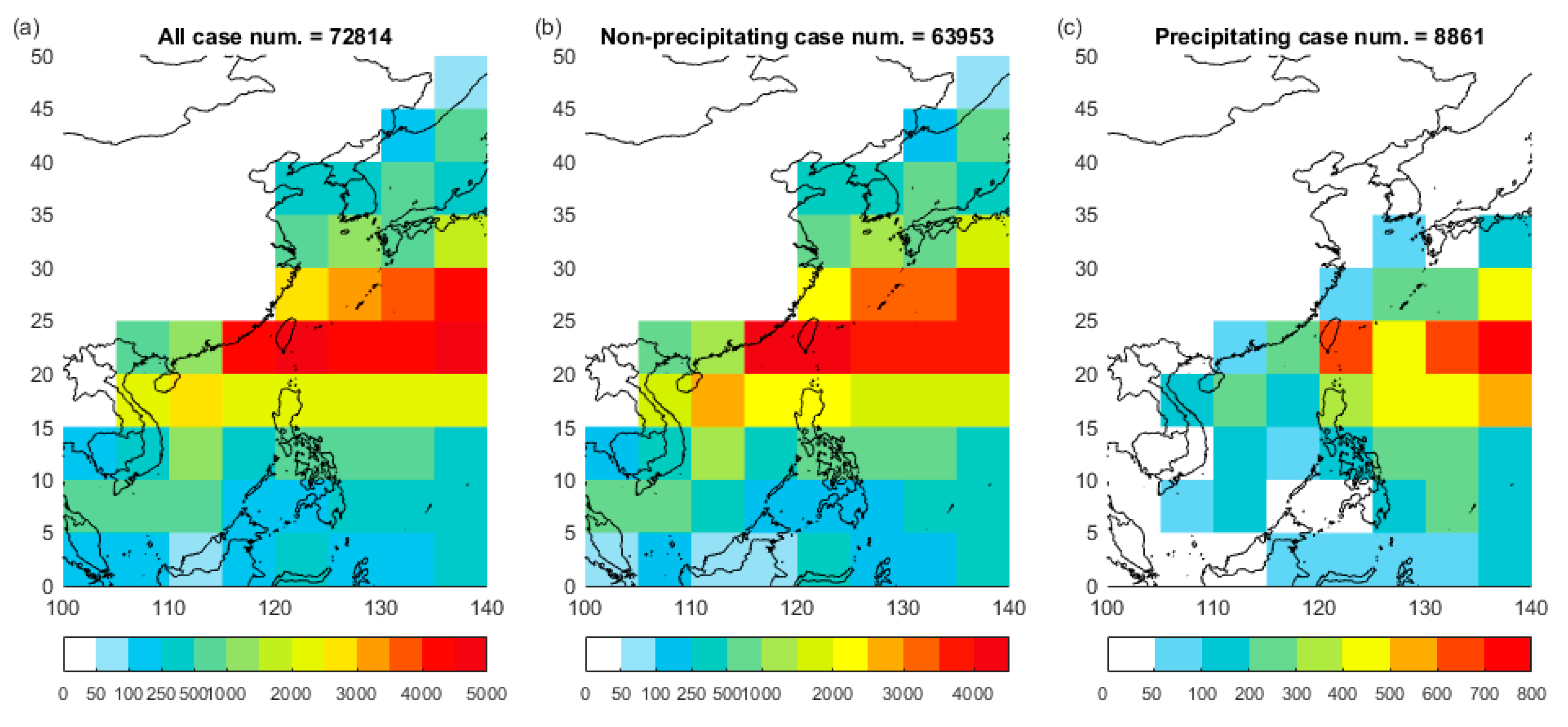
Figure 3 shows the spatial distribution of data sampling for marine warm clouds analyzed in this study. In total, there were 72,814 samples of marine warm clouds in winter (DJF) and spring (MAM) together between the years 2006–2010, mostly detected over the region extended from Taiwan Strait to the East China Sea (20–30
N, 115–140
E,
Figure 3a). There were 49,107 and 23,707 samples in DJF and MAM, respectively. The samples were further separated into the non-precipitating cloud (
Figure 3b) and the precipitating cloud (
Figure 3c); each accounted for 87.8% and 12.2% of the total samples, respectively, with similar spatial patterns.
3. Results
3.1. Spatial Distribution of Environments and Aerosols
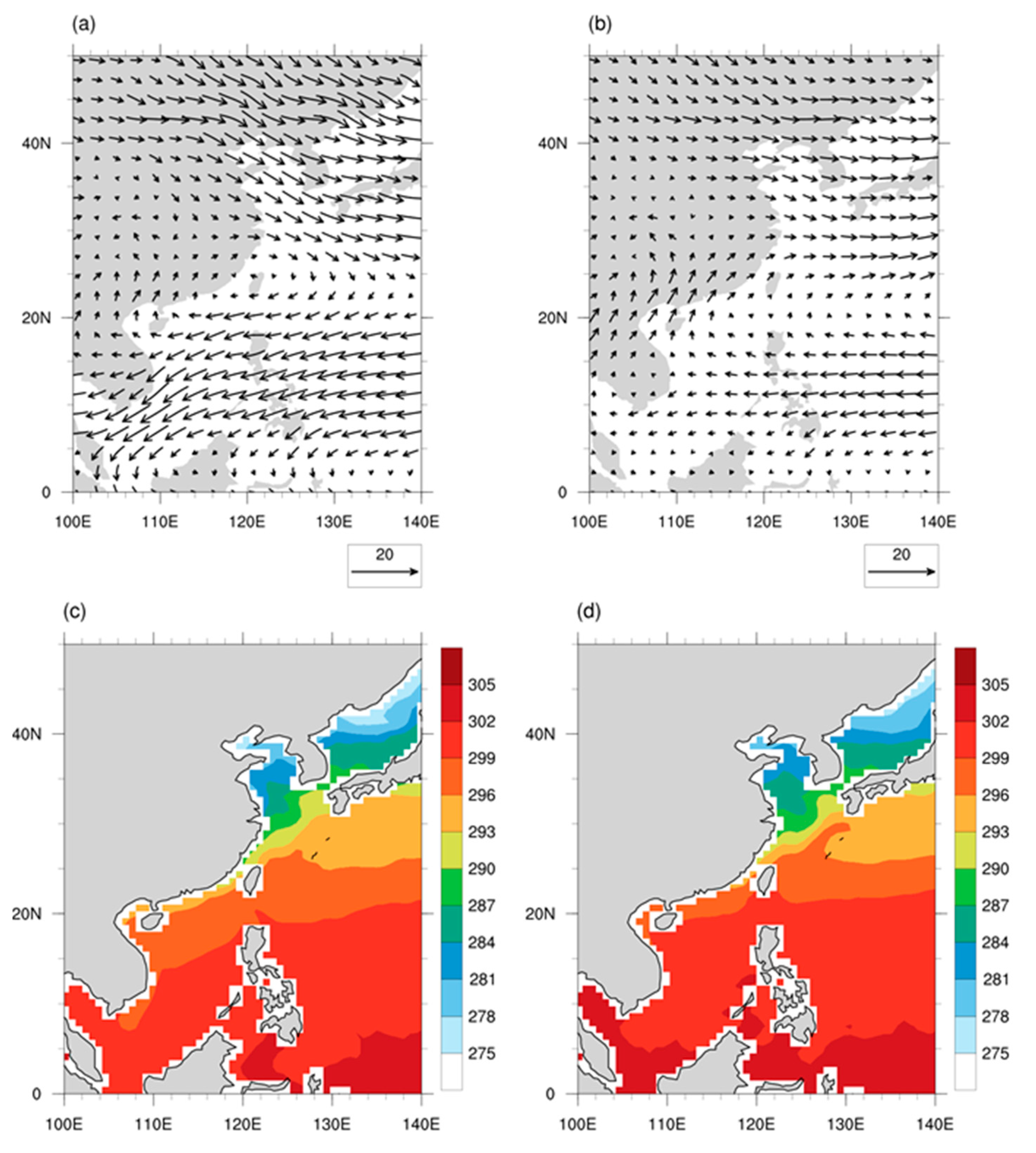
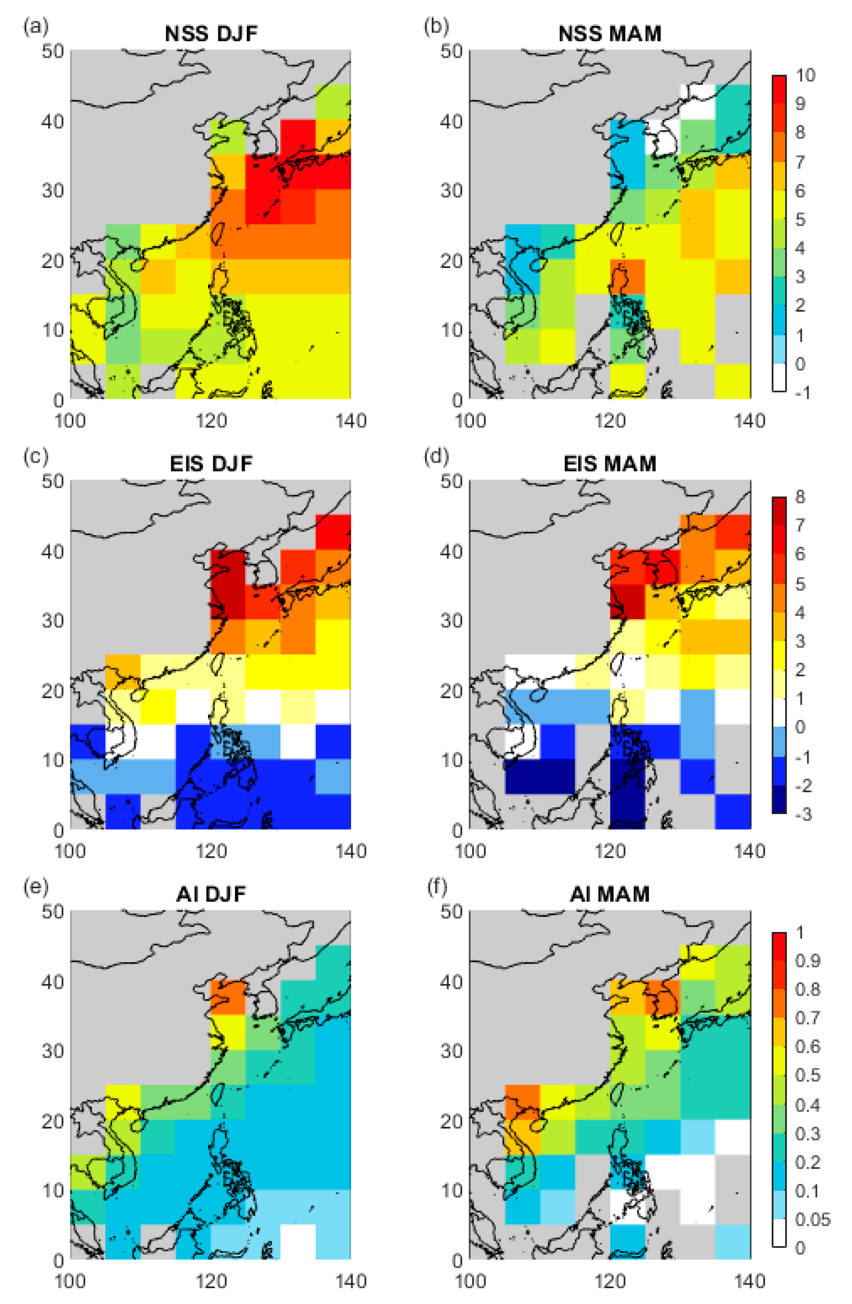
We first examined the seasonal distribution of environmental parameters for marine warm clouds from 2006–2010, including low-level winds, SST, NSS, EIS, and aerosol index. In winter, the horizontal winds at the 850-hPa level showed an anticyclonic flow centered around Taiwan (
Figure 4a). The low-level winds advect cold air from the East Asian continents across the sharp SST gradient over the East China Sea (
Figure 4c), then reach the warm ocean (296–300 K) around 20–30° N, where the Kuroshio transports warm the surface water towards the east coast of Japan. The cold air above the warm ocean corresponds to a thermodynamically unstable marine boundary layer, as represented by the high NSS over 25–35
N and 125–140
E (
Figure 5a), with a maximum value of 11.4 K. The EIS in winter (
Figure 5c), on the other hand, maximizes along the coastal ocean of East China and gradually decreases eastward and southward, following the intensity gradient of large-scale subsidence along the edge of the continental high-pressure system. The low-level winds also transported the anthropogenic aerosols from the major emission sources in northeastern China to the clean marine environment, creating a sharp gradient in the aerosol index (
Figure 5e) decreasing from the Yellow Sea downwind to the East China Sea.
In spring, the low-level winds south of 25° N turn southwesterly, confluent with the northwesterly winds around 30° N (
Figure 4b). The warm SST belt southwest of Japan becomes narrower in spring (
Figure 4d), while the SST gradient remains strong along the continental coast. The weaker cold advection and the more restricted area of warm SST led to a less significant air–sea temperature gradient and, hence, the much lower NSS in springtime (
Figure 5b). The EIS also decreases (
Figure 4d) as the subsidence from the continental high is weakened. The aerosol index over the ocean in spring (
Figure 5f) is generally higher than in winter, yet spatially more homogeneous. Part of the signal is likely contributed by the more active long-range transport of dust particles during spring.
3.2. Aersol and Cloud Properties under Different Regimes
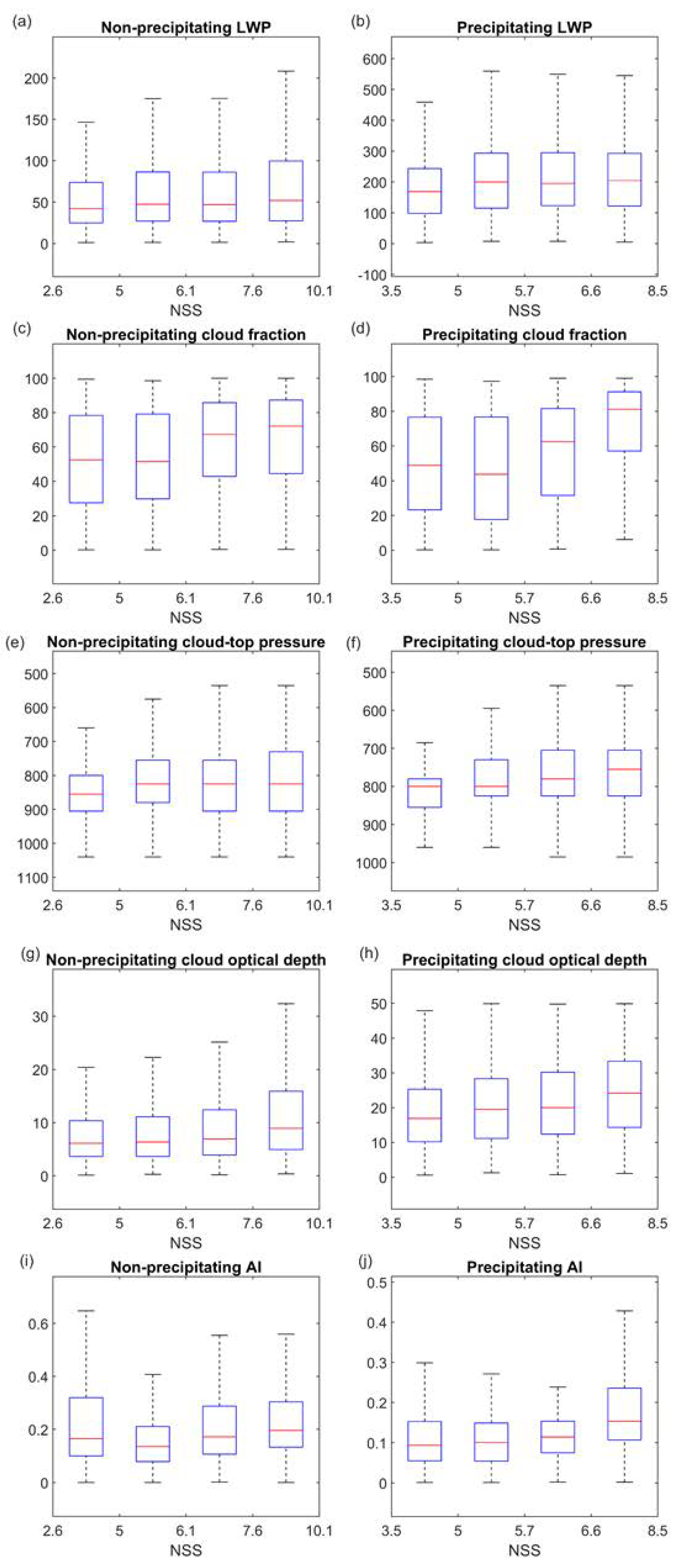
The distribution of LWP, cloud fraction, cloud-top pressure, and cloud optical depth of non-precipitating and precipitating clouds within each NSS interval (10th–30th, 30th–50th, 50th–70th, and 70th–90th percentiles) is shown in
Figure 6a–h.
As NSS increased, the changes in the cloud properties manifested the transformation from stratiform clouds to cumulus clouds. For both non-precipitating and precipitating clouds, the LWP, cloud fraction, cloud-top pressure, and cloud optical depth increased as the NSS increased.
For the non-precipitating clouds, in the most stable interval (NSS = 2.6 K − 5.0 K), 25th percentile (Q1) and 75th percentile (Q3) of LWP were 24.9 and 73.7 g m−2; Q1 and Q3 of the cloud fraction were 27.6% and 78.3%; Q1 and Q3 of cloud-top pressure were 800 hPa and 905 hPa; and Q1 and Q3 of the cloud optical depth were 3.6 and 10.4. In the most unstable interval (NSS = 7.6 K − 10.1 K), Q1 and Q3 of LWP were 27.4 and 99.8 g m−2; Q1 and Q3 of the cloud fraction were 44.5% and 87.3%; Q1 and Q3 of cloud-top pressure were 730 hPa and 905 hPa; and Q1 and Q3 of the cloud optical depth were 4.9 and 15.9. The values of the cloud properties increased with NSS.
For the precipitating clouds, in the most stable interval (NSS = 3.5 K − 5.0 K), the Q1 and Q3 of LWP were 98.4 and 243.3 g m−2; Q1 and Q3 of the cloud fraction were 23.3% and 76.6%; Q1 and Q3 of the cloud-top pressure were 855 hPa and 780 hPa; Q1 and Q3 of the cloud optical depth were 10.2 and 25.3. In the most unstable interval (NSS = 6.6 K − 8.5 K), Q1 and Q3 of LWP were 122.1 and 292.6 g m−2; Q1 and Q3 of the cloud fraction were 57.1% and 91.3%; Q1 and Q3 of cloud-top pressure were 825 hPa and 705 hPa; and Q1 and Q3 of the cloud optical depth were 14.3 and 33.4.
As the NSS increased, the marine boundary layer became more unstable and enhanced the updrafts within the marine boundary layer, which is favorable to the occurrence of shallow convection and leads to the transformation of the stratiform clouds to cumuli.
The distribution of AI in each NSS interval is shown in
Figure 6i,j. For non-precipitating pixels, AI was higher under the lowest NSS condition (Q
1 and Q
3 of AI were 0.1 and 0.3, respectively), representing the nearshore environment in the spring where the marine boundary layer is stable and the aerosol concentration is high. Except for the nearshore condition, AI increased with NSS in both non-precipitating and precipitating conditions. NSS was controlled mainly by the temperature near the surface since the variation in SST was relatively small. As the continental cold air moved over the relatively warm ocean, it not only destabilized the marine boundary layer but brought more aerosol particles to the open ocean, which can be seen in the distribution of AI in all the NSS intervals.
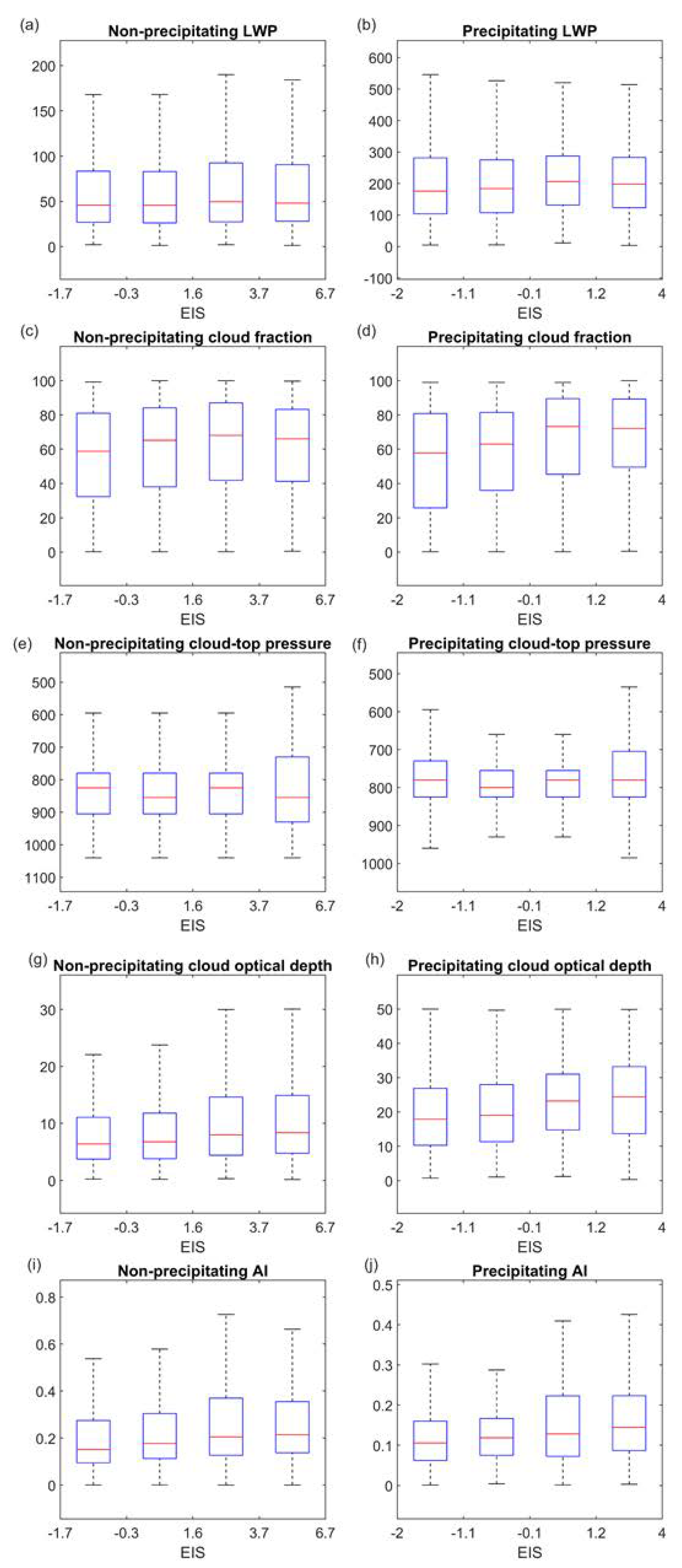
The distribution of LWP, cloud fraction, cloud-top pressure, and cloud optical depth of non-precipitating and precipitating clouds in each EIS interval (10th–30th, 30th–50th, 50th–70th, and 70th–90th percentiles) is shown in
Figure 7a–h. As the EIS increased, the LWP, cloud fraction, and cloud optical depth of the non-precipitating clouds increased, while there was no increasing trend in the cloud-top pressure. The change in cloud properties of precipitating clouds to increasing EIS was similar to that of non-precipitating clouds. As the continental high pressure moved outward, the strong subsidence inhibited the activity of shallow convection and the cloud-top height, while the LWP, cloud fraction, and cloud optical depth increased with EIS, indicating that the cloud-type was primarily the stratiform rather than cumuli.
The distribution of AI in each EIS interval is shown in
Figure 7i,j. For non-precipitating pixels, AI was higher when EIS was strong, and the precipitating pixels also exhibited similar distribution. This suggests that the aerosols tended to accumulate in the boundary layer as the large-scale subsidence strengthened.
3.3. Cloud Susceptibility to Aerosols
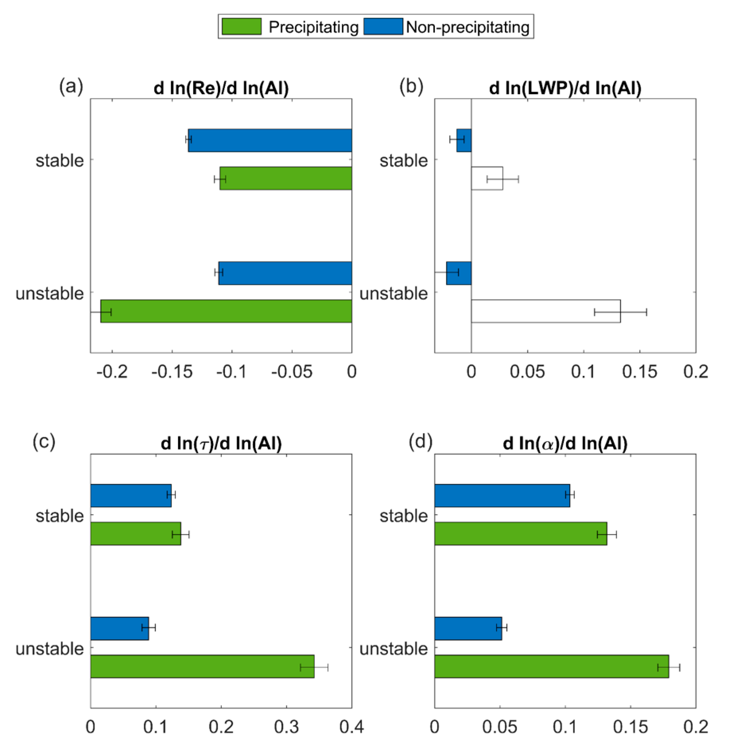
The relatively stable and unstable boundary layer was defined as NSS < 25th percentile and NSS > 75th percentile, respectively, for non-precipitating and precipitating clouds. The sensitivities of cloud properties to aerosols under stable/unstable marine boundary layer are shown in
Figure 8. Consistent with the Twomey effect, the cloud effective radius decreased with AI (
Figure 8a). For non-precipitating clouds, Re was more sensitive to AI under stable boundary layer, as higher stability was associated with less moisture flux from the ocean and, thus, more change in droplet size under higher AI. Note that for precipitating clouds, the sensitivity of Re to AI may have been subject to aerosol removal by precipitation, making it more complicated to analyze.
Under both stable and unstable conditions, LWP decreased with AI for non-precipitating clouds and increased with AI for precipitating clouds (but not statistically significantly) (
Figure 8b). For non-precipitating clouds, the increased aerosols led to smaller cloud droplets, which were more likely to evaporate due to the evaporation-entrainment feedback, resulting in cloud water depletion and, thus, lower LWP. The difference in LWP sensitivity between low and high NSS was not significant for non-precipitating clouds. For precipitating clouds, on the contrary, the suppressed precipitation under polluted conditions led to enhanced LWP. Under the unstable boundary layer, the LWP for precipitating clouds increased with AI due to more moisture supply from the ocean.
The sensitivity of cloud optical depth and cloud albedo to AI were positive under different stability conditions (
Figure 8c,d). Under the unstable condition, the cloud optical depth and cloud albedo for precipitating clouds revealed higher sensitivity to AI than that under the stable condition. With increased AI, the suppressed precipitation resulted in less evaporative cooling below the cloud, enhancing the turbulent mixing within the boundary layer and providing more moisture from the ocean surface. This further led to higher LWP, higher cloud optical depth, and cloud albedo under the unstable environment, consistent with the finding in Chen et al. [
12].
For non-precipitating clouds, the sensitivity of cloud optical depth and cloud albedo to AI was lower under unstable condition than that under stable condition, which was contrary to precipitating clouds. Under the unstable boundary layer, the enhanced turbulence with increased AI led to further entrainment drying for non-precipitating clouds. This resulted in lower LWP response, lower cloud optical depth, and cloud albedo response to AI (
Figure 8b–d).
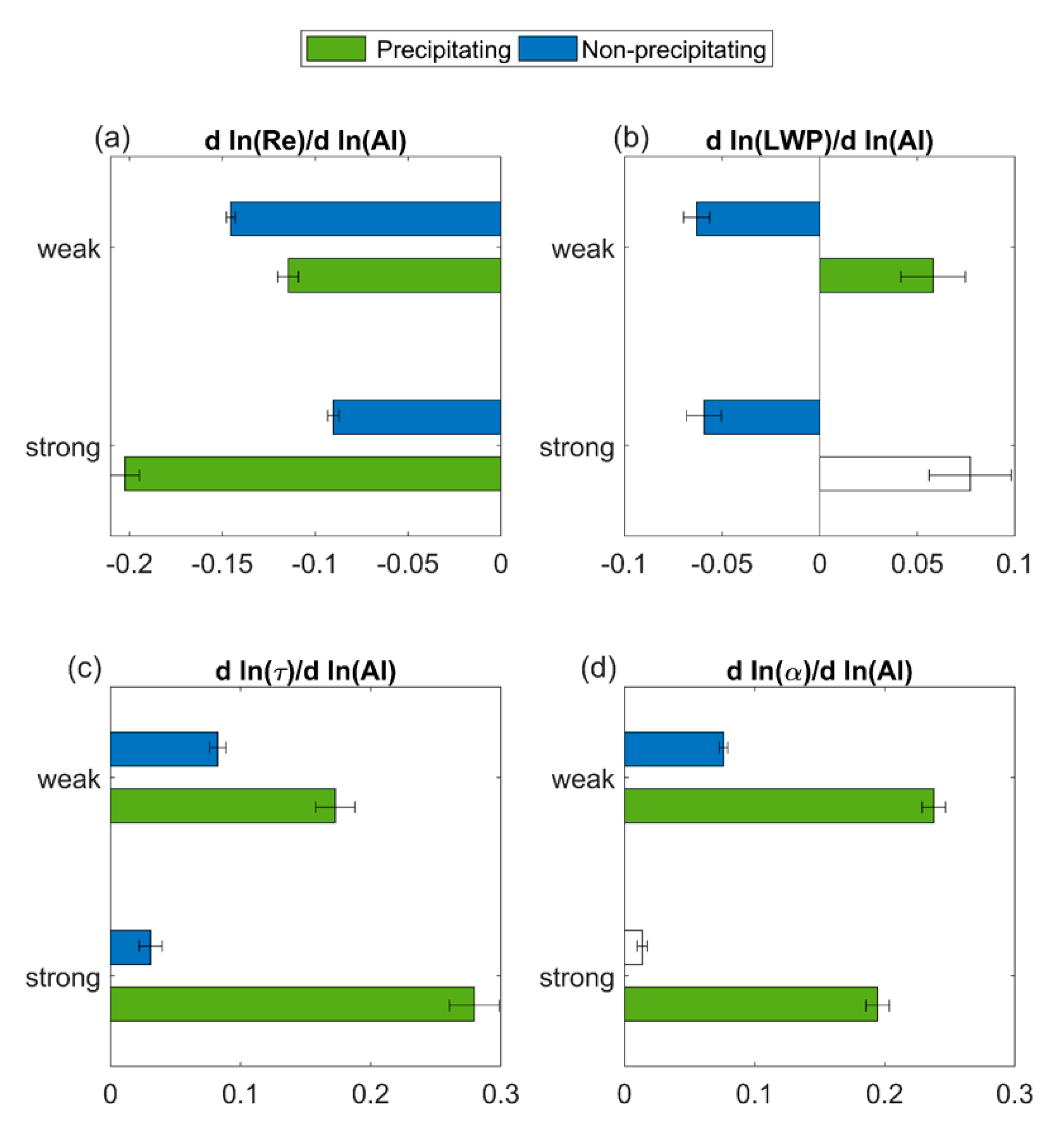
The threshold value for weaker and stronger inversion was defined as EIS < 25th percentile and EIS > 75th percentile, respectively. The sensitivities of cloud properties to AI under weak/strong inversion strength are shown in
Figure 9. The cloud effective radius decreased with increased AI under different inversion strengths (
Figure 9a). For precipitating clouds, the sensitivity of Re to AI may have been associated with aerosol removal by precipitation, which was challenging to investigate directly.
The sensitivity of LWP to AI was negative for non-precipitating clouds and positive for precipitating clouds (
Figure 9b). As previously discussed, for non-precipitating clouds, the enhanced entrainment drying under the polluted condition led to lower LWP, whereas the suppressed precipitation resulted in higher LWP for precipitating clouds. The difference in LWP sensitivity between weak and strong inversion strengths was not significant.
The cloud optical depth and cloud albedo revealed higher susceptibility to increased AI for precipitating clouds than non-precipitating clouds, as shown in
Figure 9c,d. Under stronger inversion, the cloud albedo susceptibility for these clouds was lower than that under weaker inversion, revealing that with stronger entrainment drying, the cloud albedo response to increased AI declined.
4. Discussion
The sensitivity of marine warm cloud properties to AI was higher for precipitating clouds than that for non-precipitating clouds over East Asia. In general, cloud LWP for precipitating clouds was higher than non-precipitating clouds, as shown in
Figure 5a,b and
Figure 6a,b. Therefore, the separation of precipitating and non-precipitating clouds was somewhat equivalent to the separation of clouds with higher and lower LWP. Under higher LWP, the cloud droplets were more likely to grow into drizzle via the collision-coalescence process. In this stage, increased aerosol would suppress the drizzle, resulting in increased LWP. Under lower LWP, on the other hand, there was barely drizzle formation in the clouds as collision-coalescence was not the major process. The smaller cloud droplets under higher aerosol levels were more likely to evaporate via evaporation-entrainment feedback, leading to lower LWP.
In this study, we compared the aerosol–cloud interactions under “relatively stable versus unstable boundary layer” and “weaker versus stronger inversion. The actual values of the environmental parameters were not the focus of our analysis. By choosing the threshold of <25th percentile and >75th percentile for each cloud group, the cloud pixel number for each regime was distributed equally and sufficiently statistically. It is worth noting that, despite the separation method (e.g., separation based on all clouds), the trend of susceptibility remained the same for different environmental regimes and cloud statuses.
Over the global ocean, the main regions dominated by marine stratocumulus clouds are located in the Northeast Pacific, Southeast Pacific, and Southeast Atlantic (i.e., the subtropical oceans near the west coasts of continents, in the descending branch of the Hadley cell). The major environmental factors affecting the aerosol–cloud interactions are not quite the same for typical marine warm cloud regions and the East Asian oceanic regions. In earlier studies (e.g., [
10,
12]), LTS and RH
ft were the key environmental factors in affecting the aerosol–cloud interactions for global marine warm clouds. We also analyzed LTS and RH
ft in this study. We found that LTS tended to overestimate the stability over East Asia. Besides, the aerosol–cloud interaction was not sensitive to change in RH
ft due to the overall high relative humidity over East Asia. Here, we identified that NSS and EIS are major factors influencing the East Asian marine warm cloud responses to aerosols. This revealed that the environmental parameters governing the aerosol–cloud interactions may vary for different regions, depending on the thermodynamic state.
5. Conclusions
During winter and spring, East Asia is mainly influenced by the winter monsoon, under which low-level warm clouds frequently form over the ocean, and the anthropogenic aerosols over land are transported to the ocean via monsoon circulation. Based on our analysis, major meteorological factors affecting the East Asian marine warm clouds and aerosol–cloud interactions include NSS (controlled by the temperature difference between the air and ocean surface) and EIS (influenced by large-scale subsidence). In this study, we selected the A-Train co-located aerosol and oceanic warm cloud data from 2006 to 2010 winter and spring over East Asia, characterized the aerosol and warm cloud properties under different NSS/EIS regimes, and investigated the sensitivities of warm cloud properties to increased AI under different environmental scenarios.
Overall, precipitating clouds reveal higher cloud albedo sensitivity to aerosols as compared to non-precipitating clouds. The cloud LWP increases with aerosol for precipitating clouds, yet decreases with aerosol for non-precipitating clouds, regardless of the environmental regimes. The results are consistent with Chen et al. (2014).
Under the unstable marine boundary layer, there tends to be more turbulent mixing within the boundary layer, leading to more moisture supply from the ocean surface and/or more entrained air near the cloud top. For precipitating clouds, the cloud sensitivity to aerosols is higher under an unstable condition. The LWP increases with AI due to precipitation suppression, and the unstable air further facilitates higher LWP due to more moisture flux from the ocean. Therefore, the cloud optical depth and cloud albedo also reveal higher sensitivity to AI for precipitating clouds under the unstable boundary layer.
The estimated inversion strength is affected by the large-scale subsidence. A weaker inversion strength indicates weaker entrainment from the top of the boundary layer and vice versa. The cloud albedo response to aerosol is lower under stronger EIS than under weaker EIS, showing that stronger EIS weakens the cloud sensitivity due to more pronounced entrainment drying.
Our analysis found NSS and EIS are major factors influencing the marine warm cloud responses to aerosols over East Asia. During spring and winter, the East Asian marine boundary layer is affected by large-scale subsidence from cold high pressure and influenced by the air–sea temperature difference between winter monsoon and Kuroshio current. Our study suggests that the critical environmental parameters governing the aerosol–cloud interactions may vary from region to region. To identify the main factors controlling the cloud responses to aerosols, the thermodynamic conditions of the target area need to be well understood.


