Article

Effects of Training Set Size on Supervised Machine-Learning Land-Cover Classification of Large-Area High-Resolution Remotely Sensed Data

by
Christopher A. Ramezan
1,*,
Timothy A. Warner
2,
Aaron E. Maxwell
2 and
Bradley S. Price
1
1
Department of Management Information Systems, West Virginia University, Morgantown, WV 26506, USA
2
Department of Geology and Geography, West Virginia University, Morgantown, WV 26506, USA
*
Author to whom correspondence should be addressed.
Submission received: 28 December 2020 / Revised: 16 January 2021 / Accepted: 18 January 2021 / Published: 21 January 2021
(This article belongs to the Special Issue Remote Sensing Data and Classification Algorithms)

Abstract

:
The size of the training data set is a major determinant of classification accuracy. Nevertheless, the collection of a large training data set for supervised classifiers can be a challenge, especially for studies covering a large area, which may be typical of many real-world applied projects. This work investigates how variations in training set size, ranging from a large sample size (n = 10,000) to a very small sample size (n = 40), affect the performance of six supervised machine-learning algorithms applied to classify large-area high-spatial-resolution (HR) (1–5 m) remotely sensed data within the context of a geographic object-based image analysis (GEOBIA) approach. GEOBIA, in which adjacent similar pixels are grouped into image-objects that form the unit of the classification, offers the potential benefit of allowing multiple additional variables, such as measures of object geometry and texture, thus increasing the dimensionality of the classification input data. The six supervised machine-learning algorithms are support vector machines (SVM), random forests (RF), k-nearest neighbors (k-NN), single-layer perceptron neural networks (NEU), learning vector quantization (LVQ), and gradient-boosted trees (GBM). RF, the algorithm with the highest overall accuracy, was notable for its negligible decrease in overall accuracy, 1.0%, when training sample size decreased from 10,000 to 315 samples. GBM provided similar overall accuracy to RF; however, the algorithm was very expensive in terms of training time and computational resources, especially with large training sets. In contrast to RF and GBM, NEU, and SVM were particularly sensitive to decreasing sample size, with NEU classifications generally producing overall accuracies that were on average slightly higher than SVM classifications for larger sample sizes, but lower than SVM for the smallest sample sizes. NEU however required a longer processing time. The k-NN classifier saw less of a drop in overall accuracy than NEU and SVM as training set size decreased; however, the overall accuracies of k-NN were typically less than RF, NEU, and SVM classifiers. LVQ generally had the lowest overall accuracy of all six methods, but was relatively insensitive to sample size, down to the smallest sample sizes. Overall, due to its relatively high accuracy with small training sample sets, and minimal variations in overall accuracy between very large and small sample sets, as well as relatively short processing time, RF was a good classifier for large-area land-cover classifications of HR remotely sensed data, especially when training data are scarce. However, as performance of different supervised classifiers varies in response to training set size, investigating multiple classification algorithms is recommended to achieve optimal accuracy for a project.

1. Introduction

One of the key determinants of classification accuracy is the training sample size [1], with larger training sets typically resulting in superior performance compared to smaller training sets. However, in applied remote sensing analyses, training data may be limited and expensive to obtain, especially if field observations are needed. In circumstances where the number of training data is limited, or where constraints in processing power or time limit the number of training samples that can be processed, it would be advantageous to know the relative dependence of machine-learning classifiers on sample size. For example, an analyst may want to know the potential for increased classification accuracy if additional resources were invested in increasing the number of training samples. Alternatively, if a very large sample size is available, does this potentially affect the classifier choice?
The existing literature on training sample size and its effect on classification accuracy offers only partial insight into these questions. Most previous studies comparing supervised machine-learning classifier accuracy have used a single, fixed training sample size [2,3,4], and thus have ignored the effects of variation in sample size. Conversely, investigations that have examined the effects of sample size, for example [1,5,6], have generally focused on a single classifier, making it difficult to compare the relative dependence of machine-learning classifiers on sample size.
The small number of studies that have investigated varying training set size on multiple supervised classifiers have generally considered only a narrow range in sample sizes, and often focused on other characteristics of the training set, such as class imbalance [7,8] or feature set dimensionality [9]. For example, an important study by Myburgh and Niekerk [9] investigated the effects of sample size on four machine-learning classifiers. However, their experiment explored only a small range of sample sizes, 25–200, and those samples were collected from a relatively limited urban study area. Furthermore, although they included classification and regression tree (CART) classification, they did not include the popular random forest classifier. Another study, Qian et al. [10] also examined the effects of training set size on various supervised classifiers in a geographic object-based image analysis (GEOBIA) classification. However, Qian et al. [10] examined a narrow range of sample sizes, 5–50 samples per class. They also conducted their investigation using Landsat-8 OLI imagery, a medium spatial resolution dataset, which was applied to a single district within Beijing. Furthermore, their study, similar to that of [9], did not include either neural networks or k-nearest neighbors classifiers.
This paper therefore furthers the investigation into the effects of sample size on supervised classifiers by examining a broad range of training sample sizes, ranging from a large sample size of 10,000, with each class having a minimum of 1000 samples, to a very small training sample size of 40, where certain classes may have as few as 4 training samples. The effect of sample size is compared for six supervised machine-learning classifiers, support vector machines (SVM), random forests (RF), k-nearest neighbors (k-NN), single-layer perceptron neural networks (NEU), learning vector quantization (LVQ), and gradient-boosted trees (GBM). SVM, RF, k-NN, NEU, and GBM classifiers are commonly implemented in remote sensing analyses [11], with combinations of these classification algorithms used in comparative analyses of classifier performance on remotely sensed data [2,12,13]. LVQ was also selected for this analysis, as it is used in a variety of other fields such as accounting [14], mechanical engineering [15], and medical imaging [16], but as yet has rarely been used to classify remotely sensed data. The accuracy of the classifications is evaluated with a large, independent validation sample set.
As most previous investigations comparing supervised machine-learning classifier dependence on sample size have employed relatively small test areas, this analysis examines classifier response to varying training sample sizes when applied to classify a high-spatial-resolution (HR, 1–5 m) remotely sensed dataset covering a large area. A GEOBIA approach is used because GEOBIA has been found to be particularly effective for classifying HR remotely sensed data [17,18]. GEOBIA is a relatively new paradigm in remote sensing which has become increasingly popular in both theoretical and applied analyses in recent years. GEOBIA applies image segmentation techniques to group similar pixels into discrete, non-overlapping image-objects. Unlike pixel-based data which are uniform in size and shape, GEOBIA image-objects can provide potentially useful geometric information which may serve as additional predictor variables for classification methods. Furthermore, GEOBIA image segmentation approaches have proven particularly useful for reducing the salt-and-pepper noise effect experienced in pixel-based analyses of high-resolution remotely sensed data [18]. The remotely sensed data used comprises 4-band color infrared 1 m United States National Agriculture Imagery Program (NAIP) orthoimagery, combined with 1 m light detection and ranging (LIDAR)-derived normalized digital surface model (nDSM) and intensity raster grids.

2. Materials and Methods

2.1. Study Area and Remotely Sensed Data

The study site is in the state of West Virginia, USA, between latitudes 79°55′ W and 79°30′ W and longitudes 39°42′ N and 39°0′ N, encompassing a multi-county area including Preston County, and portions of Monongalia, Taylor, Barbour, and Tucker counties (Figure 1). The total size of the study area is 260,975 ha, which is 4.2% of the area of the entire state of West Virginia. The terrain is mountainous, with elevations of 548–914 m, and mostly forested.
Two types of remotely sensed data were used: passive optical multispectral imagery, and a LIDAR point cloud (Figure 1). The optical dataset comprises four-band color infrared leaf-on NAIP orthoimagery [19]. The spectral bands of the NAIP imagery include blue (400–580 nm), green (500–650 nm), red (590–675 nm), and near-infrared (NIR) (675–850 nm). The imagery has 1 m spatial resolution and 8-bit radiometric resolution. The NAIP data were acquired via a series of aerial flights between 17 July and 30 July 2011. A small portion of the NAIP imagery within the study area, less than 3% of the total, was collected on 10 October 2011. The NAIP imagery were provided as 108 individual uncompressed digital orthophoto quarter quadrangles (DOQQs) in a tagged image file format (.tiff).
The LIDAR data were acquired between 28 March and 28 April 2011, using an Optech ALTM-3100C sensor [20] with a 36° field of view and a pulse frequency of 70,000 Hz. The LIDAR data were provided as 1164 individual LASer (.las) files, containing a combined total of 5.6 × 10⁹ points. The LIDAR point cloud data include elevation, intensity, up to four returns, and a basic classification of the points provided by the vendor. A pilot investigation determined there was minimal change in the land cover during the approximately four months between the acquisition dates of most of the LIDAR and NAIP data.
This study site was chosen as it contained a diverse set of landforms including forests, rivers, lakes, mountains, valleys, urban and suburban developed areas, and croplands, as well as anthropogenic landforms such as mines, at a variety of elevations. The boundary of the study area was largely defined by the extent of the LIDAR point cloud. Four land-cover classes were mapped for this analysis: forest, grassland, soil and water (Table 1).

2.2. Data Processing and Image Segmentation

The LIDAR tiles first were combined into a single large LIDAR point cloud stored as a LASer (LAS) dataset. Elevation and intensity information in the LIDAR point cloud were used to develop a normalized digital surface model (nDSM) and an intensity raster, respectively. LIDAR-derived elevation and intensity surfaces have been demonstrated to improve the accuracy of land-cover classifications of HR multispectral imagery, especially if the spectral resolution of the imagery is low [21].
The LAS to Raster function in ArcMap 10.5.1 [22] was used to rasterize the LIDAR point cloud. Elevation data in the LIDAR point cloud were used to first develop a bare earth digital elevation model (DEM) and a digital surface model from the ground and first returns, respectively. An nDSM was produced by subtracting the DEM from the DSM.
The intensity of the first returns in the LIDAR point cloud was rasterized to generate an intensity surface using the ArcMap LAS to Raster function. A binning approach was used to determine cell values. Cell values were assigned the average value of all points contained within each cell. Linear interpolation was used to determine cell values for any voids contained within the point cloud. Slant range distance was not available, and thus it was not possible to correct for beam spreading loss or other factors. Previous research has shown that even in the absence of calibration of LIDAR intensity, LIDAR intensity data are useful for land-cover classification [23]. The pixel size of both the nDSM and LIDAR intensity raster grids was set to 1 m, matching the pixel size of the NAIP orthoimagery. A 5 × 5-pixel median filter was applied to the LIDAR raster grids, to remove artefacts likely caused by the “sawtooth” scanning pattern of the OPTECH ALTM 3100 sensor and the 1 m rasterization process [24].
The NAIP tiles were mosaicked and color-balanced into a single large image using the Mosaic Pro tool in Earth Resources Data Analysis System (ERDAS) Imagine 2014. As NAIP imagery comprise multiple flight lines of data acquired at different times of the day [19], radiometric variation can occur between NAIP tiles. In large-area analyses of NAIP data, this can be a particular concern, as a larger study area is likely to include more radiometric variation. Thus, color-balancing was applied during the mosaic process to reduce radiometric variation between the NAIP orthoimagery tiles [25]. The NAIP orthomosaic was then clipped to the boundaries of the LIDAR raster grids. The NAIP and LIDAR raster grids were combined into a single, six-layer stack, comprising the four NAIP bands and two LIDAR bands.
Trimble eCognition Developer 9.3 multi-resolution segmentation (MRS) was chosen as the segmentation method for this analysis. MRS is a bottom-up region-growing segmentation approach that partitions images into distinct image-objects [26]. Equal weighting was given to all six bands for the segmentation.
The MRS algorithm has three parameters that require input from the analyst: scale, shape, and compactness [26]. The scale parameter (SP) determines the size of the image-objects, and is usually assumed to be the most important [13,27,28]. The SP value is typically chosen through trial and error [29,30], although that approach has been criticized as ad hoc, not replicable, and not able to guarantee a near-optimal value [31]. The estimation of scale parameter (ESP2) tool, an automated method for SP selection developed by Drăguţ et al. [32], iteratively generates image-objects at multiple scale levels. The tool then plots the rate of change of the local variance (ROC-LV) against the associated SP. Peaks in the ROC-LV curve indicate SPs with segment boundaries that tend to approximate natural and synthetic features [27].
As the ESP2 tool requires a large amount of computing resources, three small areas of the study area were randomly selected to run the ESP2 process. The results suggested SP values of 97, 97, and 104, and therefore an intermediate value, 100, was selected for the MRS segmentation. The default shape and compactness parameters of 0.1 and 0.5 respectively were used, as varying these parameters did not appear to improve the quality of the segmentation. The segmentation of the dataset generated 474,614 image-objects.
Unlike pixels, which are uniform in size and shape, image-objects in object-based image analyses can include not only spectral information, but also spatial information. A total of 33 spectral and geometric predictor variables were generated for each image-object (Table 2). Spectral variables include the mean, mode, standard deviation, and skewness of each image band. In addition, a separate spectral value Brightness was also included. The Brightness value of objects was calculated as the average mean values of the four NAIP bands, over all the pixels in the object [33]. NDVI was calculated using the Red and NIR spectral bands from the NAIP data. Examples of geometric variables include object roundness, border length, and compactness.

2.3. Training Sample Collection

Two separate, large sample sets, each containing 10,000 samples, were collected from across the entire dataset. One large sample set was used as training data while the other large sample set was used as an independent validation set used for testing the classifier accuracies, and was not used in training. As this analysis was conducted in a GEOBIA framework, image-objects were the sampling unit. The class label was assigned by photo-interpretation of the original NAIP imagery. Image-objects were found to almost always represent a single class. In the rare instances that they did not, the majority class within the object was used as the class label.
For convenience, the validation data set (described in the next section) was generated first, and then the training sample set was collected. To ensure the independence of the validation dataset, the image-objects in the validation dataset were removed from the population before collecting the training dataset. As the study area is overwhelmingly dominated by the forest class, the proportions of the classes in the image did not allow for an equalized stratified sampling. Therefore, disproportional stratified random sampling was used for the training data sample collection to ensure adequate representation of extreme minority classes in the training sets. Disproportional stratified random sampling involves the selection of samples from pre-defined strata, where each member of the stratum has an equal probability of being selected, but the size of the strata is defined by the analyst. Previous research has indicated that disproportional stratified random sampling is an effective approach for training data collection in large-area supervised land-cover classifications of HR remotely sensed data where extreme minority classes are present in the study area [34]. Randomly collected training data improves the representativeness of the samples, and the disproportional stratified approach can reduce class imbalance [34]. For this study, the strata sizes were defined as 50% forest, 20% grassland, 20% soil, and 10% water.
The large training sample set (n = 10,000) (Figure 2) was randomly subset into a series of smaller training sets, with each subset independently chosen from the original 10,000, and each successive set approximately half the size of the preceding larger set. This resulted in training sets of size 10,000, 5000, 2500, 1250, 626, 315, 159, 80, 40. Class strata proportions were maintained for each sample set, which explains why each successively smaller sample is not exactly half of the larger set. The smallest training sample used was 40, because a preliminary analysis showed that sample sizes smaller than 40 caused problems with the cross-validation parameter tuning due to the small number of samples in the water class. Table 3 summarizes the training sample sets and the validation dataset.

2.4. Validation Sample Collection

As described in the previous section, the validation data were completely separate from the training data, and were generated prior to the collection of the training data. Simple random sampling was used to select the validation dataset samples [34]. Simple random sampling has the benefit that the population error matrix can be estimated directly from the sample statistics [35]. The size of the validation sample set (n = 10,000) was approximately 2.1% of the total image-objects generated across the entire study area. Image-objects included in the validation sample were manually labeled by the analyst.

2.5. Supervised Classification Methods

Six supervised machine-learning classifiers were compared in this study. The classifications were performed on each training dataset and evaluated against the independent validation dataset. The classifications were performed within R 3.5.1. Table 4 lists the associated R packages. The caret package [36] was used for implementation of the classification methods for all six classifiers.

2.5.1. Support Vector Machines (SVM)

SVM is a non-parametric, supervised machine-learning algorithm that seeks a hyperplane boundary to separate classes [42,43]. A distinctive feature of SVM is that the location of the hyperplane is determined by the training samples closest to the hyperplane, termed support vectors; other training samples are ignored. The optimization maximizes the margin of the hyperplane between the support vectors of the different classes, which is why SVM is sometimes referred to as a maximum margin classifier [44]. As the hyperplane is a linear decision boundary, and many classes are not linearly separable, SVM transforms the feature space to a higher dimension where the data may be linearly separable. This transformation is called the kernel trick. There are a variety of kernel types; we use a radial basis function kernel (RBF), a kernel commonly used in remote sensing [2,43,44,45] and typically employed as a baseline for evaluating the performance of new SVM kernels [46,47]. RBF SVM has two parameters, C, the cost parameter, which trades off misclassification of training examples for maximization of the margin, and σ, which defines the influence of training samples chosen as support vectors on the decision boundary [48]. Higher values of σ typically produce highly curved or flexed decision boundaries, while lower values suggest a more linear decision boundary. In this analysis, optimal values of σ were chosen by the sigest function, which uses a sample of the training set and returns a vector of the 0.1 and 0.9 quantiles of |x − x’|2. The median of the two quantiles is chosen for σ [49].

2.5.2. Random Forest (RF)

RF is an ensemble machine-learning classifier that uses many decision trees, each of which is given random subsets of the training data and predictor variables [50]. The decision trees in the ensemble are produced independently and, unlike typical classification using a single decision tree, are not pruned. After training, each unknown sample is classified based on the majority vote of the ensemble. RF is a commonly used classification method in remote sensing analyses [2,45,51,52,53,54], and has become increasingly popular due to its superior classification accuracies compared to other commonly used classifiers such as single decision trees [54], ease of parameterization and robustness in the presence of noise [55]. Additionally, the RF classifier can be attractive to remote sensing scientists due to its ability to handle high-dimensional datasets [56], an important consideration for hyperspectral [55,57] and object-oriented datasets [58]. The implementation of RF used in this analysis contained 2 parameters, the number of trees, which defines the number of trees in the forest, and mtry which defines the number of variables randomly chosen for splitting at each tree node. In this analysis, the number of trees for all RF classifications was set at 500, a value that is commonly used in remote sensing analyses [59,60,61]. Additionally, two different methods were tested for splitting tree nodes, Gini impurity [62] and the extremely randomized trees method described in [63].

2.5.3. k-Nearest Neighbors (k-NN)

k-NN is a non-parametric classifier, which assigns class membership to new data inputs based upon their proximity to the k closest pre-labeled training data in the feature space. Lower k-values produce more complex decision boundaries, while larger k-values increase generalization [64]. k-NN is often described as a lazy learning classifier because it is not trained; unknowns are compared directly to the training data [65].

2.5.4. Neural Networks (NEU)

NEU classifiers use a series of neurons, organized into layers [66]. All neurons in neighboring layers are connected to each other by matrices of weights. Input layer neurons correspond to predictor variables, while output layer neurons correspond to classes. The neural network is trained by iteratively adjusting the weights to improve the classification, as the training data pass through layers. A feed-forward neural network with a single hidden layer is used in this analysis. Data in this neural network moves only mono-directionally (forward) and uses only one single layer between the input and output layers [39]. An extensive literature on the application of NEU classification in remote sensing has developed over many years [67,68,69]. This implementation of NEU has two parameters; size, which defines the number of units contained within the hidden layer, and decay, which serves as a regularization parameter which helps avoid overfitting [39].

2.5.5. Learning Vector Quantization (LVQ)

LVQ is a classifier that assigns membership to unseen examples using a series of codebook or prototype vectors within the feature space [70]. Codebook vectors are typically randomly selected training data. Training samples in the LVQ algorithm are processed one at a time and are evaluated against the most similar codebook vector in the feature space. If the selected training sample has the same class as the codebook vector, a winner-take-all strategy is pursued, where the “winning” codebook vector is moved closer to the training sample. If the codebook vector does not have the same output as the training sample, the codebook vector is moved further away from the selected training sample in the feature space. This process is repeated until all codebook vectors have been evaluated against all training samples. Once the codebook vectors have been trained, the rest of the training data are discarded. The LVQ classifier predicts unseen examples in a similar manner to k-NN, except the codebook vectors are used for making predictions, rather than the full training data set. Although LVQ is not commonly used in remote sensing analyses (for an exception, see the application of a variant of LVQ in hyperspectral image analysis as described in [71]), it is a widely used classifier in many other fields because of its clear and intuitive learning process and ease of implementation [72]. LVQ has two parameters that can be tuned: size, which influences the number of codebook instances in the model [40], and k-value, the parameter described in Section 2.5.3.

2.5.6. Gradient-Boosted Trees (GBM)

GBM is a tree-based ensemble classifier similar to RF. However, unlike RF, which trains many deep decision trees independently, GBM uses many shallow trees that are built one at a time, sequentially, with the goal of minimizing on errors found from trees built earlier in the training sequence [73,74]. GBM contains four parameters which can be tuned. The number of trees, as with RF, defines the number of decision trees in the ensemble. Interaction.depth specifies the number of splits in each tree. Shrinkage, which can also be seen as the learning rate, defines how quickly the algorithm progresses down the gradient descent. Generally, smaller shrinkage values are thought to improve the predictive performance of the model, but at the cost of increasing training time. n.minobsinnode is the minimum number of observations in the terminal nodes of the trees [41]. Because of its similarity to RF, remotely sensing studies that have compared GBM to other machine-learning methods have generally found it to produce an accuracy that is similar, but slightly lower than, RF (e.g., [75,76], who used a variant called extreme gradient boosting). Methods such as Xgboost [77] have also been developed which expand on GBM from both a methodological and computational perspective by adding regularization parameters to penalize complexity of trees. Xgboost also proposes algorithmic advantages for sparse data and the ability to parallelize the algorithm. We have chosen to implement GBM as it is most similar to RF in the model complexity.

2.6. Cross-Validation Parameter Tuning

Many supervised machine-learning algorithms are parameterized, so they can be optimized for a specific objective or dataset [78,79]. The selection of classifier parameters is an important stage of the classification process. However, as it is normally not possible to predict optimal values for these parameters, empirical cross-validation methods are typically employed [7,34,78,79]. K-fold cross-validation testing was used for parameter tuning [34]. The number of folds was set to 10. Kappa was used to evaluate model parameters instead of overall accuracy, as several cross-validation models reported identical overall accuracy values, but different kappa coefficient values. Table 5 shows the range of parameters values tested for each classifier.

2.7. Classification and Replications

After the optimal parameters for each classification were estimated (Table 6), classifications were conducted for all six machine-learning classifiers (SVM, RF, k-NN, NEU, LVQ, GBM) trained from each of the nine different sets, which varied in sample size (40, 80, 159, 315, 626, 1250, 2500, 5000, 10,000 training samples).
To investigate potential variability in classifier accuracy depending on the composition of the training dataset, each classification was replicated a total of 10 times. New training data sets for sample sizes 40–5000 were simulated by random sub-sampling from the 10,000-sample set using different seed values, resulting in 80 additional training sets (10 for each sample size between 40–5000), which were used to train the iterations of each classifier. Class strata proportions described in Table 3 were maintained in the sub-sampling process. As the 10,000-sample set could not be randomly sub-sampled, the 10 replications for the classifications trained from the 10,000-sample set were trained on the same 10,000 dataset; however, the random seed for the k-fold cross-validation was changed for each iteration, resulting in different folds for each iteration. Thus, because of replication, a total of 540 classifications were run (54 classifications × 10 replications). Each set of 54 classifications within a single replication is referred to as an iteration. Cross-validation parameter tuning was conducted individually for all 540 classifications.
Classifications were run on a custom workstation with an Intel Core i5-6600K Quad-Core Skylake processor with 32.0 GB of GDDR5 memory, and a Samsung 970 EVO NVMe 256 GB M.2. SSD running Windows 10 Pro. Processing time for all classifications were recorded using the rbenchmark package [80]. The processing time statistics should be evaluated in terms of their relative, and not absolute values, as processing time is highly dependent on a variety of factors such as system architecture, CPU allocation, memory availability, background system processes, among other factors. In addition, it is important to note that time taken for training and optimization as well as classification is not just dependent on the number of training samples, the focus of this paper, but also other factors such as the particular implementation of the algorithm, the number of classes, the number of spectral bands, and in the case of the classification, the size of imagery. We also note that the processing time statistics and model accuracies are also representative of our specific implementation within R. Although other software frameworks, programming languages, and code structures may perform differently regarding both accuracy and processing time, these results provide reference of standard implementations using the popularly used R framework. Nevertheless, it is important to note that in particular, the computational times reported in this paper should not be regarded as definitive for other data sets and other implementations of these algorithms. However, the relative processing time of the different experiments is useful for exploring characteristics of the different classifiers.

2.8. Error Assessment

The classifications were evaluated against the large randomly sampled validation dataset consisting of 10,000 image-objects. Results for each classification were reported in a confusion matrix. Overall map accuracy as well as user’s and producer’s accuracies were calculated, as well as the kappa coefficient. Overall accuracy was calculated by the summation of the correctly classified image-objects for each class, divided by the total number of image-objects in the validation dataset. Overall accuracies for all 540 classifications are listed in Appendix A.

3. Results

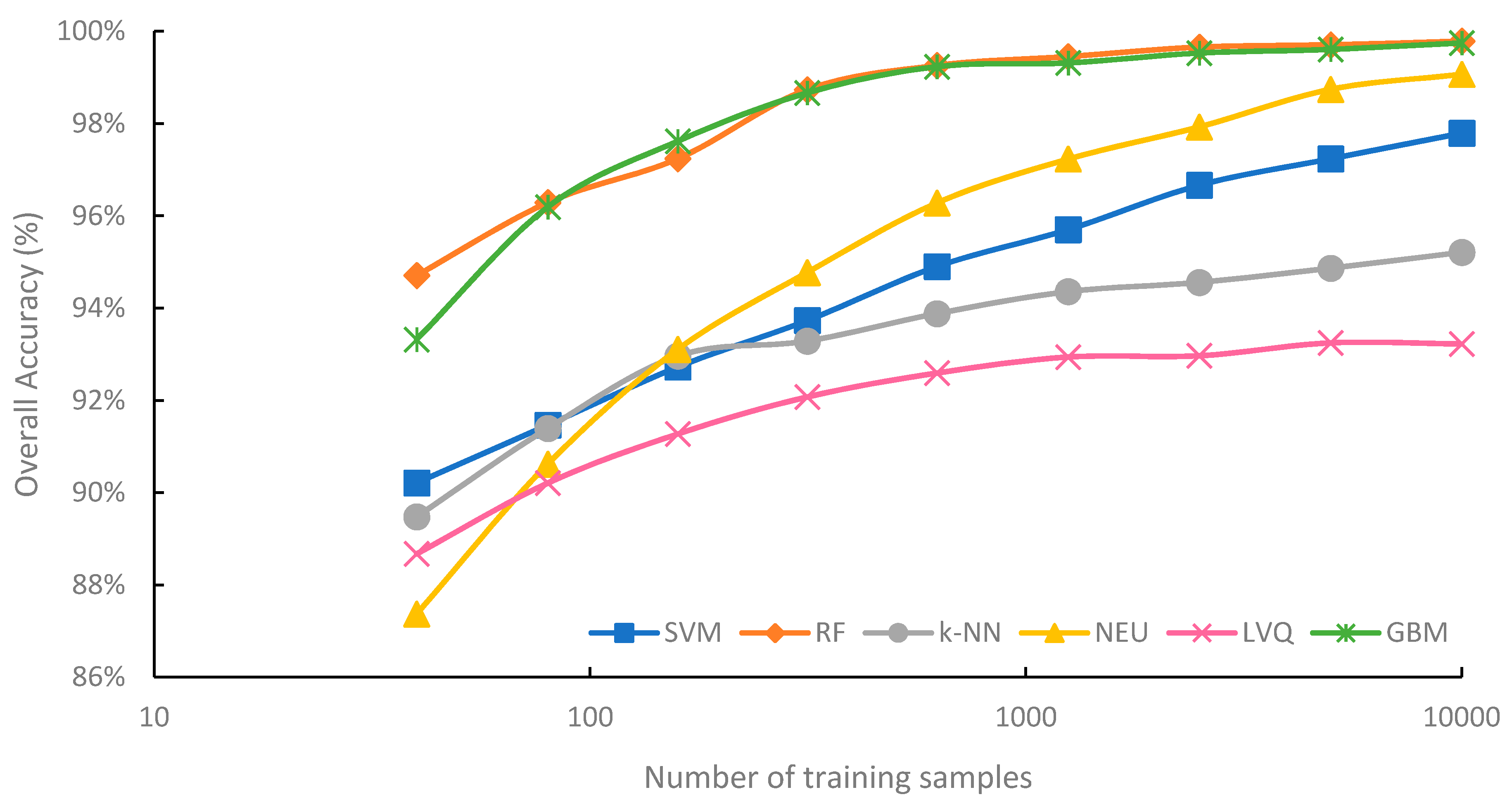
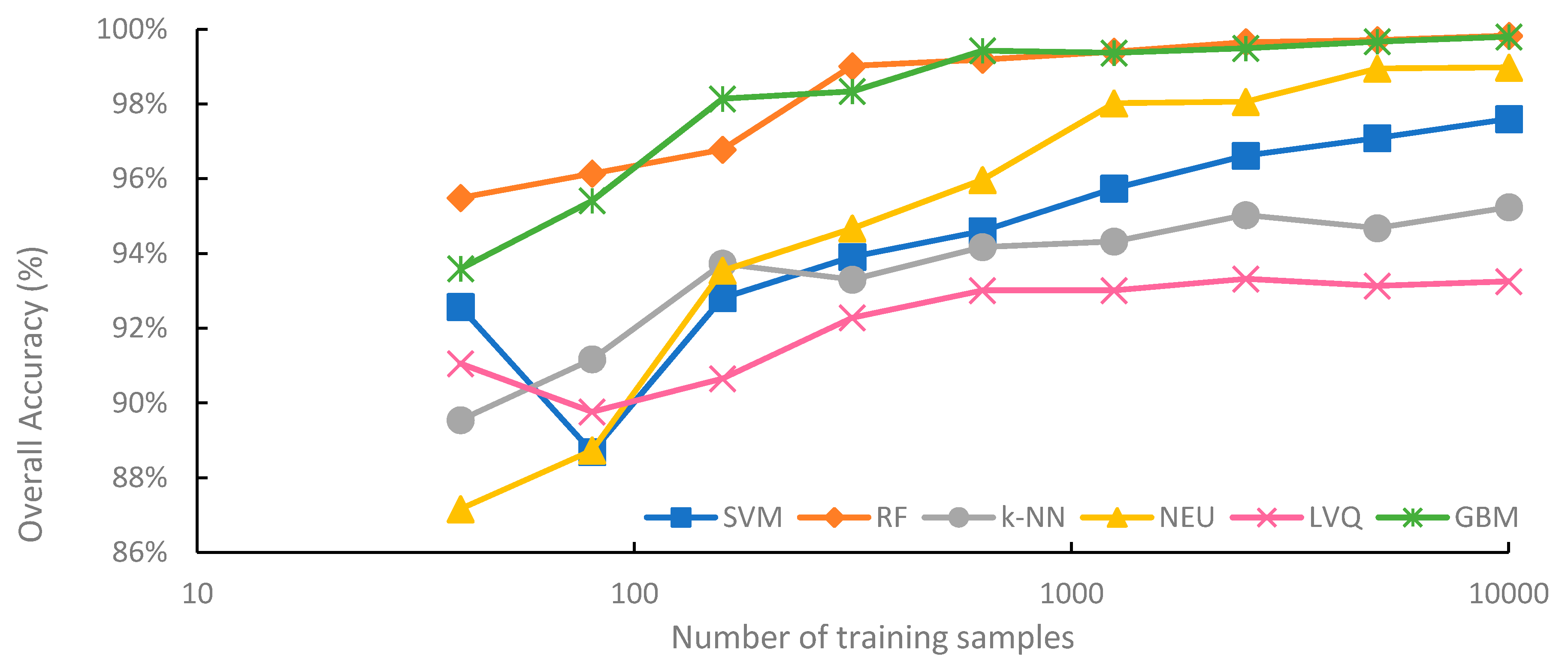
3.1. Accuracy Evaluation

Figure 3 summarizes the mean overall accuracy of the six classification methods evaluated, based on sample size. Generally, overall accuracy increased with sample size. For all classification methods, highest average overall accuracy was produced from the 10,000-sample set, while the lowest average overall accuracy was produced from the 40-sample set. However, each classifier responded to increasing sample size differently. The highest average overall accuracy was 99.8%, for the RF classifications trained from the 10,000-sample set, while the lowest average overall accuracy was 87.4% for the NEU classifications trained from 40 samples.
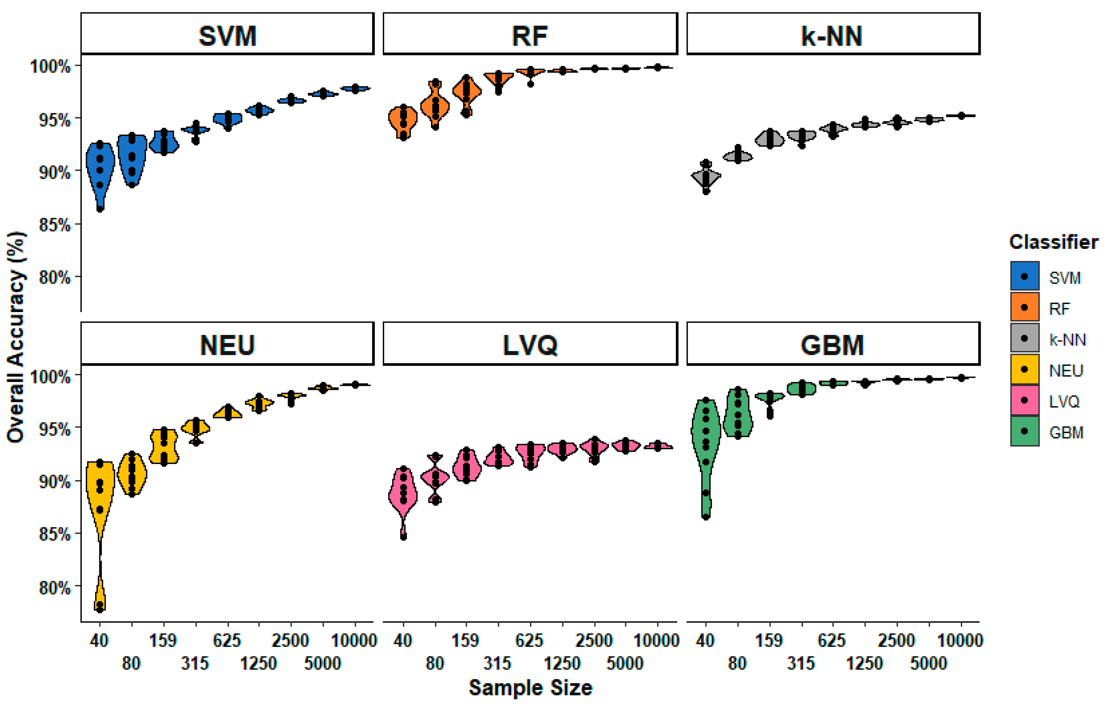
The mean values shown in Figure 3 hide considerable variation. This variation is therefore explored in Figure 4, which shows the distribution of individual classification accuracies for each classification method and sample size. It is notable for each classification method, variation in the overall accuracy decreases as the sample size increases. This is expected; a small sample is more likely to produce a wider range of potential outcomes. However, the figure also shows that there are considerable differences between classifiers. For example, both RF and k-NN appear to be good generalizers, in the sense that different training sets of the same size produce similar accuracies. In contrast, NEU and GBM produce a very wide range of accuracies with different training sets of the same size, especially for the smallest sample sets. When the number of training samples is very small, the specific samples chosen can be more important than the number of samples, even when the samples are drawn randomly, as in our experiments.
RF and GBM are notable for consistently achieving higher overall accuracy than the other four machine-learning algorithms, for all sample sizes. RF saw its highest average overall accuracy when trained from the 10,000-sample set (99.8%), and its lowest average accuracy when the training sample size was only 40 (94.7%). The lowest observed overall accuracy from an RF classification trained from 40 samples was 93.1%, while the highest was 99.8%, trained from 10,000 samples (Appendix A). The difference between the highest and lowest overall accuracies of the 90 RF classifications was 6.7%, the smallest range of any classifier.
Although the overall accuracy of the RF classifier increased as training sample size increased, RF overall accuracy began to plateau when the sample size reached 1250. The difference in accuracy between the worst performing RF classification using 1250 samples and highest performing RF classification trained from 10,000 samples was just 0.5%. This plateauing of the overall accuracy is perhaps not very surprising; when classifications reach very high overall accuracy, there is little potential for further increases in overall accuracy. However, it is worth noting that the user’s and producer’s accuracies of all classes, on average, continued to increase with sample size (data not shown). Using a single classification iteration as an example, the user’s accuracy of the water class increased from 66.0% when trained from 1250 samples to 80.2% when trained from 10,000 samples.
GBM provided comparable average overall accuracy to RF and was generally the second-most accurate classifier. When trained from sample sizes larger than 40, the difference in mean overall accuracy between GBM and RF was consistently less than 0.5% for all sample sizes, with RF slightly outperforming GBM, except when trained from 159 samples, where mean overall accuracy of GBM was 0.4% higher than RF. It is notable that individual iterations of GBM classifications occasionally provided higher levels of overall accuracy than RF. For example, when trained from 40 samples, the highest reported overall accuracy for GBM was 97.6%, while the highest overall accuracy for RF was 96.0% (Appendix A). When trained from samples sizes 80, 159, 315, and 625, some classification iterations of RF reported lower overall accuracies than the minimum reported accuracy by GBM for that sample size. Although GBM did have the second highest range of overall accuracy (Figure 4) when trained from a single sample set, at 11.1%, variability in overall accuracy rapidly decreased when sample size was greater than 159.
NEU is notable for being the classification method most dependent on training sample size. For a training sample size of 315 or larger, the NEU classifier was the third-most accurate classifier (Figure 3), with an average accuracy of 99.2% when trained with 10,000 samples. However, when trained with 40 samples, the average accuracy was 87.4%, the lowest average accuracy of the six methods. Of the six machine-learning algorithms investigated in this study, NEU had both the largest difference in average overall accuracy between the classifications trained from 10,000 and 40 samples, 11.7% (Figure 3), and the largest range of accuracy of classifications trained from the same sample size, at 14.0%, from a low of 77.7% to a high of 91.7% when trained from 40 samples (Figure 4). In addition, the 77.7% minimum accuracy for NEU was the lowest accuracy of all the 540 classifications.
The SVM classifier was generally intermediate in classification accuracy, generally ranking third or fourth in terms of average overall accuracy (Figure 3). Of all the classifiers, SVM showed the greatest increase in average overall accuracy, 0.6%, for the increase in sample size from 5000 to 10,000. This is notable, as it suggests that SVM benefits from very large sample sets (n = 10,000) and does not plateau in accuracy as much as RF and GBM classifiers do when the sample size becomes very large (e.g., 1000 and greater). This is likely due to larger samples containing more examples in the feature space that can be used as support vectors to optimize the hyperplane, and thus identify a more optimal class decision boundary for the SVM classification. SVM, when compared to the other five classifiers, showed generally intermediate to large ranges of individual overall accuracies for specific sample sizes (Figure 4). For example, SVM had the greatest range for 80 samples, and the second largest range when trained from 5000 and 10,000 samples.
k-NN produced the second-lowest average overall accuracy of the machine-learning classifiers for larger sample sizes, ranging from 315 to 10,000 (Figure 3). k-NN showed a tendency to plateau in accuracy when trained with large samples sets, with a difference in average overall accuracy of just 2.1% between training with 315 and 10,000 samples. Notably, k-NN also had the smallest range of overall accuracy when sample sizes ranged from 40 to 159 (Figure 4). This is surprising as k-NN and other lazy learning classifiers acquire their information entirely from the training set.
LVQ had the lowest average overall accuracy among all six classifiers, except when trained the smallest sample size of 40. The performance gap between LVQ and the other five classifiers generally increased with sample size. Average overall accuracy of LVQ plateaued when the sample size reached 315, with a less than 1.2% difference between the average accuracy of LVQ trained from 315 samples at 92.1%, and 10,000 samples at 93.2%. LVQ is notable for generally large variations in overall accuracy at specific sample sizes, at least in comparison to other classifiers, when trained from large sample sets, ranging from 2500 to 10,000 samples. This suggests that LVQ may be more sensitive to the composition of the dataset than similar methods such as k-NN, as random training samples are selected as codebook vectors to optimize the model.
Variability in overall classification accuracy, (i.e., Figure 4), such as that of SVM, has important implications that are illustrated in Figure 5. To create this figure, a single training set at each sample size (40, 80, etc.) was used to generate each of the six classifications. Although Figure 5 is broadly similar to Figure 3, the pattern is much noisy, with several cases where a larger number of training samples is actually less accurate than a smaller number. For example, for SVM, when the number of training samples increased from 40 to 80, the overall accuracy decreased by 3.9%, from 92.6% to 88.7%.
As indicated in Table 7 and Table 8, the lower performance of SVM trained with 80 samples compared to SVM trained with 40 samples was partly due the former classification’s lower user’s and producer’s accuracies for grassland and lower producer’s accuracy for forest, the majority class. It is surprising that these two classes, the largest classes by area, should vary so in accuracy. However, since the training samples are selected randomly, and SVM focuses exclusively on support vectors (i.e., potentially confused samples) for separating classes, it suggests SVM may be inherently more inconsistent in its likely accuracy for a particular size. For the SVM trained with just 40 samples, the water class, which has only 4 training samples, resulted in the second-lowest producer’s accuracy for all 54 classifications in this series, at 47.8%. This is evident in Figure 6 in the visual analysis section.
The training samples at each size were selected independently, which means that the training sample with 80 samples is unlikely to include many, if any, of the samples from the 40-sample set. In a real-world application, an analyst considering expanding a training data set would naturally want to include any previously collected data in the expanded data set. Thus, an analyst deciding to add to training data set would not necessarily experience the kind of decline in accuracies shown in Figure 5. However, the graph does illustrate that the benefits of increasing the sample size are not always predictable, and why it can be so difficult to generalize from individual experiments, particularly for classification methods such as SVM that appear to be quite sensitive to the specific training samples chosen.

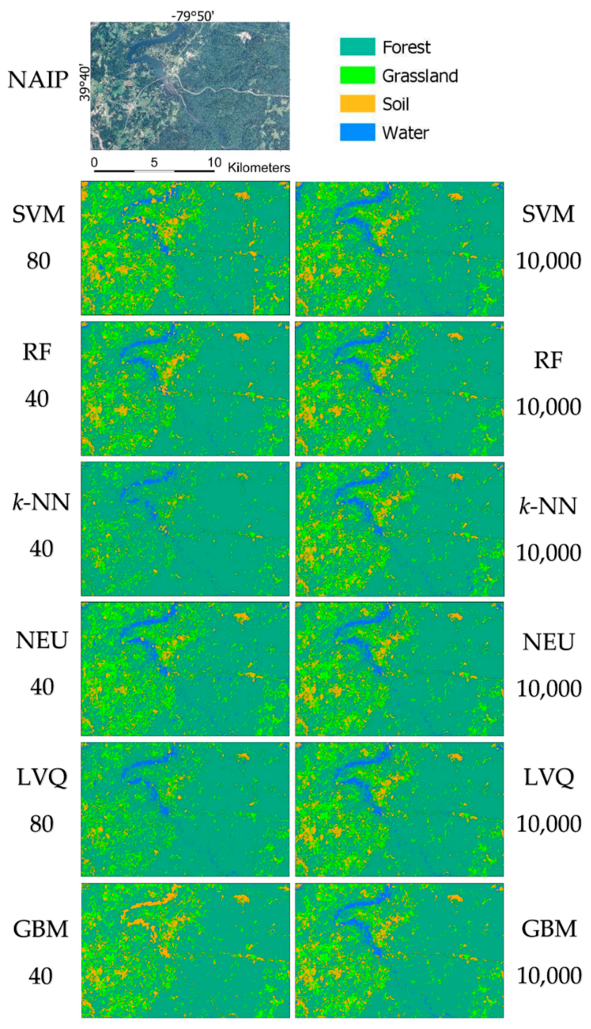
3.2. Visual Analysis

Figure 6 illustrates example classifications for a subset region (see Figure 1 for the subset location). For consistency, for each sample size (e.g., 40 samples), the same training data set was used for each classifier, and the overall accuracy of the resulting classifications is graphed in Figure 5. Only the classifications with the highest and lowest overall accuracy for each classifier are shown in Figure 6. In this iteration of the classifications, the SVM and LVQ classifications trained from 80 samples produced a lower overall accuracy than classifications trained from 40 samples.
Visual inspection of the example classifications (Figure 6) indicates clear improvements in classifications trained from larger sample sets. Most of the errors were misclassifications of the soil and water classes. Notably, in the SVM classification trained from 80 samples, and the GBM classification trained from 40 samples many water objects were misclassified as soil and vice versa. These errors were reduced in the SVM classification trained from 10,000 samples. Although the user’s accuracy of water only increased by 2.5% between the SVM classification trained from 80 samples and the SVM classification trained from 10,000 samples, the producer’s accuracy of the water class improved by 39.1% and the user’s accuracy of the soil class improved by 35.1% (Table 9).
Visual inspection of the best overall classification from the sample classifications, RF trained from 10,000 samples, displayed in Figure 6, shows that while there were still some clear misclassifications of the water class, especially in the large lake located near 39°40′, −79°50′, and noted by the red circle in Figure 7, overall classification quality was high.
In this iteration all classifiers generally mapped the forest class well, with the lowest user’s accuracy reported as 90.5% with k-NN, and the lowest producer’s accuracy reported as 89.0% with NEU, in both instances trained from 40 samples. As forest was the majority class in this case, comprising nearly 81% of the validation set, the good performance of the forest class by all classifiers contributed to relatively high overall accuracies for all classifications.

3.3. Computational Complexity

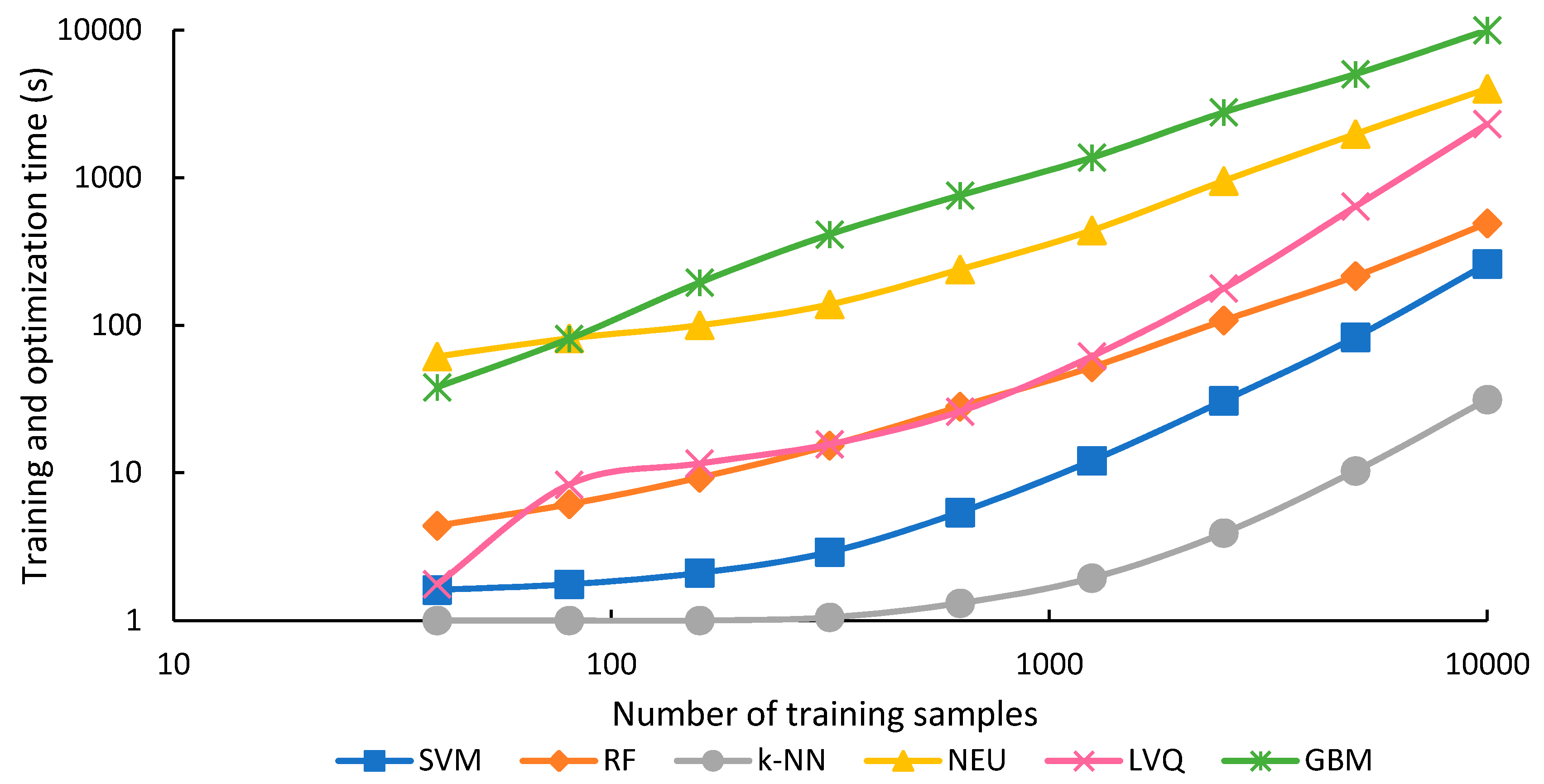
The training and optimization time for each classifier for each sample size is shown in 
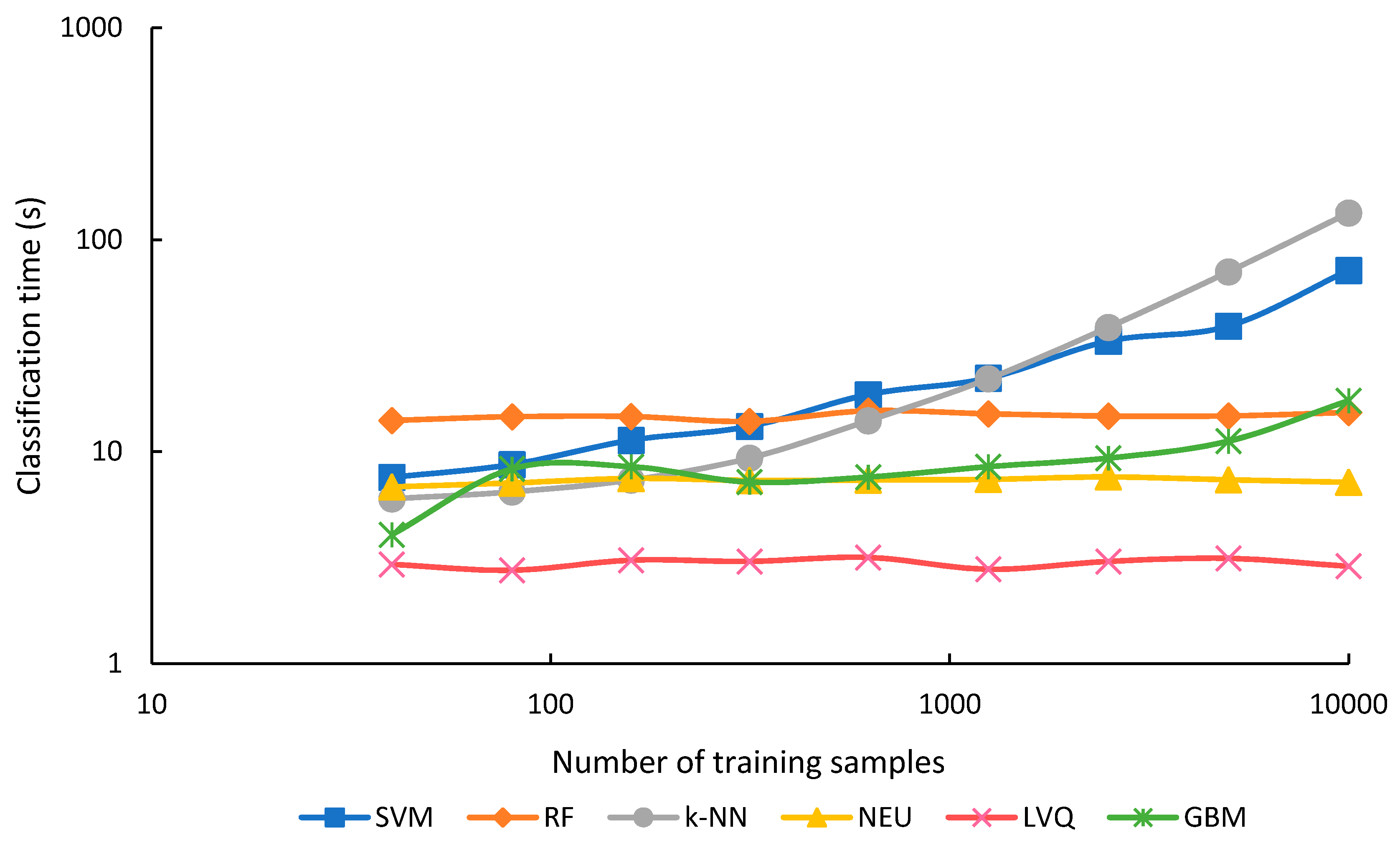
Figure 8, and the classification time in Figure 9. Training and optimization time generally took much longer than classification for all classifiers, except for k-NN and SVM when training set sizes were smaller than 2500, and RF when training set size was 159 or smaller. Training and optimization time generally increased for all classifiers as the training set size increased (Figure 8). This is expected for most classifiers. However, for k-NN, a lazy classifier, the increased time is presumably associated with the optimization, since this method has no training. In contrast to training and optimization time, classification time was generally unaffected by training sample size, except for SVM and k-NN, and to a smaller degree, GBM (Figure 9). Summing both training and classification time indicates that GBM was generally the most expensive algorithm in terms of processing time. NEU was second, LVQ third, RF fourth, SVM fifth, and k-NN was the fastest of all algorithms.
GBM was generally the slowest algorithm in terms of training and optimization time (Figure 8), and for all but the sample sets with 40 and 80 samples, was 2 to 3 times slower than the second-slowest algorithm, NEU. GBM was also very expensive in terms of computational resources; training the GBM classifier with 10,000 samples consumed over 27 GB of memory. GBM was generally intermediate in terms of classification time (Figure 9). GBM was sensitive to numbers of training samples for the very smallest and largest training sets, but classification time was relatively constant for training sets between 80 and 2500 samples.
NEU was also slow in training and optimization time, almost two orders of magnitude slower than RF, k-NN, and SVM. However, NEU was generally intermediate to fast in terms classification time. Overall, long processing times of NEU classifiers compared to other supervised machine-learning algorithms was also noted in [2].
LVQ training and optimization time was the most sensitive to sample size, increasing 1310-fold, as the sample size increased from 40 to 10,000 samples. However, even with 10,000 samples, LVQ was less slow than GBM and NEU. On the other hand, LVQ was notably faster in classification time than all the other classifiers, irrespective of sample size.
RF generally took 4 times as long as SVM to train and optimize, though this difference declined for larger numbers of training samples, for example, to only 1.8 times as long with 10,000 samples. This suggests that the training and optimizing time for SVM does not scale as efficiently as RF with increasing sample size. Furthermore, RF training time could potentially be reduced by reducing the value of the parameter that determines the number of trees. Because RF classification was not affected by sample size, but SVM was, the rank of the two classifiers in terms of classification speed switched at a sample size of 315. Below this number of samples, SVM was faster, above it, RF was faster.
The k-NN classifier was by far the most efficient classifier in terms of training and optimizing time, with the time for 40, 80, and 159 sample sizes taking less than 1 s, and the time for 2500 samples taking nearly 4 s. However, as a lazy learning classifier, requiring each unknown to be compared to the original training data, k-NN classification was the method most sensitive to the training sample size. For training samples of 2500 and greater, it required the longest time for classification. In addition, the computation memory demands of k-NN are potentially substantial for large numbers of training samples. For example, one approach to optimize the k-NN search is to store in memory the distance between every pair of training instances, which tends to scale as a function of n2, where n is the number of training samples [81].

4. Discussion

Based on the performance of the supervised machine-learning classifications, our results show that machine-learning classifiers vary in accuracy and in required computation resources in response to training set size. Similar to observations made by [10,11], we found that classifier performance generally improved with larger sample sizes. However, we also observed that for some classifiers, particularly RF, GBM, LVQ and k-NN, increasing sample set size after a certain point did not substantially improve classification accuracy, even when using a training set 2 orders of magnitude larger in size, while computational demands increase. In comparison, SVM and NEU continued to benefit from larger sample sizes through increases in overall accuracy, as well as class user’s and producer’s accuracies.
In detail, the effects of sample size vary with the different classifiers. In the case of the RF and GBM algorithms, increasing the sample size continued to improve the user’s and producer’s accuracies of minority classes, even when the overall accuracy did not notably increase. With the SVM and NEU algorithms, we observed that overall accuracy continued to rise when trained from larger sample sets. However, both GBM and NEU algorithms were consistently the most expensive in terms of training and optimization time but were relatively quick in terms of classification time when trained with moderate or large training data sets. Although GBM provided similar levels of overall accuracy to RF, the computational demands of the GBM classifier were far greater than RF. For example, with trainings sets of 625 or more samples, GBM required more than 15 times the total processing time of RF. GBM’s longer training time is not unexpected, as trees in GBM are built sequentially, contrasting with RF’s trees which are trained independently and can be built in parallel. In addition, the parameterization of GBM was more complex than RF, as three parameters were tuned with GBM, compared to a single parameter with RF. In general, we observed that training time for classifiers with more tuning parameters (GBM, NEU, LVQ) was longer than classifiers with less parameters (k-NN, SVM, RF). However, it should be noted that computational time of all classifiers may vary depending on the programming language and environment they are executed in, and there may be more computationally efficient platforms or implementations than the code used in this analysis. With advances in cloud and high-performance computing environments incorporating parallel processing, the specific implementation or platform of choice may be less of a concern. In addition, while GBM was more computationally intensive than RF within the range of sample sizes examined in this analysis, RF may experience memory and search issues when using incredibly large training datasets. Although our sample size range was selected for the purpose of investigating differences between classification methods, future research should be conducted on classifier responses to extremely large training sets.
Although larger sample sets generally led to an improvement in overall accuracy of the k-NN algorithm, overall accuracy of the k-NN classifier did not improve as much as NEU and SVM when trained from larger sample sets. However, the k-NN classifier was much faster than all other classifiers, especially with larger training sets. Although LVQ outperformed NEU with small sample sizes, overall accuracies of LVQ classifications plateaued quickly with relatively small sample sizes, and generally underperformed compared to the other five algorithms, especially with large training sets, which suggests that additional training samples may not be beneficial for improving accuracy beyond a certain threshold. Notably, when trained with sets of intermediate to large size (for example, 625 samples and large), the replications of the LVQ classifications produced a large range accuracy values compared to the other classifiers. This suggests that LVQ is more sensitive to the composition of the training set, even with large training sets, compared to the other five classification methods. Also, training time for LVQ did not scale well to larger sample sets.
However, variability in overall accuracy when trained from different training sets tended to decrease with larger sample sets for all classification methods. This trend was observed for all six classifiers investigated in this study. This suggests that individual samples in smaller sample sets may have more of an effect on classification performance, which could lead to variations in overall accuracy. Thus, training on larger samples sets is recommended for robust measures of overall accuracy. In our previous work [34], we showed that training samples selected randomly tend to outperform those selected deliberatively. With a deliberative sample, the variability in the representative nature of individual samples may be even greater than was observed in our study (as shown in Figure 4), which would further reinforce the point that larger sample sizes tend to favor greater accuracy. Furthermore, extremely small sample sets, where there are as few as four training samples available for a particular class can be problematic for certain classification methods, such as SVM, NEU, LVQ, and GBM and may result in poor performance in terms of overall accuracy, as the classifier may fail to predict that an observation will come from a minority class with so few samples.
Although we reported specific accuracy metrics for the classifications conducted in these experiments, the performance of classifiers may vary depending on several factors, such as the number of classes, the quality of training data, and the size and composition of the study area. Nevertheless, several general insights and recommendations can be made from this study:
  • Although in general, analysts should collect as many training samples as possible, some classifiers, such as RF, GBM, k-NN, and LVQ, may not benefit from increased sample size beyond a certain threshold where the classifier has appeared to have reached its maximum its accuracy, thus additional sample collection may not be useful. If training samples have already been collected, and the analyst would like to know whether additional samples might result in a higher accuracy, one possibility would be to test whether a plateau has already been reached in the accuracy, for example, by plotting accuracy as a function of sample size for the data already collected.
  • Classifications trained from larger sample sizes tended to show less variability in overall accuracy when trained from different sample sets than classifications trained from smaller sample sets. Larger training sets are recommended over smaller training sets for robustness in overall accuracy. This observation has important implications for research design for experiments that investigate classifier performance. Replication, with different selections of training data, is crucial for experiments that use training data with small numbers of samples, as in such circumstances the relative performance of classifiers can depend more on the particular training samples selected than the number of samples.
  • Computational time should be considered by the analyst, especially if larger training sample sizes are used, as some machine-learning algorithms are more expensive than others in terms of computation time for training and classification processes, especially with larger training sets.
  • As the performance of a supervised classification trained from a fixed training set size may be hard to predict in advance, multiple machine-learning classification algorithms should be investigated for remote sensing analyses.
This study had several limitations. This was a single investigation of the effects of training set size on supervised machine-learning classifiers. Our study area, though covering a large geographic area, is broadly homogenous and dominated by a single class. Although a simpler analysis, for example, a binary classification such as forest/non-forest may have been more straightforward to interpret, by including four classes, and by including the rare class of water, the study is perhaps more representative of typical remote sensing studies. In addition, this work used a GEOBIA, rather than a pixel-based, approach to classification. Although other investigations involving classifiers and sample size such as [11] suggest that GEOBIA approaches provide overall accuracies that are superior to pixel-based approaches, we focused on investigating general trends of classifier response to increasing training set size in terms of accuracy and computational complexity, rather than examining differences in performance between pixel- and object-based classification approaches. Although pixel-based data may not contain the geometric predictor variables provided by GEOBIA data, we do not believe that the choice of classification approach would have a large effect on the general trends in observations reported here, even though specific values of accuracy and computational measures would likely change between the two approaches.
Future research should examine the effects of other aspects of classification in conjunction with sample sizes, for example feature elimination and ranking processes, and the inclusion of additional, non-beneficial predictor variables that may increase computational complexity and possibly classification error. In addition, an investigation on training set size and classifier response that incorporates multiple datasets, study areas, and sensor types would be valuable.

5. Conclusions

This analysis explored the effects of the number of training samples, varying from 40 to 10,000, on six supervised machine-learning algorithms, SVM, RF, k-NN, NEU, LVQ, GBM, to classify a large-area HR remotely sensed dataset. Although it is well known from previous studies that larger training sets typically provide superior classification performance over smaller training sets [1], our study found considerable variation in how six machine-learning classifiers responded to changes in training sample size. Furthermore, our study extends previous comparisons of machine-learning classifier dependence on sample size, [10,11,82] by incorporating RF, SVM, NEU, GBM, and k-NN, which tend to be among the most commonly used classifiers [2] as well as LVQ, a method widely used in non-remote sensing disciplines. We also evaluated performance over a large range compared to previous studies.
Overall, machine-learning methods varied considerably in their response to changes in sample size. Even with the same classifier, and the same number of training samples, accuracy varied between replicates that used different training samples. Therefore, we recommend that a good practice for any project involving supervised classifications of remotely sensed data would be to investigate multiple machine-learning classification methods, as some machine-learning classifiers may provide better accuracy than others depending on the size of the training set.
If it is not feasible to test multiple methods, RF appears to be the best all-round choice as a classifier, at least over the range of training sample sizes studied in this experiment, given RF’s superior performance over the other machine-learning algorithms. Although GBM provided similar measures of overall accuracy to RF, GBM was far more computationally expensive in terms of processing time and resources and generally did not provide an advantage in overall accuracy. RF and GBM were found to be more accurate than the other classifiers, irrespective of training sample size, so much so that they tended to outperform the other supervised classification approaches, even when the other classifiers were given much larger training sets. For example, RF and GBM using 315 samples provided a higher overall accuracy than the other four classification methods, even when given more than 30 times the number of training samples. Ref. [82] also found that RF outperformed other classifiers such as SVM and k-NN. In summary, RF was found to be a particularly good choice, especially if there are only limited training data. We also note that methods such as Xgboost [77] expand on GBM by adding regularization parameters to penalize the complexity of the classification trees. Methods such as this can also see drastic computational speed increases under the right conditions such as sparse data and access to high-performance computing environments.
Although SVM and NEU resulted in relatively low accuracy with smaller sample sets, the accuracy continued to improve with larger sample sizes, which suggests that if available, larger sample sizes are recommended. However, if using large sample sets, training times for NEU may become prohibitive. On the other hand, once trained, NEU is one of the faster classification algorithms when trained with large training data sets. SVM training time seemed to scale to larger sample sets more efficiently than NEU. LVQ and k-NN typically provided lower overall accuracy than RF, GBM, SVM, and NEU, especially as training set size increased. Although overall accuracy of k-NN increased with larger training sample sizes, the increase in accuracy was smaller than that of SVM, GBM, and NEU classifiers. However, k-NN had the shortest total computational time (optimization, training and classification) of all classifiers, regardless of sample size. LVQ was generally the worst performing classifier and displayed relatively large variations in overall accuracy when trained from different training sets of identical size, even with large training sets. In addition, LVQ did not scale well in terms of training time when given large sample sets. LVQ is thus not recommended, unless training sample is small, in which case it can potentially provide rapid processing and at least average classification accuracy.

Author Contributions

Conceptualization, C.A.R.; methodology, C.A.R., T.A.W., A.E.M. and B.S.P.; software, C.A.R., A.E.M.; validation, C.A.R.; formal analysis, C.A.R.; investigation, C.A.R.; resources, C.A.R.; data curation, C.A.R.; writing—original draft preparation, C.A.R.; writing—review and editing, C.A.R., T.A.W., A.E.M. and B.S.P.; visualization, C.A.R.; supervision, C.A.R.; project administration, C.A.R. and T.A.W.; funding acquisition, C.A.R. All authors have read and agreed to the published version of the manuscript.

Funding

The APC was funded by West Virginia University Open Access Author Fund (OAAF), and the Department of Management Information Systems, John Chambers College of Business and Economics at West Virginia University.

Institutional Review Board Statement

Not applicable.

Informed Consent Statement

Not applicable.

Data Availability Statement

Data sharing not applicable.

Acknowledgments

The authors would like to thank the anonymous referees whose comments greatly strengthened this paper.

Conflicts of Interest

The authors declare no conflict of interest.

Appendix A. Overall Accuracies by Classification Method, Iteration, and Sample Size

Table A1. Overall Accuracies of Radial Basis Function Support Vector Machines (SVM) Classifications.
Radial Basis Function Support Vector Machines (SVM)
Sample Size
408015931562512502500500010,000
Classification Iteration191.1%93.3%91.8%93.9%95.3%95.8%96.6%97.2%97.7%
291.2%89.8%92.8%94.0%95.3%95.3%96.8%97.2%97.9%
390.1%92.9%93.8%93.9%94.9%96.1%97.1%97.5%97.8%
492.4%91.5%92.4%93.7%94.8%95.4%96.4%97.3%98.0%
588.7%91.2%92.4%93.7%94.7%95.6%96.5%97.2%97.6%
686.3%90.1%93.5%94.0%95.4%96.0%96.5%97.0%97.9%
790.1%92.9%92.3%92.8%94.0%95.7%96.8%97.0%97.8%
888.6%91.3%91.9%93.0%94.7%95.6%96.6%97.4%97.8%
991.2%92.9%93.6%94.5%95.2%95.9%96.7%97.3%97.8%
1092.6%88.7%92.8%93.9%94.6%95.7%96.6%97.1%97.6%
Table A2. Overall Accuracies of Random Forests (RF) Classifications.
Random Forests (RF)
Sample Size
408015931562512502500500010,000
Classification Iteration195.5%98.2%98.2%98.5%98.1%99.4%99.7%99.7%99.8%
294.5%98.4%97.9%98.0%99.3%99.5%99.8%99.8%99.7%
396.0%95.6%97.5%99.3%99.6%99.6%99.7%99.6%99.8%
494.4%96.7%97.6%97.4%99.5%99.4%99.6%99.7%99.8%
595.1%95.2%95.7%98.6%99.4%99.3%99.6%99.7%99.8%
693.4%96.6%97.3%99.2%99.5%99.5%99.7%99.7%99.8%
793.1%95.7%95.2%99.2%99.1%99.5%99.6%99.7%99.8%
894.4%94.1%97.4%99.3%99.5%99.4%99.6%99.7%99.8%
995.2%96.2%98.8%98.9%99.5%99.5%99.6%99.8%99.8%
1095.5%96.1%96.8%99.0%99.2%99.4%99.7%99.7%99.8%
Table A3. Overall Accuracies of k-Nearest Neighbors (k-NN) Classifications.
k-Nearest Neighbors (k-NN)
Sample Size
408015931562512502500500010,000
Classification Iteration189.2%91.5%93.1%93.6%94.4%94.5%94.6%94.8%95.3%
288.8%91.1%92.5%92.3%93.3%94.4%94.5%94.9%95.2%
389.1%91.6%93.5%93.7%94.0%94.8%94.5%95.1%95.2%
489.7%91.4%92.9%93.5%93.9%94.2%94.5%94.8%95.2%
589.7%91.1%92.9%93.5%93.6%94.4%94.7%94.9%95.2%
688.0%91.0%92.8%93.8%94.2%94.3%94.8%94.8%95.1%
790.9%91.2%92.3%93.0%94.0%94.1%94.5%95.0%95.2%
890.5%92.2%93.3%93.1%93.2%94.1%94.3%94.8%95.2%
989.6%91.7%92.5%93.1%94.0%94.5%94.1%95.0%95.2%
1089.5%91.2%93.7%93.3%94.2%94.3%95.0%94.7%95.2%
Table A4. Overall Accuracies of Single-Layer Perceptron Neural Networks (NEU) Classifications.
Single-Layer Perceptron Neural Networks (NEU)
Sample Size
408015931562512502500500010,000
Classification Iteration191.7%92.5%91.9%95.3%95.9%96.5%98.2%98.7%99.1%
291.5%91.1%92.1%95.7%96.5%97.4%98.1%98.7%99.1%
389.7%92.0%94.0%95.5%96.4%97.4%98.1%98.8%99.2%
489.8%89.2%92.4%93.5%96.6%96.7%97.7%98.7%99.0%
578.2%90.9%94.1%94.8%96.2%97.5%98.0%98.8%99.1%
687.3%91.4%94.5%95.1%96.2%96.8%98.0%98.7%99.1%
789.1%89.9%91.6%93.5%96.1%97.4%97.2%98.5%99.0%
877.7%90.2%92.3%94.7%97.0%97.3%97.8%98.9%99.0%
991.6%90.3%94.8%95.0%95.9%97.3%98.1%98.7%99.0%
1087.2%88.7%93.5%94.7%96.0%98.0%98.1%99.0%99.0%
Table A5. Overall Accuracies of Learning Vector Quantization (LVQ) Classifications.
Learning Vector Quantization (LVQ)
Sample Size
408015931562512502500500010,000
Classification Iteration190.2%92.3%90.0%92.8%93.4%92.7%93.9%93.5%93.5%
289.3%90.3%91.3%91.8%91.5%92.7%93.4%92.7%93.2%
388.2%90.6%92.9%93.1%93.4%93.2%92.8%93.8%93.6%
488.0%89.8%90.0%92.3%92.9%93.3%93.1%92.9%93.1%
588.2%88.2%91.2%91.8%91.9%92.7%93.3%93.4%93.0%
684.6%90.3%92.4%91.3%92.7%93.3%92.1%93.2%93.1%
788.1%87.9%92.1%91.6%92.5%92.1%92.7%93.6%93.5%
890.3%92.3%91.4%91.6%91.3%92.9%91.7%92.9%93.0%
988.8%90.5%90.9%92.2%93.3%93.5%93.3%93.4%93.2%
1091.1%89.8%90.7%92.3%93.0%93.0%93.3%93.1%93.3%
Table A6. Overall Accuracies of Gradient Boosted Trees (GBM) Classifications.
Gradient Boosted Trees (GBM)
Sample Size
408015931562512502500500010,000
Classification Iteration196.5%97.3%97.9%98.1%99.0%99.1%99.6%99.6%99.8%
294.7%98.1%97.5%98.2%99.2%99.1%99.6%99.6%99.7%
394.7%97.2%97.8%99.3%99.3%99.2%99.6%99.6%99.7%
495.8%96.2%98.1%98.6%99.4%99.4%99.6%99.7%99.8%
591.8%95.4%96.0%98.9%99.1%99.4%99.5%99.6%99.7%
686.6%95.2%97.9%99.1%99.4%99.4%99.5%99.6%99.8%
788.8%94.2%96.6%98.5%99.1%99.4%99.4%99.6%99.7%
893.2%94.4%98.3%98.9%99.4%99.4%99.5%99.6%99.7%
997.6%98.6%97.9%98.7%99.0%99.4%99.5%99.6%99.8%
1093.6%95.4%98.1%98.3%99.4%99.4%99.5%99.7%99.7%

References

  1. Foody, G.M.; Mathur, A.; Sanchez-Hernandez, C.; Boyd, D.S. Training set size requirements for the classification of a specific class. Remote Sens. Environ. 2006, 1, 1–14. [Google Scholar] [CrossRef]
  2. Maxwell, A.E.; Warner, T.A.; Fang, F. Implementation of machine-learning classification in remote sensing: An applied review. Int. J. Remote Sens. 2018, 39, 2784–2817. [Google Scholar] [CrossRef] [Green Version]
  3. Raczko, E.; Zagajewski, B. Comparison of support vector machine, random forest and neural network classifiers for tree species classification on airborne hyperspectral APEX images. Eur. J. Remote Sens. 2017, 50, 144–154. [Google Scholar] [CrossRef] [Green Version]
  4. Samaniego, L.; Schulz, K. Supervised Classification of Agricultural Land Cover Using a Modified k¬-NN Technique (MNN) and Landsat Remote Sensing Imagery. Remote Sens. 2009, 1, 875–895. [Google Scholar] [CrossRef] [Green Version]
  5. Foody, G.M.; McCulloch, M.B.; Yates, W.B. The effect of training set size and composition on artificial neural network classification. Int. J. Remote Sens. 1995, 16, 1707–1723. [Google Scholar] [CrossRef]
  6. Millard, K.; Richardson, M. On the Importance of Training Data Sample Selection in Random Forest Image Classification: A Case Study in Peatland Ecosystem Mapping. Remote Sens. 2015, 7, 8489–8515. [Google Scholar] [CrossRef] [Green Version]
  7. Heydari, S.S.; Mountrakis, G. Effect of classifier selection, reference sample size, reference class distribution and scene heterogeneity in per-pixel classification accuracy using 26 Landsat sites. Remote Sens. Environ. 2017, 204. [Google Scholar] [CrossRef]
  8. Noi, P.T.; Kappas, M. Comparison of Random Forest, k-Nearest Neighbor, and Support Vector Machine Classifiers for Land Cover Classification Using Sentinel-2 Imagery. Sensors 2018, 18, 18. [Google Scholar] [CrossRef] [Green Version]
  9. Myburgh, G.; Van Niekerk, A. Effect of feature dimensionality on object-based land cover classification: A comparison of three classifiers. S. Afr. J. Geomat. 2013, 2, 13–27. [Google Scholar]
  10. Qian, Y.; Zhou, W.; Yan, J.; Li, W.; Han, L. Comparing Machine Learning Classifiers for Object-Based Land Cover Classification Using Very High Resolution Imagery. Remote Sens. 2015, 7, 153–168. [Google Scholar] [CrossRef]
  11. Shang, M.; Wang, S.; Zhou, Y.; Du, C. Effects of Training Samples and Classifiers on Classification of Landsat-8 Imagery. J. Indian Soc. Remote Sens. 2018, 46, 1333–1340. [Google Scholar] [CrossRef]
  12. Belgiu, M.; Drăgut, L. Random forest in remote sensing: A review of applications and future directions. ISPRS J. Photogram. Remote Sens. 2016, 114, 24–31. [Google Scholar] [CrossRef]
  13. Lawrence, R.L.; Moran, C.J. The AmericaView Classification Methods Accuracy Project: A Rigorous Approach for Model Selection. Remote Sens. Environ. 2015, 170, 115–120. [Google Scholar] [CrossRef]
  14. Neves, J.C.; Vieira, A. Improving bankruptcy prediction with Hidden Layer Learning Vector Quantization. Euro. Account. Rev. 2011, 15, 253–271. [Google Scholar] [CrossRef]
  15. Ahn, K.K.; Nguyen, H.T.C. Intelligent Switching control of pneumatic muscle robot arm using learning vector quantization network. Mechatronics 2007, 17, 225–262. [Google Scholar] [CrossRef]
  16. Yang, M.; Lin, K.; Liu, H.; Lirng, J. Magnetic resonance imaging segmentation techniques using batch-type learning vector quantization. Magn. Reson. Imaging 2007, 25, 265–277. [Google Scholar] [CrossRef]
  17. Ma, L.; Li, M.; Ma, X.; Cheng, K.; Du, P.; Liu, Y. A review of supervised object-based land-cover image classification. ISPRS J. Photogram. Remote Sens. 2017, 130, 277–293. [Google Scholar] [CrossRef]
  18. Blaschke, T. Object based image analysis for remote sensing. ISPRS J. Photogram. Remote Sens. 2010, 65, 2–16. [Google Scholar] [CrossRef] [Green Version]
  19. Maxwell, A.E.; Warner, T.A.; Vanderbilt, B.C.; Ramezan, C.A. Land cover classification and feature extraction from National Agriculture Imagery Program (NAIP) Orthoimagery: A review. Photogram. Eng. Remote Sens. 2017, 83, 737–747. [Google Scholar] [CrossRef]
  20. WVU NRAC. Aerial Lidar Acquistion Report: Preston County and North Branch (Potomac) LIDAR *.LAS 1.2 Data Comprehensive and Bare Earth. West Virginia Department of Environmental Protection. Available online: http://wvgis.wvu.edu/lidar/data/WVDEP_2011_Deliverable4/WVDEP_deliverable_4_Project_Report.pdf (accessed on 1 December 2018).
  21. Yan, W.Y.; Shaker, A.; El-Ashmawy, N. Urban land cover classification using airborne LiDAR data: A review. Remote Sens. Environ. 2015, 158, 295–310. [Google Scholar] [CrossRef]
  22. ESRI. ArcGIS Desktop: Release 10.5.1; Environmental Systems Research Institute: Redlands, CA, USA, 2017. [Google Scholar]
  23. Maxwell, A.E.; Warner, T.A.; Strager, M.P.; Conley, J.F.; Sharp, A.L. Assessing machine-learning algorithms and image- and lidar-derived variables for GEOBIA classification of mining and mine reclamation. Int. J. Remote Sens. 2015, 36, 954–978. [Google Scholar] [CrossRef]
  24. Petrie, G.; Toth, C.K. Airborne and Spaceborne Laser Profilers and Scanners. In Topographic Laser Ranging and Scanning: Principles and Processing; Shan, J., Toth, C.K., Eds.; CRC Press: Boca Raton, FL, USA, 2008. [Google Scholar]
  25. Lear, R.F. NAIP Quality Samples. United States Department of Agriculture Aerial Photography Field Office. Available online: https://www.fsa.usda.gov/Internet/FSA_File/naip_quality_samples_pdf.pdf (accessed on 28 December 2018).
  26. Baatz, M.; Schäpe, A. Multiresolution Segmentation—An Optimization Approach for High Quality Multi-Scale Image Segmentation; Angewandte Geographische Informations-Verarbeitung XII; Strobl, T., Blaschke, G.G., Eds.; Wichmann Verlag: Karlsruhe, Germany, 2000; pp. 12–23. [Google Scholar]
  27. Drăgut, L.; Csillik, O.; Eisank, C.; Tiede, D. Automated parameterization for multi-scale image segmentation on multiple layers. ISPRS J. Photogram. Remote Sens. 2014, 88, 119–127. [Google Scholar] [CrossRef] [Green Version]
  28. Kim, M.; Warner, T.A.; Madden, M.; Atkinson, D. Multi-scale texture segmentation and classification of salt marsh using digital aerial imagery with very high spatial resolution. Int. J. Remote Sens. 2011, 32, 2825–2850. [Google Scholar] [CrossRef]
  29. Arvor, D.; Durieux, L.; Andrés, S.; Laporte, M. Advances in Geographic Object-Based Image Analysis with Ontologies: A review of main contributions and limitations from a remote sensing perspective. ISPRS J. Photogram. Remote Sens. 2013, 82, 125–137. [Google Scholar] [CrossRef]
  30. Hay, G.J.; Castilla, G.; Wulder, M.A.; Ruiz, J.R. An automated object-based approach for the multiscale image segmentation of forest scenes. Int. J. Appl. Earth Obs. Geoinf. 2005, 7, 339–359. [Google Scholar] [CrossRef]
  31. Kim, M.; Madden, M.; Warner, T.A. Forest type mapping using object-specific texture measures from multispectral IKONOS imagery: Segmentation quality and image classification issues. Photogram. Eng. Remote Sens. 2009, 75, 819–829. [Google Scholar] [CrossRef] [Green Version]
  32. Drăguţ, L.; Tiede, D.; Levick, S.R. ESP: A tool to estimate scale parameter for multiresolution image segmentation of remotely sensed data. Int. J. Geo-Inf. 2010, 24, 859–871. [Google Scholar] [CrossRef]
  33. Salehi, B.; Zhang, Y.; Zhong, M.; Dey, V. Object-Based Classification of Urban Areas Using VHR Imagery and Height Points Ancillary Data. Remote Sens. 2012, 4, 2256–2276. [Google Scholar] [CrossRef] [Green Version]
  34. Ramezan, C.A.; Warner, T.A.; Maxwell, A.E. Evaluation of Sampling and Cross-Validation Tuning Strategies for Regional-Scale Machine Learning Classification. Remote Sens. 2019, 11, 185. [Google Scholar] [CrossRef] [Green Version]
  35. Stehman, S.V.; Foody, G.M. Accuracy assessment. In The SAGE Handbook of Remote Sensing; Warner, T.A., Nellis, M.D., Foody, G.M., Eds.; Sage Publications Ltd.: London, UK, 2009; pp. 129–145. ISBN 9781412936163. [Google Scholar]
  36. Kuhn, M. Caret: Classification and Regression Training. R Package Version 6.0-71. 2016. Available online: https://CRAN.R-project.org/package=caret (accessed on 18 February 2019).
  37. Meyer, D. Support Vector Machines: The Interface to Libsvm in Package e1071. R package Version 6.0-71. 2012. Available online: https://CRAN.R-project.org/package=e1071 (accessed on 18 February 2019).
  38. Wright, M.N.; Ziegler, A. Ranger: A fast implementation of random forests for high dimensional data in C++ and R. J. Stat. Softw. 2017, 77, 1–17. [Google Scholar] [CrossRef] [Green Version]
  39. Ripley, B.; Venables, W. Feed-Forward Neural Networks and Multinomial Log-Linear Models. R Package Version 7.3-12. 2016. Available online: https://cran.r-project.org/web/packages/nnet/index.html (accessed on 10 October 2020).
  40. Ripley, B.; Venables, W. Functions for Classification, including k-nearest neighbour, Learning Vector Quantization, and Self-Organizing Maps. R. Package Version 7.3-12. 2015. Available online: https://cran.r-project.org/web/packages/class/index.html (accessed on 10 October 2020).
  41. Greenwell, B.; Boehmke, B.; Cunningham, J. Generalized Boosted Regression Models. R Package Version 2.1.8. 2020. Available online: https://cran.r-project.org/web/packages/gbm/index.html (accessed on 10 October 2020).
  42. Cortes, C.; Vapnik, V. Support-Vector Networks. Mach. Learn. 1995, 20, 273–297. [Google Scholar] [CrossRef]
  43. Pal, M. Kernel Methods in Remote Sensing: A Review. ISH J. Hydraul. Eng. 2012, 15, 194–215. [Google Scholar] [CrossRef]
  44. Mountrakis, G.; Im, J.; Ogole, C. Support Vector machines in remote sensing: A review. ISPRS J. Photogram. Remote Sens. 2010, 66, 247–259. [Google Scholar] [CrossRef]
  45. Khatami, R.; Mountrakis, G.; Stehman, S.V. A meta-analysis of remote sensing research on supervised pixel-based land-cover image classification processes: General guidelines for practitioners and future research. Remote Sens. Environ. 2016, 177, 89–100. [Google Scholar] [CrossRef] [Green Version]
  46. Sharma, V.; Baruah, D.; Chutia, D.; Raju, P.; Bhattacharya, D.K. An assessment of support vector machine kernel parameters using remotely sensed satellite data. In Proceedings of the IEEE International Conference on Recent Trends in Electronics, Information & Communication Technology (RTEICT), Bangalore, India, 20–21 May 2016. [Google Scholar] [CrossRef]
  47. Zhu, G.; Blumberg, D.G. Classification using ASTER data and SVM algorithms; the case study of Beer Sheva, Israel. Remote Sens. Environ. 2002, 80, 233–240. [Google Scholar] [CrossRef]
  48. Caputo, B.; Sim, K.; Furesjo, F.; Smola, A. Appearance-based object recognition using SVMs: Which kernel should I use? In Proceedings of the NIPS Workshop on Statistical Methods for Computational Experiments in Visual Processing and Computer Vision, Whistler, BC, Canada, 1 January 2002. [Google Scholar]
  49. Karatzoglou, A.; Smola, A.; Hornik, K. Kernel-Based Machine Learning Lab. R Package Version 0.9-25. 2019. Available online: https://cran.r-project.org/web/packages/kernlab/index.html (accessed on 10 October 2020).
  50. Breiman, L. Random forests. Mach. Learn. 2001, 45, 5–32. [Google Scholar] [CrossRef] [Green Version]
  51. Chen, L.; Cheng, X. Classification of High-Resolution Remotely Sensed Images Based on Random Forests. J. Softw. Eng. 2016, 10, 318–327. [Google Scholar] [CrossRef]
  52. Gislason, P.O.; Benediktsson, J.A.; Dveinsson, J.R. Random Forest classification of multisource remote sensing and geographic data. In Proceedings of the IGARSS 2004. 2004 IEEE International Geoscience and Remote Sensing Symposium, Anchorage, AK, USA, 20–24 September 2004. [Google Scholar] [CrossRef]
  53. Ramo, R.; Chuvieco, E. Developing a Random Forest Algorithm for MODIS Global Burned Area Classification. Remote Sens. 2017, 9, 1193. [Google Scholar] [CrossRef] [Green Version]
  54. Pal, M. Random forest classifier for remote sensing classification. Int. J. Remote Sens. 2005, 26, 217–222. [Google Scholar] [CrossRef]
  55. Ghamisi, P.; Plaza, J.; Chen, Y.; Li, J.; Plaza, A.J. Advanced Spectral Classifiers for Hyperspectral Images: A Review. IEEE Geosci. Remote Sens. Mag. 2017, 5, 8–32. [Google Scholar] [CrossRef] [Green Version]
  56. Fernández-Delgado, M.; Cernadas, E.; Barro, S.; Amorim, D. Do we need hundreds of classifiers to solve real world classification problems? J. Mach. Learn. Res. 2014, 15, 3133–3181. [Google Scholar]
  57. Ham, J.; Chen, Y.; Crawford, M.M.; Ghosh, J. Investigation of the random forest framework for classification of hyperspectral data. IEEE Trans. Geosci. Remote Sens. 2005, 43, 492–501. [Google Scholar] [CrossRef] [Green Version]
  58. Maxwell, A.E.; Strager, M.P.; Warner, T.A.; Ramezan, C.A.; Morgan, A.N.; Pauley, C.A. Large-Area, High Spatial Resolution Land Cover Mapping using Random Forests, GEOBIA, and NAIP Orthophotography: Findings and Recommendations. Remote Sens. 2019, 11, 1409. [Google Scholar] [CrossRef] [Green Version]
  59. Immitzer, M.; Atzberger, C.; Koukal, T. Tree Species Classification with Random Forest Using Very High Spatial Resolution 8-Band WorldView-2 Satellite Data. Remote Sens. 2012, 4, 2661–2693. [Google Scholar] [CrossRef] [Green Version]
  60. Jin, S.; Su, Y.; Gao, S.; Hu, T.; Liu, J.; Guo, Q. The Transferability of Random Forest in Canopy Height Estimation from Multi-Source Remote Sensing Data. Remote Sens. 2018, 10, 1183. [Google Scholar] [CrossRef] [Green Version]
  61. Li, Z.; Xin, X.; Tang, H.; Yang, F.; Chen, B.; Zhang, B. Estimating grassland LAI using the Random Forests approach and Landsat imagery in the meadow steppe of Hulunber, China. J. Integr. Agric. 2017, 16, 286–297. [Google Scholar] [CrossRef]
  62. D’Ambrosio, A.; Tutore, V.A. Conditional Classification Trees by Weighting the Gini Impurity Measure. In New Perspectives in Statistical Modeling and Data Analysis. Studies in Classification, Data Analysis, and Knowledge Organization; Ingrassia, S., Rocci, R., Vichi, M., Eds.; Springer: Berlin/Heidelberg, Germany, 2011. [Google Scholar] [CrossRef]
  63. Geurts, P.; Ernst, D.; Wehenkel, L. Extremely randomized trees. Mach. Learn. 2006, 63, 3–42. [Google Scholar] [CrossRef] [Green Version]
  64. Everitt, B.S.; Laundau, S.; Leese, M.; Stahl, D. Miscellaneous Cluster Methods in Cluster Analysis, 5th ed.; John Wiley & Sons, Ltd.: Chichester, UK, 2006. [Google Scholar]
  65. Seetha, M.; Sunitha, K.V.N.; Devi, G.M. Performance Assessment of Neural Network and K-Nearest Neighbour Classification with Random Subwindows. Int. J. Mach. Learn. Comput. 2012, 2, 844–847. [Google Scholar] [CrossRef] [Green Version]
  66. Kohonen, T. An introduction to neural computing. Neur. Netw. 1998, 1, 3–16. [Google Scholar] [CrossRef]
  67. Paola, J.D.; Schowengerdt, R.A. A review and analysis of backpropagation neural networks for classification of remotely-sensed multi-spectral imagery. Int. J. Remote Sens. 1995, 16, 3033–3058. [Google Scholar] [CrossRef]
  68. Kanellopoulos, I.; Wilkinson, G.G. Strategies and best practice for neural network image classification. Int. J. Remote Sens. 1997, 18, 711–725. [Google Scholar] [CrossRef]
  69. Golhani, K.; Balasundram, S.K.; Vadamalai, G.; Pradhan, B. A review of neural networks in plant disease detection using hyperspectral data. Inf. Process. Agric. 2018, 5, 354–371. [Google Scholar] [CrossRef]
  70. Kohonen, T. Learning vector quantization. In Self-Organizing Maps; Springer: Berlin/Heidelberg, Germany, 1995. [Google Scholar]
  71. Filippi, A.M.; Jensen, J.R. Fuzzy learning vector quantization for hyperspectral coastal vegetation classification. Remote Sens. Environ. 2006, 100, 512–530. [Google Scholar] [CrossRef]
  72. Grbovic, M.; Vucetic, S. Regression Learning Vector Quantization. In Proceedings of the 2009 Ninth IEEE International Conference on Data Mining, Miami, FL, USA, 28 December 2009. [Google Scholar] [CrossRef] [Green Version]
  73. Friedman, J.H. Stochastic gradient boosting. Comput. Stat. Data Anal. 2001, 38, 367–378. [Google Scholar] [CrossRef]
  74. Friedman, J.H. Greedy function approximation: A gradient boosting machine. Ann. Stat. 2002, 29, 1189–1232. [Google Scholar] [CrossRef]
  75. Inglada, J.; Arias, M.; Tardy, B.; Hagolle, O.; Valero, S.; Morin, D.; Dedieu, G. Assessment of an operational system for crop type map production using high temporal and spatial resolution satellite optical imagery. Remote Sens. 2015, 7, 12356–12379. [Google Scholar] [CrossRef] [Green Version]
  76. He, M.; Xu, Y.; Li, N. Population Spatialization in Beijing City Based on Machine Learning and Multisource Remote Sensing Data. Remote Sens. 2020, 12, 1910. [Google Scholar] [CrossRef]
  77. Chen, T.; He, T.; Benetsy, M.; Khotilovich, V.; Tang, Y.; Cho, H.; Chen, K.; Mitchell, R.; Cano, I.; Zhou, T.; et al. Extreme Gradient Boosting. R Package Version 1.3.2.1. 2021. Available online: https://cran.r-project.org/web/packages/xgboost/index.html (accessed on 15 January 2021).
  78. Karatzoglou, A.; Meyer, D.; Hornik, K. Support Vector Machines in R. J. Stat. Softw. 2006, 15, 1–28. [Google Scholar] [CrossRef] [Green Version]
  79. Brownlee, J. Learning Vector Quantization for Machine Learning. Available online: https://machinelearningmastery.com/learning-vector-quantization-for-machine-learning/ (accessed on 11 November 2020).
  80. Kusnierczyk, W.; Eddelbuettel, D.; Hasselman, B. rbenchmark. R Package Version 1.0.0. 2012. Available online: https://cran.r-project.org/web/packages/rbenchmark/index.html (accessed on 11 November 2020).
  81. Cai, Y.; Wang, X. The analysis and optimization of KNN algorithm space-time efficiency for Chinese text categorization. In International Conference on Computer Science, Environment, Ecoinformatics, and Education; Springer: Berlin/Heidelberg, Germany, 2011. [Google Scholar]
  82. Fassnacht, F.E.; Hartig, F.; Latifi, H.; Berger, C.; Hernandez, J.; Corvalan, P.; Koch, B. Importance of sample size, data type and prediction method for remote sensing-based estimations of aboveground forest biomass. Remote Sens. Environ. 2014, 154, 102–114. [Google Scholar] [CrossRef]
Figure 1. (a) Study Area in Northeastern, West Virginia, USA. (b) small subset area, showing 4-band color infrared NAIP Orthoimagery, displaying bands near-infrared (NIR), Red, Green as RGB, (c) LIDAR-derived Intensity nDSM, (d) LIDAR-derived normalized digital surface model (nDSM), (e) false color composite NAIP orthomosaic displaying bands NIR, Red, Green, as RGB, of the entire study area. Highlighted area in yellow indicates the subset area represented in this figure, area in blue refers to the subset area discussed in Section 3.2.
Remotesensing 13 00368 g001
Figure 2. Location of training sample image-objects (n = 10,000). (Note: Each sample is indicated by a uniformed-size dot; the size and shape of the associated image-object is unrelated to the size and shape of the dot).
Remotesensing 13 00368 g002
Figure 3. Mean overall accuracy of supervised classifications and training set size. Please note that the x-axis is on a log scale.
Remotesensing 13 00368 g003
Figure 4. Distribution of overall accuracy for each classification method as a function of sample size.
Remotesensing 13 00368 g004
Figure 5. Overall accuracy of a single iteration of classifications (54 in total) and training set size. This series of classifications were all trained using the same training set iteration of each size. Please note that the x-axis is on a log scale.
Remotesensing 13 00368 g005
Figure 6. Example of land-cover classifications. The area depicted in this figure is highlighted as the blue region in Figure 1e. Land-cover classifications displayed are examples of the best and worst performing classifier, in terms of overall accuracy, of each classification method with a single iteration of classifications. The numbers below the classification method label (e.g., NEU) represent the number of training samples used.
Remotesensing 13 00368 g006
Figure 7. Example land-cover classification of entire study area. Classification produced from the RF classification trained from 10,000 samples with an overall accuracy of 99.8%. The red circle indicates the location of the large lake which was associated with notable classification error displayed in Figure 6.
Remotesensing 13 00368 g007
Figure 8. Training and optimization time in seconds and training set size. Please note that the x- and y-axis are on a log scale.
Remotesensing 13 00368 g008
Figure 9. Classification time in seconds and training set size. Please note that the x- and y-axis are on a log scale.
Remotesensing 13 00368 g009
Table 1. Land-Cover Classes.
NameDescription
ForestWoody vegetation
GrasslandHerbaceous and other non-woody vegetation
SoilExposed soil, primarily in agricultural fields and impervious surfaces with spectral properties similar to soil
WaterSynthetic and natural waterbodies
Table 2. Image-object predictor variables, consisting of spectral properties, spectral indices, texture measures, and geometric measures.
Variable TypeObject Predictor VariablesNumber of Variables
Spectral propertiesMean (Blue, Green, Intensity, NIR, Red, nDSM),
Mode (Blue, Green, Intensity, NIR, Red, nDSM),
Mean Brightness
13
Spectral IndicesMean NDVI1
Texture measuresStandard deviation (Blue, Green, Intensity, NIR, Red, nDSM),
Skewness (Blue, Green, Intensity, NIR, Red, nDSM)
12
Geometric measuresDensity, Roundness, Border length, Shape index, Area, Compactness, Asymmetry7
Total 33
Table 3. Training and validation data sample sizes and composition.
PurposeNumber of Image-Objects by ClassTotal Sample Size
ForestGrassSoilWater
Training500020002000100010,000
2500100010005005000
12505005002502500
6252502501251250
31312512563626
157636332315
79323216159
401616880
2088440
Validation808512565906910,000
Table 4. List of supervised classification methods and associated R packages.
Machine-Learning ClassifierDescriptionR PackageReference
SVMRadial basis function (RBF) kernel support vector machinese1071[37]
RFFast implementation random forests suited for high-dimensional dataranger[38]
k-NNInstance-based learning model using Euclidean distance caret[36]
NEUSingle-layer perceptron feed-forward neural networks nnet[39]
LVQMoving codebook vectorsclass[40]
GBMTree-based gradient-boosted machinesgbm[41]
Table 5. Range of tested parameter values for SVM, RF, k-NN, NEU, and LVQ classifiers.
ClassifierParameterTested Parameter Ranges
SVM (RBF)σ(Determined via sigest function)
C0.25, 0.50, 1, 2, 4, 8, 16, 32, 64, 128
RFnum.trees500
mtry2, 5, 9, 13, 17, 20, 24, 28, 32, 36
splitruleGini, extratrees
k-NNk5, 7, 9, 11, 13, 15, 17, 19, 21, 23
NEUsize1, 3, 5, 7, 9, 11, 13, 15, 17, 19
decay0, 0.0001, 0.000237, 0.000562, 0.001334, 0.003162, 0.007499, 0.017783, 0.04217, 0.1
LVQsize34, 37, 41, 45, 49, 52, 56, 60, 64, 68
k1, 6, 11, 16, 21, 26, 31, 36, 41, 46
GBMn.trees50, 100, 150, 200, 250, 300, 350, 400, 450, 500
interaction.depth1, 2, 3, 4, 5, 6, 7, 8, 9, 10
shrinkage0.1, 0.01, 0.001
n.minobsinnode10
Table 6. Example set of estimated optimal parameters for SVM, RF, k-NN, NEU, LVQ, and GBM classifications.
ClassifierParameterParameter Value by Sample Size
SVM (RBF)Sample Size408015931562512502500500010,000
σ0.02440.03290.04280.03330.04080.04060.04130.0370.0399
C24242164324
RFnum.trees500500500500500500500500500
mtry2615191558292215
splitruleextratreesextratreesextratreesginiginiginiginiginigini
k-NNk77579131199
NEUsize5111113171991111
decay00.00130.00050.00320.10.00130.10.04220.1
LVQsize373141554841585848
k111616163131
GBMn.trees1001001504002002005050350
interaction.depth6135748610
shrinkage0.10.10.010.10.010.10.10.10.1
n.minobsnode101010101010101010
Table 7. Confusion matrix for the SVM classification trained from 40 samples graphed in Figure 5.
Reference Data (No. Objects)
ForestGrasslandSoilWaterTotalUser’s Accuracy
Classified Data (No. Objects)Forest7740168451795497.3%
Grassland22910591023139376.0%
Soil107294253259371.7%
Water9018336055.0%
Total808512565906910,000Overall Accuracy: 92.6%
Producer’s Accuracy95.7%84.3%72.0%47.8%
Table 8. Confusion matrix for the SVM classification trained from 80 samples graphed in Figure 5.
Reference Data (No. Objects)
ForestGrasslandSoilWaterTotalUser’s Accuracy
Classified Data (No. Objects)Forest733171110741398.9%
Grassland5201007600158763.5%
Soil2261774912992353.2%
Water8128407752.0%
Total808512565906910,000Overall Accuracy: 88.7%
Producer’s Accuracy90.7%80.2%83.2%58.0%
Table 9. Confusion matrix for the SVM classification trained from 10,000 samples graphed in Figure 5.
Reference Data (No. Objects)
ForestGrasslandSoilWaterTotalUser’s Accuracy
Classified Data (No. Objects)Forest79231200793599.9%
Grassland91122581132592.5%
Soil5417545161788.3%
Water172376712354.5%
Total808512565906910,000Overall Accuracy: 97.6%
Producer’s Accuracy98.0%97.5%92.4%97.1%
Publisher’s Note: MDPI stays neutral with regard to jurisdictional claims in published maps and institutional affiliations.

