
Artificial Light at Night Advances Spring Phenology in the United States


Centre for Nature-Based Climate Solutions, and Department of Biological Sciences, National University of Singapore, Singapore 117558, Singapore
*
Author to whom correspondence should be addressed.
Remote Sens. 2021, 13(3), 399; https://0-doi-org.brum.beds.ac.uk/10.3390/rs13030399
Submission received: 4 January 2021
/
Revised: 21 January 2021
/
Accepted: 21 January 2021
/
Published: 24 January 2021
(This article belongs to the Special Issue Light Pollution Monitoring Using Remote Sensing Data)
Abstract
:Plant phenology is closely related to light availability as diurnal and seasonal cycles are essential environmental cues for organizing bio-ecological processes. The natural cycles of light, however, have been dramatically disrupted by artificial light at night (ALAN) due to recent urbanization. The influence on plant phenology of ALAN and its spatial variation remain largely unknown. By analyzing satellite data on ALAN intensity across the United States, here, we showed that ALAN tended to advance the start date of the growing season (SOS), although the overall response of SOS to ALAN was relatively weak compared with other potential factors (e.g., preseason temperature). The phenological impact of ALAN showed a spatially divergent pattern, whereby ALAN mainly advanced SOS at climatically moderate regions within the United States (e.g., Virginia), while its effect was insignificant or even reversed at very cold (e.g., Minnesota) and hot regions (e.g., Florida). Such a divergent pattern was mainly attributable to its high sensitivity to chilling insufficiency, where the advancing effect on SOS was only triggered on the premise that chilling days exceeded a certain threshold. Other mechanisms may also play a part, such as the interplay among chilling, forcing and photoperiod and the difference in species life strategies. Besides, urban areas and natural ecosystems were found to suffer from similar magnitudes of influence from ALAN, albeit with a much higher baseline ALAN intensity in urban areas. Our findings shed new light on the phenological impact of ALAN and its relation to space and other environmental cues, which is beneficial to a better understanding and projection of phenology changes under a warming and urbanizing future.
1. Introduction
Changes in phenology, the timing of seasonally recurring biological events (e.g., leaf unfolding and senescence), have been observed in response to changes in environmental cues, including temperature [1,2,3], precipitation [4], and daylength [5]. In the context of global climate and land use/land cover change, an understanding of the drivers and mechanisms of phenology is critical for anticipating and mitigating the potential knock-on impacts on biodiversity, ecosystem functioning, and terrestrial carbon cycling [6,7].
Plant phenology is closely related to light as the diurnal and seasonal cycle of light availability is one of the crucial environmental drivers organizing ecosystem functioning [8,9]. It has been well documented that changes in natural cycle of light, measured by either daylength or photoperiod, can exert influences on plant phenology directly (e.g., advancing leaf-out dates with a longer daylength) and indirectly (e.g., regulating the sensitivity of other phenology cues) [10,11,12].
Due to recent global urbanization and advance in lighting technology, the natural cycle of light, however, has been radically altered by artificial light at night (ALAN) emitted from human settlements and infrastructure, such as street lamps, advertising billboards and buildings [13,14]. The influence of ALAN is extremely extensive. Not only does ALAN occur in the vicinity of urban areas, by means of direct irradiance and indirect light scattering (e.g., skyglow), it has also encroached deep into natural ecosystems and even remote protected areas up to hundreds of kilometers away from the suburbs, especially under cloudy conditions [15,16]. Over 23% of the Earth’s land surface, particularly Europe (88%) and the United States (50%), respectively, has been reported to be under the influence of ALAN [17].
The encroachment of artificial light has profoundly disrupted natural regime of the cycles of light and darkness across space, time and wavelengths [18,19]. It interfered with information flow in flora and fauna, introducing misleading environmental signals. A recent surge in research highlights that the widespread ALAN has caused a broad array of bio-ecological consequences from molecular to ecosystem level, in such as plant phenology, organizational physiology (e.g., hormone level), life history traits (e.g., predation), activity pattern (e.g., bird migration), and community characters (e.g., diversity) [20,21,22,23].
In contrast to substantial investigations on animals, less attention has been paid to how ALAN influences plants, especially plant phenology. Thus far, the phenological impact of ALAN and its mechanisms remain largely unclear. Existing studies are limited to small sets of vulnerable species using field observations [24,25] or environment-controlled experiments (e.g., growing chamber studies) [26]. These studies appeared to be strongly influenced by research methodologies and target species, thus often leading to localized and even controversial conclusions. Moreover, most studies are constrained to population or species level, while knowledge at the ecosystem level is scarce. It hinders the understanding of the spatial pattern of ALAN’s effect, as well as its underlying mechanism associated with regional climate characteristics. Given that global urban areas are continue to expand rapidly and double the current extent by the middle of the 21th century [27,28], the subsequent impacts of ALAN are projected to further increase both in magnitude and extent. An in-depth insight into the phenological impact of ALAN is thus imperative and valuable.
Here, we provide spatially explicit investigations into the influence of ALAN on spring phenology in the conterminous United States (CONUS). The overarching objectives of this study are to answer the followings questions:
- (1)
- How is spring phenology affected by ALAN and in relation to other phenology cues?
- (2)
- Does the impact on spring phenology vary spatially and, if so, what are the underlying mechanisms explaining the spatial pattern?
- (3)
- How does the ALAN’s impact in urban areas differ from that in natural ecosystems?
2. Materials and Methods
We focused our study to the conterminous United States (CONUS) for the period of 2001–2013 (Figure 1). The main datasets we used comprised satellite-based land surface phenology data, nighttime light images, land cover maps and climate variables. Further details are specified as follows.
2.1. Datesets and Preprocessing
2.1.1. Satellite-Based Spring Phenology Data
MODIS Land Cover Dynamics Product (MCD12Q2, Collection 6) offers annually land surface phenology metrics with a 500-m resolution. Because of its promising quality, MCD12Q2 has been widely used to explore the phenology response to environment changes [29]. We extracted the greenup date, an indicator of the start of the growing season (SOS), of 2001–2013 from the MCD12Q2 product. We excluded the pixel with a SOS earlier than the 50th day or later than the 180th day of the corresponding year to remove the impact from outliers [30]. Given that MCD12Q2 product contains large uncertainties in densely populated urban regions, to test the robustness of our results, we extracted satellite-based SOS with two additional methods, i.e., HANTS-Maximum method [31] and Spline-Midpoint method [32] from Collection 6 MOD13A1 16-day NDVI time series. We aggregated all the resulting SOS into a 1 × 1 km grid to match the spatial resolution of other datasets used in this study (e.g., ALAN and climate data). Unless stated otherwise, datasets used in this study were acquired and exported from Google Earth Engine (GEE).
2.1.2. Nighttime Light Images
Nighttime light (NTL) images from the Defense Meteorological Satellite Program–Operational Linescan System (DMSP-OLS) was utilized to present ALAN intensity of CONUS during 2001–2013. DMSP-OLS data provides an annually-averaged NTL intensity with 1-km spatial resolution and a low light detection limit down to 5 × 10⁻¹⁰ nWatts/cm2/sr [33]. We employed methods from Elvidge et al. [34] and Liu et al. [35] to interannually calibrate images from different DMSP-OLS sensors in order to reduce the data inconsistency incurred by the lack of an on-board calibration system.
Due to the inherent sensor defects, DMSP-OLS data is affected background noise and pseudo signals by the blooming effect (i.e., where there is actually no light) [36,37]. We removed pixels with low ALAN intensity with a conservative threshold (Digital number, DN ≤ 7), therefore ensuring the remaining ALAN signals were true NTL signals rather than noises or pseudo lights. Another major drawback of DMSP-OLS data is that it only records the relative NTL intensity in DN values other than the actual NTL radiance [34]. Meanwhile, the data inconsistency cannot be completely addressed even after calibration and correction. Two additional NTL datasets were employed and applied with the same analysis in Section 2.2 to examine whether our results were biased by the drawback of DMSP-OLS data:
- (1)
- Visible Infrared Imaging Radiometer Suite (VIIRS, 2012–2018) nighttime light images from Suomi-NPP satellite. VIIRS, a new generation of NTL sensor (2012) with an on-board calibration system, provides 500-m monthly NTL images in consistent and non-saturated radiance values [38,39]. We resampled the VIIRS images into 1-km resolution and aggregated them into annually averaged NTL images from 2012 to 2018.
- (2)
- Long-term NTL time series from harmonized DMSP-OLS and VIIRS data (DMSP-VIIRS, 2001–2018) [40]. The DMSP-VIIRS data provides annually averaged NTL with 1-km spatial resolution from 2001–2018. This harmonized NTL data reduces the cross-sensor difference between DMSP-OLS and VIIRS, expanding the temporal range of NTL time series. Note that the NTL intensity of the harmonized NTL data is still the relative NTL intensity.
At last, to examine whether the satellite-based NTL intensity can be used to present night sky brightness, we downloaded the artificial light sky brightness map from (https://dataservices.gfz-potsdam.de/contact/showshort.php?id=escidoc:1541893&contactform, last access: 1 January 2021), which quantifies the artificial sky brightness based on light pollution propagation software and satellite and ground luminosity measurements [17].
2.1.3. Climate Data
The Daymet data is a daily climate variable product in 1-km grid. The following driving factors of phenology were extracted from Daymet: minimum air temperature, maximum air temperature, precipitation, and incident shortwave radiation. We obtained the climate zone map developed by the United States Department of Energy (DOE-developed climate zone, https://www.osti.gov/dataexplorer/biblio/dataset/1617637). DOE-developed climate zone map classifies the US into 8 climate zones (CZ1 to CZ8) at county level according to regional temperature regime, including very hot (CZ1), hot (CZ2), warm (CZ3), mixed (CZ4), cool (CZ5), cold (CZ6), very cold (CZ6), and subarctic (CZ8). CZ1 and CZ8 were not included in the analysis because they were not overlapped with our study area.
2.1.4. Land Cover Maps
Copernicus Global Land Cover Layers (CGLS-LC100, Collection 2), a 100-m resolution land cover map, was utilized to calculate the fraction of impervious surface, forest and cropland within each 1-km pixel. We confined our study area to forest-dominated pixels with a forest fraction larger 60% based on two considerations. First, urban areas often have a very limited vegetation fraction so setting the threshold to 60% ensured a sufficient extent of urban forest was included in the analysis. Second, most of the artificial light is received by canopy layer and forest has a more evident phenology variation [41,42]. Testing with different forest fraction thresholds, from 40% to 80%, returned similar results (Figure S1). Cropland (fraction > 50%) was excluded because its phenology cycle is mainly manipulated by human management [43]. The 500-m land cover map from MODIS MCD12Q1 product was also obtained to examine the robustness of our analysis [44].
2.2. Analysis
We applied partial correlation analysis to unveil the impact of ALAN on SOS (RALAN), and its relation to preseason temperature (RT), which is a foremost cue of SOS [45]. A negative RALAN (RALAN−) indicates that increasing ALAN advances SOS, while a positive RALAN (RALAN+) means increasing ALAN intensity has a delay effect on SOS. With the help of partial correlation analysis, we were able to eliminate the influence of other covariant environment cues of SOS, including preseason temperature [11], precipitation and shortwave radiation [4]. Yearly mean precipitation and shortwave radiation data were derived from Daymet product. Detailed calculation of preseason temperature was described as follows:
We calculated the partial correlation coefficient (RT) between mean air temperature (from Tmin and Tmax) and SOS in a 1-month interval preceding SOS, e.g., 1, 2 …, k months (k = 1, 2, 3, …) [43,45]. We limited the maximum length of preseason from November to the multi-year mean SOS value. The length (k months) that maximized the absolute value of RT was assigned as the preseason length and was used to calculate preseason temperature.
To investigate whether the divergent spatial pattern of RALAN was related to chilling insufficiency, we calculated the chilling requirement of each pixel. Chilling requirement is usually determined as the length of chilling days (CD) when air temperature is within a certain effective range [46]. Temperature slightly higher than the freezing point, i.e., between 0 to 5 °C, is a well-acknowledged range that effectively fulfils the chilling requirement [47]. We adopted this scheme to obtain the accumulated number of CD between 1 November and the date of SOS. For a certain pixel, CD of each year was derived using the following equation (Equation (1)):
where t is the t-th day from t0 (1 November) to tSOS (date of SOS); Tt is the mean temperature of day t; t0 and tSOS indicates 1 November and the date of SOS, respectively.
To quantitatively measure the relationship between CD and RALAN, we grouped the RALAN into 36 CD levels at a 1-day interval from 10–45 days. We applied a linear regression model to capture the response of logarithmic transformed CD and RALAN value of each CD level. Furthermore, to compare the phenological impact of ALAN in urban areas and natural ecosystems, we adopted the commonly used threshold (impervious surface fraction > 20%) to differentiate urban areas and natural ecosystems (non-urban areas), using both CGLS and MCD12Q1 land cover map products. In addition to the urban-non-urban comparison, we also examined the response of SOS to ALAN at different baseline ALAN intensity levels with 5-DN intervals.
3. Results
3.1. Phenological Impact of ALAN
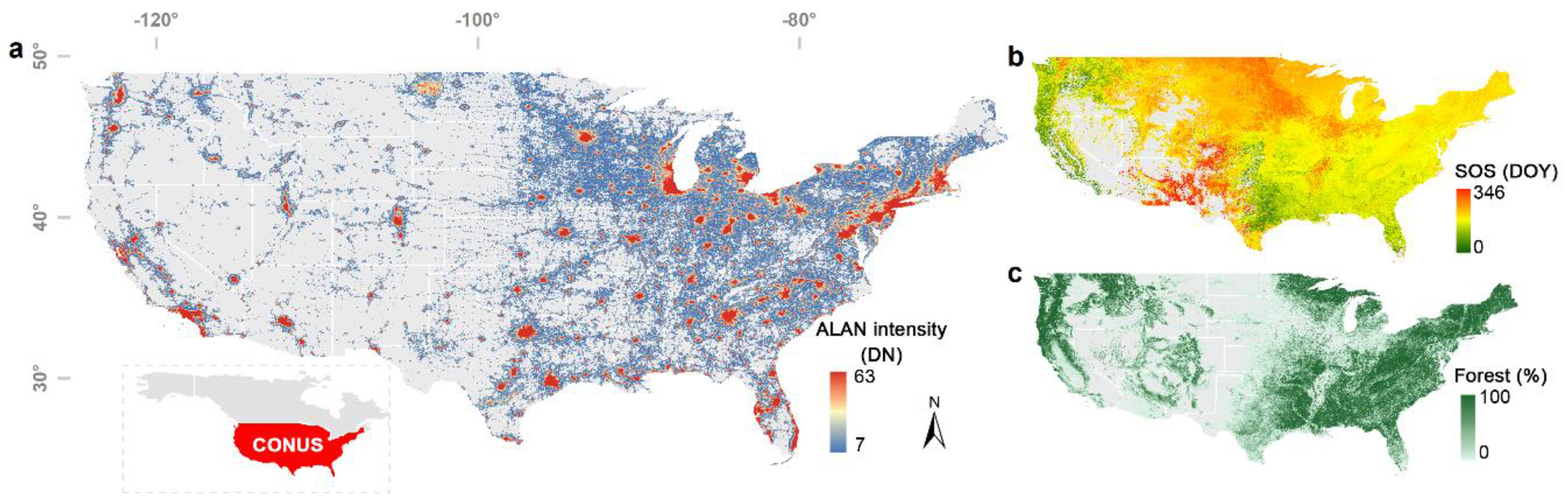
After excluding other covariant factors, our results overall suggest a statistically negative partial correlation (Wilcoxon signed-rank test, p < 0.001; Figure 2) between SOS and ALAN with an RALAN value of −0.19 (median, similarly hereinafter). It indicates that the occurrence and increase of ALAN would advance satellite-based spring phenology (i.e., SOS). A high variation in RALAN was observed (standard deviation = 0.28), ranging from −1 to 0.63 (excluding outliers). For the majority of pixels (71.7%), higher ALAN was associated with an advanced SOS with an RALAN− of −0.30. By comparison, only 28.3% of pixels showed a delay effect on SOS, whilst the magnitude of the delay effect (RALAN+ = 0.17) was significantly weaker than that of advancing effect (p < 0.001).
Preseason air temperature is well-acknowledged for its foremost control on spring phenology events, including SOS [48]. As expected, the overall phenological response to ALAN was weaker than to preseason temperature (RT = −0.60). The advancing effect of a warming temperature was observed in the bulk of pixels (91.3%) and had a much closer association with SOS (RT− = −0.61) than RALAN, whereas their counterparts, i.e., RT+ and RALAN+ did not differ greatly in correlation magnitude (RT+ = 0.14). This finding suggests that, albeit with an overall advancing effect, ALAN is a minor cue of SOS and its capability in influencing spring phenology is relatively weaker than temperature.
Our findings are largely consistent with previous studies based on field observations [24,25,49] and manipulated experiments [18,50,51], which highlight the association between ALAN and SOS but also a great diversity among species and sites. For example, by leveraging field phenology observations and ALAN intensity measured by DMSP-OLS data, it was found a 7.5 days advance in budburst date of tree species in response to per unit of ALAN increase [49]. By comparison, a large variation, from four days earlier to 12 days later, was observed in the flowering date of grass species exposed to LED lighting in a semi-natural environment [18]. The differences between our findings and others can be resulted from the differences in research methodologies, such as the data used (e.g., satellite-derived phenology vs. field observation-based phenology), research objects (e.g., forest vs. grass species), and research settings (e.g., real-world setting vs. environment-controlled condition).
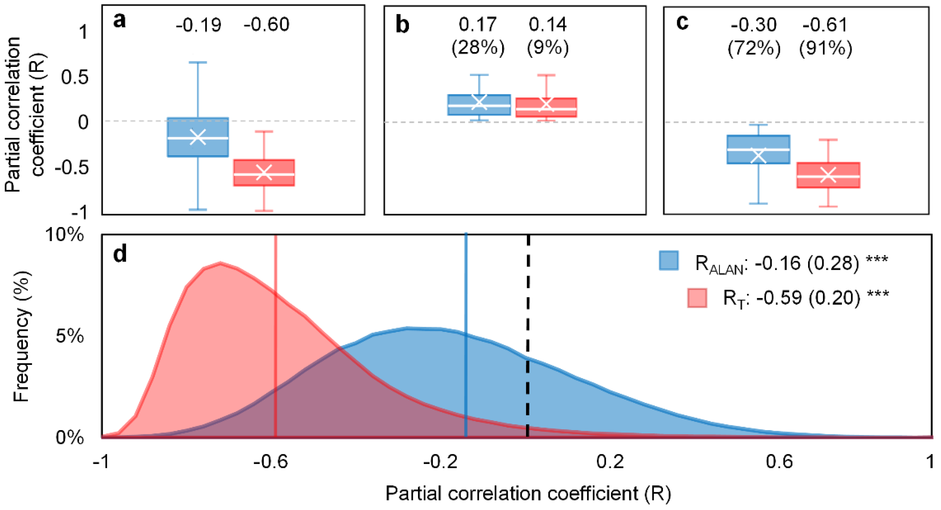
Potential bias can be incurred by DMSP-OLS data for its representativeness of the real night sky brightness. What night light satellite detects is mainly the zenith-directed light emissions at cloud-free nights [52], such that the light scattered into the night sky (e.g., skyglow) can be underestimated. To examine this issue, we compared DMSP-OLS data with a night sky luminance map calibrated by light pollution propagation model and satellite and ground measurements [17]. A moderate correlation between DMSP-OLS and night sky luminance was found (R2 = 0.63, p < 0.001; Figure 3), suggesting the appropriateness of using DMSP-OLS to present ALAN intensity.
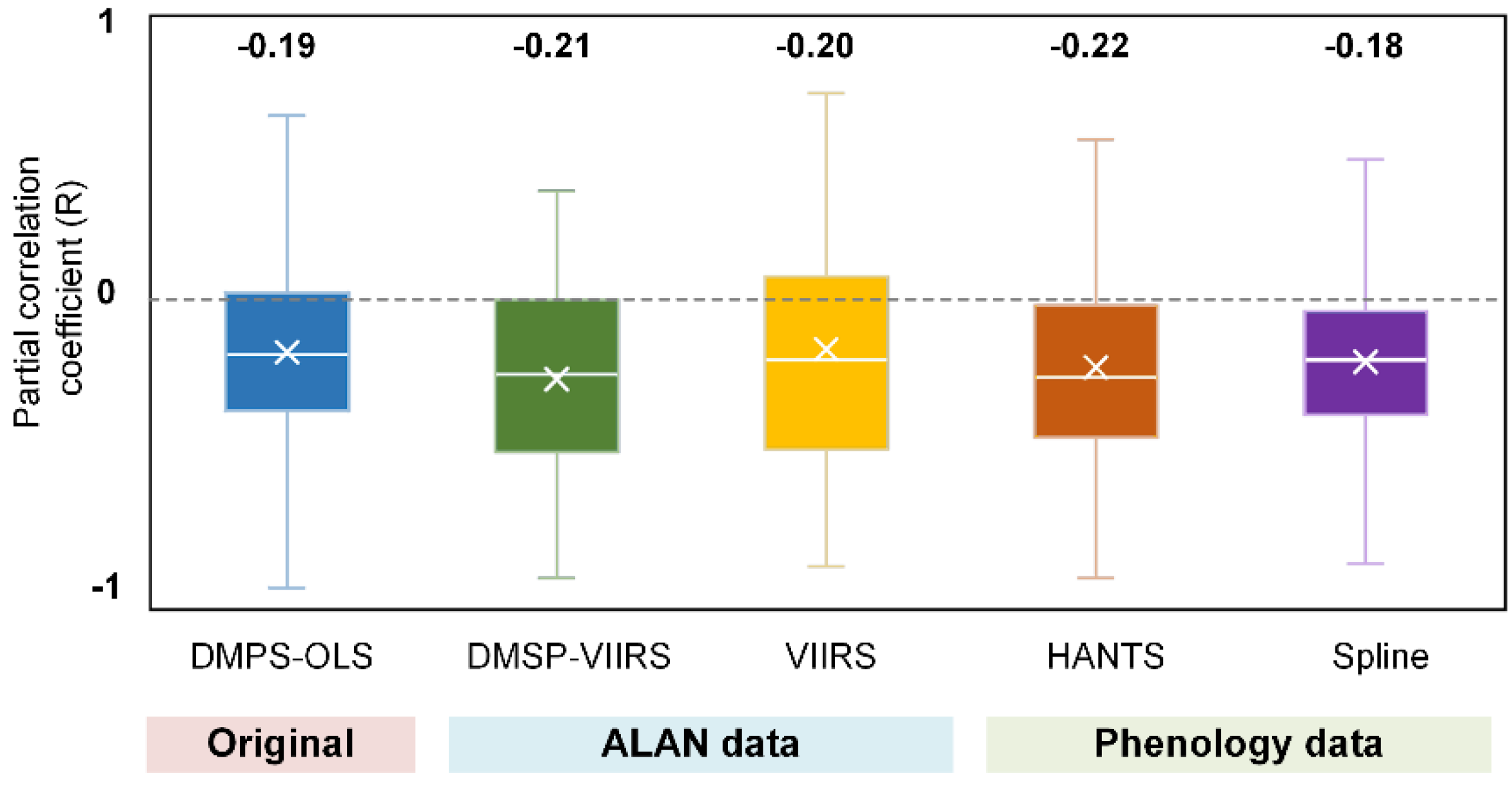
Besides, systematic errors of DMSP-OLS data and the uncertainties in phenology data extracted from MCQ12Q2 and the intercalibration process of DMSP-OLS data may also influence the validity our results. We thus applied the same analysis to two additional ALAN maps from DMSP-VIIRS data (2001–2018) and VIIRS data (2012–2018) and two additional phenology estimates using HANTS-maximum and spline-midpoint methods. As demonstrated in Figure 4, results derived from four comparative groups were generally consistent to DMSP-OLS based result, underpinning the robustness of our results. Among these, using the phenology data estimated by HANTS-Maximum method yielded the highest RALAN value (−0.22), while replacing DMSP-OLS with VIIRS data for ALAN mapping produced the highest variation (standard deviation = 0.37).
It should be noted that only DMSP-OLS was used for the subsequently analysis, instead of DMSP-VIIRS data or VIIRS data, because of three concerns:
- (1)
- Data availability. Subjected to the availability of NTL data and the corresponding phenology and climate data, VIIRS data were only available for 6.12 ± 1.17 yr. for each pixel, while DMSP-OLS data is available for 12.2 ± 3.28 yr. The partial correlation analysis was vulnerable to the impact of short-term observations [53].
- (2)
- Overpass time. DMSP-OLS (7:30 p.m.) has a more ideal overpass time than VIIRS (1:30 a.m.) because the peak lighting hour is approximately from sunset to 22:00 p.m. [54]. Using DMSP-OLS data enables us to evaluate the phenological response to ALAN when most artificial lights are on.
- (3)
- Despite a longer temporal coverage of DMSP-VIIRS data, the uncertainties of cross-sensor calibration algorithm to generate DMSP-VIIRS data may propagate to and confound our analysis [55].
3.2. Divergent Spatial Pattern of the Phenological Impact of ALAN
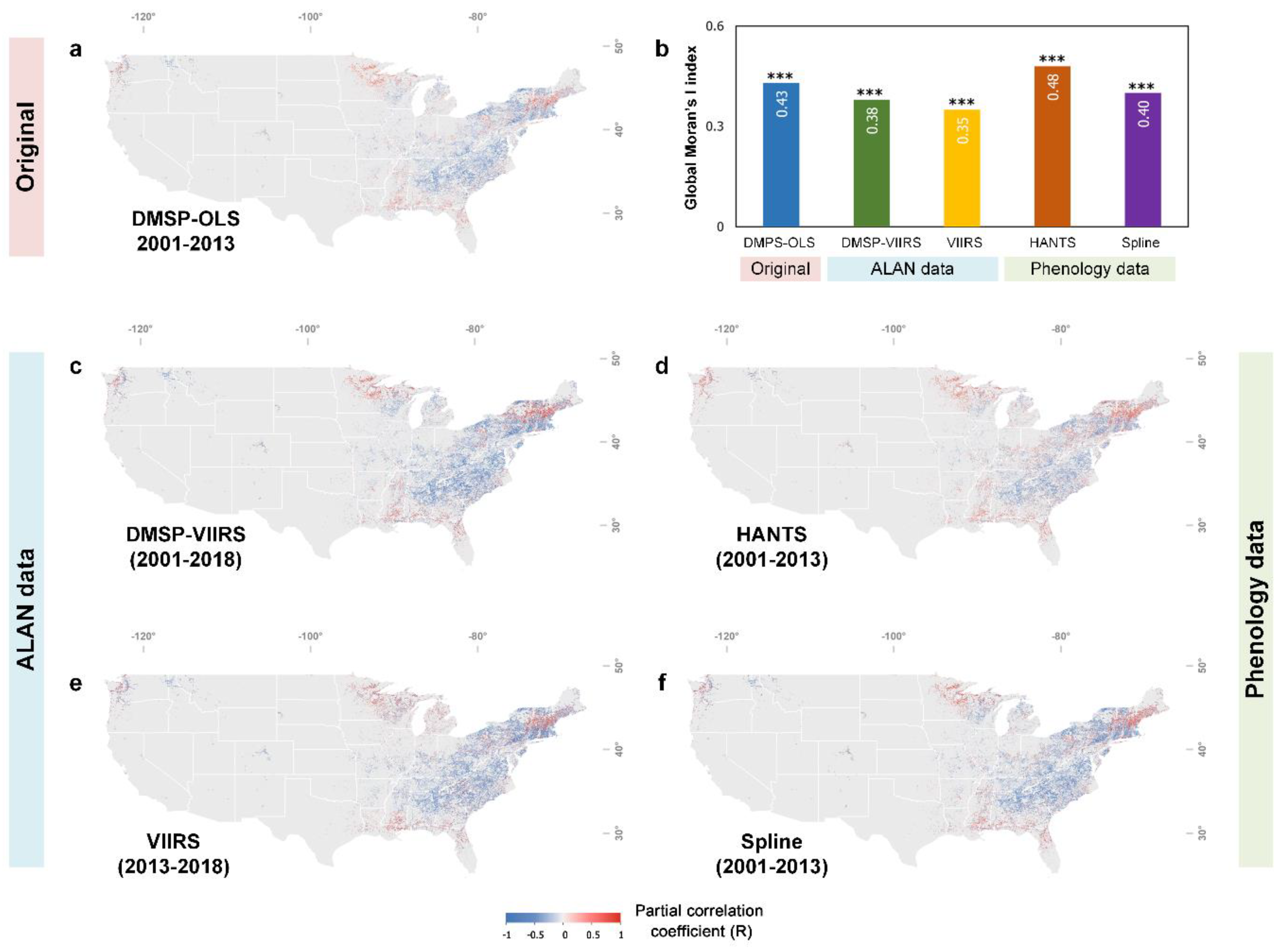
Satellite data products allow us to look into the spatial pattern of the phenological impact of ALAN. Figure 5a demonstrates the spatial distribution of RALAN over the CONUS. Since most of the forest and human settlements are located in the east part of the CONUS, our results are thus mainly distributed in the entire Northeast, as well as the east part of the Midwest and South. Comparing RALAN+ and RALAN− pixels, we found a noticeably clustered spatial pattern. This pattern was corroborated by global Moran’s I test (Moran’s I index = 0.43, p < 0.001), a spatial autocorrelation measurement, indicating the distribution of RALAN+ and RALAN− pixels was more spatially clustered other than randomly scattered (Figure 5b). As illustrated by latitudinal transects, most of RALAN− pixels were clustered between 30°N and 45°N, while RALAN+ pixels mainly spread over low (<30°N) and high (>45°N) latitude regions (Figure 6b). Similar results were found in the four comparative analysis with different input datasets (Figure 5c–f).
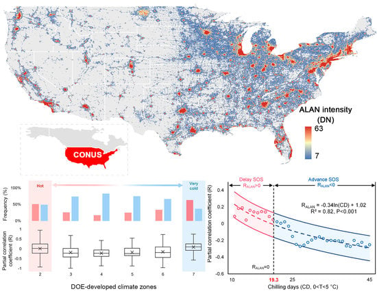
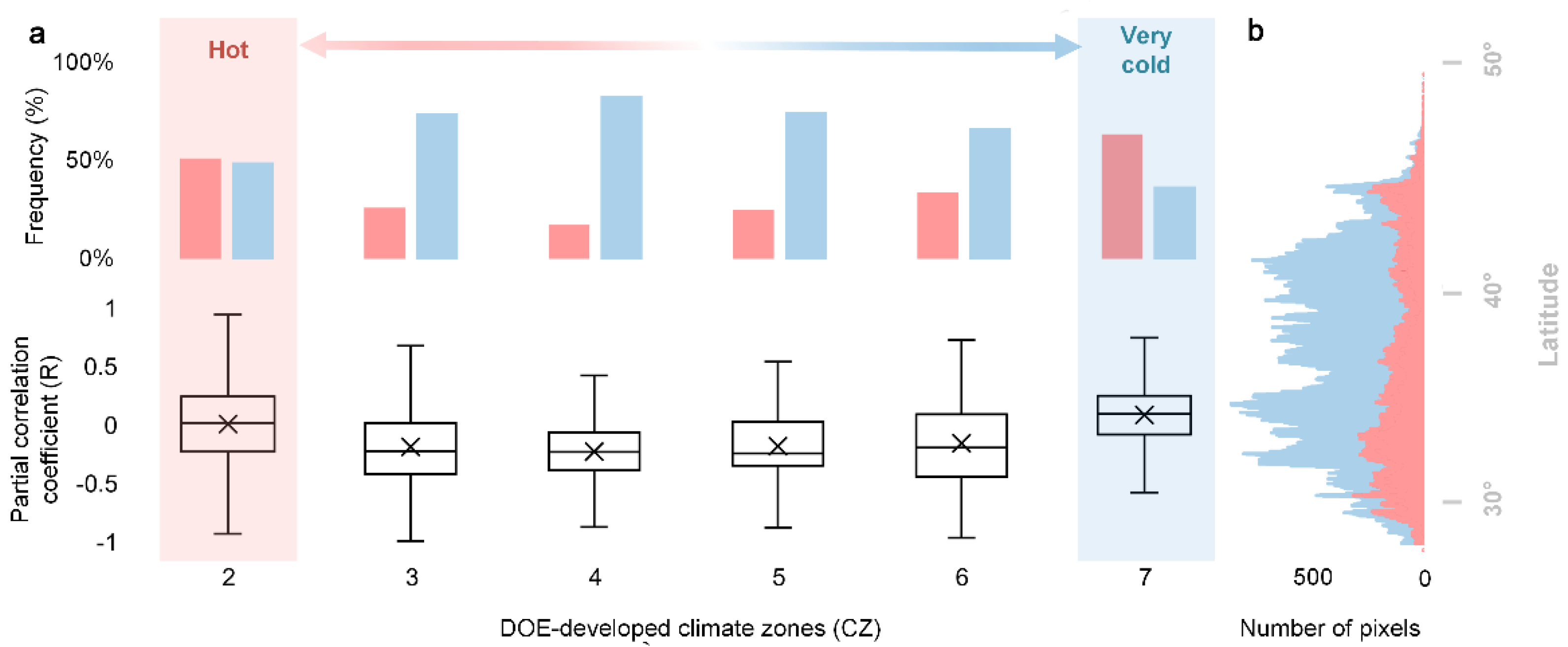
Furthermore, we grouped RALAN into climate zones developed by the United States Department of Energy (DOE-developed climate zones), which categorize the United States into 8 climate regimes, from the hottest climate zone 1 (CZ1) to the coldest climate zone 8 (CZ8), according to regional temperature characters [56]. It further demonstrated the spatial pattern of ALAN’s impact on SOS and revealed its linkage to regional temperature gradient (Figure 6a). Specifically, for climatically moderate regions (CZ3 to CZ6), like Virginia, ALAN tended to advance SOS, where RALAN ranged from −0.13 (CZ6) to −0.24 (CZ4). There was a dominant proportion of RALAN− pixels (74.5 ± 0.06%) over RALAN+ pixels (25.5 ± 0.06%). In stark contrast, hot regions (CZ2), such as Mississippi, Florida, southern Georgia and Atlanta, showed an insignificant effect of ALAN (p = 0.41) with an approximately equal amount of RALAN+ (51.0%) and RALAN− (49.0%) pixels. For very cold regions (CZ7), like New Hampshire, Vermont, Minnesota, and eastern Wisconsin, the impact of ALAN was even inversed to cause a delayed SOS (p < 0.001), whilst the number of RALAN+ pixels (63.3%) surpassed RALAN− pixels (36.7%). These above-mentioned phenomena underlined a spatially divergent response of SOS to ALAN between climatically moderate regions (CZ3 to CZ6) and hot (CZ2)/very cold regions (CZ7).
3.3. Urban. vs. Non-Urban. Area
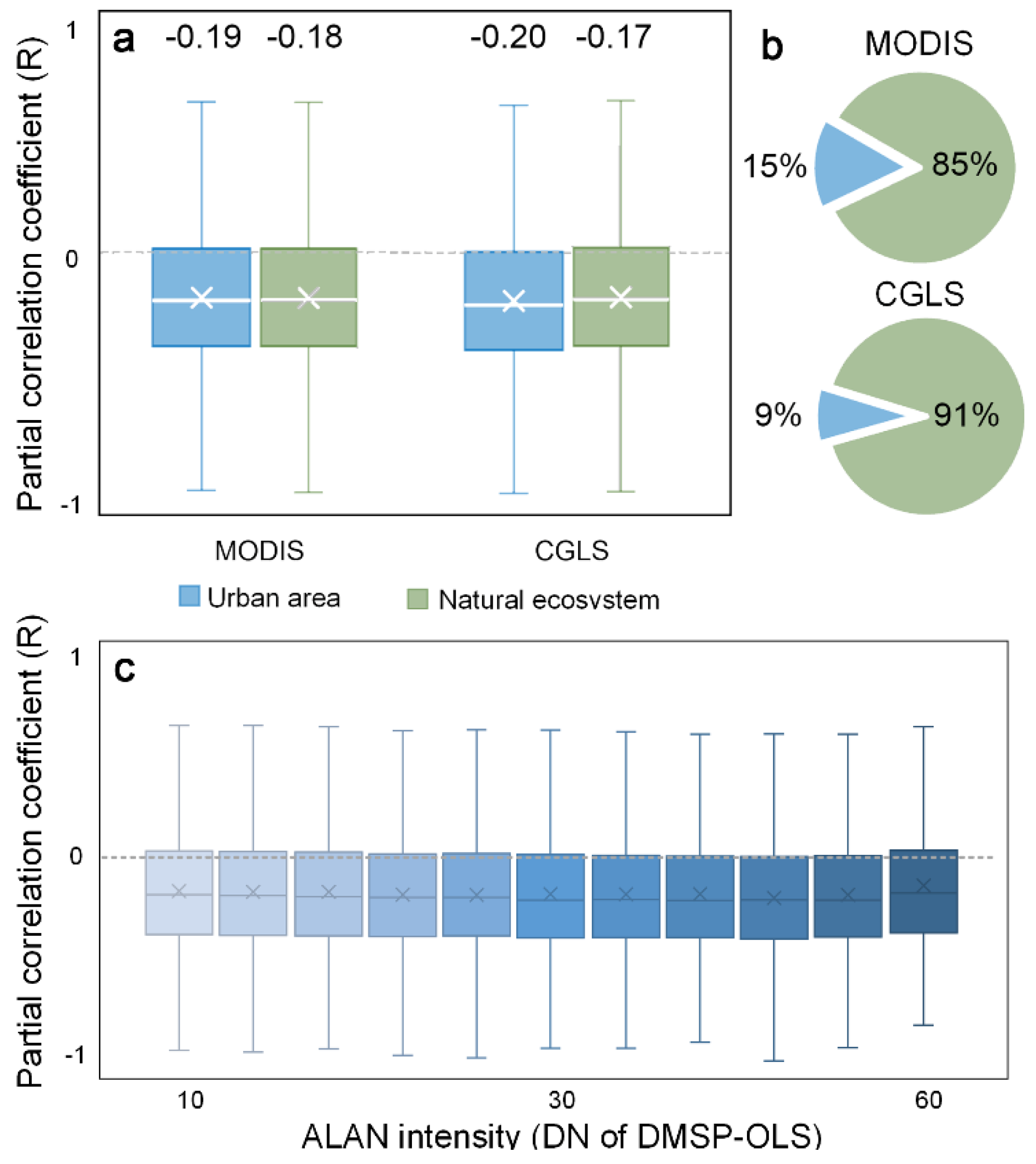
In addition to the regional spatial pattern, we probed into how ALAN’s effect varied over urban areas and non-urban natural ecosystems. We classified our study area into urban areas and nature ecosystem using MODIS and CGLS land cover map products, separately, and compared the corresponding RALAN values. Considering that ALAN is more intensive in urban areas, we expected SOS had a stronger response to ALAN in urban areas than natural ecosystems. Surprisingly, only slight RALAN differences were observed between urban areas (MODIS: −0.180; CGLS: −0.199) and nature ecosystems (MODIS: −0.174; CGLS: −0.173) (Figure 7a). We also found that RALAN values remained at a similar level regardless of the baseline ALAN magnitude (Figure 7c). It suggests that, despite a relatively low magnitude of the ALAN encroaching into natural ecosystems, it is enough to trigger phenology changes similar to the effect in brightly-lit urban areas. This phenomenon may be because light is mainly served as an information source, rather than an energy resource, for photoperiodism related processes [57]. Organisms use the changes in the natural light cycles as indicators of time and place and to detect changes in environment [58]. Hence, even though ALAN is at low intensities and/or of short duration in natural ecosystems, it is still able to incur marked phenological effect [42,57].
4. Discussions
4.1. Mechanisms of the Divergent Spatial Pattern
Our study found a spatially divergent pattern in the phenological response of ALAN between climatically moderate and hot/very cold regions, respectively. To our knowledge, this study is for the first time to reveal such a spatial pattern, whilst there is barely any well-established theory to explain the possible causes of it. Here, we proposed three potential and non-exclusive explanations for the phenomenon.
4.1.1. The Interplay among Chilling, Forcing and Photoperiod
We first attribute the advancing effect of ALAN in climatically moderate regions to the interplay among the intensity and length of winter temperature (chilling), warm spring temperature (forcing), and photoperiod (daylength). Photoperiod exerts an impact on phenology by influencing dormancy release through its sophisticated interaction with other environmental cues [46]. Studies utilizing in situ observations and environment-controlled experiments have found that insufficient winter chilling (or spring forcing) can be compensated, at least partly, by a longer photoperiod and additional forcing (or chilling) [10,11]. As a result, this interplay mechanism between photoperiod and the other two environmental cues, i.e., chilling and forcing, leads to an earlier SOS when a longer photoperiod occurs [59]. The ALAN lights up the night sky after sunset, and thus it could be regarded as a factor prolonging the original photoperiod (daylength) [18]. Note that in this study what we measured was how SOS responded to the change in ALAN intensity rather than the change of the duration that plants perceived ALAN. Due to data unavailability, it is currently impossible to measure the duration that the plants are exposed to ALAN during the night at a large scale [41]. We assume that if a pixel has a higher ALAN intensity, it is likely to indicate a longer overall photoperiod of the plants therein. The rationale behind this assumption is that within a 1 × 1 km pixel, artificial light from a brighter source can spread and penetrate to a larger extent [60]. Therefore, a higher proportion of plants within the pixel will be exposed to ALAN and experience a prolonged photoperiod. Based on our assumption and the aforementioned interplay mechanism, we ascribe the advancing effect to the prolonged photoperiod induced by ALAN increase.
4.1.2. Chilling Insufficient
Second, explanation for ALAN’s delay effect in hot and very cold regions could be rather complicated. As mentioned above, a longer photoperiod and additional forcing compensate for insufficient chilling, resulting in an earlier SOS. Nevertheless, the interplay mechanism has been reported to be non-linear [53]—that is, excessive chilling insufficiency may outweigh the compensating capacity of a longer photoperiod and additional forcing, consequently constraining the advancing effect on SOS and even turning it into the opposite [9,30,61]. To test whether this “chilling insufficiency” theory held true for the relationship between ALAN and SOS, we calculated the number of effective chilling days (CD, 0 < T < 5 °C) of each pixel and grouped them into DOE-developed climate zones. Our result demonstrated that hot region (CZ2, 20.5 ± 4.3 days) and very cold region (CZ7, 21.7 ± 3.1 days) had fewer number of chilling days than climatically moderate regions (CZ3 to CZ6, 30.7 ± 5.1 days, p < 0.001; Figure 8, red bar). It implies that hot and very cold regions are inclined to suffer more from chilling insufficiency than climatically moderate regions. The insufficient chilling can be caused by the following reasons: in lower temperate and subtropical regions like CZ2, global warming has resulted in warm winters in recent years, making it even hard to meet the chilling requirement [53,62]. For very cold regions (CZ7), the winter temperature is far below the effective range for fulfilling the chilling requirement (0 < T < 5 °C) [47] and the low temperature may also pose extra stress to the ALAN–SOS relationship (Figure 8, blue bar) [63].
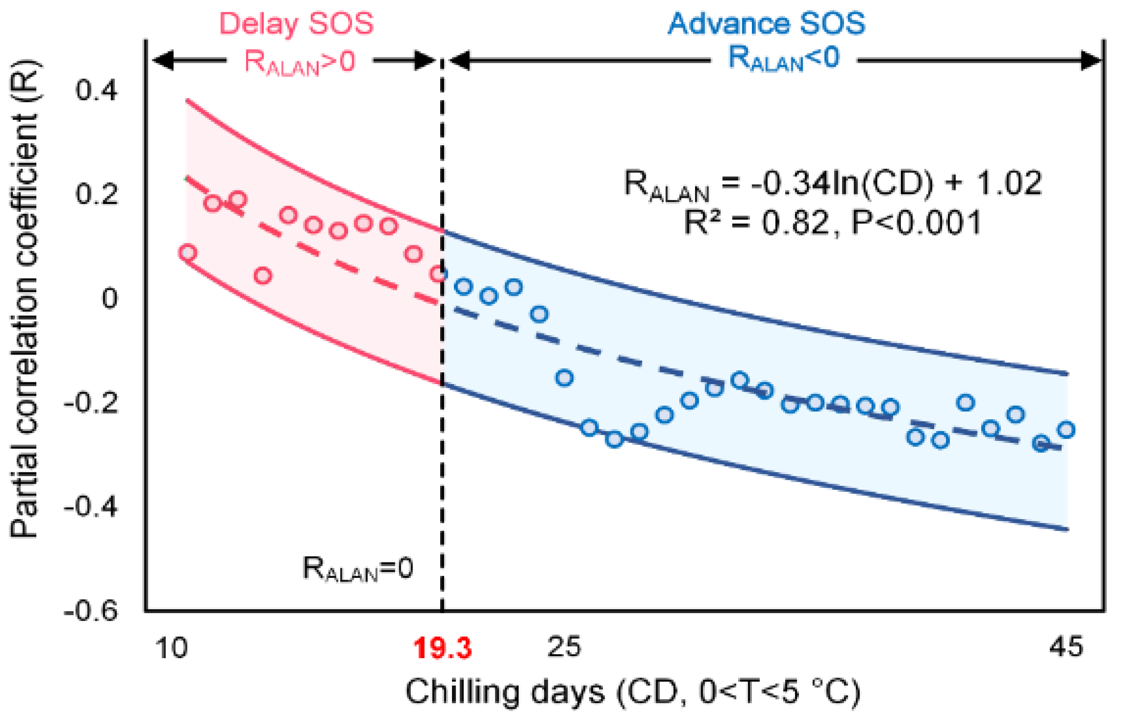
Furthermore, we calculated the RALAN of each CD group at a 1-CD interval and explored the relationship between CD and RALAN by linear regression analysis (Figure 9). The logarithmic transformed CD (ln(CD)) and RALAN was found negatively related with a slope of −0.35 (R2 = 0.82, p < 0.001). For most pixels whose CD value exceeds 19.3 days, the sign of RALAN remained negative, while RALAN changed into a positive sign when CD was below this threshold. This phenomenon suggests that the advancing effect of ALAN only functions on the premise that chilling requirement is met, at least to a certain degree. When CD is below a certain threshold, the chilling insufficiency will offset the ALAN-induced SOS advancement and lead to an insignificant or reversed ALAN-SOS relationship. Comparing the sign of RT (RT+ and RT−) for pixels showing a delay effect of ALAN (RALAN+), it turned out that a higher temperature could still result in an earlier SOS for more than 98% of RALAN+ pixels. Again, it shows that ALAN is not such a primary phenology driver as preseason temperature and its impact on SOS is sensitive to chilling requirement, while the impact of temperature is more tolerant against chilling insufficiency. These findings supported our hypothesis that the delay effect of ALAN could be incurred by insufficiency of winter chilling.
4.1.3. Differences in Species’ Life Strategies
The difference in species life strategies can also play a role in inducing the divergent response to ALAN. Studies have revealed that early successional species, such as hazel, poplars and birch, adopt a riskier life strategy to make the best use of growing resources and to maximize the growing season [7,64]. The start of the growing season of these species only relies on one or two key phenology drivers, i.e., forcing and/or chilling, and is less sensitive to other minor cues like ALAN and photoperiod. However, late successional species have evolved to be more conservative against environment changes to hinder early growth in unfavorable conditions (e.g., warm winter with high frost risk). These species have a strict requirement for environment cues and therefore can be both temperature-dependent and ALAN-dependent (photoperiod-dependent) [10,59]. In addition, tree cutting experiments reported that the leaf-out date of species from high latitudes is independent of photoperiod [5]. Spring phenology events are mainly driven by chilling and forcing rather than photoperiod in regions with long winter (like regions of CZ7 in this study). On the contrary, species originated from climatically moderate regions (like CZ3 to CZ6) may rely on additional information from photoperiodism [65].
4.2. Implications
Our study provides empirical evidence about how spring phenology is noticeably influenced by ALAN encroachment. We showed that ALAN tended to advance SOS, and this effect was statistically significant but relatively weaker than the effect caused by preseason temperature. We found a spatially divergent pattern of the effect in climatically moderate regions and hot/very cold regions and attributed it to:
- (1)
- the interplay among forcing, chilling and photoperiod;
- (2)
- chilling insufficiency, as we found the phenological impact of ALAN was sensitive to the accumulated chilling days;
- (3)
- the differences in life strategies of species. The results have an implication to understand the interaction mechanism between phenology shifts and environmental stimuli. It helps to better forecast how phenology will be influenced by and feedback to the warming climate and the environment being modified by human activities. Revealing the spatial variation of the impact of ALAN and its linkage to other environmental cues of phenology is a complement to in situ observation and experiment-based studies. Our results imply that previous studies about daylength and photoperiod may underestimate its actual potential in shifting phenology, especially for places where ALAN is prevailing. Hence, the long-lasting controversy on how ALAN (or photoperiod) affects phenology can be a result of not taking ALAN into consideration (for studies related to photoperiod) and/or the divergent spatial pattern of the ALAN-SOS relationship (for studies related to photoperiod and ALAN). We foresee a promising potential in improving the existing temperature-photoperiod based phenology models by incorporating the impact of ALAN [66].
Furthermore, our result showed that urban areas and natural ecosystems were subject to similar magnitude of phenological impact from ALAN, although the ALAN intensity in natural ecosystems was much lower than that in urban areas. This finding calls for further awareness of the phenological and ecological impact of ALAN in natural ecosystems because most of the areas under the influence of ALAN are natural ecosystems rather than human-dominated regions. In our case, about 87.7% of areas affected by ALAN were natural land, whereas urban areas only accounted for a small percentage (12.3%) of ALAN-affected areas (Figure 7b). On a global scale, human settlement only occupies 3% of the Earth’s land surface, but the resulting influences caused by ALAN will be rather far-reaching beyond urban footprint, where about 20% of the Earth’s surface under ALAN’s influence is natural land. Such widespread influence of ALAN is projected to continue to exacerbate in terms of both magnitude (1.8% yr−1) and extent (2.2% yr−1) [52]. Hence, it is imperative to propel lighting regulation and a better lighting design to reduce unnecessary light emission in urban areas and to minimize light pollution encroachment in natural ecosystems.
4.3. Limitations
The following issues should be noted and require further scrutiny in future studies. First, our results are based on coarse resolution satellite images, for which the mix pixel issue is inevitable. The phenology data extracted from long-term field observations can be further used. It can also help to explore the potential impact of species and taxa on the ALAN-phenology interaction. However, field phenology observation data were not considered for this study due to their limited temporal availability. For example, the species-site combination of the USA National Phenology Network data (USA-NPN; 2009), on average, only has 2.01 ± 1.87 yr. of valid observations. Less than 5% of the combinations have more than 6-year observations. Using short-term observations will bias our results by making the partial correlation analysis sensitive to the start and end values [53]. In future studies, it would be beneficial to incorporate long-term satellite and field phenology observations, together with other possible phenology cues (e.g., urban heat island effects), to have a more elaborated investigation into the phenology changes induced by human activities.
Second, it is challenging thus far to measure the long-term sky brightness changes at a large spatial scale. Even though a good correlation is found between ALAN intensity derived from DMSP-OLS and night sky brightness, satellite-based ALAN intensity inevitably underestimates what is actually perceived by plants. Likewise, at this moment, there are barely any data that can provide temporally exhaustive information about the duration of ALAN throughout the night. Due to this limitation, we are only able to analyze the association between ALAN and SOS based on the assumption that a higher ALAN intensity will lead to a longer ALAN duration. These issues could be addressed when more data sets become available, e.g., night light satellite with a short revisit time or a geostationary orbit [67,68].
Third, in our analysis chilling days were calculated as the number of days with temperature between 0 and 5 °C, which is a commonly-adopted approach [47,69]. A recent study using in-situ phenology records of 30 perennials [70], however, found that using the temperature between 0 and 5 °C was an invalid method to calculate chilling days, because it could not reflect the negative relationship between chilling days and heat requirement. Instead, temperature below 5 °C is a more suitable way. It is an issue worthwhile further investigation and validation since it is closely linked with the explanation of causes of the spatial divergent response of SOS to ALAN.
5. Conclusions
The natural cycle of light, as one of the key components organizing the ecosystem, has been dramatically disrupted by the sharp increase and expansion of artificial light at night due to global urbanization. This study leveraged nighttime light remote sensing images and satellite-based phenology data to explore the phenological responses of ALAN, reveal its relation to space and other environmental cues, and explain the underlying mechanisms. We shed spatially explicit insights on how the start date of the growing season (SOS) of plant was affected by ALAN, and found that ALAN generally tended to advance SOS (RALAN = −0.19). We revealed that the effect had a spatially divergent pattern between climatically moderate regions and very hot/cold regions. Further analysis showed the divergent pattern was mainly attributable to the high sensitivity to chilling insufficiency, while the interplay among chilling, forcing and photoperiod and the difference in species life strategies also played a role. Our findings not only evoke further awareness of the phenological and ecological impacts of artificial light at night, but help us to better understand how phenology will be influenced by and feedback to the continuously changing climate and the environment being modified by human activities.
Supplementary Materials
The following are available online at https://0-www-mdpi-com.brum.beds.ac.uk/2072-4292/13/3/399/s1, Figure S1: Partial correlation analysis with different forest fraction threshold from 40% to 80% with a 10% interval.
Author Contributions
Conceptualization, Q.Z.; methodology, Q.Z.; visualization, Q.Z.; writing original draft, Q.Z.; writing-review and editing, Q.Z., H.C.T., and L.P.K.; supervision, L.P.K.; funding acquisition, L.P.K. All authors have read and agreed to the published version of the manuscript.
Funding
This research is supported by the National Research Foundation, Singapore, under its NRF Returning Singaporean Scientists Scheme (NRF-RSS2019-007).
Institutional Review Board Statement
Not applicable.
Informed Consent Statement
Not applicable.
Data Availability Statement
The datasets used in this study can be accessed either via Google Earth Engine or the linked provided in the text.
Acknowledgments
The authors appreciate the reviewers and the editor for their constructive comments and suggestions.
Conflicts of Interest
The authors declare no conflict of interest.
References
- Richardson, A.D.; Keenan, T.F.; Migliavacca, M.; Ryu, Y.; Sonnentag, O.; Toomey, M. Climate change, phenology, and phenological control of vegetation feedbacks to the climate system. Agr. Forest Meteorol. 2013, 169, 156–173. [Google Scholar] [CrossRef]
- Cook, B.I.; Wolkovich, E.M.; Parmesan, C. Divergent responses to spring and winter warming drive community level flowering trends. Proc. Natl. Acad. Sci. USA 2012, 109, 9000–9005. [Google Scholar] [CrossRef] [PubMed] [Green Version]
- Menzel, A.; Sparks, T.H.; Estrella, N.; Koch, E.; Aasa, A.; Ahas, R.; Alm-Kübler, K.; Bissolli, P.; Braslavská, O.g.; Briede, A. European phenological response to climate change matches the warming pattern. Global Chang. Biol. 2006, 12, 1969–1976. [Google Scholar] [CrossRef]
- Xie, Y.; Wang, X.; Silander, J.A., Jr. Deciduous forest responses to temperature, precipitation, and drought imply complex climate change impacts. Proc. Natl. Acad. Sci. USA 2015, 112, 13585–13590. [Google Scholar] [CrossRef] [PubMed] [Green Version]
- Zohner, C.M.; Benito, B.M.; Svenning, J.-C.; Renner, S.S. Day length unlikely to constrain climate-driven shifts in leaf-out times of northern woody plants. Nature Clim. Chang. 2016, 6, 1120–1123. [Google Scholar] [CrossRef]
- Penuelas, J.; Rutishauser, T.; Filella, I. Ecology. Phenology feedbacks on climate change. Science 2009, 324, 887–888. [Google Scholar] [CrossRef] [PubMed] [Green Version]
- Korner, C.; Basler, D. Plant science. Phenology under global warming. Science 2010, 327, 1461–1462. [Google Scholar] [CrossRef]
- Cleland, E.E.; Chuine, I.; Menzel, A.; Mooney, H.A.; Schwartz, M.D. Shifting plant phenology in response to global change. Trends Ecol. Evol. 2007, 22, 357–365. [Google Scholar] [CrossRef]
- Laube, J.; Sparks, T.H.; Estrella, N.; Hofler, J.; Ankerst, D.P.; Menzel, A. Chilling outweighs photoperiod in preventing precocious spring development. Global Chang. Biol. 2014, 20, 170–182. [Google Scholar] [CrossRef]
- Way, D.A.; Montgomery, R.A. Photoperiod constraints on tree phenology, performance and migration in a warming world. Plant. Cell Environ. 2015, 38, 1725–1736. [Google Scholar] [CrossRef]
- Flynn, D.F.B.; Wolkovich, E.M. Temperature and photoperiod drive spring phenology across all species in a temperate forest community. New Phytol. 2018, 219, 1353–1362. [Google Scholar] [CrossRef] [PubMed] [Green Version]
- Torres, D.; Tidau, S.; Jenkins, S.; Davies, T. Artificial skyglow disrupts celestial migration at night. Curr. Biol. 2020, 30, R696–R697. [Google Scholar] [CrossRef] [PubMed]
- Gaston, K.J. Lighting up the nighttime. Science 2018, 362, 744–746. [Google Scholar] [CrossRef] [PubMed]
- Zheng, Q.; Weng, Q.; Huang, L.; Wang, K.; Deng, J.; Jiang, R.; Ye, Z.; Gan, M. A new source of multi-spectral high spatial resolution night-time light imagery—JL1-3B. Remote Sens. Environ. 2018, 215, 300–312. [Google Scholar] [CrossRef]
- Aubé, M.; Kocifaj, M.; Zamorano, J.; Lamphar, H.S.; de Miguel, A.S. The spectral amplification effect of clouds to the night sky radiance in Madrid. J. of Quant. Spectrosc. Radiat. Transf. 2016, 181, 11–23. [Google Scholar] [CrossRef]
- Jiang, W.; He, G.; Long, T.; Wang, C.; Ni, Y.; Ma, R. Assessing Light Pollution in China Based on Nighttime Light Imagery. Remote Sens. 2017, 9, 135. [Google Scholar] [CrossRef] [Green Version]
- Falchi, F.; Cinzano, P.; Duriscoe, D.; Kyba, C.C.; Elvidge, C.D.; Baugh, K.; Portnov, B.A.; Rybnikova, N.A.; Furgoni, R. The new world atlas of artificial night sky brightness. Sci. Adv. 2016, 2, e1600377. [Google Scholar] [CrossRef] [PubMed] [Green Version]
- Bennie, J.; Davies, T.W.; Cruse, D.; Bell, F.; Gaston, K.J. Artificial light at night alters grassland vegetation species composition and phenology. J. Appl. Ecol. 2018, 55, 442–450. [Google Scholar] [CrossRef] [Green Version]
- Ayalon, I.; de Barros Marangoni, L.F.; Benichou, J.I.C.; Avisar, D.; Levy, O. Red Sea corals under Artificial Light Pollution at Night (ALAN) undergo oxidative stress and photosynthetic impairment. Global Chang. Biol. 2019, 25, 4194–4207. [Google Scholar] [CrossRef] [PubMed] [Green Version]
- Bennie, J.; Davies, T.W.; Cruse, D.; Gaston, K.J. Ecological effects of artificial light at night on wild plants. J. Ecol. 2016, 104, 611–620. [Google Scholar] [CrossRef] [Green Version]
- Gaston, K.J.; Duffy, J.P.; Gaston, S.; Bennie, J.; Davies, T.W. Human alteration of natural light cycles: Causes and ecological consequences. Oecologia 2014, 176, 917–931. [Google Scholar] [CrossRef] [PubMed] [Green Version]
- Aubé, M.; Marseille, C.; Farkouh, A.; Dufour, A.; Simoneau, A.; Zamorano, J.; Roby, J.; Tapia, C. Mapping the Melatonin Suppression, Star Light and Induced Photosynthesis Indices with the LANcube. Remote Sens. 2020, 12, 3954. [Google Scholar] [CrossRef]
- Xue, X.; Lin, Y.; Zheng, Q.; Wang, K.; Zhang, J.; Deng, J.; Abubakar, G.A.; Gan, M. Mapping the fine-scale spatial pattern of artificial light pollution at night in urban environments from the perspective of bird habitats. Sci. Total Environ. 2020, 702. [Google Scholar] [CrossRef] [PubMed]
- Škvareninová, J.; Tuhárska, M.; Škvarenina, J.; Babálová, D.; Slobodníková, L.; Slobodník, B.; Středová, H.; Minďaš, J. Effects of light pollution on tree phenology in the urban environment. Morav. Geogr. Rep. 2017, 25, 282–290. [Google Scholar] [CrossRef] [Green Version]
- Massetti, L. Assessing the impact of street lighting on Platanus x acerifolia phenology. Urban. For. Urban. Gree. 2018, 34, 71–77. [Google Scholar] [CrossRef]
- Briggs, W.R. Physiology of plant responses to artificial lighting. Ecol. Conseq. Artif. Night Lighting 2006, 389–411. [Google Scholar]
- Chen, G.; Li, X.; Liu, X.; Chen, Y.; Liang, X.; Leng, J.; Xu, X.; Liao, W.; Qiu, Y.a.; Wu, Q.; et al. Global projections of future urban land expansion under shared socioeconomic pathways. Nat. Commun. 2020, 11. [Google Scholar] [CrossRef] [Green Version]
- Nagendra, H.; Bai, X.; Brondizio, E.S.; Lwasa, S. The urban south and the predicament of global sustainability. Nat. Sustain. 2018, 1, 341–349. [Google Scholar] [CrossRef]
- Gray, J.; Sulla-Menashe, D.; Friedl, M.A. User Guide to Collection 6 MODIS Land Cover Dynamics (MCD12Q2) Product; NASA EOSDIS Land Processes DAAC: Missoula, MT, USA, 2019. [Google Scholar]
- Meng, L.; Zhou, Y.; Li, X.; Asrar, G.R.; Mao, J.; Wanamaker, A.D.; Wang, Y. Divergent responses of spring phenology to daytime and nighttime warming. Agr. Forest Meteorol. 2020, 281. [Google Scholar] [CrossRef]
- Cong, N.; Wang, T.; Nan, H.; Ma, Y.; Wang, X.; Myneni, R.B.; Piao, S. Changes in satellite-derived spring vegetation green-up date and its linkage to climate in China from 1982 to 2010: A multimethod analysis. Global Chang. Biol. 2013, 19, 881–891. [Google Scholar] [CrossRef]
- Liu, Q.; Fu, Y.H.; Zeng, Z.; Huang, M.; Li, X.; Piao, S. Temperature, precipitation, and insolation effects on autumn vegetation phenology in temperate China. Global Chang. Biol. 2016, 22, 644–655. [Google Scholar] [CrossRef] [PubMed]
- Zhang, Q.; Seto, K.C. Mapping urbanization dynamics at regional and global scales using multi-temporal DMSP/OLS nighttime light data. Remote Sens. Environ. 2011, 115, 2320–2329. [Google Scholar] [CrossRef]
- Elvidge, C.D.; Ziskin, D.; Baugh, K.E.; Tuttle, B.T.; Ghosh, T.; Pack, D.W.; Erwin, E.H.; Zhizhin, M. A Fifteen Year Record of Global Natural Gas Flaring Derived from Satellite Data. Energies 2009, 2, 595–622. [Google Scholar] [CrossRef]
- Liu, Z.; He, C.; Zhang, Q.; Huang, Q.; Yang, Y. Extracting the dynamics of urban expansion in China using DMSP-OLS nighttime light data from 1992 to 2008. Landsc. Urban. Plan. 2012, 106, 62–72. [Google Scholar] [CrossRef]
- Zheng, Q.; Weng, Q.; Wang, K. Correcting the Pixel Blooming Effect (PiBE) of DMSP-OLS nighttime light imagery. Remote Sens. Environ. 2020, 240. [Google Scholar] [CrossRef]
- Sanchez de Miguel, A.; Kyba, C.C.M.; Zamorano, J.; Gallego, J.; Gaston, K.J. The nature of the diffuse light near cities detected in nighttime satellite imagery. Sci. Rep. 2020, 10. [Google Scholar] [CrossRef] [PubMed]
- Levin, N.; Kyba, C.C.M.; Zhang, Q.; de Miguel, A.S.; Roman, M.O.; Li, X.; Portnov, B.A.; Molthan, A.L.; Jechow, A.; Miller, S.D.; et al. Remote sensing of night lights: A review and an outlook for the future. Remote Sens. Environ. 2020, 237. [Google Scholar] [CrossRef]
- Zheng, Q.; Weng, Q.; Wang, K. Characterizing urban land changes of 30 global megacities using nighttime light time series stacks. ISPRS J. Photogramm. Remote Sens. 2021, 173, 10–23. [Google Scholar] [CrossRef]
- Li, X.; Zhou, Y.; Zhao, M.; Zhao, X. A harmonized global nighttime light dataset 1992–2018. Scientific data 2020, 7, 1–9. [Google Scholar] [CrossRef]
- Román, M.O.; Wang, Z.; Sun, Q.; Kalb, V.; Miller, S.D.; Molthan, A.; Schultz, L.; Bell, J.; Stokes, E.C.; Pandey, B.; et al. NASA’s Black Marble nighttime lights product suite. Remote Sens. Environ. 2018, 210, 113–143. [Google Scholar] [CrossRef]
- Smith, H. Light quality, photoperception, and plant strategy. Annu. Rev. Plant Physiol. 1982, 33, 481–518. [Google Scholar] [CrossRef]
- Wu, C.; Wang, X.; Wang, H.; Ciais, P.; Peñuelas, J.; Myneni, R.B.; Desai, A.R.; Gough, C.M.; Gonsamo, A.; Black, A.T.; et al. Contrasting responses of autumn-leaf senescence to daytime and night-time warming. Nat. Clim. Chang. 2018, 8, 1092–1096. [Google Scholar] [CrossRef] [Green Version]
- Sulla-Menashe, D.; Gray, J.M.; Abercrombie, S.P.; Friedl, M.A. Hierarchical mapping of annual global land cover 2001 to present: The MODIS Collection 6 Land Cover product. Remote Sens. Environ. 2019, 222, 183–194. [Google Scholar] [CrossRef]
- Piao, S.; Tan, J.; Chen, A.; Fu, Y.H.; Ciais, P.; Liu, Q.; Janssens, I.A.; Vicca, S.; Zeng, Z.; Jeong, S.J.; et al. Leaf onset in the northern hemisphere triggered by daytime temperature. Nat. Commun. 2015, 6, 6911. [Google Scholar] [CrossRef] [Green Version]
- Fu, Y.H.; Zhang, X.; Piao, S.; Hao, F.; Geng, X.; Vitasse, Y.; Zohner, C.; Penuelas, J.; Janssens, I.A. Daylength helps temperate deciduous trees to leaf-out at the optimal time. Global Chang. Biol. 2019, 25, 2410–2418. [Google Scholar] [CrossRef]
- Fu, Y.H.; Zhao, H.; Piao, S.; Peaucelle, M.; Peng, S.; Zhou, G.; Ciais, P.; Huang, M.; Menzel, A.; Penuelas, J.; et al. Declining global warming effects on the phenology of spring leaf unfolding. Nature 2015, 526, 104–107. [Google Scholar] [CrossRef] [Green Version]
- Piao, S.; Liu, Q.; Chen, A.; Janssens, I.A.; Fu, Y.; Dai, J.; Liu, L.; Lian, X.; Shen, M.; Zhu, X. Plant phenology and global climate change: Current progresses and challenges. Global Chang. Biol. 2019, 25, 1922–1940. [Google Scholar] [CrossRef]
- Ffrench-Constant, R.H.; Somers-Yeates, R.; Bennie, J.; Economou, T.; Hodgson, D.; Spalding, A.; McGregor, P.K. Light pollution is associated with earlier tree budburst across the United Kingdom. Proc. Biol. Sci. 2016, 283. [Google Scholar] [CrossRef]
- Ouzounis, T.; Rosenqvist, E.; Ottosen, C.-O. Spectral effects of artificial light on plant physiology and secondary metabolism: A review. Hortscience 2015, 50, 1128–1135. [Google Scholar] [CrossRef] [Green Version]
- Whitman, C.M.; Heins, R.D.; Cameron, A.C.; Carlson, W.H. Lamp type and irradiance level for daylength extensions influence flowering of Campanula carpaticaBlue Clips’, Coreopsis grandifloraEarly Sunrise’, and Coreopsis verticillataMoonbeam’. J. Am. Soc. Hortic. Sci. 1998, 123, 802–807. [Google Scholar] [CrossRef] [Green Version]
- Kyba, C.C.M.; Kuester, T.; Sanchez de Miguel, A.; Baugh, K.; Jechow, A.; Holker, F.; Bennie, J.; Elvidge, C.D.; Gaston, K.J.; Guanter, L. Artificially lit surface of Earth at night increasing in radiance and extent. Sci. Adv. 2017, 3, e1701528. [Google Scholar] [CrossRef] [PubMed] [Green Version]
- Wang, X.; Xiao, J.; Li, X.; Cheng, G.; Ma, M.; Zhu, G.; Altaf Arain, M.; Andrew Black, T.; Jassal, R.S. No trends in spring and autumn phenology during the global warming hiatus. Nat. Commun. 2019, 10, 2389. [Google Scholar] [CrossRef] [PubMed]
- Elvidge, C.; Baugh, K.; Zhizhin, M.; Hsu, F.-C. Why VIIRS data are superior to DMSP for mapping nighttime lights. Proc. Asia Pac. Adv. Netw 2013, 35, 62. [Google Scholar] [CrossRef] [Green Version]
- Zheng, Q.; Weng, Q.; Wang, K. Developing a new cross-sensor calibration model for DMSP-OLS and Suomi-NPP VIIRS night-light imageries. ISPRS J. Photogramm. Remote Sens. 2019, 153, 36–47. [Google Scholar] [CrossRef]
- Burleyson, C. 2012 IECC Climate Zones; Pacific Northwest National Laboratory 2; Pacific Northwest National Lab. (PNNL): Richland, WA, USA, 2020. [Google Scholar]
- Gaston, K.J.; Bennie, J.; Davies, T.W.; Hopkins, J. The ecological impacts of nighttime light pollution: A mechanistic appraisal. Biol Rev. Camb Philos Soc. 2013, 88, 912–927. [Google Scholar] [CrossRef]
- Neff, M.M.; Fankhauser, C.; Chory, J. Light: An indicator of time and place. Gene Dev. 2000, 14, 257–271. [Google Scholar]
- Basler, D.; Körner, C. Photoperiod sensitivity of bud burst in 14 temperate forest tree species. Agr. Forest Meteorol. 2012, 165, 73–81. [Google Scholar] [CrossRef]
- Kocifaj, M.; Solano-Lamphar, H.A.; Videen, G. Night-sky radiometry can revolutionize the characterization of light-pollution sources globally. Proc. Natl. Acad. Sci. USA 2019, 116, 7712–7717. [Google Scholar] [CrossRef] [Green Version]
- Wang, X.; Piao, S.; Ciais, P.; Li, J.; Friedlingstein, P.; Koven, C.; Chen, A. Spring temperature change and its implication in the change of vegetation growth in North America from 1982 to 2006. Proc. Natl. Acad. Sci. USA 2011, 108, 1240–1245. [Google Scholar] [CrossRef] [Green Version]
- Richardson, A.D.; Bailey, A.S.; Denny, E.G.; Martin, C.W.; O’Keefe, J. Phenology of a northern hardwood forest canopy. Global Chang. Biol. 2006, 12, 1174–1188. [Google Scholar] [CrossRef] [Green Version]
- Richardson, A.D.; Hufkens, K.; Milliman, T.; Aubrecht, D.M.; Furze, M.E.; Seyednasrollah, B.; Krassovski, M.B.; Latimer, J.M.; Nettles, W.R.; Heiderman, R.R.; et al. Ecosystem warming extends vegetation activity but heightens vulnerability to cold temperatures. Nature 2018, 560, 368–371. [Google Scholar] [CrossRef] [PubMed]
- Caffarra, A.; Donnelly, A. The ecological significance of phenology in four different tree species: Effects of light and temperature on bud burst. Int. J. Biometeorol. 2011, 55, 711–721. [Google Scholar] [CrossRef] [PubMed]
- Tiffney, B.; Manchester, S. The influence of physical environment on phytogeographic continuity and phylogeographic hypotheses in the Northern Hemisphere Tertiary. Int. J. Plant. Sci. 2001, 162, S3–S17. [Google Scholar] [CrossRef]
- Migliavacca, M.; Sonnentag, O.; Keenan, T.F.; Cescatti, A.; O’Keefe, J.; Richardson, A.D. On the uncertainty of phenological responses to climate change, and implications for a terrestrial biosphere model. Biogeosciences 2012, 9, 2063–2083. [Google Scholar] [CrossRef] [Green Version]
- Elvidge, C.D.; Cinzano, P.; Pettit, D.R.; Arvesen, J.; Sutton, P.; Small, C.; Nemani, R.; Longcore, T.; Rich, C.; Safran, J.; et al. The Nightsat mission concept. Int. J. Remote Sens. 2007, 28, 2645–2670. [Google Scholar] [CrossRef]
- Li, X.; Levin, N.; Xie, J.; Li, D. Monitoring hourly night-time light by an unmanned aerial vehicle and its implications to satellite remote sensing. Remote Sens. Environ. 2020, 247. [Google Scholar] [CrossRef]
- Peaucelle, M.; Janssens, I.A.; Stocker, B.D.; Descals Ferrando, A.; Fu, Y.H.; Molowny-Horas, R.; Ciais, P.; Penuelas, J. Spatial variance of spring phenology in temperate deciduous forests is constrained by background climatic conditions. Nat. Commun. 2019, 10, 5388. [Google Scholar] [CrossRef] [Green Version]
- Wang, H.; Wu, C.; Ciais, P.; Penuelas, J.; Dai, J.; Fu, Y.; Ge, Q. Overestimation of the effect of climatic warming on spring phenology due to misrepresentation of chilling. Nat. Commun. 2020, 11, 4945. [Google Scholar] [CrossRef]
Figure 1.
Artificial light at night (ALAN) intensity presented by DMSP–OLS nighttime light data in 2013 (a), the start date of the growing season (SOS) derived from MCD12Q2 product of 2013 (b) and forest fraction (c) of the conterminous United States (CONUS).
Figure 1.
Artificial light at night (ALAN) intensity presented by DMSP–OLS nighttime light data in 2013 (a), the start date of the growing season (SOS) derived from MCD12Q2 product of 2013 (b) and forest fraction (c) of the conterminous United States (CONUS).

Figure 2.
Phenological responses to ALAN (RALAN) and preseason temperature (RT) in CONUS during 2001–2013. The partial correlation coefficient of all pixels (RALAN and RT; (a), pixels with positive partial correlation coefficients (RALAN+ and RT+; (b), and pixels with negative partial correlation coefficients (RALAN− and RT−; (c). The box plots show the median (horizontal line) and mean (cross) values, 75th and 25th percentiles with upper and lower hinges, and 1.5× IQR with whiskers; Outliers are omitted for a clear demonstration. The median value and the corresponding percentage (in parentheses) of RALAN+/RALAN− and RT+/RT− pixels are provided. The frequency distribution of RALAN and RT (d). The colored vertical lines represent the mean RALAN and RT values with the standard deviation (in parentheses). *** indicates the significance level of the Wilcoxon signed-rank test (p < 0.001) under the null hypothesis that RALAN (or RT) equals 0.

Figure 3.
Linear regression of field observation based night sky brightness (mcd/m2) and satellite-based ALAN intensity (DN).
Figure 3.
Linear regression of field observation based night sky brightness (mcd/m2) and satellite-based ALAN intensity (DN).

Figure 4.
Comparison of RALAN among different datasets. Original: DMSP–OLS (ALAN) + MCD12Q2 (Phenology); ALAN data: DMSP–VIIRS and VIIRS (ALAN) + MCD12Q2 (Phenology); Phenology data: DMSP–OLS (ALAN) + HANTS–Maximum method and Spline–Midpoint method (Phenology). The median RALAN values are provided at the top.

Figure 5.
Spatial pattern of the phenological response to ALAN derived from the original and four additional comparative analysis (a,c–f). Global Moran’s I statistic (b). *** indicates the significance level of Global Moran’s I statistics (p < 0.001).
Figure 5.
Spatial pattern of the phenological response to ALAN derived from the original and four additional comparative analysis (a,c–f). Global Moran’s I statistic (b). *** indicates the significance level of Global Moran’s I statistics (p < 0.001).

Figure 6.
RALAN categorized by climate zones developed by the US Department of Energy (DOE–developed climate zones; (a)). The lower and upper panels present box plots of RALAN and the frequency distribution (%) of RALAN+ and RALAN− pixels of each climate zone (CZ), from hot (CZ2) to very cold (CZ7), respectively. The number of RALAN+ and RALAN− pixels along the latitudinal transect (b).

Figure 7.
Phenological impact of ALAN in urban areas and natural ecosystems. RALAN of urban areas and natural ecosystems (a). Fraction of urban areas and natural ecosystems. Urban areas and natural ecosystems are derived from MODIS and CGLS land cover map products, respectively (b). RALAN with different baseline ALAN intensity from 10 to 60 at a 5–DN interval (c).

Figure 8.
Relationship between DOE–developed climate zones and chilling requirement. The number of accumulated chilling days (0 < T < 5 °C; red bars) and accumulated days when air temperature (T) is below 5 °C (blue bars) for each climate zone.
Figure 8.
Relationship between DOE–developed climate zones and chilling requirement. The number of accumulated chilling days (0 < T < 5 °C; red bars) and accumulated days when air temperature (T) is below 5 °C (blue bars) for each climate zone.

Figure 9.
Relationship between RALAN and chilling days (CD). The circle presents the median RALAN values of each CD group at a 1–CD interval. The colored dash line is the fitted model with the upper and lower bounds indicating the 95% confidence interval, respectively; the vertical dash line is the CD threshold when RALAN equals 0.

Publisher’s Note: MDPI stays neutral with regard to jurisdictional claims in published maps and institutional affiliations. |
© 2021 by the authors. Licensee MDPI, Basel, Switzerland. This article is an open access article distributed under the terms and conditions of the Creative Commons Attribution (CC BY) license (http://creativecommons.org/licenses/by/4.0/).
Share and Cite
MDPI and ACS Style
Zheng, Q.; Teo, H.C.; Koh, L.P. Artificial Light at Night Advances Spring Phenology in the United States. Remote Sens. 2021, 13, 399. https://0-doi-org.brum.beds.ac.uk/10.3390/rs13030399
AMA Style
Zheng Q, Teo HC, Koh LP. Artificial Light at Night Advances Spring Phenology in the United States. Remote Sensing. 2021; 13(3):399. https://0-doi-org.brum.beds.ac.uk/10.3390/rs13030399
Chicago/Turabian StyleZheng, Qiming, Hoong Chen Teo, and Lian Pin Koh. 2021. "Artificial Light at Night Advances Spring Phenology in the United States" Remote Sensing 13, no. 3: 399. https://0-doi-org.brum.beds.ac.uk/10.3390/rs13030399
Note that from the first issue of 2016, this journal uses article numbers instead of page numbers. See further details here.