
Fast Hyper-Spectral Radiative Transfer Model Based on the Double Cluster Low-Streams Regression Method


Remote Sensing Technology Institute (IMF), German Aerospace Center (DLR), 82234 Oberpfaffenhofen, Germany
*
Author to whom correspondence should be addressed.
Remote Sens. 2021, 13(3), 434; https://0-doi-org.brum.beds.ac.uk/10.3390/rs13030434
Submission received: 28 December 2020
/
Revised: 18 January 2021
/
Accepted: 23 January 2021
/
Published: 27 January 2021
(This article belongs to the Special Issue Current Advances in Radiative Transfer Modeling for Satellite Optical Remote Sensing Applications)
Abstract
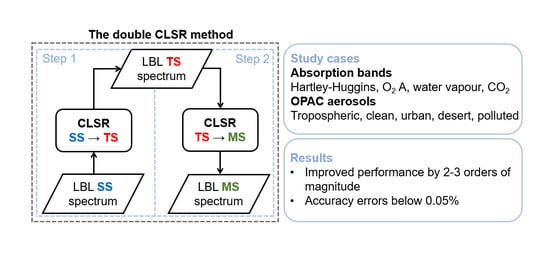
:Fast radiative transfer models (RTMs) are required to process a great amount of satellite-based atmospheric composition data. Specifically designed acceleration techniques can be incorporated in RTMs to simulate the reflected radiances with a fine spectral resolution, avoiding time-consuming computations on a fine resolution grid. In particular, in the cluster low-streams regression (CLSR) method, the computations on a fine resolution grid are performed by using the fast two-stream RTM, and then the spectra are corrected by using regression models between the two-stream and multi-stream RTMs. The performance enhancement due to such a scheme can be of about two orders of magnitude. In this paper, we consider a modification of the CLSR method (which is referred to as the double CLSR method), in which the single-scattering approximation is used for the computations on a fine resolution grid, while the two-stream spectra are computed by using the regression model between the two-stream RTM and the single-scattering approximation. Once the two-stream spectra are known, the CLSR method is applied the second time to restore the multi-stream spectra. Through a numerical analysis, it is shown that the double CLSR method yields an acceleration factor of about three orders of magnitude as compared to the reference multi-stream fine-resolution computations. The error of such an approach is below 0.05%. In addition, it is analysed how the CLSR method can be adopted for efficient computations for atmospheric scenarios containing aerosols. In particular, it is discussed how the precomputed data for clear sky conditions can be reused for computing the aerosol spectra in the framework of the CLSR method. The simulations are performed for the Hartley–Huggins, O A-, water vapour and CO weak absorption bands and five aerosol models from the optical properties of aerosols and clouds (OPAC) database.
1. Introduction
The operational processing of remote sensing data requires fast radiative transfer models (RTMs), which simulate the radiance field scattered in the atmosphere. The high spectral resolution simulation in the gaseous absorption bands is a demanding task. As the gaseous absorption coefficient changes rapidly with wavelength, the accurate computations based on a fine resolution grid may require thousands of calls to monochromatic RTMs. To accelerate these computations, several techniques have been developed over the years. For instance, the correlated-k models [1,2,3,4] take into account that the mean radiance across a spectral range depends more on the distribution of the absorption coefficient than on its variation in the spectral range. The state-of-the-art acceleration techniques are based on predicting the spectrum by using a fast two-stream RTM (instead of relatively more time consuming multi-stream RTMs) and then refining the result by introducing a correction function. The latter can be estimated in the original basis of optical parameters, as in the low-stream interpolation (LSI) method [5], or in the reduced basis, as in some principal component analysis (PCA)-based RTMs [6,7,8,9,10,11,12,13]. Recently, we introduced the cluster low-streams regression (CLSR) method, in which such a correction function is found in the space of radiances computed with a two-stream RTM [14]. This approach was applied to the simulations in the OA and the weak CO bands for different atmospheric scenarios, including aerosols and clouds. It was shown that the error of the CLSR method did not exceed 0.1%, while providing the speedup factor of about two orders of magnitude compared to the line-by-line (LBL) model. Here, we refer to LBL computations as the computations of the radiance field in a fine resolution grid. Therefore, to alleviate the computational burden of the fine resolution radiances, a reduction in the number of radiative transfer simulations is performed. Significant time can be saved by using the LBL model to precompute hyperspectral radiances in different atmospheric conditions, to store them in look-up-tables (LUT) for further use in the development of retrieval algorithms. In this sense, LUT are implemented for monochromatic radiances while other applications precompute the monochromatic transmittances or absorption cross sections (e.g., [15]).
Additional performance can be achieved by combining several acceleration techniques or by using an acceleration method twice. For example, in the double k-approach, the integration is performed across the total absorption optical depth and the absorption optical depth from the top of the atmosphere to the scattering layer [16]. The dimensionality reduction scheme based on PCA can be utilized twice, first, to the atmospheric optical properties and then to the radiance datasets. Such a technique has been applied for simulations in the UV range [12] and for the solar spectral range (the spectral data compression (SDCOMP) method [17]). In Molina García et al. [11], the correlated-k method was used in conjunction with the PCA-based RTM. A similar approach but for three dimensional computations was applied in Doicu et al. [18]. In Kopparla et al. [19], the PCA-based RTM was combined with a sort of spectral binning. Since the performance bottleneck of the CLSR method is the two-stream RTM used for the LBL computations, our intention is to examine the effect of the double application of the CLSR method.
In this paper, two modifications of the CLSR method are proposed. In the first modification, the two-stream spectra are computed by using the CLSR method and the single-scattering RTM as an approximate RTM. Thus, the CLSR method is applied twice. Such a scheme is referred to as double CLSR. In the second modification, the influence of the aerosols is modelled as a perturbation of the clear sky spectra. In this regard, a spectrum for actual aerosol conditions is estimated from a spectrum computed for clear sky conditions in the framework of the CLSR method.
The rest of the paper is organized as follows. In Section 2, we briefly outline the CLSR method and describe the double CLSR method, as well as an improvement for the aerosol scenarios. In Section 3, we present the results of the simulations and comparisons between the single CLSR and double CLSR methods in terms of accuracy and computation time. The obtained acceleration factors are compared with the state-of-the-art acceleration techniques. In addition, the efficiency of the improved aerosol treatment in the single and double CLSR method is analysed.
2. Methodology
2.1. Data Overview
To check the efficiency of the proposed modifications of the CLSR method, we consider high spectral resolution computations of the top-of-the-atmosphere (TOA) radiances in the Hartley–Huggins (315 nm), O A-band (760 nm), water vapour (885 nm) and CO band (1610 nm), as in our previous work [12,14]. The information about absorption bands is summarized in Table 1. The corresponding absorption coefficients in the O A-, water vapour and CO bands are computed with the LBL model Py4CAtS [20], while the ozone absorption cross-sections in the Hartley–Huggins band are taken from the HITRAN 2016 database [21]. Hence, the absorption coefficients are pre-computed and stored. The Rayleigh scattering coefficients are modelled as proposed in [22]. The atmosphere assumed for the tests is the mid-latitude summer reference atmospheric model profile [23]. In our simulations, the atmosphere is discretized with a step of 1 km between 0 and 25 km, and a step of 2.5 km between 25 km and 50 km, resulting in 35 layers. The chosen altitude grid is used for the purpose of comparing the computational speed of different models. The boundary conditions at the bottom are defined by the Lambertian surface with an albedo of 0.3. The solar zenith angle, the viewing zenith angle and the relative azimuth angle are , and , respectively.
The radiative transfer solver used in the study is based on the discrete ordinates with matrix exponential (DOME) method [24,25]. The number of discrete ordinates per hemisphere (), often referred to as streams, controls the accuracy and performance of the computations. The RTM is called multi-stream when . For the specific case of , the model is called two-stream. In the single-scattering approximation, the multiple scattering term of the radiative transfer equation is neglected and the solution can be derived analytically without using the discrete ordinate method. In calculations involving aerosol single-scattering phase functions, the delta-M scaling [26] and the TMS-correction [27] procedures are applied. The boundary value problem for the multilayer atmosphere is solved by using the matrix operator method [28], which merges layers into a single layer. The radiance along a viewing direction is computed by using the false discrete ordinate method [8,29].
The optical properties of aerosols are computed by using the optical properties of aerosols and clouds (OPAC) database [30]. The following aerosol types are considered: tropospheric, continental clean, urban, desert and continental polluted. For this study, clouds are not taken into account. The values of the aerosol optical depth (AOD), single scattering albedo (SSA) and asymmetry factor (g) are summarized in Figure 1. For this study, the atmospheric composition affects the accuracy results for the different aerosol types. Therefore, we have included several types of aerosols with different optical properties in order to test as many cases as possible.
2.2. Acceleration Techniques
2.2.1. Summary of the Cluster Low-Streams Regression (CLSR) Method
The idea of the CLSR method is to obtain the spectrum corresponding to the reference RTM by using the approximate RTM and the regression model between approximate and reference RTMs [14]. The method can be summarized as follows:
We consider a LBL spectrum computed at N spectral points by means of the two-stream (TS) RTM. Then, the radiances are sorted in ascending order, obtaining the set , which is split into C clusters. In each cluster containing radiance points, we select n equidistant radiance points, and for the corresponding wavelengths, we compute the radiances by using the multi-stream (MS) RTM. Assuming a regression model between TS and MS radiances within each cluster c, we obtain
where , and are the regression coefficients of the c-th cluster and is the corresponding direct transmittance ( with being the total AOD). Equation (1) can also be written in matrix form as follows:
where
The regression coefficients are found as a solution of the following least squares problem:
Finally, the MS radiances are restored at full spectral resolution using the TS radiances and the regression coefficients. The number of calls to the MS RTM equals to . Note that the TS spectra are computed in a LBL framework, imposing a performance bottleneck.
2.2.2. Double Cluster Low-Streams Regression Method
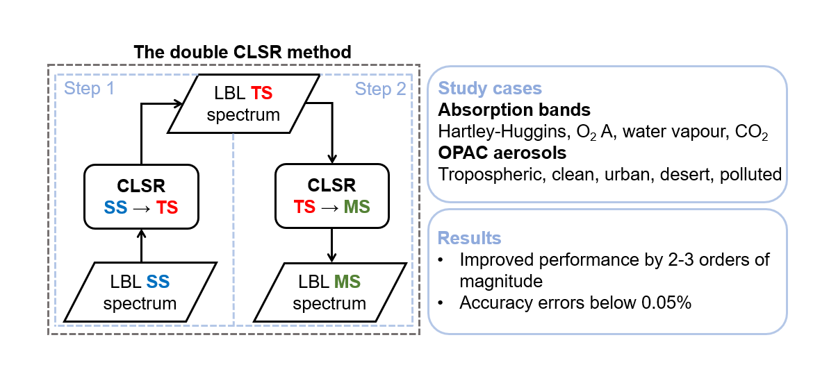
In the double CLSR method, the TS spectra are computed also by applying the CLSR technique. In this case, as an approximate model, we use the single-scattering (SS) RTM. Thus, the algorithm can be described as follows:
Step 1: We compute the LBL spectra by using the SS RTM and apply sorting and clustering to the space of SS radiances. Assuming a regression model between SS and TS radiances within each cluster z, we obtain
with number of radiance points and cluster index z. The regression coefficients are found as a solution of the following least squares problem
where and . By knowing the regression coefficients, the TS spectra can be restored from at high spectral resolution.
Step 2: We apply the CLSR method as described in the previous section (Section 2.2.1) using the TS spectra computed in Step 1.
Figure 2 shows a schematic representation of the CLSR and double CLSR methods. Note that the TS spectra derived at Step 1 by using the CLSR method differ from those computed by the TS RTM in a LBL manner. However, the possible bias obtained in the double CLSR method at Step 1 is removed by the regression model at Step 2.
2.3. CLSR Method: Improvement to Aerosol Scheme
It is important to include aerosols in the simulations, using a numerically efficient RTM to quantify the impact of aerosol scattering [31]. To compute the spectrum in the case of the atmosphere with aerosol, the CLSR and double CLSR methods can be applied. For this case, the regression model (Equation (2)) is used, in which
and the original - matrix is substituted by
where the upper index ’aer’ explicitly says that the computations are performed for the aerosol case. However, as shown in Figure 3, the spectra for the clear sky atmosphere (i.e., Rayleigh atmosphere) with and without aerosols have a similar spectral behaviour, i.e., the aerosol spectra depend almost linearly on the clear sky spectra. In this regard, alternative formulations of the CLSR method can be considered. For instance, taking the - matrix as
we obtain a method, which converts the MS clear sky spectra into spectra corresponding to the aerosol conditions. The upper index ‘clear’ indicates that the computations are performed for the clear sky case. The possible benefit of such a scheme is that the clear sky spectra can be precomputed and stored in LUTs and perform the computations offline, while the computations for actual aerosol properties can be performed online.
Alternatively, we consider the - matrix in the following form:
In this case, the regression model is supplied with the first order perturbation computed by using the TS RTM. As a matter of fact, in this case, we do not expect performance enhancement compared to the -scheme. The question is if the error can be reduced by involving precomputed LUTs for clear sky cases as compared to the original -scheme. Note that for all these cases, the MS RTM for the aerosol scenarios is called for a few spectral points.
3. Results and Discussion
3.1. Single CLSR vs. Double CLSR: Accuracy Results
In this section, we compare the single and double application of the CLSR method in terms of accuracy. To assess it, we compute the relative error (residual) with respect to the continuum at each spectral point in an LBL manner,
where is the radiance calculated with either the CLSR method or the double CLSR method, is the reference radiance with absorption, while is the radiance in the continuum, i.e., without absorption, which is used to avoid values close to zero in the denominator, as in [19]. Other metrics used to estimate the accuracy of the simulations are the mean absolute relative error with respect to the continuum, the probability density functions and the cumulated probability.
Figure 4 shows the probability density function of the spectral residuals for both methods and the four spectral bands. The main conclusions that can be drawn from the figure are the following:
- More than 70% and 60% of the residuals are below 0.01% for the single and double CLSR methods, respectively, for all bands, with the exception of the water vapour band.
- The residuals of the water vapour band present a wider distribution in comparison with the other spectral bands.
- The probability densities are almost indistinguishable for both acceleration methods, demonstrating that both techniques provide accurate results among the different spectral bands.
It can be seen that the accuracy of the CLSR method is slightly higher than that of the double CLSR method. This result can be expected, since the TS spectra used in the double CLSR method are approximate and obtained from the SS spectrum (see Figure 2).
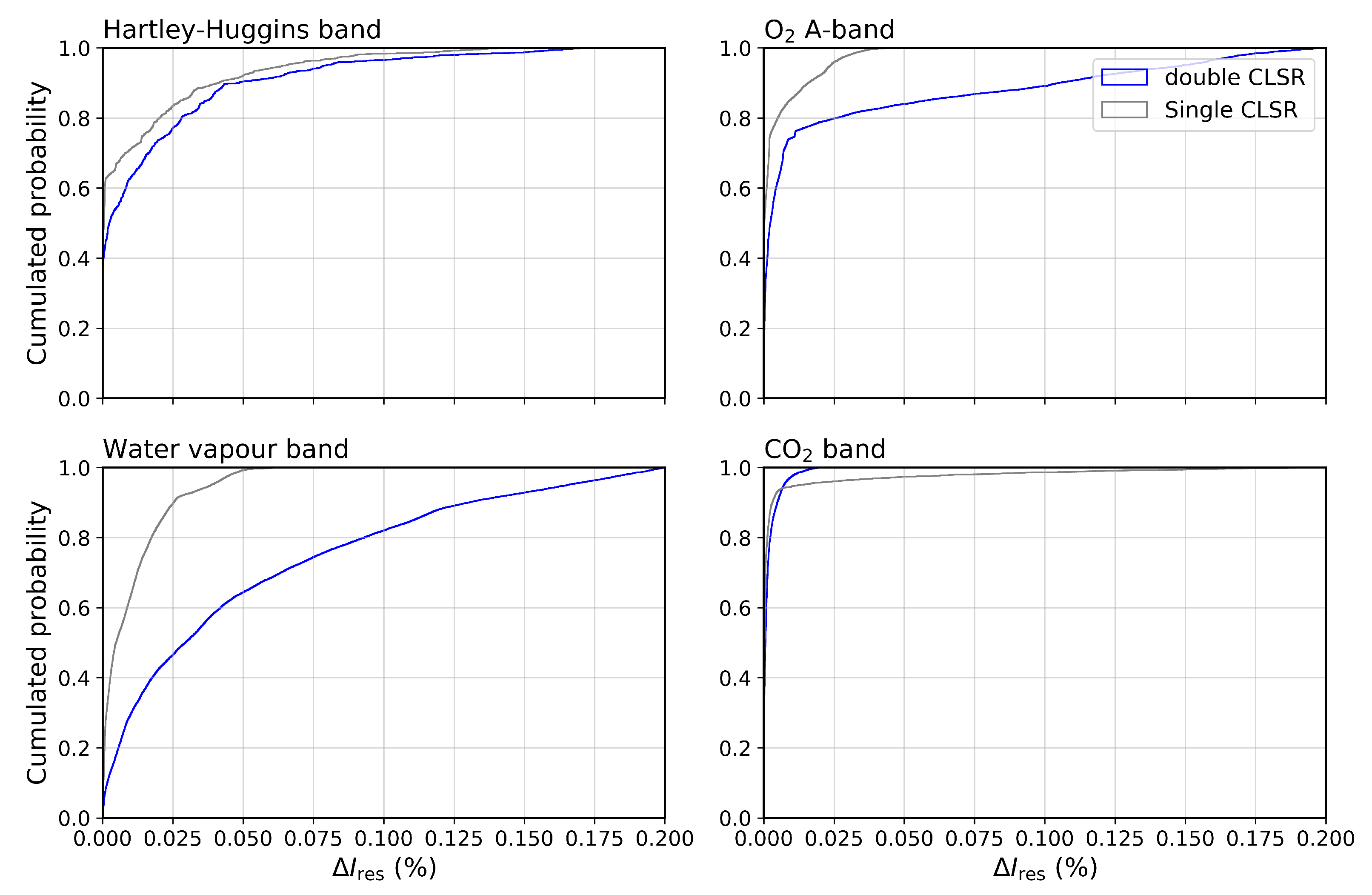
Figure 5 shows the cumulated probability functions of the CLSR and double CLSR methods for all spectral bands. Over 90% residuals are less than 0.05% in the case of the Hartley–Huggins band and 0.01% in the case of the CO band. Higher differences can be seen between the CLSR and double CLSR methods for the OA- and water vapour bands. For these bands, over 90% of the CLSR residuals are less than 0.025%. Meanwhile, the double CLSR provides slightly larger errors: over 60% and 80% of the residuals are less than 0.05% for the O A- and water vapour band, respectively. However, these residual values are still low and of the same order as those obtained by using the PCA-based RTMs. For instance, in Liu et al. [17] PCA was applied to optical parameters and spectral radiances yielding an error lower than 0.2% in the solar region (775–920 nm). Kopparla et al. [19] combined the PCA technique for optical parameters and the spectral binning for accurate computations in the case of aerosols. The residuals were below 0.01% for the O A-band, which are of the same order as our results.
In our previous paper on the CLSR method [14], the convolved spectra were computed, showing errors of the same order as the non-convolved spectra. Here, the same conclusions apply for the double CLSR method.
3.2. Single CLSR vs. Double CLSR: Computational Performance
In this section, we analyse the computational performance of the single and double CLSR methods. Table 2, Table 3 and Table 4 show the number of calls to the SS, TS and MS RTMs, computational times and corresponding acceleration factors with respect to the MS LBL simulations. We recall that, as the reference model, the MS LBL RTM with 32 streams is used.
For the single CLSR method, 5 clusters and 4 regression points per cluster are used. Hence, computations for each absorption band involve 20 MS RTM calls, while the number of TS RTM calls is equal to the number of spectral points in the high-resolution LBL computations (i.e., 300, 20,000 and 40,000 calls to the TS RTM for the Hartley–Huggins, O A- and CO and water vapour band, respectively). As can be seen in Table 2, Table 3 and Table 4, the TS RTM imposes the computational burden of the single CLSR method for the O A-, CO and water vapour bands, consuming up to 70% of the whole computation time.
At the first step of the double CLSR method, 8 clusters and 4 regression points are used. Thus, the TS RTM is called for 32 spectral points. In the case of the double CLSR, the SS RTM is utilized for the LBL computations, resulting in an additional performance enhancement by 2 times for the OA- and CO bands and 3 times for the water vapour band. We note that in the double CLSR, the computational burden corresponds to the MS RTM, while the computation times related to the TS and SS RTMs are three and two orders of magnitude lower than those of the MS RTM, respectively. In the case of the Hartley–Huggins band, the computational burden is still due to the MS RTM [12] and the double CLSR does not further improve the performance.
As a final remark, the accuracy is crucial to determine the number of calls needed for the CLSR methods, and we could improve it by increasing the number of calls to the RTM models. However, this would add a computational burden to the simulations, while providing little improvement in the accuracy. Several tests have been performed by increasing the number of calls to the SS RTM or TS RTM but the errors are of the same order of magnitude as the actual values.
3.3. Computational Performance: State-of-the-Art Acceleration Techniques
In this section, we compare the CLSR and double CLSR methods against other state-of-the-art acceleration techniques. Table 5 summarizes the spectral bands/regions and the acceleration factors for the selected acceleration techniques, including this study. In this analysis, we consider the studies covering absorption bands in the 280–3000 nm spectral range.
Note that the acceleration factors depend not only on the method used, but also on other aspects, such as the number of discrete ordinates used for the reference RTM. In turn, the required number of depends on aerosol properties, surface properties, geometry and the required accuracy. Therefore, the acceleration factors are ambiguous, as different numbers of streams or atmospheric parameters are used for the reference RTM in the different studies. Nevertheless, the following conclusions can be made:
- For simulations in the Hartley–Huggins band, PCA techniques, linear embedding methods (LEM) and double CLSR have been applied. The double CLSR does not further improve the performance, since the computational burden is due to the MS RTM computations (see Section 3.2). The highest acceleration factor is provided by the method described in [12], in which PCA is applied to both optical parameters and spectral radiances. The performance enhancement in this case is up to 18 times.
- There are several studies in which fast RTMs for the O A- and CO bands (either weak or strong) have been designed. In general, all considered techniques provide acceleration factors of about 2–3 orders of magnitude, including those based on artificial neural networks (NN) [37].
- The water vapour band represents a challenge for acceleration techniques due to its complicated spectral structure. Therefore, the accuracy of the acceleration techniques is lower than for the O A-band. For this band, the double CLSR method provides an acceleration factor of about 3 orders of magnitude, while the k-distribution [32] and PCA-based RTMs [19] achieve lower acceleration factors, of one order of magnitude.
3.4. Further Improvements to Aerosol Schemes
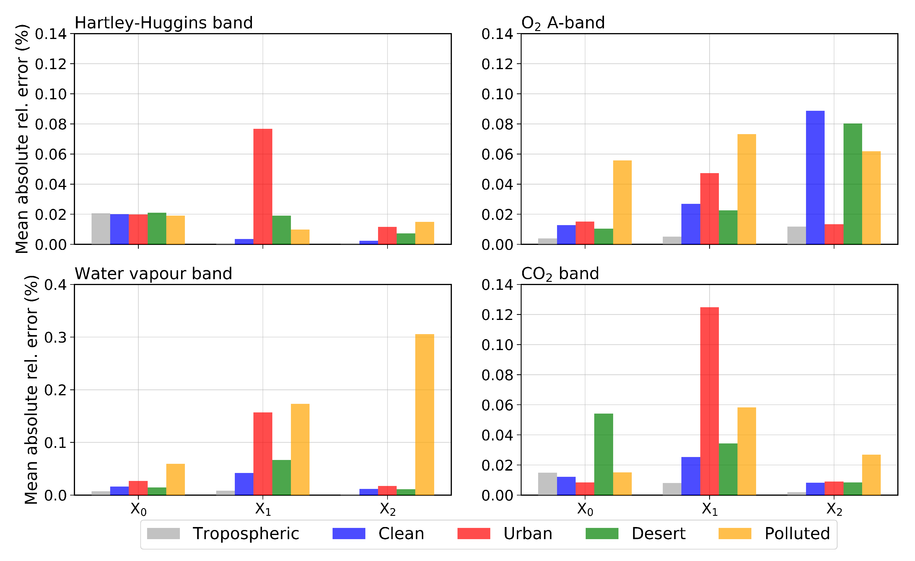
In this section, the efficiency of the CLSR method for various configurations outlined in Section 2.3 is examined for several OPAC aerosol models. The results obtained using and (corresponding to Equations (9) and (10), respectively) are compared against the original CLSR method in which the matrix (Equation (8)) is used. The mean absolute relative errors are shown in Figure 6. In general, mean relative absolute errors are below 0.05% for all aerosol types and bands when using the original -configuration for the CLSR method. However, these errors are slightly higher for the water vapour band due to its higher spectral complexity.
Almost in all cases, the configuration is less accurate than the original CLSR method. This result can be expected, as carries no information about the radiances of aerosols. However, for low aerosol load (tropospheric and clean aerosols), the errors are of the same order or below 0.05% compared to the ones from . The advantage of the configuration is that it is based on spectra computed for the clear sky atmosphere. The corresponding LUT, therefore, is independent on aerosol properties. By using the CLSR method, the spectrum for actual aerosol conditions can be computed by calling MS RTM at a few spectral points (in our case, 20 spectral points).
The configuration comprises , which contains the spectra corresponding to the TS RTM, and , which corresponds to TS and MS RTMs for clear sky scenarios. An improvement with respect to the original configuration is provided by the -configuration for the Hartley–Huggins and CO bands, where absolute relative errors are of the same order as for -configuration or below 0.01%. For the O A-band, there is almost no enhancement compared to the original configuration. We have excluded the transmittance in the numerical simulations for the CO band in order to obtain slightly more accurate results.
In sum, we present two alternative configurations to the original , in order to obtain more accurate results for: (1) low aerosol loading conditions with the configuration for all bands; and (2) the Hartley–Huggins, water vapour and CO bands with the configuration.
3.5. Combined Application of the Single CLSR vs. Double CLSR Method for Aerosol Scenarios
Finally, the single and double CLSR methods are tested for the full set of aerosol models and -configurations. The probability density functions of the residuals for the tropospheric aerosol model are shown in Figure 7 and Figure 8.
The conclusions drawn from the comparison of the two figures can be summarized as follows:
- The residual distributions of the single CLSR method are narrower than those of the double CLSR method, meaning that the single CLSR method is more accurate. However, in general, the residuals are below 0.01% for both methods and all spectral bands, except for the water vapour band, where the residual distributions are slightly wider and still below 0.05%. The distributions are not biased.
- For the Hartley–Huggins, O A- and CO bands, the residuals are below 0.05% for both single and double CLSR methods. Regarding the water vapour band, the residuals are below 0.05% and 0.1% for the single and double CLSR method, respectively. Similar accuracies were achieved in Kopparla et al. [19] for the water vapour band using the PCA-based RTM.
- In the case of the low aerosol load, the probability density functions are similar for all -configurations. However, as the aerosol load increases, the residual distributions for the configuration provided by the single and double CLSR methods sometimes become biased for the water vapour band.
4. Conclusions
In this study, we have proposed two modifications to the CLSR method for fast computations of radiance spectra in absorption bands. In the first modification, the CLSR method is used twice, the first time for assessing the spectra corresponding to the TS RTM, and the second time for computing the spectra corresponding to the MS RTM. Our tests reveal that the double CLSR method further improves the computational performance of the original CLSR method by two (CO and OA- bands) and three times (water vapour band), yet keeping the error below 0.05% for all spectral points on a high resolution grid. The designed approach has been compared with the state-of-the-art techniques found in the literature. Although the acceleration factors are ambiguous, in our simulations, the double CLSR method seems to provide a slightly higher performance than the PCA-based RTMs.
The second modification of the CLSR method is proposed for the atmospheric scenarios involving aerosols. The LBL computations performed for clear sky scenarios can be reused in the CLSR method as an approximate spectrum instead of the TS RTM, which is then corrected by calling the RTM for the atmospheric model with aerosol, but in a few spectral points. Therefore, by using the configuration of the CLSR method only with the information of the clear sky spectra, we can reproduce the LBL spectra with low aerosol load. We showed that in the case of low aerosol load, such a configuration provides absolute relative errors below 0.05% for all spectral bands, while enhancing the computational performance by three orders of magnitude. Low aerosol loading conditions occur when the atmosphere is in practice mainly clean. As the aerosol load increases (e.g., for polluted aerosol, with AOD equal to 5), the error also increases and reaches ∼0.2% for water vapour band and ∼0.1% in the O A- and CO band. The new configurations have been tested for both CLSR and double CLSR methods, revealing similar probability density functions. These results have the potential to be applied in near-real-time applications of aerosol computations or in aerosol retrieval algorithms considering an appropriate aerosol model selection [38,39]. It also seems beneficial to implement the CLSR method in conjunction with gradient-based LUT generators [40,41], to reduce the size of LUTs and interpolation errors. Besides, the CLSR method provides an accurate alternative to the LUT interpolation, which combines the regression and online RTM simulations. Therefore, the single and double CLSR methods could potentially be incorporated into the generation of LUT radiance fields in a fine resolution grid.
Our future work will be focused on coupling the CLSR method and machine learning approaches. Recent studies have shown that the accuracy of hyperspectral radiative transfer simulations can be improved by applying machine learning techniques (e.g., see [37]). Essentially, NNs are used as universal approximators which replace time-consuming RTMs. Further studies will be undertaken to replace the regression model with an NN, within the framework of the CLSR method. By doing this, we expect to reduce the number of clusters and spectral points for which the MS RTM is called.
Author Contributions
Conceptualization, A.d.Á.; methodology, A.d.Á.; software, A.d.Á.; formal analysis, D.S.E.; investigation, A.d.Á.; writing—original draft preparation, A.d.Á.; writing—review and editing, D.S.E.; visualization, A.d.Á.; supervision, D.S.E.; funding acquisition, D.S.E. All authors have read and agreed to the published version of the manuscript.
Funding
Institutional Review Board Statement
Not applicable.
Informed Consent Statement
Not applicable.
Data Availability Statement
Not applicable.
Conflicts of Interest
The authors declare no conflict of interest.
Abbreviations
The following abbreviations are used in this manuscript:
| AOD | Aerosol Optical Depth |
| CLSR | Cluster Low-Streams Interpolation |
| DOME | Discrete Ordinates with Matrix Exponential |
| HITRAN | High-Resolution Transmission Molecular Absorption Database |
| LBL | Line-By-Line |
| LEM | Linear Embedding Methods |
| LSI | Low-Streams Interpolation |
| LUT | LookUp Table |
| MS | Multi-Stream |
| NN | Neural Network |
| OPAC | Optical Properties of Aerosols and Clouds |
| PCA | Principal Component Analysis |
| Py4CAts | Python for Computational Atmospheric Spectroscopy |
| RTM | Radiative Transfer Model |
| SDCOMP | Spectral Data Compression |
| SS | Single-Scattering |
| SSA | Single Scattering Albedo |
| TOA | Top-of-the-Atmosphere |
| TS | Two-Stream |
| UV | Ultraviolet |
References
- Goody, R.; West, R.; Chen, L.; Crisp, D. The correlated-k method for radiation calculations in nonhomogeneous atmospheres. J. Quant. Spectrosc. Radiat. Transf. 1989, 42, 539–550. [Google Scholar] [CrossRef]
- Fu, Q.; Liou, K. On the correlated k-distribution method for radiative transfer in nonhomogeneous atmospheres. J. Atmos. Sci. 1992, 49, 2139–2156. [Google Scholar] [CrossRef] [Green Version]
- Kato, S.; Ackerman, T.P.; Mather, J.H.; Clothiaux, E.E. The k-distribution method and correlated-k approximation for a shortwave radiative transfer model. J. Quant. Spectrosc. Radiat. Transf. 1999, 62, 109–121. [Google Scholar] [CrossRef]
- Zhang, F.; Zhu, M.; Li, J.; Li, W.; Di, D.; Shi, Y.N.; Wu, K. Alternate Mapping Correlated k-Distribution Method for Infrared Radiative Transfer Forward Simulation. Remote Sens. 2019, 11, 994. [Google Scholar] [CrossRef] [Green Version]
- O’Dell, C.W. Acceleration of multiple-scattering, hyperspectral radiative transfer calculations via low-streams interpolation. J. Geophys. Res. 2010, 115. [Google Scholar] [CrossRef]
- Natraj, V.; Jiang, X.; Shia, R.; Huang, X.; Margolis, J.; Yung, Y. Application of the principal component analysis to high spectral resolution radiative transfer: A case study of the O2 A-band. J. Quant. Spectrosc. Radiat. Transf. 2005, 95, 539–556. [Google Scholar] [CrossRef]
- Kopparla, P.; Natraj, V.; Spurr, R.; Shia, R.L.; Crisp, D.; Yung, Y.L. A fast and accurate PCA based radiative transfer model: Extension to the broadband shortwave region. J. Quant. Spectrosc. Radiat. Transf. 2016, 173, 65–71. [Google Scholar] [CrossRef]
- Efremenko, D.; Doicu, A.; Loyola, D.; Trautmann, T. Acceleration techniques for the discrete ordinate method. J. Quant. Spectrosc. Radiat. Transf. 2013, 114, 73–81. [Google Scholar] [CrossRef]
- Efremenko, D.; Doicu, A.; Loyola, D.; Trautmann, T. Optical property dimensionality reduction techniques for accelerated radiative transfer performance: Application to remote sensing total ozone retrievals. J. Quant. Spectrosc. Radiat. Transf. 2014, 133, 128–135. [Google Scholar] [CrossRef]
- Liu, X.; Smith, W.L.; Zhou, D.K.; Larar, A. Principal component-based radiative transfer model for hyperspectral sensors: Theoretical concept. Appl. Opt. 2006, 45, 201–208. [Google Scholar] [CrossRef]
- Molina García, V.; Sasi, S.; Efremenko, D.; Doicu, A.; Loyola, D. Radiative transfer models for retrieval of cloud parameters from EPIC/DSCOVR measurements. J. Quant. Spectrosc. Radiat. Transf. 2018, 213, 228–240. [Google Scholar] [CrossRef] [Green Version]
- del Águila, A.; Efremenko, D.S.; Molina García, V.; Xu, J. Analysis of two dimensionality reduction techniques for fast simulation of the spectral radiances in the Hartley-Huggins band. Atmosphere 2019, 10, 142. [Google Scholar] [CrossRef] [Green Version]
- del Águila, A.; Efremenko, D.S.; Trautmann, T. A review of dimensionality reduction techniques for processing hyper-spectral optical signal. Light Eng. 2019, 27, 85–98. [Google Scholar] [CrossRef] [Green Version]
- del Águila, A.; Efremenko, D.S.; Molina García, V.; Kataev, M.Y. Cluster Low-Streams Regression Method for Hyperspectral Radiative Transfer Computations: Cases of O2 A- and CO2 Bands. Remote Sens. 2020, 12, 1250. [Google Scholar] [CrossRef] [Green Version]
- Vincent, R.A.; Dudhia, A. Fast radiative transfer using monochromatic look-up tables. J. Quant. Spectrosc. Radiat. Transf. 2017, 186, 254–264. [Google Scholar] [CrossRef] [Green Version]
- Duan, M.; Min, Q.; Li, J. A fast radiative transfer model for simulating high-resolution absorption bands. J. Geophys. Res. Atmos. 2005, 110. [Google Scholar] [CrossRef] [Green Version]
- Liu, C.; Yao, B.; Natraj, V.; Kopparla, P.; Weng, F.; Le, T.; Shia, R.L.; Yung, Y.L. A Spectral Data Compression (SDCOMP) Radiative Transfer Model for High-Spectral-Resolution Radiation Simulations. J. Atmos. Sci. 2020, 77, 2055–2066. [Google Scholar] [CrossRef] [Green Version]
- Doicu, A.; Efremenko, D.; Trautmann, T. A Spectral Acceleration Approach for the Spherical Harmonics Discrete Ordinate Method. Remote Sens. 2020, 12, 3703. [Google Scholar] [CrossRef]
- Kopparla, P.; Natraj, V.; Limpasuvan, D.; Spurr, R.; Crisp, D.; Shia, R.L.; Somkuti, P.; Yung, Y.L. PCA-based radiative transfer: Improvements to aerosol scheme, vertical layering and spectral binning. J. Quant. Spectrosc. Radiat. Transf. 2017, 198, 104–111. [Google Scholar] [CrossRef]
- Schreier, F.; Gimeno García, S.; Hochstaffl, P.; Städt, S. Py4CAtS—PYthon for Computational Atmospheric Spectroscopy. Atmosphere 2019, 10, 262. [Google Scholar] [CrossRef] [Green Version]
- Gordon, I.; Rothman, L.; Hill, C.; Kochanov, R.; Tan, Y.; Bernath, P.; Birk, M.; Boudon, V.; Campargue, A.; Chance, K.; et al. The HITRAN2016 molecular spectroscopic database. J. Quant. Spectrosc. Radiat. Transf. 2017, 203, 3–69. [Google Scholar] [CrossRef]
- Bodhaine, B.; Wood, N.; Dutton, E.; Slusser, J. On Rayleigh optical depth calculations. J. Atmos. Ocean. Technol. 1999, 16, 1854–1861. [Google Scholar] [CrossRef]
- Anderson, G.; Clough, S.; Kneizys, F.; Chetwynd, J.; Shettle, E. AFGL Atmospheric Constituent Profiles (0.120 km); Air ForceGeophysics Lab.: Hanscom AFB, MA, USA, 1986; p. 46. [Google Scholar]
- Doicu, A.; Trautmann, T. Discrete-ordinate method with matrix exponential for a pseudo-spherical atmosphere: Scalar case. J. Quant. Spectrosc. Radiat. Transf. 2009, 110, 146–158. [Google Scholar] [CrossRef]
- Efremenko, D.S.; Molina García, V.; Gimeno García, S.; Doicu, A. A review of the matrix-exponential formalism in radiative transfer. J. Quant. Spectrosc. Radiat. Transf. 2017, 196, 17–45. [Google Scholar] [CrossRef] [Green Version]
- Wiscombe, W.J. The Delta-M Method: Rapid Yet Accurate Radiative Flux Calculations for Strongly Asymmetric Phase Functions. J. Atmos. Sci. 1977, 34, 1408–1422. [Google Scholar] [CrossRef] [Green Version]
- Nakajima, T.; Tanaka, M. Algorithms for radiative intensity calculations in moderately thick atmospheres using a truncation approximation. J. Quant. Spectrosc. Radiat. Transf. 1988, 40, 51–69. [Google Scholar] [CrossRef]
- Fischer, J.; Grassl, H. Radiative transfer in an atmosphere-ocean system: An azimuthally dependent matrix-operator approach. Appl. Opt. 1984, 23, 1032. [Google Scholar] [CrossRef]
- Chalhoub, E.; Garcia, R. The equivalence between two techniques of angular interpolation for the discrete-ordinates method. J. Quant. Spectrosc. Radiat. Transf. 2000, 64, 517–535. [Google Scholar] [CrossRef]
- Hess, M.; Koepke, P.; Schult, I. Optical properties of aerosols and clouds: The software package OPAC. Bull. Am. Meteorol. Soc. 1998, 79, 831–844. [Google Scholar] [CrossRef]
- Huang, Y.; Natraj, V.; Zeng, Z.C.; Kopparla, P.; Yung, Y.L. Quantifying the impact of aerosol scattering on the retrieval of methane from airborne remote sensing measurements. Atmos. Meas. Tech. 2020, 13, 6755–6769. [Google Scholar] [CrossRef]
- Fomin, B. A k-distribution technique for radiative transfer simulation in inhomogeneous atmosphere: 2. FKDM, fast k-distribution model for the shortwave. J. Geophys. Res. 2005, 110. [Google Scholar] [CrossRef] [Green Version]
- Natraj, V.; Shia, R.L.; Yung, Y.L. On the use of principal component analysis to speed up radiative transfer calculations. J. Quant. Spectrosc. Radiat. Transf. 2010, 111, 810–816. [Google Scholar] [CrossRef]
- Spurr, R.; Natraj, V.; Lerot, C.; Roozendael, M.V.; Loyola, D. Linearization of the Principal Component Analysis method for radiative transfer acceleration: Application to retrieval algorithms and sensitivity studies. J. Quant. Spectrosc. Radiat. Transf. 2013, 125, 1–17. [Google Scholar] [CrossRef]
- Efremenko, D.S.; Loyola, D.G.; Spurr, R.J.; Doicu, A. Acceleration of radiative transfer model calculations for the retrieval of trace gases under cloudy conditions. J. Quant. Spectrosc. Radiat. Transf. 2014, 135, 58–65. [Google Scholar] [CrossRef]
- Somkuti, P.; Boesch, H.; Natraj, V.; Kopparla, P. Application of a PCA-Based Fast Radiative Transfer Model to XCO2 Retrievals in the Shortwave Infrared. J. Geophys. Res. Atmos. 2017, 122, 10,477–10,496. [Google Scholar] [CrossRef]
- Le, T.; Liu, C.; Yao, B.; Natraj, V.; Yung, Y.L. Application of machine learning to hyperspectral radiative transfer simulations. J. Quant. Spectrosc. Radiat. Transf. 2020, 246, 106928. [Google Scholar] [CrossRef]
- Sasi, S.; Natraj, V.; Molina García, V.; Efremenko, D.; Loyola, D.; Doicu, A. Model Selection in Atmospheric Remote Sensing with an Application to Aerosol Retrieval from DSCOVR/EPIC, Part 1: Theory. Remote Sens. 2020, 12, 3724. [Google Scholar] [CrossRef]
- Sasi, S.; Natraj, V.; Molina García, V.; Efremenko, D.; Loyola, D.; Doicu, A. Model Selection in Atmospheric Remote Sensing with Application to Aerosol Retrieval from DSCOVR/EPIC. Part 2: Numerical Analysis. Remote Sens. 2020, 12, 3656. [Google Scholar] [CrossRef]
- Vicent, J.; Verrelst, J.; Rivera-Caicedo, J.P.; Sabater, N.; Muñoz-Marí, J.; Camps-Valls, G.; Moreno, J. Emulation as an Accurate Alternative to Interpolation in Sampling Radiative Transfer Codes. IEEE J. Sel. Top. Appl. Earth Obs. Remote Sens. 2018, 11, 4918–4931. [Google Scholar] [CrossRef]
- Vicent Servera, J.; Alonso, L.; Martino, L.; Sabater, N.; Verrelst, J.; Camps-Valls, G.; Moreno, J. Gradient-Based Automatic Lookup Table Generator for Radiative Transfer Models. IEEE Trans. Geosci. Remote Sens. 2019, 57, 1040–1048. [Google Scholar] [CrossRef]
Figure 1.
Overview of the optical properties (AOD, SSA and g) obtained from the OPAC database for the aerosol types: tropospheric, clean continental, urban, desert and polluted. Each vertical line corresponds with the middle wavelength of the spectral bands in order: Hartley–Huggins, O A, water vapour and CO bands.

Figure 2.
Scheme of the CLSR method vs. the double CLSR method.

Figure 3.
TOA radiances computed by using the MS RTM for the absorption bands: Hartley–Huggins, O A-, water vapour and CO bands. Blue lines correspond to the case without aerosol, while the black lines correspond to the specific case of desert aerosol.
Figure 3.
TOA radiances computed by using the MS RTM for the absorption bands: Hartley–Huggins, O A-, water vapour and CO bands. Blue lines correspond to the case without aerosol, while the black lines correspond to the specific case of desert aerosol.

Figure 4.
Probability density function of the residuals for the single CLSR (grey) and the double CLSR (blue) methods for the Hartley–Huggins, O A-, water vapour and CO bands and for the tropospheric aerosol case.
Figure 4.
Probability density function of the residuals for the single CLSR (grey) and the double CLSR (blue) methods for the Hartley–Huggins, O A-, water vapour and CO bands and for the tropospheric aerosol case.

Figure 5.
Same as Figure 4, but for the cumulated probability of the residuals.
Figure 5.
Same as Figure 4, but for the cumulated probability of the residuals.

Figure 6.
Mean absolute relative error in % for the four spectral bands, as well as for all aerosol types. Each bar colour corresponds to an aerosol type, while each group of bars corresponds to one of the -matrix () (Equations (8)–(10)) used in the CLSR method. Note that the scale of the water vapour band is different from the rest of the spectral bands.

Figure 7.
Probability density of the residuals for the single CLSR method and for several matrix configurations: , and . Each plot represents the absorption bands: Hartley–Huggins, O A-, water vapour and CO bands. The case presented corresponds to the tropospheric aerosol.
Figure 7.
Probability density of the residuals for the single CLSR method and for several matrix configurations: , and . Each plot represents the absorption bands: Hartley–Huggins, O A-, water vapour and CO bands. The case presented corresponds to the tropospheric aerosol.

Figure 8.
Same as Figure 7, but for the double CLSR method.
Figure 8.
Same as Figure 7, but for the double CLSR method.


Table 1.
Spectral ranges, resolutions and number of spectral points for the absorption bands used in this study.
Table 1.
Spectral ranges, resolutions and number of spectral points for the absorption bands used in this study.
| Band | Spectral Range (nm) | Spectral Resolution (nm) | Number of Spectral Points |
|---|---|---|---|
| Hartley–Huggins | 280–335 | 0.18 | 300 |
| O A | 755–775 | 0.0010 | 20,000 |
| Water vapour | 770–1000 | 0.0058 | 40,000 |
| CO | 1590–1620 | 0.0015 | 20,000 |
Table 2.
Summary of number of calls, computational time and acceleration factors for the Hartley–Huggins band. The computational times marked in red indicate the computational burden.
Table 2.
Summary of number of calls, computational time and acceleration factors for the Hartley–Huggins band. The computational times marked in red indicate the computational burden.
| RTM | LBL | Single CLSR | Double CLSR | |
|---|---|---|---|---|
| Number of calls | MS | 300 | 20 | 20 |
| TS | 0 | 300 | 32 | |
| SS | 0 | 0 | 300 | |
| Computation time (s) | MS | 35 | 2.32 | 2.32 |
| TS | 0 | 0.048 | 0.005 | |
| SS | 0 | 0 | 0.006 | |
| Total computational time (s) | 35 | 2.37 | 2.33 | |
| Acceleration factor | – | 14.8 | 15.0 |
Table 3.
Same as for Table 2 but for the OA- and CO bands.
Table 3.
Same as for Table 2 but for the OA- and CO bands.
| RTM | LBL | Single CLSR | Double CLSR | |
|---|---|---|---|---|
| Number of calls | MS | 20,000 | 20 | 20 |
| TS | 0 | 20,000 | 32 | |
| SS | 0 | 0 | 20,000 | |
| Computation time (s) | MS | 2320 | 2.32 | 2.32 |
| TS | 0 | 3.2 | 0.005 | |
| SS | 0 | 0 | 0.4 | |
| Total computational time (s) | 2320 | 5.52 | 2.725 | |
| Acceleration factor | – | 420 | 850 |
Table 4.
Same as for Table 2 but for the water vapour band.
Table 4.
Same as for Table 2 but for the water vapour band.
| RTM | LBL | Single CLSR | Double CLSR | |
|---|---|---|---|---|
| Number of calls | MS | 40,000 | 20 | 20 |
| TS | 0 | 40,000 | 32 | |
| SS | 0 | 0 | 40,000 | |
| Computation time (s) | MS | 4640 | 2.32 | 2.32 |
| TS | 0 | 6.4 | 0.005 | |
| SS | 0 | 0 | 0.8 | |
| Total computational time (s) | 4640 | 8.72 | 3.13 | |
| Acceleration factor | – | 532 | 1482 |
Table 5.
Selected acceleration techniques with the corresponding spectral region or band, acceleration factor (computed with respect to the LBL model) and their reference. Note that the acceleration factors are sometimes given in orders of magnitude compared to the LBL approach. One or two order of magnitude are indicated as 10× and 100×, respectively. The references are ordered chronologically.
| Acceleration Technique | Band/Spectral Region | Acceleration Factor | Reference |
|---|---|---|---|
| k-distribution | HO, CO, O, and O | 10× * | Fomin [32] |
| double-k approach | O A | 1000 | Duan [16] |
| LSI | O A, CO weak, CO strong | 45 , 210 | O’Dell [5] |
| PCA | O A, CO weak, CO strong | 50 | Natraj et al. [33] |
| PCA | 290–340 nm | 10 | Spurr et al. [34] |
| LEM | 325–335 nm | 10 | Efremenko et al. [9] |
| PCA | 325–335 nm | 2 | Efremenko et al. [35] |
| PCA | 300–3000 nm | 10× | Kopparla et al. [19] |
| PCA | O A, CO weak, CO strong | 100× | Somkuti et al. [36] |
| k-distribution + PCA | O A | 342 | Molina García et al. [11] |
| PCA | Hartley-Huggins | 18 | del Águila et al. [12] |
| NN | O A, CO weak, CO strong | 250 | Le et al. [37] |
| LEM | NO (425–450 nm) | 12 e | Doicu et al. [18] |
| CLSR | O A, CO weak | 505 | del Águila et al. [14] |
| SDCOMP | 750–920 nm | 1000 | Liu et al. [17] |
| double CLSR | Hartley-Huggins | 15 | This study |
| O A, CO weak | 850 | ||
| Water vapour | 1500 |
PCA is applied twice, (1) to the optical properties and (2) the radiance data set. Nadir observations. Glint observations. Computation times are not considered, only the relative computational efficiency with respect to the accurate simulations. e Relative to the k-distribution method. * It is estimated from the information found in the reference, but the value does not appear explicitly.
Publisher’s Note: MDPI stays neutral with regard to jurisdictional claims in published maps and institutional affiliations. |
© 2021 by the authors. Licensee MDPI, Basel, Switzerland. This article is an open access article distributed under the terms and conditions of the Creative Commons Attribution (CC BY) license (http://creativecommons.org/licenses/by/4.0/).
Share and Cite
MDPI and ACS Style
del Águila, A.; Efremenko, D.S. Fast Hyper-Spectral Radiative Transfer Model Based on the Double Cluster Low-Streams Regression Method. Remote Sens. 2021, 13, 434. https://0-doi-org.brum.beds.ac.uk/10.3390/rs13030434
AMA Style
del Águila A, Efremenko DS. Fast Hyper-Spectral Radiative Transfer Model Based on the Double Cluster Low-Streams Regression Method. Remote Sensing. 2021; 13(3):434. https://0-doi-org.brum.beds.ac.uk/10.3390/rs13030434
Chicago/Turabian Styledel Águila, Ana, and Dmitry S. Efremenko. 2021. "Fast Hyper-Spectral Radiative Transfer Model Based on the Double Cluster Low-Streams Regression Method" Remote Sensing 13, no. 3: 434. https://0-doi-org.brum.beds.ac.uk/10.3390/rs13030434
Note that from the first issue of 2016, this journal uses article numbers instead of page numbers. See further details here.