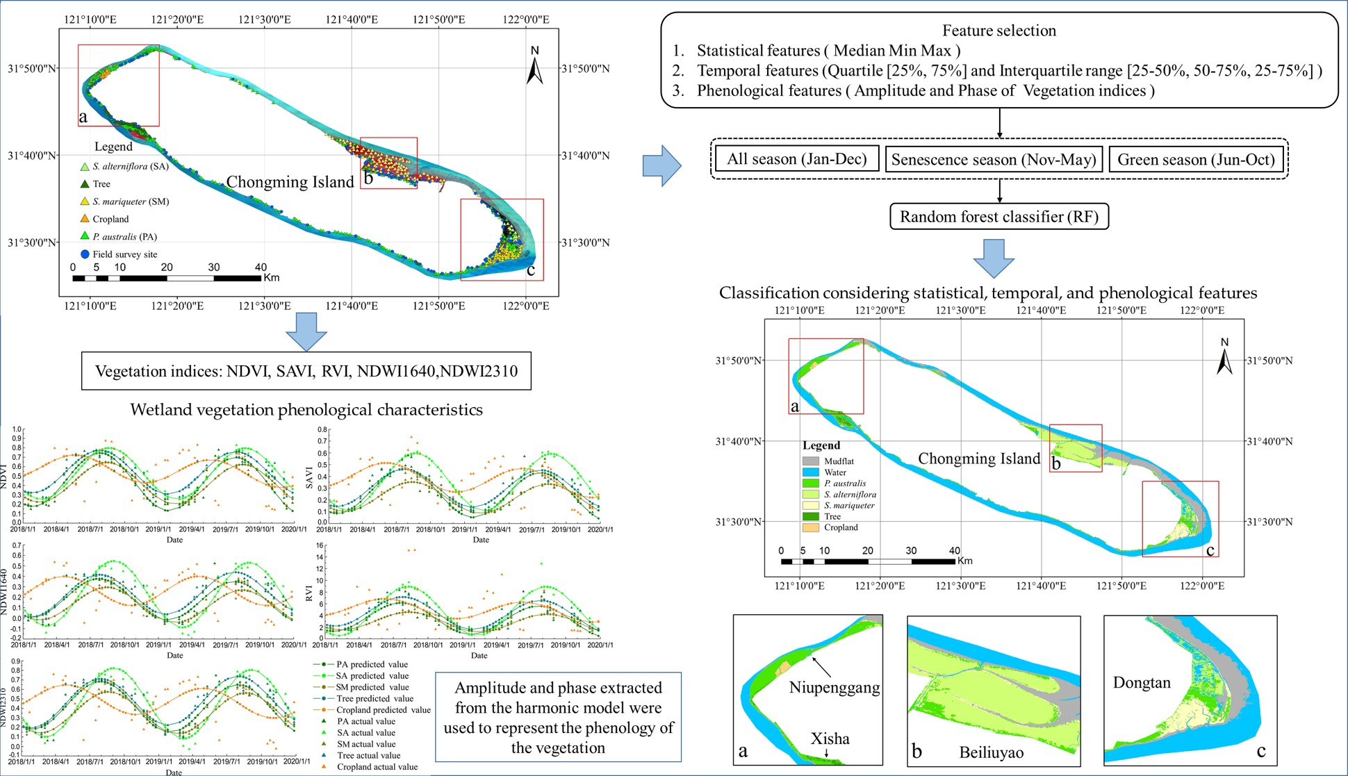
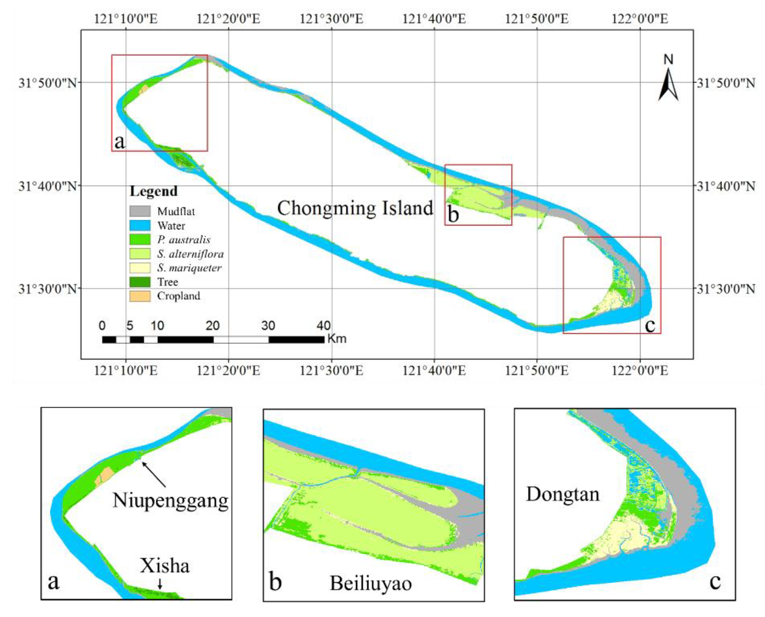
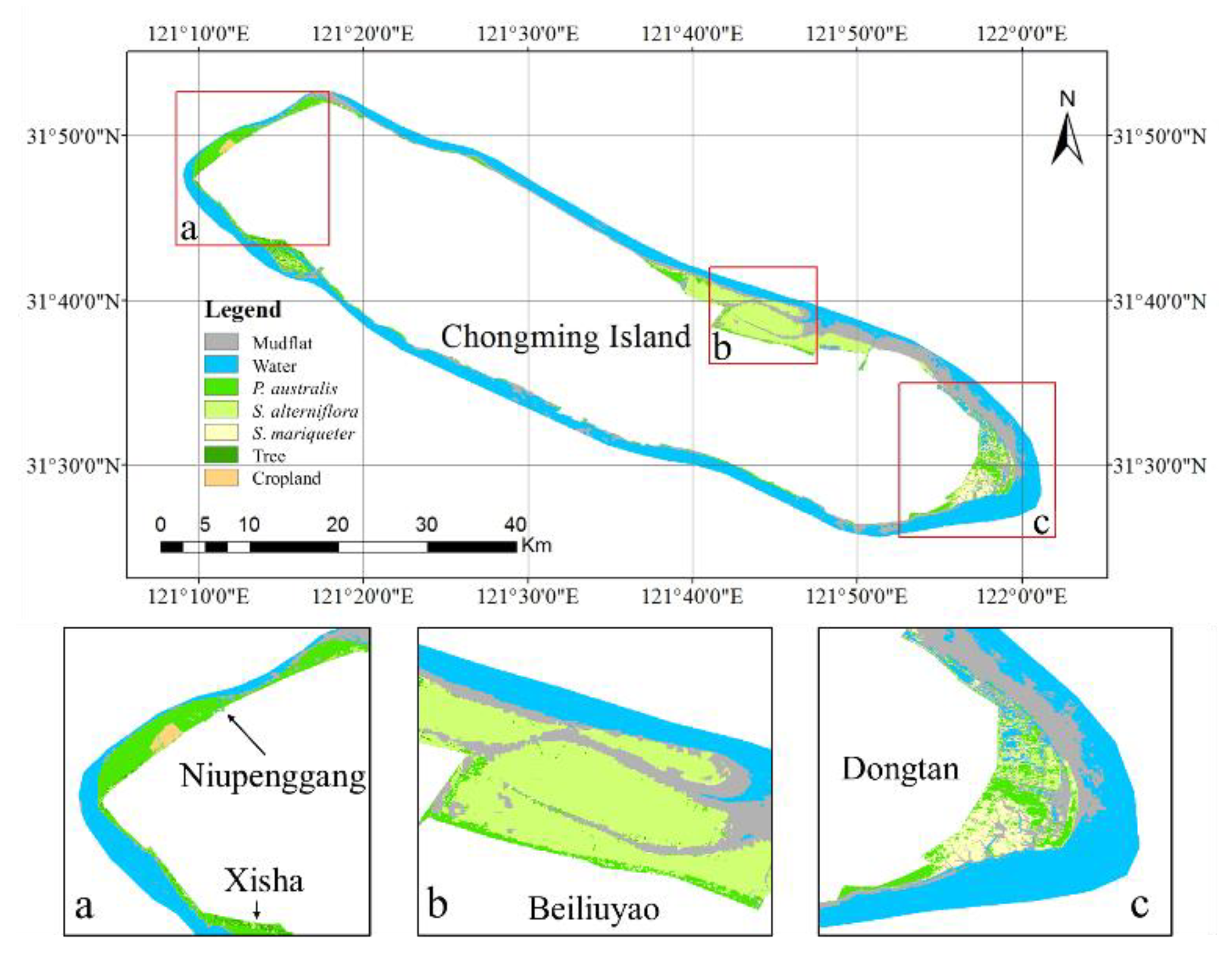
Figure 1.
Distribution of the study area. The base map in
Figure 1 is from a Landsat 8 Operational Land Imager (OLI) image obtained on 17 December 2018, and displayed in false color with near-infrared, red, and green bands. The subfigures are zoomed-in images and prominently show the main distribution area of the tidal flat wetland vegetation of Chongming Island. Subfigure (
a) shows the Xisha and Niupenggang areas, subfigure (
b) shows the Beiliuyao area, and subfigure (
c) shows the Dongtan area. The triangular points in the legend represent the sample points of various types of vegetation selected in the study, and the blue circular points represent the locations of the field survey sites.
Figure 2.
Experimental flowchart.
Figure 2.
Experimental flowchart.
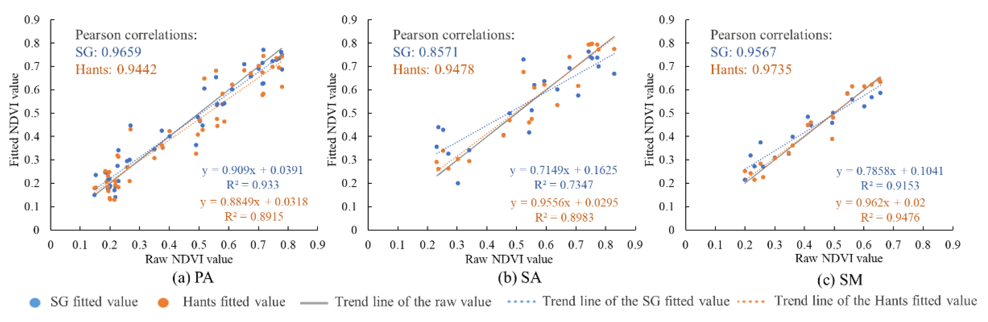
Figure 3.
Comparison of the fitting effects of the Hants and Savitzky–Golay (SG) filtering methods for the mean normalized difference vegetation index (NDVI) of (a) P. australis, (b) S. alterniflora and (c) S. mariqueter.
Figure 3.
Comparison of the fitting effects of the Hants and Savitzky–Golay (SG) filtering methods for the mean normalized difference vegetation index (NDVI) of (a) P. australis, (b) S. alterniflora and (c) S. mariqueter.
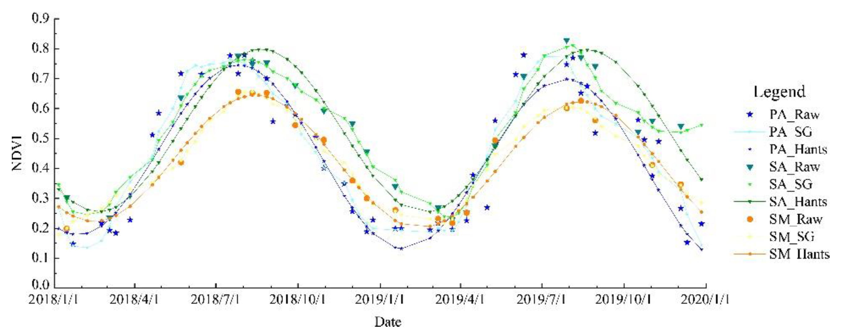
Figure 4.
Comparison of Hants and SG filtering methods used to extract wetland vegetation phenology based on the average NDVI value across each vegetation type at the time of each Landsat image.
Figure 4.
Comparison of Hants and SG filtering methods used to extract wetland vegetation phenology based on the average NDVI value across each vegetation type at the time of each Landsat image.
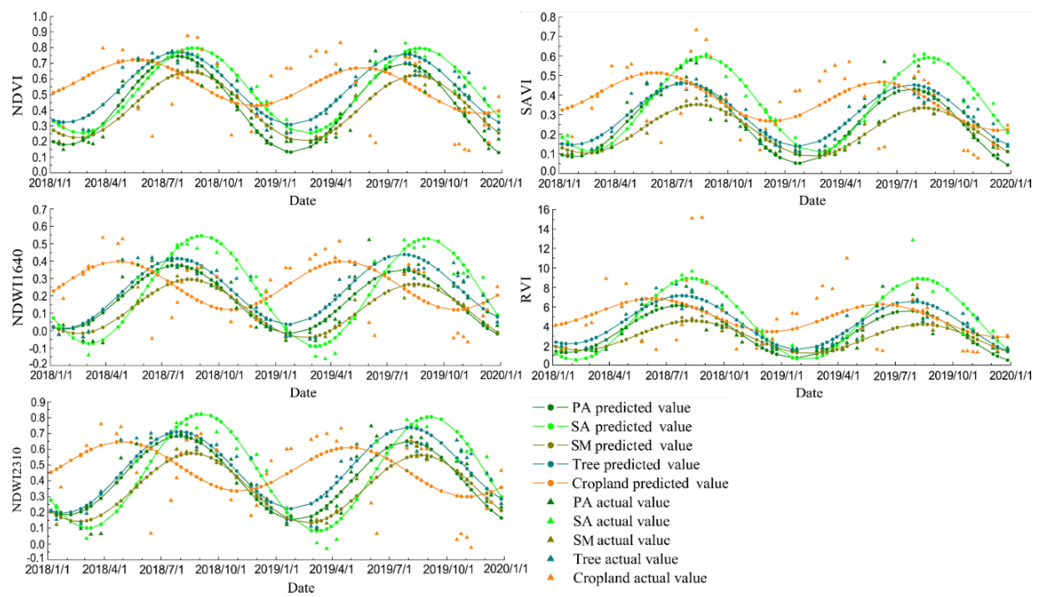
Figure 5.
The actual values and predicted values from the harmonic model of wetland vegetation obtained with Landsat images from 2018 to 2020 for the five VIs.
Figure 5.
The actual values and predicted values from the harmonic model of wetland vegetation obtained with Landsat images from 2018 to 2020 for the five VIs.
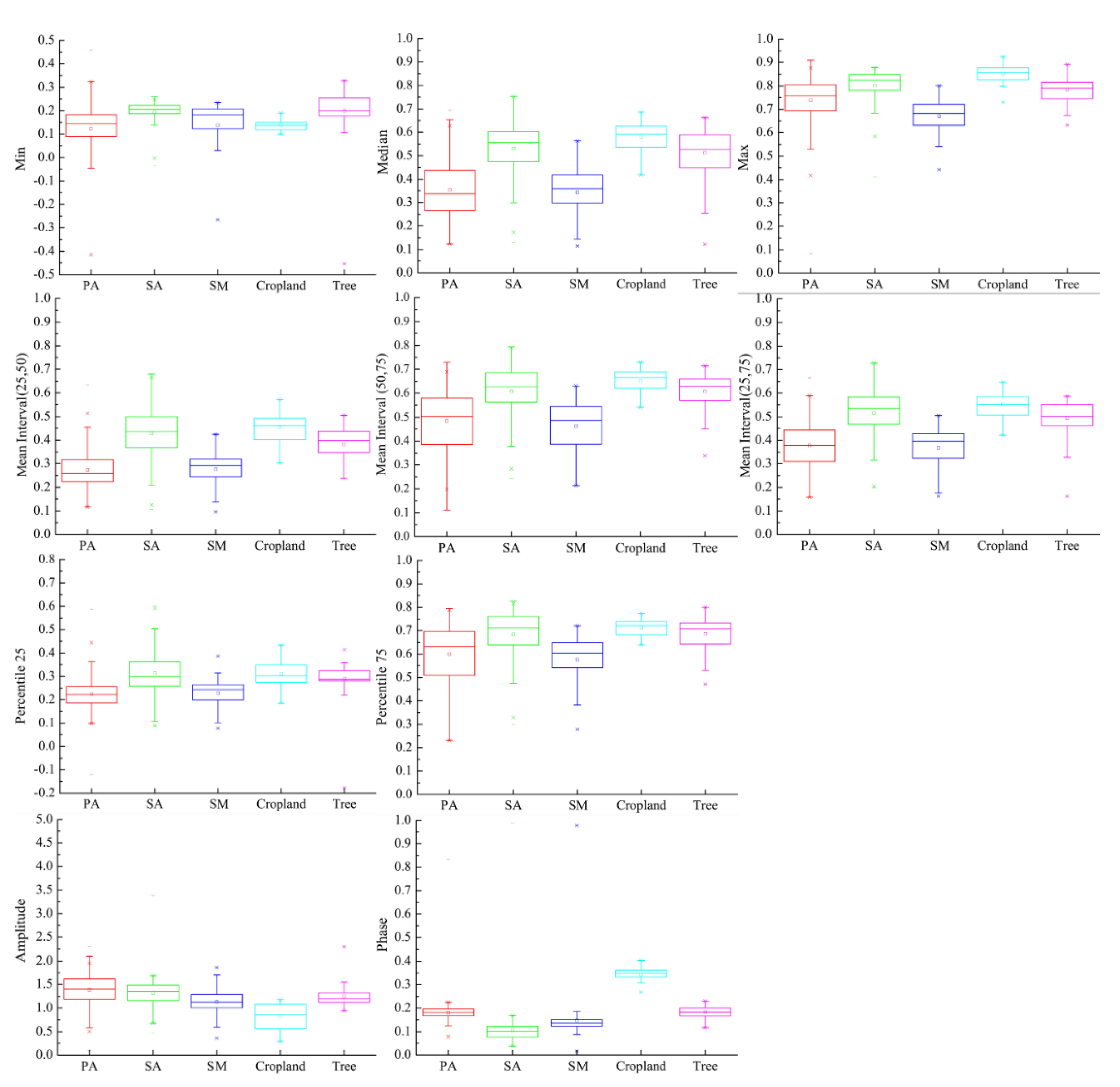
Figure 6.
Differences in NDVI of wetland vegetation in various features. The line in the middle of the box represents the median, the dot in the middle of the box represents the mean value, the top, and bottom of the box represent the 25% and 75% percentiles, respectively; the upper and lower lines represent the maximum and minimum values, respectively; and the points that are discrete outside the box are outliers. The red represents P. australis, green represents S. alterniflora, dark blue represents S. mariqueter, light blue represents cropland, and purple represents trees in the figure.
Figure 7.
Classification considering statistical, temporal, and phenological features. Subfigure (a) shows the Xisha and Niupenggang areas, subfigure (b) shows the Beiliuyao area, and subfigure (c) shows the Dongtan area.
Figure 7.
Classification considering statistical, temporal, and phenological features. Subfigure (a) shows the Xisha and Niupenggang areas, subfigure (b) shows the Beiliuyao area, and subfigure (c) shows the Dongtan area.
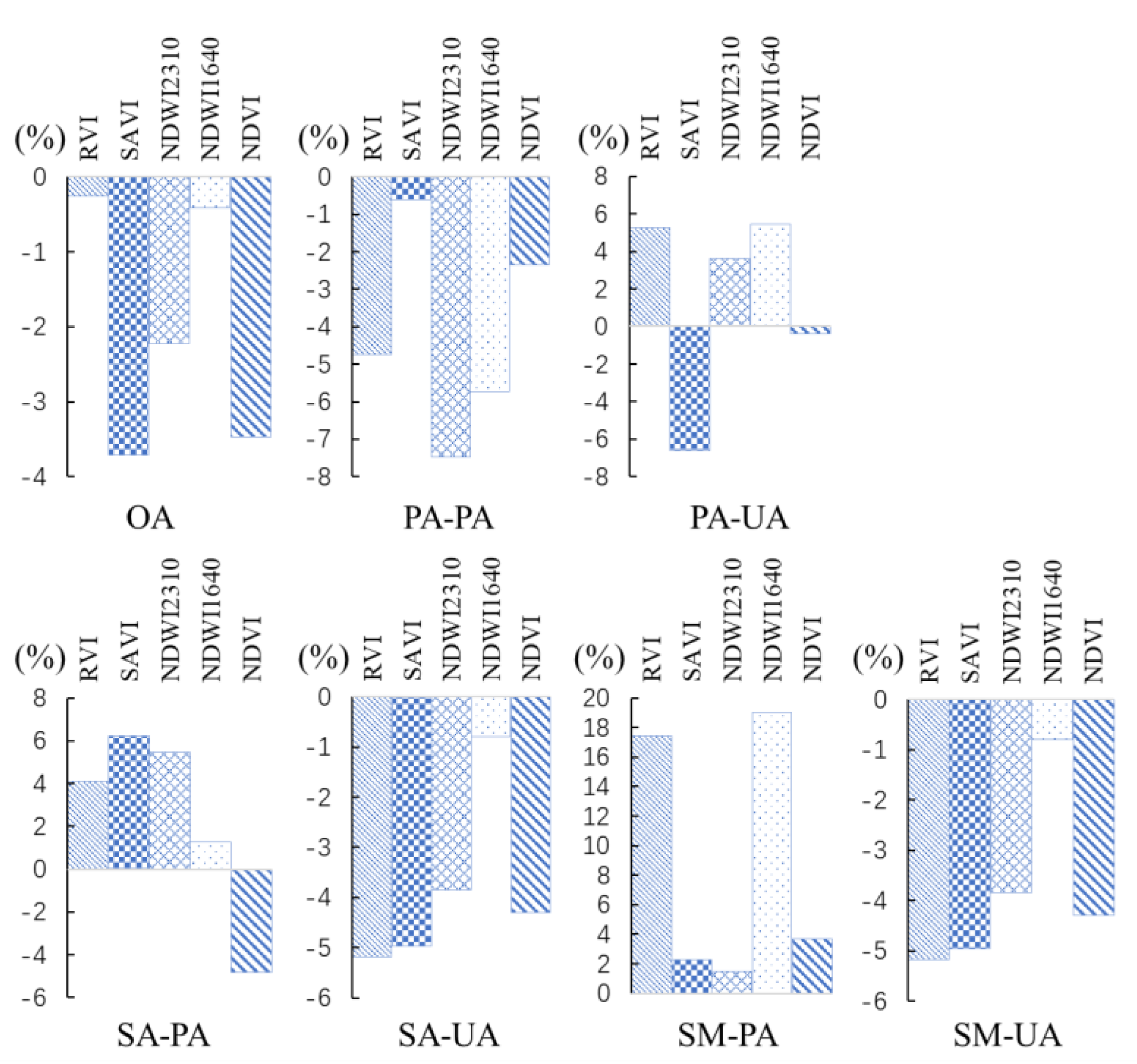
Figure 8.
The percentage changes in classifications accuracy when each kind of VI (NDVI, ratio vegetation index (RVI), soil normalized vegetation index (SAVI), 1640 nm shortwave infrared vegetation index (NDWI1640), and 2310 nm shortwave infrared vegetation index (NDWI2310)) is removed from variable combinations.
Figure 9.
The classification of the senescence period under the proper feature combination. Subfigure (a) shows the Xisha and Niupenggang areas, subfigure (b) shows the Beiliuyao area, and subfigure (c) shows the Dongtan area.
Figure 9.
The classification of the senescence period under the proper feature combination. Subfigure (a) shows the Xisha and Niupenggang areas, subfigure (b) shows the Beiliuyao area, and subfigure (c) shows the Dongtan area.
Figure 10.
The classification of the green period under the proper feature combination. Subfigure (a) shows the Xisha and Niupenggang areas, subfigure (b) shows the Beiliuyao area, and subfigure (c) shows the Dongtan area.
Figure 10.
The classification of the green period under the proper feature combination. Subfigure (a) shows the Xisha and Niupenggang areas, subfigure (b) shows the Beiliuyao area, and subfigure (c) shows the Dongtan area.
Figure 11.
Classification results from the feature collection constructed by Tian et al. Subfigure (a) shows the Xisha and Niupenggang areas, subfigure (b) shows the Beiliuyao area, and subfigure (c) shows the Dongtan area.
Figure 11.
Classification results from the feature collection constructed by Tian et al. Subfigure (a) shows the Xisha and Niupenggang areas, subfigure (b) shows the Beiliuyao area, and subfigure (c) shows the Dongtan area.
Table 1.
Characteristics of the Landsat 8 Operational Land Imager (OLI) images used in the experiment.
Table 1.
Characteristics of the Landsat 8 Operational Land Imager (OLI) images used in the experiment.
| Year | Path | Row | Cloud Cover (%) | Season | Year | Path | Row | Cloud Cover (%) | Season |
|---|
| 2018-01-15 | 118 | 38 | 6.63 | A,S | 2019-01-18 | 118 | 38 | 0.61 | A,S |
| 2018-03-04 | 118 | 38 | 41.44 | A,S | 2019-03-07 | 118 | 38 | 41.75 | A,S |
| 2018-04-21 | 118 | 38 | 77.97 | A,S | 2019-03-23 | 118 | 38 | 15.99 | A,S |
| 2018-05-23 | 118 | 38 | 18.66 | A | 2019-04-08 | 118 | 38 | 41.30 | A,S |
| 2018-06-08 | 118 | 38 | 87.86 | A,G | 2019-05-10 | 118 | 38 | 6.97 | A |
| 2018-06-24 | 118 | 38 | 61.50 | A,G | 2019-06-11 | 118 | 38 | 55.17 | A,G |
| 2018-07-10 | 118 | 38 | 66.41 | A,G | 2019-06-27 | 118 | 38 | 93.79 | A,G |
| 2018-07-26 | 118 | 38 | 5.89 | A,G | 2019-07-29 | 118 | 38 | 10.87 | A,G |
| 2018-08-11 | 118 | 38 | 9.25 | A,G | 2019-08-14 | 118 | 38 | 3.30 | A,G |
| 2018-08-27 | 118 | 38 | 27.05 | A,G | 2019-08-30 | 118 | 38 | 7.94 | A,G |
| 2018-09-28 | 118 | 38 | 16.82 | A,G | 2019-10-17 | 118 | 38 | 54.22 | A |
| 2018-10-30 | 118 | 38 | 7.32 | A | 2019-11-02 | 118 | 38 | 15.12 | A,S |
| 2018-12-01 | 118 | 38 | 20.58 | A,S | 2019-12-04 | 118 | 38 | 6.38 | A,S |
| 2018-12-17 | 118 | 38 | 0.77 | A,S | 2019-01-25 | 119 | 38 | 65.95 | A,S |
| 2018-01-06 | 119 | 38 | 37.59 | A,S | 2019-02-26 | 119 | 38 | 42.47 | A,S |
| 2018-01-22 | 119 | 38 | 42.16 | A,S | 2019-03-14 | 119 | 38 | 96.98 | A,S |
| 2018-02-07 | 119 | 38 | 58.59 | A,S | 2019-03-30 | 119 | 38 | 99.99 | A,S |
| 2018-02-23 | 119 | 38 | 0.99 | A,S | 2019-04-15 | 119 | 38 | 6.15 | A,S |
| 2018-03-11 | 119 | 38 | 46.00 | A,S | 2019-05-01 | 119 | 38 | 28.89 | A |
| 2018-03-27 | 119 | 38 | 8.95 | A,S | 2019-06-02 | 119 | 38 | 38.03 | A,G |
| 2018-04-28 | 119 | 38 | 3.00 | A,S | 2019-07-04 | 119 | 38 | 99.98 | A,G |
| 2018-05-14 | 119 | 38 | 41.22 | A | 2019-08-05 | 119 | 38 | 42.03 | A,G |
| 2018-05-30 | 119 | 38 | 96.37 | A,G | 2019-08-21 | 119 | 38 | 5.85 | A,G |
| 2018-06-15 | 119 | 38 | 21.57 | A,G | 2019-09-06 | 119 | 38 | 76.00 | A,G |
| 2018-07-17 | 119 | 38 | 43.71 | A,G | 2019-09-22 | 119 | 38 | 74.05 | A,G |
| 2018-08-02 | 119 | 38 | 47.29 | A,G | 2019-10-24 | 119 | 38 | 16.52 | A |
| 2018-08-18 | 119 | 38 | 69.70 | A,G | 2019-11-09 | 119 | 38 | 0.15 | A |
| 2018-09-03 | 119 | 38 | 70.83 | A,G | 2019-12-11 | 119 | 38 | 0.20 | A,S |
| 2018-09-19 | 119 | 38 | 60.92 | A,G | 2019-12-27 | 119 | 38 | 5.12 | A,S |
| 2018-10-05 | 119 | 38 | 64.28 | A,G | | | | | |
| 2018-10-21 | 119 | 38 | 70.36 | A | | | | | |
| 2018-11-22 | 119 | 38 | 4.60 | A,S | | | | | |
| 2018-12-24 | 119 | 38 | 2.44 | A,S | | | | | |
Table 2.
Vegetation index (VI) calculation formulas and associated Google Earth Engine (GEE) code.
Table 2.
Vegetation index (VI) calculation formulas and associated Google Earth Engine (GEE) code.
| VIs | Calculation Formula | GEE Code |
|---|
| NDVI [30] | (NIR-RED)/(NIR + RED) | normalizedDifference([‘B5’,’B4’]) |
| NDWI2130 [29] | (NIR-SWIR2130)/(NIR + SWIR2130) | normalizedDifference([‘B5’,’B6’]) |
| NDWI1640 [29] | (NIR-SWIR1640)/(NIR + SWIR1640) | normalizedDifference([‘B5’,’B7’] |
| SAVI [26] | 1.5 × (NIR-RED)/(NIR + RED + 0.5) | Code equation ‘1.5 × (nir-red)/(nir + red + 0.5)’ |
| RVI [28] | NIR/RED | Code equation ‘nir/red’ |
Table 3.
Selection of vegetation index (VI) features.
Table 3.
Selection of vegetation index (VI) features.
| Group | Name | Description | GEE Code |
|---|
| Statistical features | Median | Median of time-series | |
| Max | Maximum of time-series | |
| Min | Minimum of time-series | |
| Temporal features | Percentile 25 | The value at the 25% quartile of the time series | |
| Percentile 75 | The value at the 75% quartile of the time series |
| Mean Interval (25,75) | The mean value of the time series from 25% to 75% | |
| Mean Interval (25,50) | The mean value of the time series from 25% to 50% | |
| Mean Interval (50,75) | The mean value of the time series from 50% to 75% | |
| Phenological features | Amplitude | Amplitude of VI time series filtered by Hants over a period of time | |
| Phase | Phase of VI time series filtered by Hants over a period of time | |
Table 4.
Classifications under three kinds of features and their combinations.
Table 4.
Classifications under three kinds of features and their combinations.
| Accuracy | SF | TF | PF | SF + TF | SF + PF | TF + PF | SF + TF +PF |
|---|
| Number of features | 18 | 25 | 10 | 43 | 28 | 35 | 53 |
| OA (%) | 79.78 | 73.62 | 80.32 | 79.22 | 82.84 | 83.94 | 85.54 |
| P. australis PA (%) | 85.18 | 85.71 | 90.91 | 90.18 | 83.81 | 95.04 | 88.46 |
| P. australis UA (%) | 78.63 | 68.29 | 81.48 | 73.19 | 82.24 | 80.99 | 82.14 |
| S. alterniflora PA (%) | 79.31 | 82.35 | 89.29 | 76.79 | 85.71 | 86.79 | 83.64 |
| S. alterniflora UA (%) | 80.70 | 66.67 | 83.33 | 91.49 | 90.57 | 90.20 | 92.00 |
| S. mariqueter PA (%) | 57.58 | 32.26 | 77.14 | 25.00 | 66.67 | 60.71 | 60.00 |
| S. mariqueter UA (%) | 61.29 | 50.00 | 77.14 | 37.50 | 66.67 | 65.38 | 66.67 |
| Tree PA (%) | 54.17 | 23.08 | 38.09 | 27.78 | 56.52 | 47.62 | 86.67 |
| Tree UA (%) | 76.47 | 54.54 | 100.00 | 55.56 | 61.90 | 76.92 | 81.25 |
| Cropland PA (%) | 62.50 | 11.11 | 100.00 | 75.00 | 100.00 | 100.00 | 83.33 |
| Cropland UA (%) | 100.00 | 50.00 | 66.67 | 100.00 | 100.00 | 100.00 | 100.00 |
| Mudflat PA (%) | 86.87 | 82.69 | 61.54 | 89.13 | 80.00 | 83.64 | 92.68 |
| Mudflat UA (%) | 73.58 | 78.18 | 76.19 | 78.85 | 83.02 | 80.70 | 79.17 |
| Water PA (%) | 87.50 | 87.18 | 81.71 | 88.89 | 94.03 | 81.69 | 89.19 |
| Water UA (%) | 92.10 | 95.77 | 78.82 | 95.52 | 87.50 | 96.67 | 98.51 |
Table 5.
Comparison of classifications among all seasons, the senescence period and the green period.
Table 5.
Comparison of classifications among all seasons, the senescence period and the green period.
| Accuracy | All Seasons | Senescence Period | Green Period |
|---|
| Number of images | 63 | 24 | 26 |
| OA (%) | 85.54 | 81.57 | 78.59 |
| P. australis PA (%) | 88.46 | 88.99 | 93.41 |
| P. australis UA (%) | 82.14 | 78.86 | 72.03 |
| S. alterniflora PA (%) | 83.64 | 72.92 | 76.00 |
| S. alterniflora UA (%) | 92.00 | 87.50 | 90.48 |
| S. mariqueter PA (%) | 60.00 | 50.00 | 51.43 |
| S. mariqueter UA (%) | 66.67 | 75.00 | 75.00 |
Table 6.
Comparison of vegetation-type areas outside the Chongming Island dam extracted for all seasons, the senescence period, and the green period.
Table 6.
Comparison of vegetation-type areas outside the Chongming Island dam extracted for all seasons, the senescence period, and the green period.
| Type | All Seasons (km2) | Senescence Period (km2) | Green Period (km2) |
|---|
| P. australis | 55.30 | 57.47 | 50.10 |
| S. alterniflora | 61.95 | 52.68 | 57.81 |
| S. mariqueter | 20.51 | 10.85 | 18.16 |
| Tree | 5.09 | 8.84 | 2.55 |
| Cropland | 1.56 | 2.07 | 1.53 |
| Total | 144.41 | 131.91 | 130.15 |
Table 7.
Comparison of wetland vegetation extraction by the feature combination method considering phenology and Tian et al.’s method based on pixel phenological composition.
Table 7.
Comparison of wetland vegetation extraction by the feature combination method considering phenology and Tian et al.’s method based on pixel phenological composition.
| Accuracy | The Result of Tian et al. | The Result of the Feature Combination |
|---|
| OA | 78.26 | 85.54 |
| P. australis PA (%) | 84.91 | 88.46 |
| P. australis UA (%) | 77.59 | 82.14 |
| S. alterniflora PA (%) | 73.85 | 83.64 |
| S. alterniflora UA (%) | 88.89 | 92.00 |
| S. mariqueter PA (%) | 80.00 | 60.00 |
| S. mariqueter UA (%) | 80.00 | 66.67 |


