Article

Reduced-Complexity End-to-End Variational Autoencoder for on Board Satellite Image Compression

1
IRIT/INP-ENSEEIHT, University of Toulouse, 31071 Toulouse, France
2
Telecommunications for Space and Aeronautics (TéSA) Laboratory, 31500 Toulouse, France
3
ISAE-SUPAERO, University of Toulouse, 31055 Toulouse, France
4
CNES, 31400 Toulouse, France
5
Thales Alenia Space, 06150 Cannes, France
6
ESA, 2201 AZ Noordwijk, The Netherlands
*
Author to whom correspondence should be addressed.
Submission received: 18 December 2020 / Revised: 21 January 2021 / Accepted: 22 January 2021 / Published: 27 January 2021
(This article belongs to the Special Issue Remote Sensing Data Compression)

Abstract

:
Recently, convolutional neural networks have been successfully applied to lossy image compression. End-to-end optimized autoencoders, possibly variational, are able to dramatically outperform traditional transform coding schemes in terms of rate-distortion trade-off; however, this is at the cost of a higher computational complexity. An intensive training step on huge databases allows autoencoders to learn jointly the image representation and its probability distribution, possibly using a non-parametric density model or a hyperprior auxiliary autoencoder to eliminate the need for prior knowledge. However, in the context of on board satellite compression, time and memory complexities are submitted to strong constraints. The aim of this paper is to design a complexity-reduced variational autoencoder in order to meet these constraints while maintaining the performance. Apart from a network dimension reduction that systematically targets each parameter of the analysis and synthesis transforms, we propose a simplified entropy model that preserves the adaptability to the input image. Indeed, a statistical analysis performed on satellite images shows that the Laplacian distribution fits most features of their representation. A complex non parametric distribution fitting or a cumbersome hyperprior auxiliary autoencoder can thus be replaced by a simple parametric estimation. The proposed complexity-reduced autoencoder outperforms the Consultative Committee for Space Data Systems standard (CCSDS 122.0-B) while maintaining a competitive performance, in terms of rate-distortion trade-off, in comparison with the state-of-the-art learned image compression schemes.

Graphical Abstract

1. Introduction

Satellite imaging has many applications in oceanography, agriculture, biodiversity conservation, forestry, landscape monitoring, geology, cartography or military surveillance [1]. The increasing spectral and spatial resolutions of on board sensors allow obtaining ever-better quality products, at the cost of an increased amount of data to be handled. In this context, on board compression plays a key role to save transmission channel bandwidth and to reduce data-transmission time [2]. However, it is subject to strong constraints in terms of complexity. Compression techniques can be divided into two categories: lossless and lossy compression. Lossless compression is a reversible technique that compresses data without loss of information. The entropy measure, which quantifies the information contained in a source, provides a theoretical boundary for lossless compression, e.g., the lowest attainable compression bit-rate. For optical satellite images, the typical lossless compression rate that can be achieved is less than 3:1 [3]. On the other side, lossy compression achieves high compression rates through transform coding [4] and the optimization of a rate-distortion trade-off. Traditional frameworks for lossy image compression operate by linearly transforming the data into an appropriate continuous-valued representation, quantizing its coefficients independently, and then encoding this discrete representation using a lossless entropy coder. To give on-ground examples, JPEG (Joint Photographic Experts Group) uses a discrete cosine transform (DCT) on blocks of pixels followed by a Huffman coder whereas JPEG2000 [5] uses an orthogonal wavelet decomposition followed by an arithmetic coder. In the context of on board compression, the consultative committee for space data systems (CCSDS), drawing on the on-ground JPEG2000 standard, recommends the use of the orthogonal wavelet transform [6]. However, the computational requirements of the CCSDS have been considerably reduced with respect to JPEG2000, taking into account the significant hardware constraints in payload image processing units of satellites. This work follows the same logic; however in the context of learned image compression. The idea is to propose a reduced-complexity learned compression scheme, considering on board limitations regarding computational resources due to hardware and energy consumption constraints.
In recent years, artificial neural networks appeared as powerful data-driven tools to solve problems previously addressed with model-based methods. Their independence from prior knowledge and human efforts can be regarded as a major advantage. In particular, image processing has been widely impacted by convolutional neural networks (CNNs). CNNs have proven to be successful in many computer vision applications [7] such as classification [8], object detection [9], segmentation [10], denoising [11] and feature extraction [12]. Indeed, CNNs are able to capture complex spatial structures in the images through the convolution operation that exploits local information. In CNNs, linear filters are combined with non-linear functions to form deep learning structures doted of a great approximation capability. Recently, end-to-end CNNs have been successfully employed for lossy image compression [13,14,15,16]. Such architectures jointly learn a non-linear transform and its statistical distribution to optimize a rate-distortion trade-off. They are able to dramatically outperform traditional compression schemes regarding this trade-off; however at the cost of a high computational complexity.
In this paper, we start from the state-of-the-art CNN image compression schemes [13,16] to design a reduced-complexity framework in order to adapt to satellite image compression. Please note that the second one [16] is a sophistication of the first one [13] that leads to higher performance at the cost of an increased complexity, by better adapting to the input image. More precisely, the variational autoencoder [16] allows reaching state-of-the-art compression performance, close to the one of BPG (Better Portable Graphics) [17] at the expense of a considerable increase in complexity with respect to [13], reflected by a runtime increase between 20% and 50% [16]. Our objective is to find an intermediary solution, with similar performance as [16] and similar or lower complexity as [13]. The first step is an assessment of the complexity of these reference frameworks and a statistical analysis of the transforms they learn. The objective is to simplify both the transform derivation and the entropy model estimation. Indeed, apart from a reduction of the number of parameters required for the transform, we propose a simplified entropy model that still preserves the adaptivity to the input image (as in [16]) and thus maintain compression performance.
The paper is organized as follows. Section 2 presents some background on learned image compression and details two interesting frameworks. Section 3 performs a complexity analysis of these frameworks and a statistical analysis of the transform they learn. Based on these analyses, a complexity-reduced architecture is proposed. After a subjective analysis of the resulting decompressed image quality, Section 4 quantitatively assesses the performance of this architecture on a representative set of satellite images. A comparative complexity study is performed and the impact of the different design options on the compression performance is studied, for various compression rates. A discussion regarding the compatibility of the proposed architecture complexity with the current and future satellite resources is then held. Section 5 concludes the paper. The symbols used in this paper are listed in Appendix A.

2. Background: Autoencoder Based Image Compression

Autoencoders were initially designed for data dimension reduction similar to e.g., Principal Component Analysis (PCA) [7]. In the context of image compression, autoencoders are used to learn a representation with low entropy after quantization. When devoted to compression, the autoencoder is composed of an analysis transform and a synthesis transform connected by a bottleneck that performs quantization and coding. Please note that the dequantization process is integrated in the synthesis transform. An auxiliary autoencoder can also be used to infer the probability distribution of the representation as in [16]. In this paper, we focus on two reference architectures: [13] displayed in Figure 1 (left) and [16] displayed in Figure 1 (right).
The first one [13] is composed of a single autoencoder. The second one [16] is composed of a main autoencoder (slightly different than the one in [13]) and of an auxiliary one which aims to infer the probability distribution of the latent coefficients. Recall that the second architecture is an upgraded version of the first one regarding both the design of the analysis and synthesis transforms and the estimation of the entropy model.

2.1. Analysis and Synthesis Transforms

In the main autoencoder (Figure 1 (left) and left column of Figure 1 (right)), the analysis transform G a is applied to the input data x to produce a representation y = G a ( x ) . After the bottleneck, the synthesis transform G s is applied to the quantized representation y ^ to reconstruct the image x ^ = G s ( y ^ ) . These representations are derived through several layers composed of filters each followed by a non-linear activation function. The learned representation is multi-channel (the output of a particular filter is called a channel or a feature) and non-linear. As previously mentioned, the analysis and synthesis transforms proposed in [16] result from improvements (mainly parameter adjustments) of the ones proposed in [13]. Thus, for brevity, the following description focuses on [16]. In [16], the analysis (resp. synthesis) transform G a (resp. G s ) is derived through 3 convolutional layers each composed of N filters with kernel support n × n associated with parametric activation functions called generalized divisive normalizations (GDN) (resp. Inverse Generalized Divisive Normalizations (IGDN)) and a downsampling (resp. upsampling) by a factor 2. These three convolutional layers are linked to the input (resp. output) of the bottleneck by a convolution layer composed of M > N (resp. N) filters with the same kernel support but without activation function. Please note that the last layer of the synthesis transform is composed of M > N filters and leads to the so-called wide bottleneck that offers increased compression performance according to [16,18]. Contrarily to usual parameter-free activation functions (e.g., ReLU, sigmoid,…), GDN and IGDN are parametric functions that implement an adaptive normalization. In a given layer, the normalization operates through the different channels independently on each spatial location of the filter outputs. If v i ( k , l ) denotes the value indexed by ( k , l ) of the output of the ith filter, the GDN output is derived as follows:
G D N ( v i ( k , l ) ) = v i ( k , l ) ( β i + j = 1 N γ i j v j 2 ( k , l ) ) 1 / 2 for i = 1 , , N .
The IGDN is an approximate inverse of the GDN, derived as follows:
I G D N ( v i ( k , l ) ) = v i ( k , l ) β i + j = 1 N γ i j v j 2 ( k , l ) 1 / 2 for i = 1 , , N .
According to Equation (1) (resp. Equation (2)), the GDN (resp. IGDN) for channel i is defined by N + 1 parameters denoted by β i and γ i j for j = 1 , , N (resp. β i and γ i j for j = 1 , , N ). Finally N ( N + 1 ) parameters are required to define the GDN/IGDN in each layer. The learning and the storage of these parameters are required. However, GDN has been shown to reduce statistical dependencies [19,20] and thus it appears particularly appropriate for transform coding. According to [19], the GDN better estimates the optimal transform than conventional activation functions for a wide range of rate-distortion trade-offs. GDN/IGDN, while intrinsically more complex than usual activation functions, are prone to boost the compression performance especially in case of a low number of layers, thus affording a low global complexity for the network.

2.2. Bottleneck

The interface between the analysis transform and the synthesis transform, the so-called bottleneck, is composed of a quantizer that produces the discrete-valued vector y ^ = Q ( y ) , an entropy encoder and its associated decoder. Recall that the dequantization is performed by the synthesis transform G s (and by H s in the case of the variational autoencoder). A standard entropy coding method, such as arithmetic, range or Huffman coding [21,22,23] losslessly compress the quantized data representation by exploiting its statistical distribution. The bottleneck thus requires a statistical model of the quantized learned representation.

2.3. Parameter Learning and Entropy Model Estimation

2.3.1. Loss Function: Rate Distortion Trade-Off

The autoencoder parameters (filter weights, GDN/IGDN parameters and representation distribution model) are jointly learned through the optimization of a loss function involving the rate R ( y ^ ) and the distortion D ( x , x ^ ) between the original image x and the reconstructed image x ^ . The rate-distortion criterion, denoted as J ( x , x ^ , y ^ ) , writes as the weighted sum:
J ( x , x ^ , y ^ ) = λ D ( x , x ^ ) + R ( y ^ ) ,
where λ is a key parameter that tunes the rate-distortion trade-off.
  • The rate R achieved by an entropy coder is lower-bounded by the entropy derived from the actual discrete probability distribution m ( y ^ ) of the quantized vector y ^ . The rate increase comes from the mismatch between the probability model p y ^ ( y ^ ) required for the coder design and m ( y ^ ) . The bit-rate is given by the Shannon cross entropy between the two distributions:
    H ( y ^ ) = E y ^ m l o g 2 p y ^ ( y ^ ) ,
    where means distributed according to. The bit-rate is thus minimized if the distribution model p y ^ ( y ^ ) is equal to the distribution m ( y ^ ) arising from the actual distribution of the input image and from the analysis transform G a . This highlights the key role of the probability model.
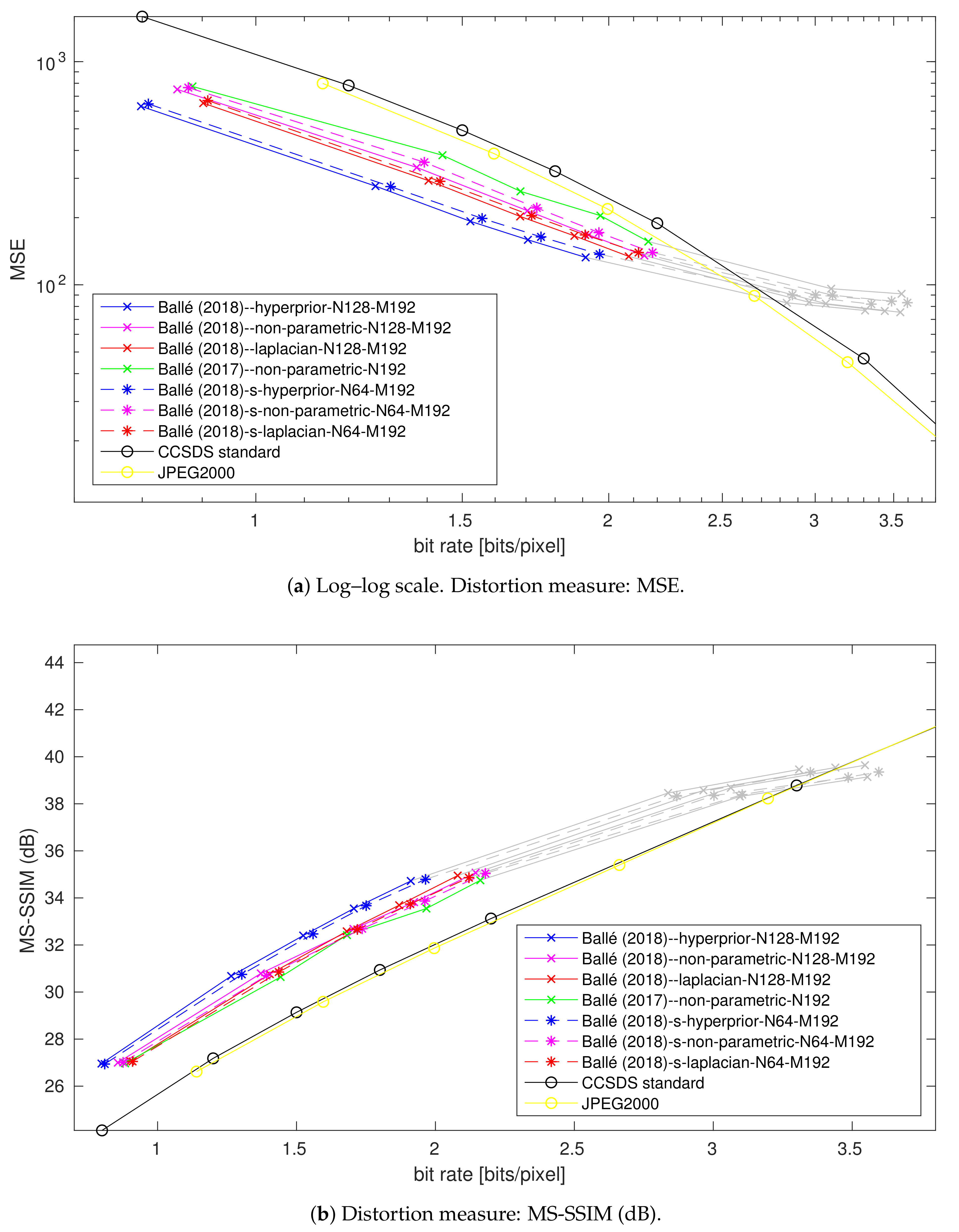
  • The distortion measure D is chosen to account for image quality as perceived by a human observer. Due to its many desirable computational properties, the mean square error (MSE) is generally selected. However, a measure of perceptual distortion may also be employed such as the multi-scale structural similarity index (MS-SSIM) [24].
The loss function defined in Equation (3) is minimized through gradient descent with back-propagation [7] on a representative image training set. However, this requires the loss function to be differentiable. In the specific context of compression, a major hurdle is that the derivative of the quantization function is zero everywhere except at integers, where it is undefined. To overcome this difficulty, a quantization relaxation is considered in the backward pass (i.e., when back-propagating the gradient of the error). Ballé et al. (2016) [13] proposed to back-propagate an independent and identically distributed (i.i.d.) uniform noise, while Theis et al. (2017) [14] proposed to replace the derivative of the quantization function with a smooth approximation. In both cases, the quantization is kept as it is in the forward pass (i.e., when processing an input data).

2.3.2. Entropy Model

As stressed above, a key element in the end-to-end learned image compression frameworks is the entropy model defined through the probability model p y ^ ( y ^ ) assigned to the quantized representation for coding.
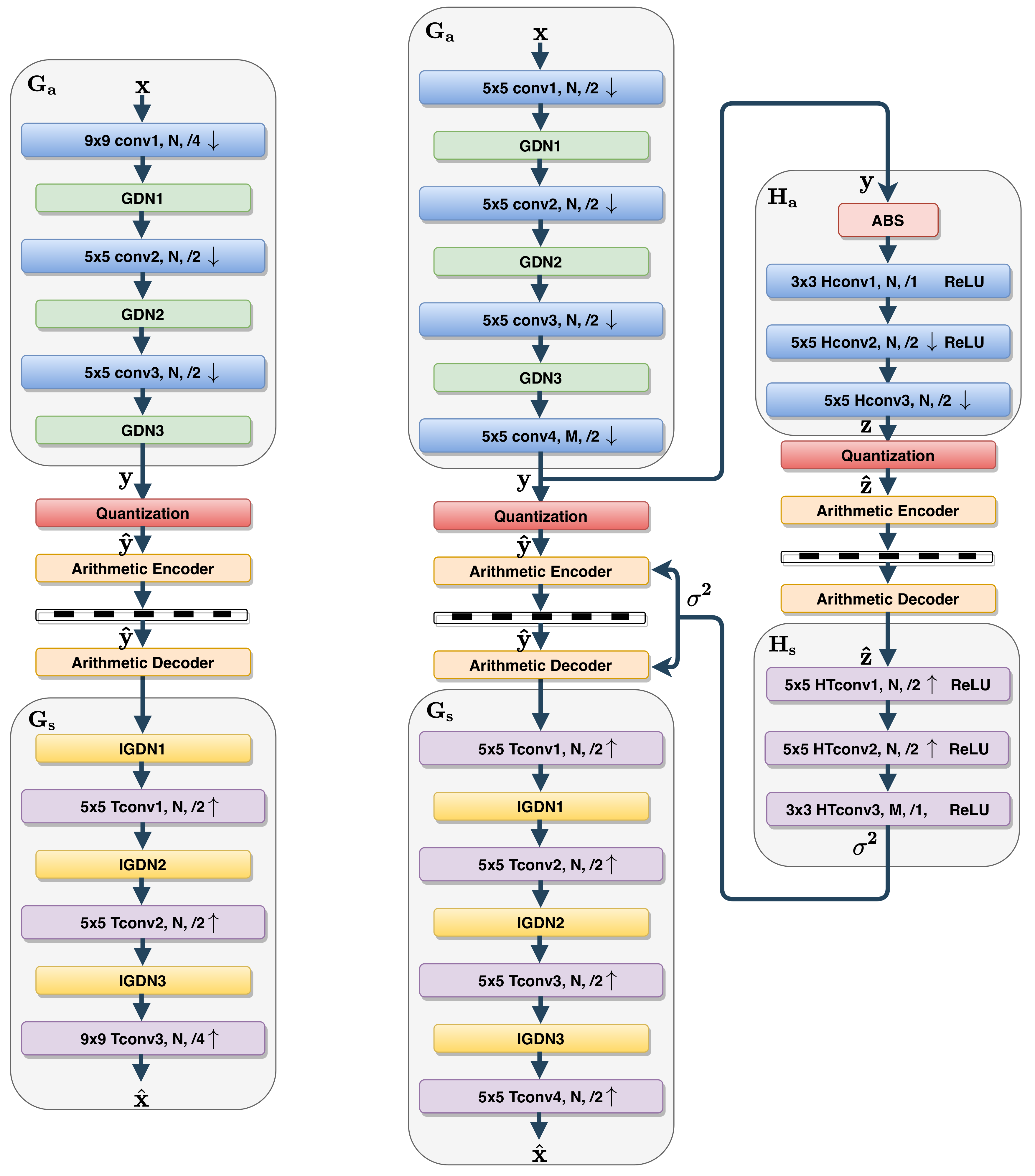
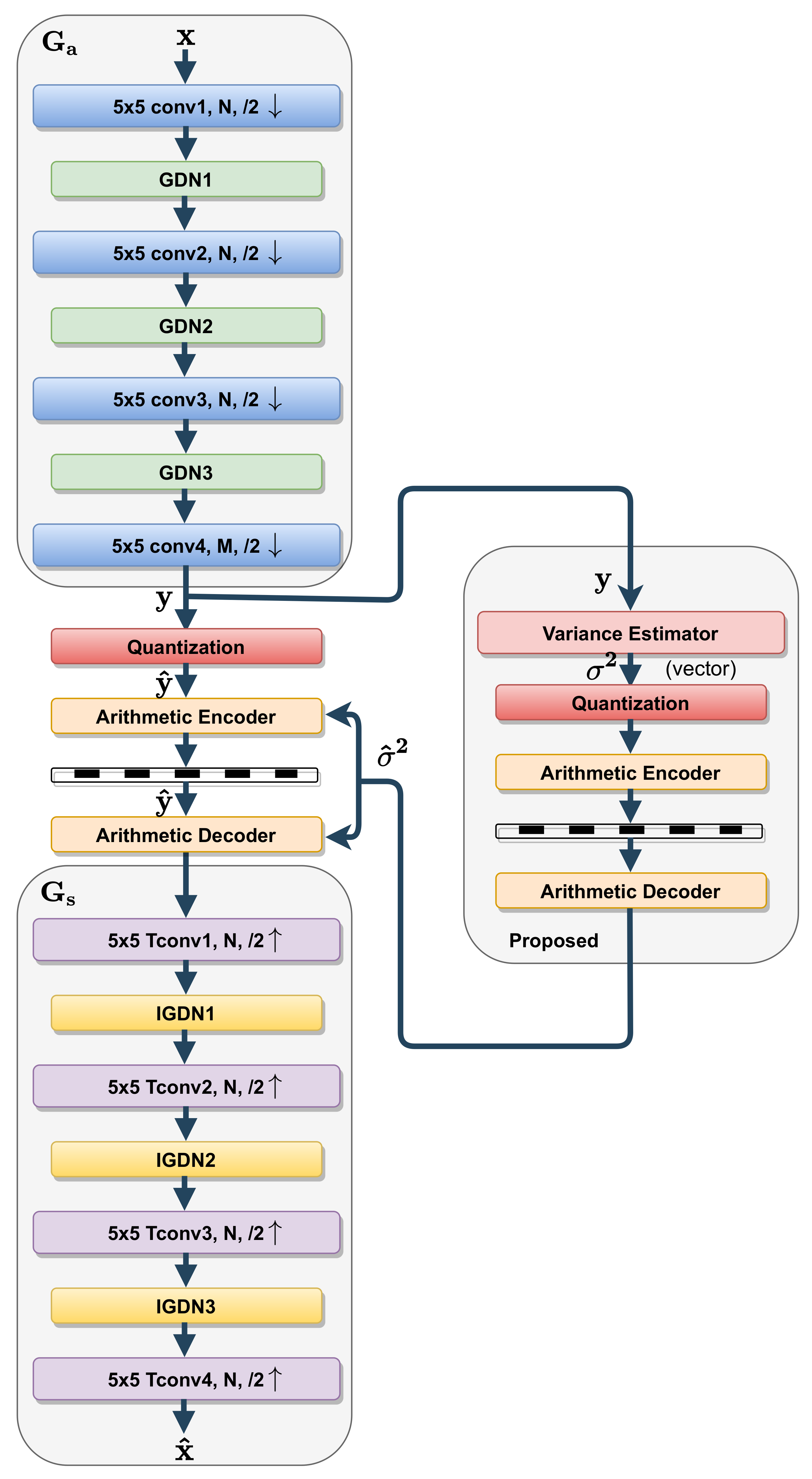
  • Fully factorized model: For simplicity, in [13,14], the approximated quantized representation was assumed independent and identically distributed within each channel and the channels were assumed independent of each other, resulting in a fully factorized distribution:
    p y ˜ | ψ ( y ˜ | ψ ) = i p y ˜ i | ψ ( i ) ( y ˜ i ) ,
    where index i runs over all elements of the representation, through channels and through spatial locations, ψ ( i ) is the distribution model parameter vector associated with each element. As mentioned previously, for back-propagation derivation during the training step, the quantization process ( y ^ = Q ( y ) ) is approximated by the addition of an i.i.d uniform noise Δ y , whose range is defined by the quantization step. Due to the adaptive local normalization performed by GDN non-linearities, the quantization step can be set to one without loss of generality. Hence the quantized representation y ^ , which is a discrete random variable taking values in Z , is modelled by the continuous random vector y ˜ defined by:
    y ˜ = y + Δ y
    taking values in R . The addition of the uniform quantization noise leads to the following expression for p y ˜ i | ψ ( i ) ( y ˜ i ) defined through a convolution by a uniform distribution on the interval 1 / 2 , 1 / 2 :
    p y ˜ i | ψ ( i ) ( y ˜ i ) = p y i | ψ ( i ) y i * U 1 / 2 , 1 / 2 .
    For generality, in [13], the distribution p y i | ψ ( i ) y i is assumed non parametric, namely without predefined shape. In [13,14], the parameter vectors are learned from data during the training phase. This learning, performed once and for all, prohibits adaptivity to the input images during operational phase. Moreover, the simplifying hypothesis of a fully factorized distribution is very strong and not satisfied in practice, elements of y ^ exhibiting strong spatial dependency as observed in [16]. To overcome these limitations and thus to obtain a more realistic and more adaptive entropy model, [16] proposed a hyperprior model, derived through a variational autoencoder, which takes into account possible spatial dependency in each input image.
  • Hyperprior model: Auxiliary random variables z ˜ , conditioned on which the quantized representation y ˜ elements are independent, are derived from y by an auxiliary autoencoder, connected in parallel with the bottleneck (right column of Figure 1 (right)). The hierarchical model hyper-parameters are learned for each input image in operational phase. Firstly, the hyperprior transform analysis H a produces the set of auxiliary random variables z . Secondly, z is transformed by the hyperprior synthesis transform H s into a second set of random variables σ . In [16], z distribution is assumed fully factorized and each representation element y ˜ i , knowing z , is modeled by a zero-mean Gaussian distribution with its own standard deviation σ i . Finally, taking into account the quantization process, the conditional distribution of each quantized representation element is given by:
    y ˜ i | z ˜ N 0 , σ i 2 * U 1 2 , 1 2 .
    The rate computation must take into account the prior distribution of z ˜ , which has to be transmitted to the decoder with the compressed data, as side information.
In the following we derive the complexity of the analysis and synthesis transforms, involved both in the main and in the auxiliary autoencoders of [16]. We also perform a statistical analysis of the learned transform on a representative set of satellite images. The objective is to propose an entropy model simpler while adaptive, because more specifically tailored than the two previous ones.

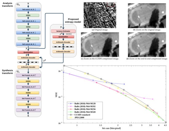
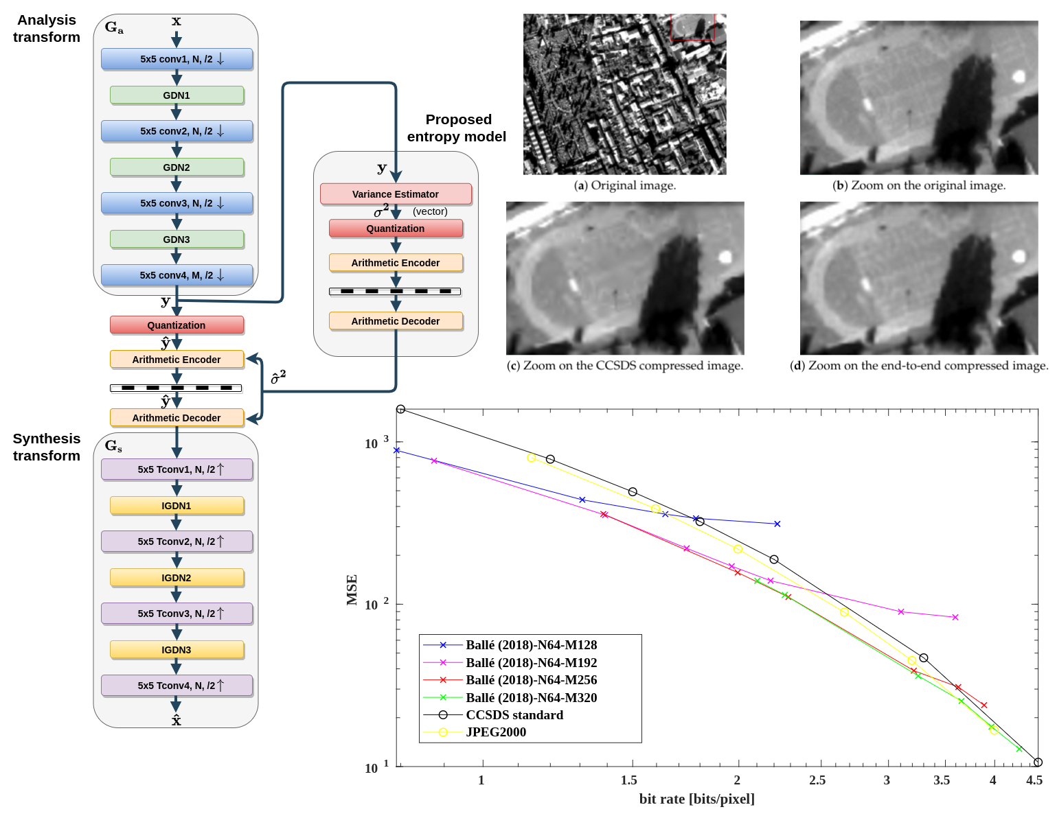
3. Reduced-Complexity Variational Autoencoder

In the literature, the design of learned image compression frameworks hardly takes into account the computational complexity: the objective is merely to obtain the best performance in terms of rate-distortion trade-off. However, in the context of on board compression, a trade-off between performance and complexity has also be considered to take into account the strong computational constraints. Our focus here is to propose a complexity-reduced alternative to the state-of-the-art structure [16] minimizing the impact on the performance. Please note that this complexity reduction must be essentially targeted at the coding part of the framework, most subject to the on board constraints. A meaningful indicator of the complexity reduction is the number of network parameters. Indeed, its reduction has a positive impact not only on the memory complexity, but also on the time complexity and on the training difficulty. Indeed, the optimization problem involved in the training step applies on a smaller number of parameters. This is an advantage even if the training is performed on ground. The convergence is thus obtained with less iterations and thus within a shorter time. Moreover, the complexity reduction has also a positive impact on the ease to upload the final model to the spacecraft (once commissioning is finished and the training with real data completed) as the up-link transmission is severely limited.

3.1. Analysis and Synthesis Transforms

3.1.1. Complexity Assessment

First, let characterize the computational complexity of a convolutional layer composing the analysis and synthesis transforms. Let N i n denote the number of features at the considered layer input. In the particular case of the network first layer, N i n is the number of channels of the input image ( N i n = 1 for a panchromatic image) else N i n is the number of filters of the previous layer. Let N o u t denote the number of features at this layer output, i.e., the number of filters of this layer. As detailed in Section 2, in [16], N o u t = N for each layer of the analysis and synthesis transforms except for the last one of the main auto-encoder analysis transform and the last one of the auxiliary auto-encoder synthesis transform composed of M filters with M > N and thus for these layers N o u t = M . As in [13,16], we consider square filters with size n × n . The number of parameters associated with the filtering part of the layer is:
Param f = ( n × n × N i n + δ ) × N o u t .
The term δ is equal to 1 when a bias is introduced and is equal to 0 otherwise. Please note that this bias is rarely used in the considered architectures (except in Tconv3, as displayed in Figure 1). The filtering is applied to each input channel after downsampling (respectively upsampling). The downsampled (resp. upsampled) input channel if of size s o u t × s o u t with s o u t = s i n / D (respectively s o u t = s i n × D ) where D denotes the downsampling (respectively upsampling) factor and s i n × s i n is the size of a feature at the filter input. Floating points operations Operation f for the filtering operation is thus:
Operation f = Param f × s o u t × s o u t .
GDN/IGDN perform a normalization of a filter output with respect to the other filter outputs. According to Section 2, the number of parameters and the number of operations of each GDN/IGDN are expressed by:
Param g = ( N o u t + 1 ) × N o u t Operation g = Param g × s o u t × s o u t .
Since the number of layers is already very low for the considered architectures, the reduction of the complexity of the analysis and synthesis transforms may target, according to the previous complexity assessment, the number of filters per layer, the size of these filters and the choice of the activation functions. Our proposal below details our strategy for complexity reduction.

3.1.2. Proposal: Simplified Analysis and Synthesis Transforms

Our approach to reduce the complexity of the analysis and synthesis transforms, while maintaining an acceptable rate-distorsion trade-off, is to fine-tune the parameters of each layer (number of filters and filter sizes) and to consider the replacement of GDN/IGDN by simpler non-parametric activation functions.
In a first step, we propose a fine-tuning of the number of filters composing the convolutional layers of the analysis and synthesis transforms. The state-of-the-art frameworks generally involve a large number of filters with the objective of increasing the network approximation capability [13,16]. However, a high number of filters also implies a high number of parameters and operations in the GDN/IGDN, as it increases the depth of the tensors (equal to the number of filters) at their input. Apart from a harder training, a large number of filters comes with a high number of operations as well as a high memory complexity, which is problematic in the context of on board compression. In [16], the number of filters at the bottleneck (M) and for the other layers (N) are fixed according to the target bit-rate: the higher the target bit-rate, the higher M and N. Indeed, higher bit rates mean lower distortion and thus increased network approximation capabilities to learn accurate analysis and synthesis transforms [16]. This principle also applies to the auxiliary autoencoder implementing the hyperprior illustrated in Figure 1 (right column of the right part). In the present paper, we propose and evaluate a reduction of the number of filters in each layer for different target rate ranges. In particular, we investigate the impact of M on the attainable performance when imposing a drastic reduction of N. The question is whether there is a real need for a high global number of filters (high N and M) or whether a high bottleneck size (low N and high M) is sufficient to achieve good performance at high rates. For that purpose, we impose a low value of N (typically N = 64 ) and we consider increasing values of M defined by M = 2 N , 3 N , 4 N , 5 N to determine the minimum value of M that leads to an acceptable performance in a given rate range.
In a second step, we investigate the replacement of the GDN/IGDN by non-parametric activation functions. As previously mentioned, according to [19], GDN/IGDN allow obtaining good performance even with a low number of layers. However, for the sake of completeness, we also test their replacement by ReLU functions. Finally, we propose to evaluate the effect of the filter kernel support. The main autoencoder in [16] is entirely composed of filters with kernel support n × n . The idea then is to test different kernel supports that is ( n 2 ) × ( n 2 ) and ( n + 2 ) × ( n + 2 ) .

3.2. Reduced Complexity Entropy Model

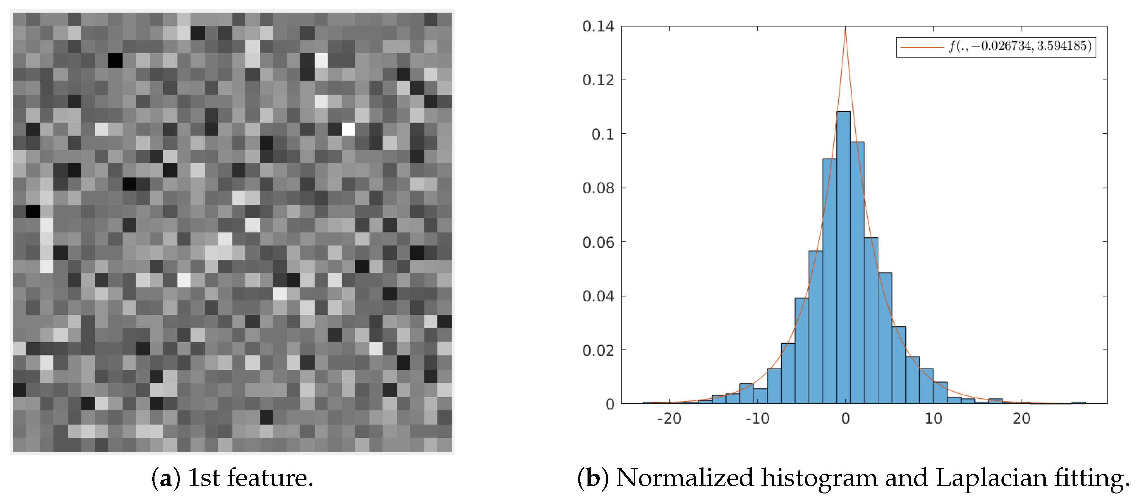
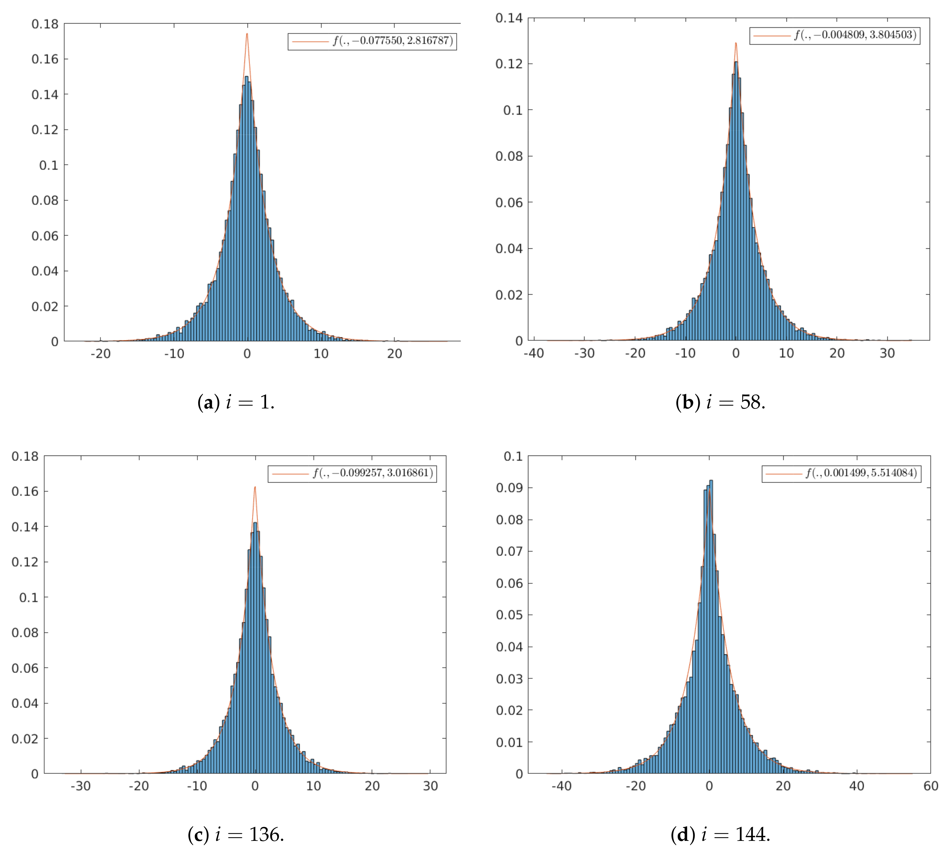
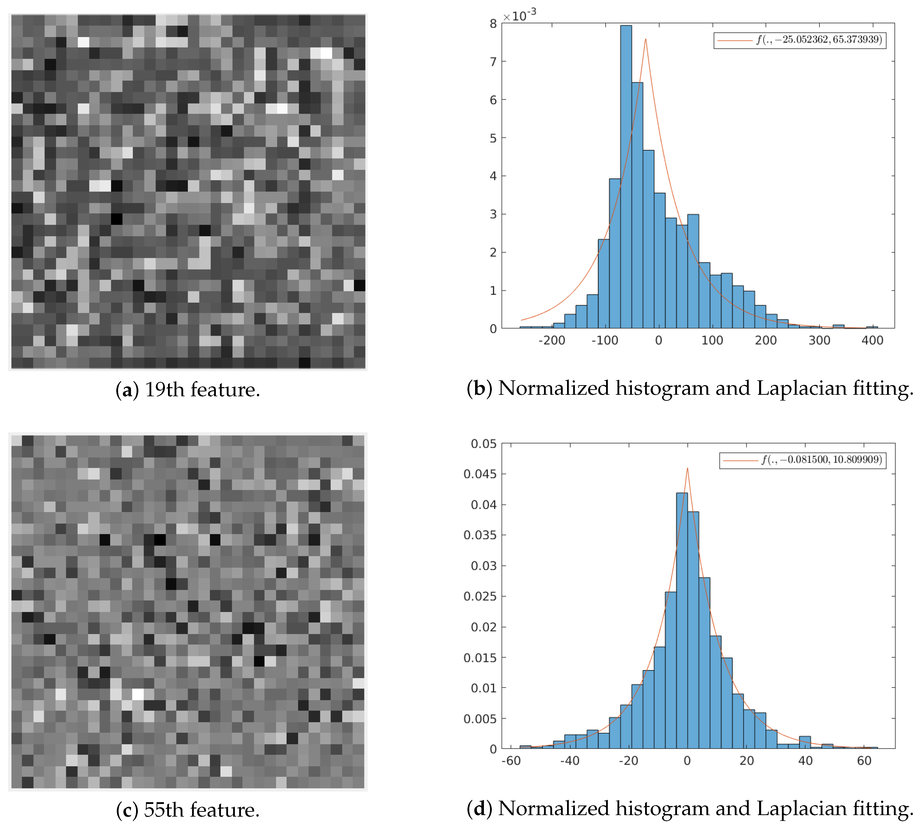
3.2.1. Statistical Analysis of the Learned Transform

This section first performs a statistical analysis of each feature of the learned representation in the particular case of satellite images. A similar statistical analysis has been conducted in the case of natural images in [25] with the objective to properly design the quantization in [13]. The probability density function related to each feature, averaged on a representative set of natural images, was estimated through a normalized histogram. The study showed that most features can be accurately modelled as Laplacian random variables. Interestingly, a similar result has also been analytically demonstrated in [26] for block-DCT coefficients of natural images under the assumption that the variance is constant on each image block and that its values on the different blocks are distributed according to an exponential or a half-normal distribution. We conducted the statistical analysis on the representation obtained by the main autoencoder as defined in [16], with N = 128 and M = 192 , but used alone, as in [13], without auxiliary autoencoder. Indeed, on one side the main autoencoder in [16] benefits from improvements with respect to the one in [13] and on another side, the auxiliary autoencoder is not necessary in this statistical study. This autoencoder is trained on a representative dataset of satellite images and for rates between 2.5 bits / pixel and 3 bits / pixel . First, as an illustration, let consider the satellite image displayed in Figure 2. This image of the city of Cannes (French Riviera) is a 12-bit simulated panchromatic Pléiades image with size. 512 × 512 and resolution 70 cm .
Figure 3 shows the 1st 32 × 32 feature derived from the Cannes image and its normalized histogram with Laplacian fitting.
On this example, the fitting with an almost centered Laplacian seems appropriate. According to the Kolmogorov-Smirnov goodness-of-fit test [27], 94 % of the features derived from this image follow a Laplacian distribution with a significance level α = 5 % . Recall that the Laplacian distribution Laplace ( μ , b ) is defined by:
f ( ζ , μ , b ) = 1 2 b | ζ μ | b for ζ R ,
where μ is the mean value and b > 0 is a scale parameter related to the variance by V a r ( ζ ) = 2 b 2 .
To extend this result, the representation (composed of M = 192 feature maps) was derived for 16 simulated 512 × 512 Pléiades images. Figure 4 shows the normalized histograms (derived from 16 observations) of some feature maps (each of size 32 × 32 ) and the Laplacian fitting.
Most of the feature maps have a similar normalized histogram. According to Kolmogorov-Smirnov goodness-of-fit test [27], 94% of the features derived from this image follow a Laplacian distribution with a significance level α = 5 % . Please note that the Gaussian distribution, N ( μ , σ 2 ) with a small value of μ , also fits the features albeit to a lesser extent. The remaining non-Laplacian feature maps (6% of the maps for this example) stay close to the Laplacian distribution. Figure 5 displays two representative examples of non-Laplacian feature maps. Please note that the first one (19th feature map) is far from Laplacian, this feature appears as a low-pass approximation of the input image. However, this is a very particular case: the second displayed feature has a typical behavior, not so far from a Laplacian distribution.

3.2.2. Proposal: Simplified Entropy Model

The entropy model simplification aims at achieving a compromise between simplicity and performance while preserving the adaptability to the input image. In [13], the representation distribution is assumed fully factorized and the statistical model for each feature is non-parametric to avoid a prior choice of a distribution shape. This model is learned once, during the training. In [16], the strong independence assumption leading to a fully factorized model is avoided by the introduction of the hyperprior distribution, whose parameters are learned for each input image even in the operational phase. Both models are general and thus suitable to a wide variety of images; however the first one implies a strong hypothesis of independence and prohibits adaptivity while the second one is computationally expensive. Based on the previous analysis, we propose the following parametric model for each of the M features. Consider the jth feature elements y i j for i j I j , where I j denotes the set of indexes covering this feature:
y i j Laplace ( 0 , b j ) ( resp . y i j N ( 0 , σ j 2 ) ) with : b j = V a r ( y i j ) / 2 ( resp . σ j 2 = V a r ( y i j ) ) .
The problem then boils down to the estimation of a single parameter per feature referred to as the scale b j (respectively the standard deviation σ j ) in the case of the Laplacian (resp. Gaussian) distribution. Starting from [16], this proposal reduces the complexity at two levels. First, the hyperprior autoencoder, including the analysis H a and synthesis H s transforms, is removed. Second, the side information initially composed of the compressed auxiliary random variable set ( z ) of size 8 × 8 × M now reduces to a M × 1 vector of variances. The auxiliary network simplification is displayed on the right part of Figure 6.
In the next section, the performance of these proposals and of their combinations are studied for different rate ranges.

4. Performance Analysis

This section assesses the performance, in terms of rate-distortion, of the proposed method in comparison with the CCSDS 122.0-B [6], JPEG2000 [5] and with the reference methods [13,16]. Beforehand, a subjective image quality assessment is proposed. Although informal, it allows comparing the artefacts produced by learned compression and by the CCSDS 122.0-B [6].

4.1. Implementation Setup

To assess the relevance of the proposed complexity reductions, experiments were conducted using TensorFlow. The batch size (i.e., the number of training samples to work through before the parameters are updated) was set to 8 and up to 1M iterations were performed. Both training and validation datasets are composed of simulated 12-bit Pléiades panchromatic images provided by the CNES, covering various landscapes (i.e., desert, water, forest, industrial, cloud, port, rural, urban). The reference learned frameworks for image compression are designed to handle 8-bit RGB natural images and they generally target low rates (typically up to a maximum of 1.5 bits/pixel). In contrast, on board satellite compression handles 12-bit panchromatic images and targets higher rates (from 2 bits / pixel to 3.5 bits / pixel ). The training dataset is composed of 8M of patches (of size 256 × 256 ) randomly cropped from 112 images (of size 585 × 585 ). The validation dataset is composed of 16 images (of size 512 × 512 ). MSE was considered to be the distortion metric for training. The rate and distortion measurements were averaged across the validation dataset for a given value of λ . Please note that the value of λ has to be set by trial and error for a targeted rate range.
In addition to the MSE, we also evaluate those results in terms of MS-SSIM. Please note that they exhibit a similar behavior even if the models were trained for the MSE only. The proposed framework is compared with the CCSDS 122.0-B [6], JPEG2000 [5] and with the reference methods [13,16] implemented for values of N and M recommended by their authors for particular rate ranges.
  • Ballé(2017)–non-parametric-N refers to the autoencoder [13] and is implemented for N = 192 (respectively N = 256 ) for rates below 2 bits / pixel (respectively above 2 bits / pixel ).
  • Ballé(2018)–hyperprior-N-M refers to the variational autoencoder [16] and is implemented for N = 128 and M = 192 (respectively N = 192 and M = 320 ) for rates below 2 bits / pixel (respectively above 2 bits / pixel ).

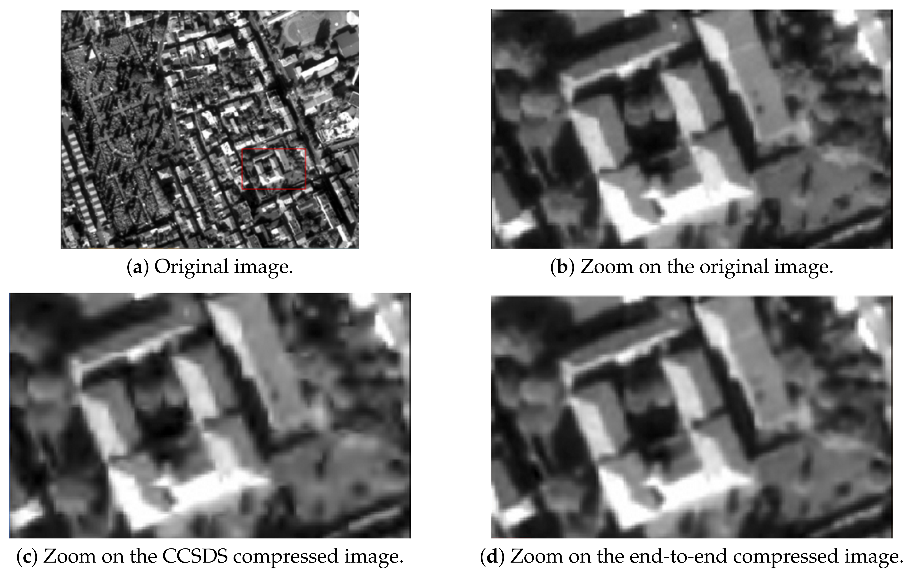
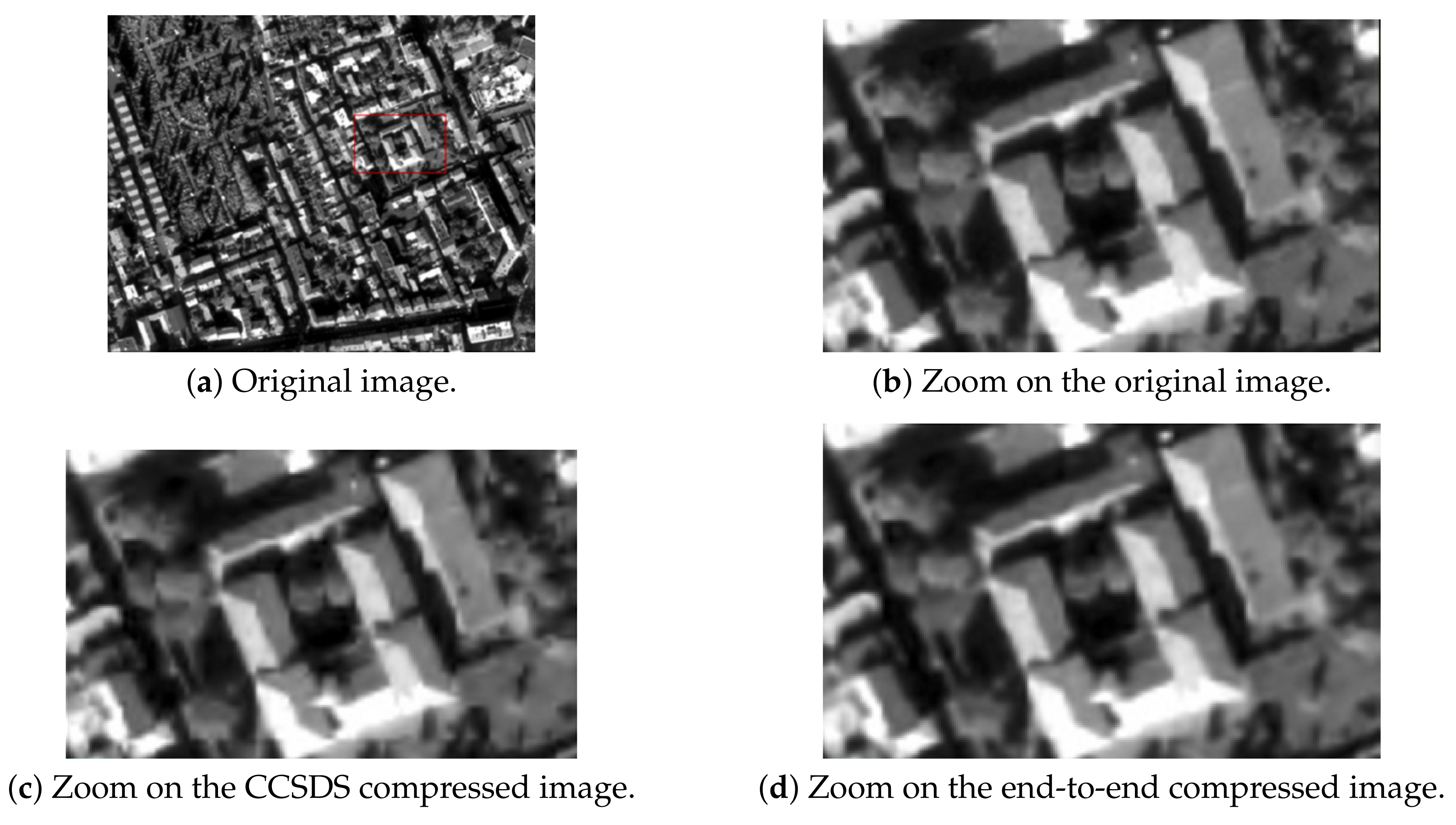
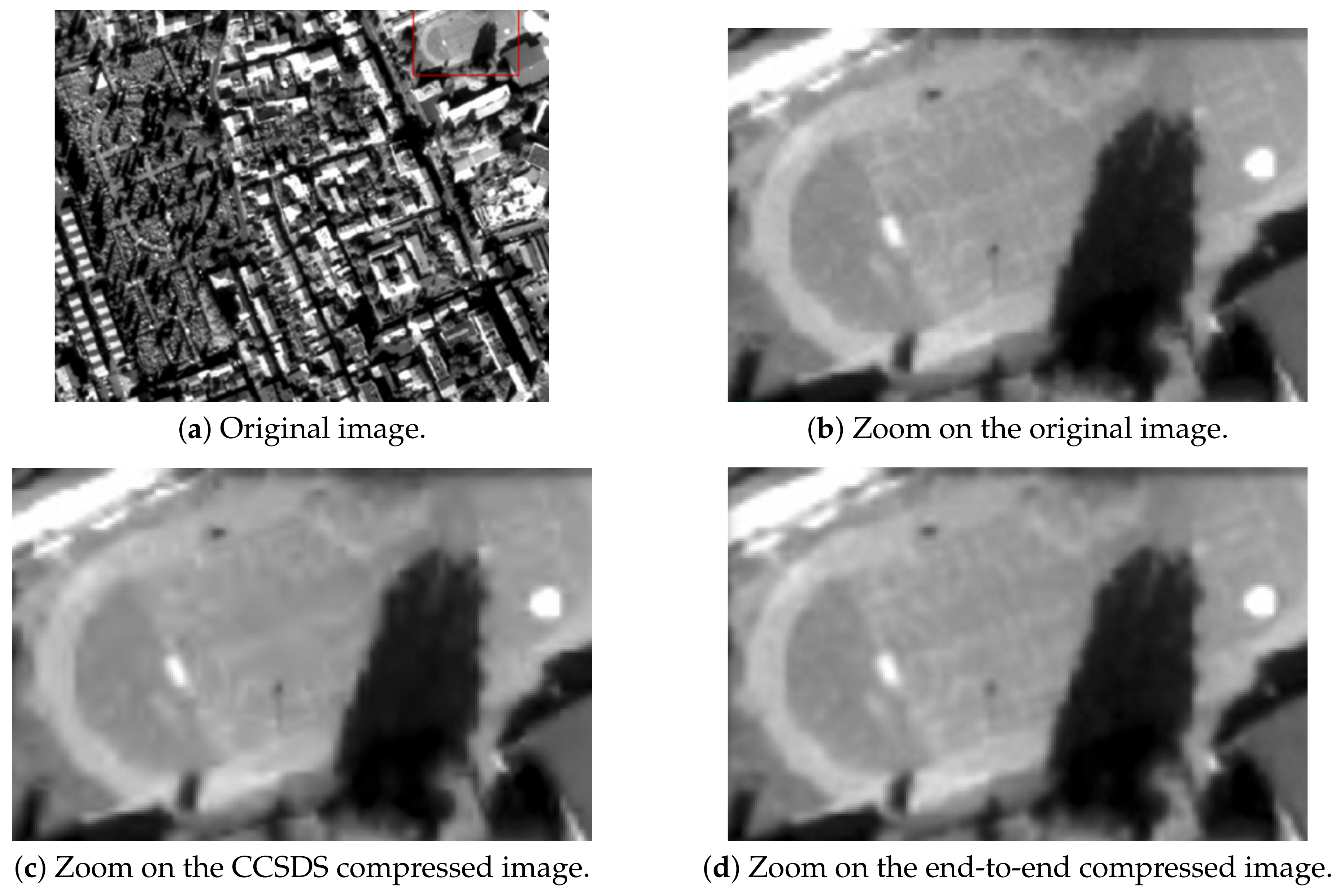
4.2. Subjective Image Quality Assessment

At low rates, JPEG2000 is known to produce quite prominent blurring and ringing artifacts, which is particularly visible in high-frequency textures [5]. This is also the case for the CCSDS 122.0-B [6]. Figure 7a,b shows the original image of the city of Blagnac, which is a 12-bit simulated panchromatic Pléiades image with size 512 × 512 and resolution 70 cm. The figure also shows the image compressed by CCSDS 122.0 (c) and the image compressed by the reference learned compression architecture Ballé(2017)–non-parametric-N (d), for a low compression rate ( 1.15 bits/pixel). The image obtained through learned compression appears closest to the original one than the image obtained through the CCSDS.
For medium luminances, far less artifacts, such as blurring and flattened effects are observed. In particular, the building edges are sharper. The same is true for low luminances, corresponding to shaded areas: the ground markings are sharp and less flatened areas are observed. As shown in Figure 8, for a higher rate of 1.66 bits/pixel, the two reconstructed images are very close. However, the image obtained through learning compression remains closest to the original one, especially in shaded areas.
Finally, as shown in Figure 9 for an even higher rate of 2.02 bits/pixel, CCSDS 122.0 still produces flattened effects, especially in low variance areas. The learned compression method leads to a reconstructed image that is closest to the original one. Even though the stadium ground markings slightly differs from the original, the image quality is overall preserved.
Finally, for various rates, the learned compression method [13] does not suffer from the troublesome artifacts induced by the CCSDS 122.0, leading to a more uniform image quality. The same behavior was observed for the proposed method.
In the following, an objective performance analysis is performed in terms of rate-distortion trade-off for the CCSDS 122.0-B [6], JPEG2000, the reference methods [13,16] and the proposed ones.

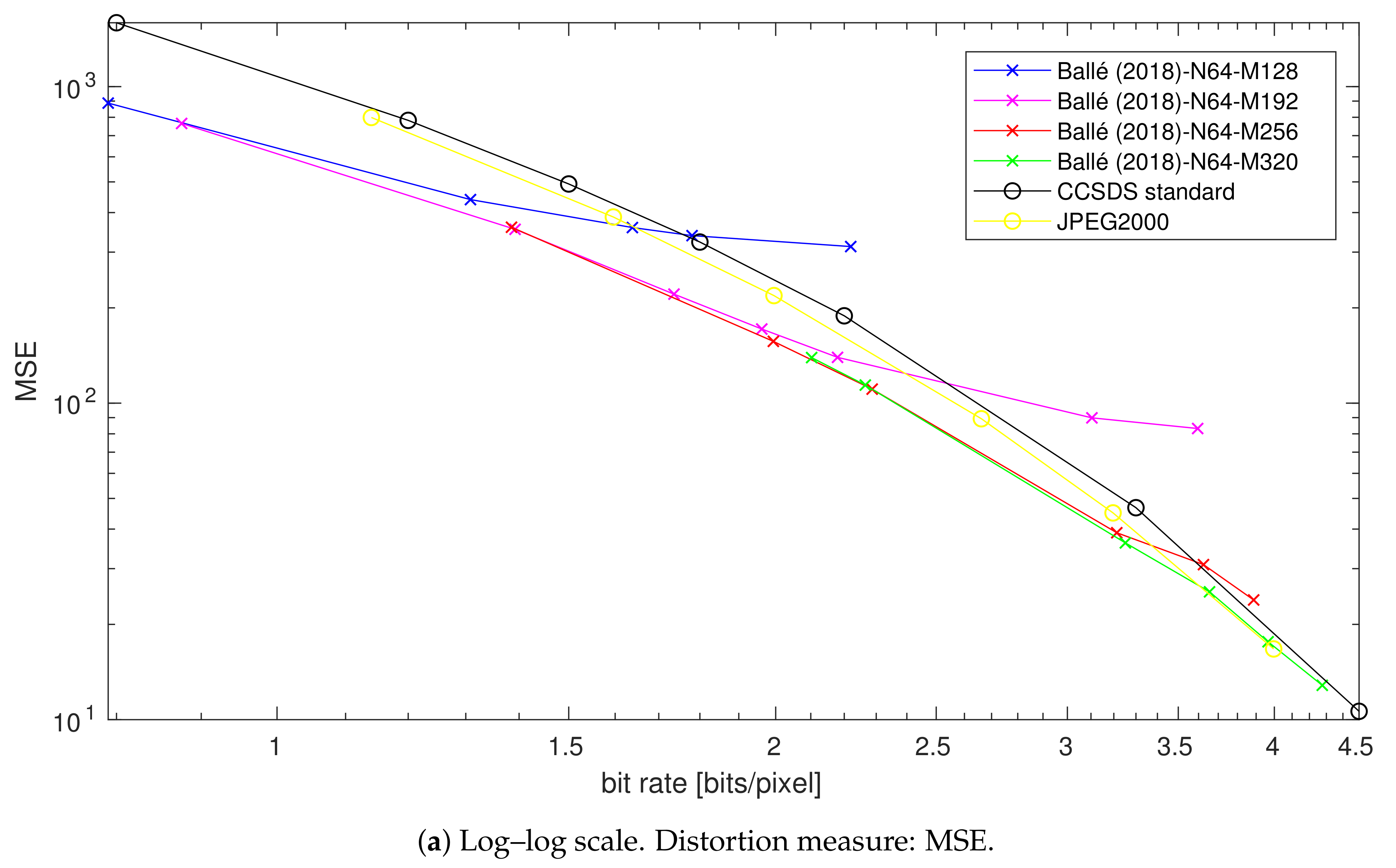
4.3. Impact of the Number of Filter Reduction

4.3.1. At Low Rates

We first consider architectures devoted to low rates, say up to 2 bits/pixel. Starting from [16] denoted as Ballé(2018)–hyperprior-N128-M192, the number of filters N (for all layers, apart from the one just before the bottleneck) is reduced from N = 128 to N = 64 , keeping M = 192 for the layer just before the bottleneck. This reduction is applied jointly to the main autoencoder and to the hyperprior one. The proposed simplified architecture is termed Ballé(2018)-s-hyperprior-N64-M192. The complexity of this model is evaluated in terms of number of parameters and of floating point operation per pixel (FLOPp) in Table 1.
Table 2 compares the complexity of Ballé(2018)-s-hyperprior-N64-M192 to the reference Ballé(2018)-hyperprior-N128-M192.
The complexity of the proposed simplified architecture is 73% lower in terms of FLOPp with respect to the reference method. Now let consider the impact on compression performance of the reduction of N. Figure 10 displays the performance, in terms of MSE and MS-SSIM, of our different proposed solutions, of the reference learned methods and of the JPEG2000 [5] and CCSDS 122.0-B [6] standards. The gray curve portions indicate that the values of N and M are not recommended for this rate range (above 2 bits / pixel ). In this first experiment, we are mainly concerned by the comparison of the blue lines: the solid one for the reference method Ballé(2018)–hyperprior-N128-M192 and the dashed one for the proposal Ballé(2018)–hyperprior-N64-M192.
As expected, Ballé(2018)-s-hyperprior–N64-M192 achieves a rate-distortion performance close to the one of Ballé(2018)–hyperprior-N128-N192 [16], both in terms of MSE and MS-SSIM, for rates up to 2 bits/pixel. We can conclude that the decrease in performance is very small, keeping in mind the huge complexity reduction. Please note that our proposal outperforms by far CCSDS 122.0-B [6], JPEG2000 [5] standards as well as Ballé(2017)-non-parametric-N192 [13].

4.3.2. At High Rates

Now let consider the architecture devoted to higher rates, say above 2 bits/pixel. For such rates, the reference architectures involve a high number of filters ( N = 256 in [13], N = 192 and M = 320 in [16]). Starting from [16], we reduced the number of filters to N = 64 in all layers except the one before the bottleneck, keeping  M = 320 . The proposal Ballé(2018)-s-hyperprior–N64-M320 is compared to the reference Ballé(2018)-hyperprior–N192-M320 but also to Ballé(2017)-non-parametric–N256 and to JPEG2000 [5] and CCSDS 122.0-B [6] standards. Table 3 compares the complexity of Ballé(2018)-s-hyperprior-N64-M320 to the reference Ballé(2018)-hyperprior-N192-M320.
The complexity of the proposed simplified architecture is 87% lower in terms of FLOPp with respect to the reference method. Now let consider the impact on compression performance of the reduction of N. Figure 11 displays the performance, in terms of MSE only, of our different proposed solutions, of the reference learned methods and of the JPEG2000 and CCSDS standards. The MS-SSIM shows the same behaviour.
Theses curves show that the simplified architectures (e.g., resulting from a decrease of N) by far outperform the JPEG2000 and CCSDS standard even at high rates, while showing a low decrease in performance with respect to the reference architectures. Note however that, for both the reference (Ballé(2018)–hyperprior-N192-M320) and the simplified (Ballé(2018)-s-hyperprior-N64-M320) variational models, a training of 1M iterations seems insufficient for the highest rates. Indeed, due to the auxiliary autoencoder implementing the hyperprior, the training has conceivably to be longer, which can be a disadvantage in practice. This may be an additional argument to propose a simplified entropy model.

4.3.3. Summary

As an intermediary conclusion, for either low or high bit rates, a drastic reduction of N starting from the reference architecture [16], does not decrease significantly the performance, both in MSE and in MS-SSIM, while it leads to a complexity decrease of more than 70 % . These results are interesting since it was mentioned in [13,16,19] that structures of reduced complexity would not be able to perform well at high rates.

4.4. Impact of the Bottleneck Size

As previously highlighted, the bottleneck size (M) plays a key role in the performance of the considered architectures. Thus, we now consider a fixed low value of N ( N = 64 ) and then we vary the bottleneck size ( M = 128 , 192 , 256   and   320 ). This experiment, performed on the proposed architecture integrating the simplified entropy model Ballé(2018)-s-laplacian-N64-M, allows quantifying the impact of M on the performance in terms of both MSE and MS-SSIM for increasing values of the target rate. Figure 12 shows the rate-distortion averaged over the validation dataset. According to the literature, high bit rates require a large global number of filters [16].
Figure 12 shows that increasing the bottleneck size M only, while keeping N very small, allows maintaining the performance as the rate increases. As displayed in Figure 12, while the performance reaches a saturation point for a given bottleneck size, it is possible to renew its dynamic by increasing M only. This result is consistent since the number of output channels (M), just before the bottleneck, corresponds to the number of features that must be compressed and transmitted. It therefore makes sense to produce more features at high rates for a better reconstruction of the compressed images. Interestingly, this figure allows establishing in advance the convolution layer dimensions (N and M) for a given rate range, taking into account a complexity concern.

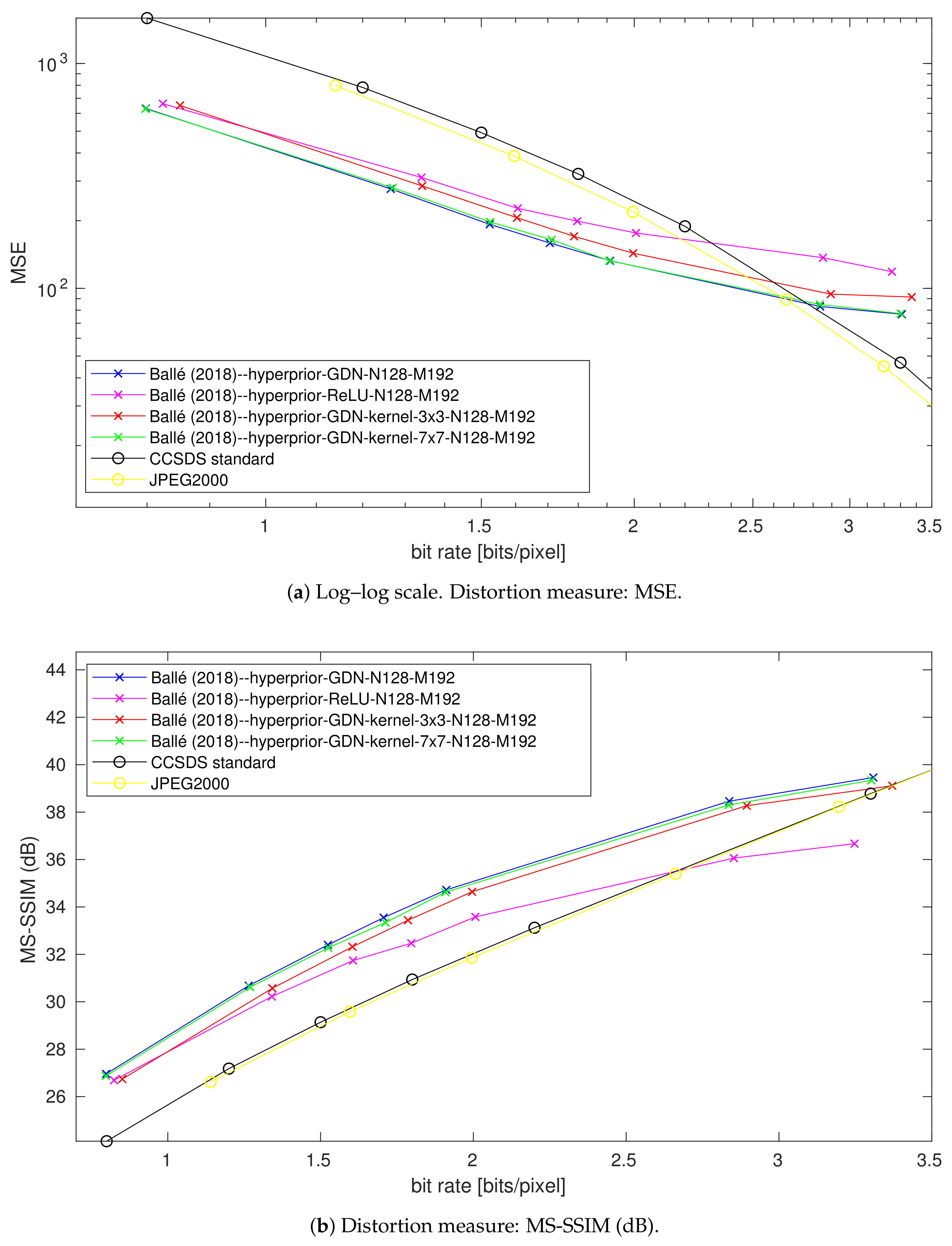
4.5. Impact of the Gdn/Igdn Replacement in the Main Autoencoder

The original architecture Ballé(2018)–hyperprior-N128-M192 of [16], involving GDN/IGDN non-linearities, is compared with the architecture obtained after a full ReLU replacement, except for the last layer of the decoder part. Indeed, this layer involves a sigmoid activation function for constraining the pixel interval mapping between 0 and 1 before the quantization. Figure 13 shows the rate-distortion averaged over the validation dataset in terms of both MSE and MS-SSIM.
As claimed in [19], GDN/IGDN perform better than ReLU for all rates and especially at high rates. Thus, although GDN/IGDN increase the number of parameters to be learned and stored, as well as the number of FLOPp, on one side this increase represents a small percentage of the overall structure with respect to conventional non-linearities [19]. On the other side, GDN/IGDN lead to a dramatic performance boost. In view of these considerations, the complexity reduction in this paper does not target the GDN/IGDN. However, their replacement by simpler activation functions can be envisioned in future work to take into account on board hardware requirements.

4.6. Impact of the Filter Kernel Support in the Main Autoencoder

The original architecture Ballé(2018)–hyperprior-N128-M192 of [16] is also compared when the 5 × 5 filters composing the convolutional layers of the main autoencoder are replaced by 3 × 3 and 7 × 7 filters. It is worth mentioning that all the variant architectures considered in this part share the same entropy model obtained through the same auxiliary autoencoder in terms of number of filters and kernel supports, since the objective here is not to assess the impact of the entropy model. According to Figure 13, a kernel support reduction from 5 × 5 to 3 × 3 leads to a performance decrease. This result is expected in the sense that filters with a smaller kernel support correspond to a reduced approximation capability. On the other hand, a kernel support increase from 5 × 5 to 7 × 7 does not lead to a significant performance improvement. This result indicates that the approximation capability obtained with a kernel support 5 × 5 is sufficient.

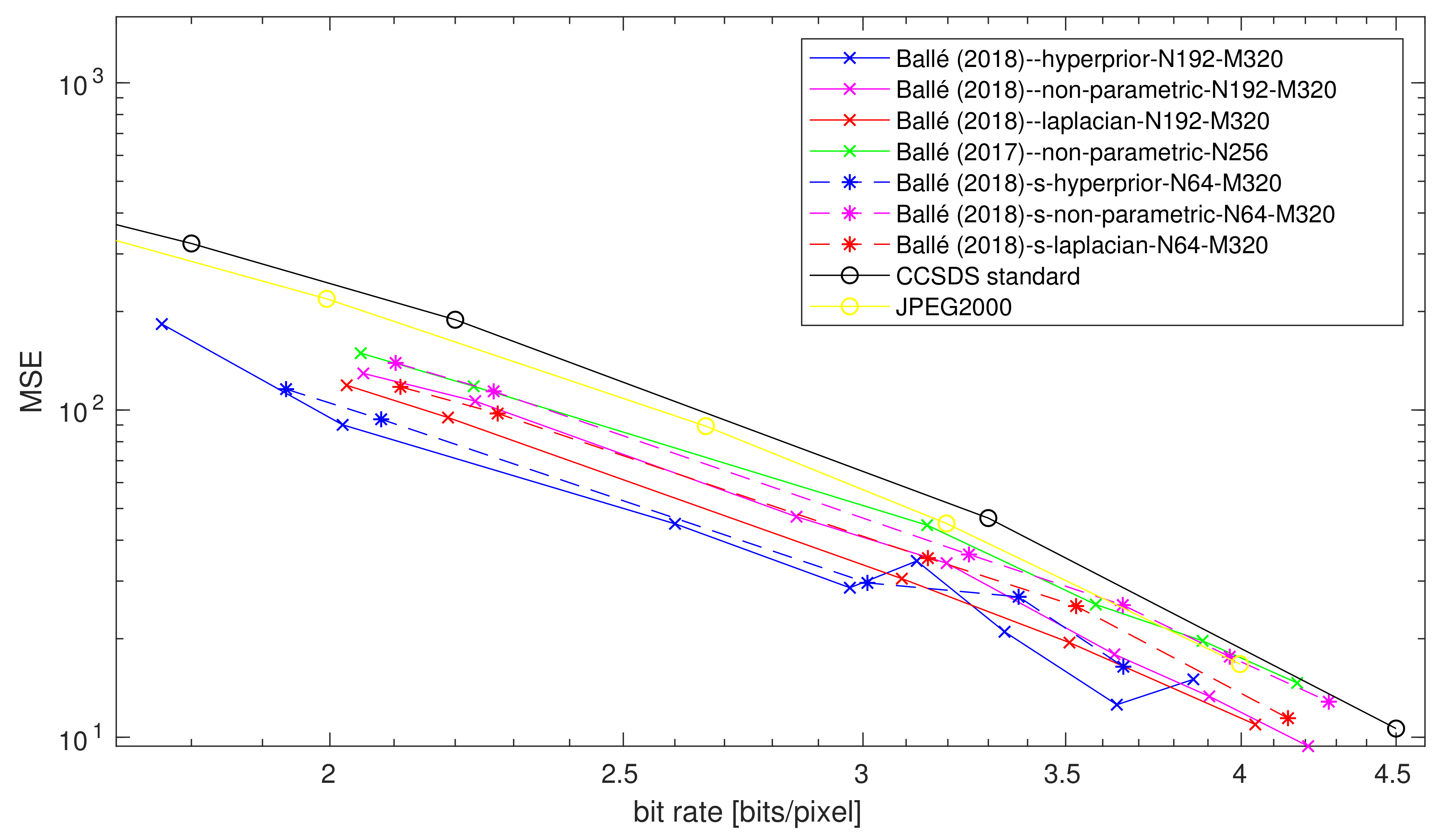
4.7. Impact of the Entropy Model Simplification

4.7.1. At Low Rates

For rates up to 2 bits/pixel, the proposed architectures Ballé(2018)–laplacian-N128-M192 (with the simplified entropy model) and Ballé(2018)-s-laplacian-N64-M192 (combining the reduction of the number of filters to N = 64 and the simplified Laplacian entropy model) are compared with the non-variational reference method Ballé(2017)–non-parametric-N192 [13], with the variational reference method Ballé(2018)–hyperprior-N128-M192 [16], with its version after reduction of the number of filters Ballé(2018)-s-hyperprior-N64-M192, with the architecture denoted as Ballé(2018)-nonparametric-N128-M192 (combining the main auto-encoder in [16] and the non-parametric entropy model in [13]) and its version after reduction of the number of filters Ballé(2018)-s-non-parametric-N64-M192. Table 4 shows that the coding part complexity of Ballé(2018)-s-laplacian-N64-M192 is 13% lower than the one of Ballé(2018)-s-hyperprior-N64-M192.
Figure 10 shows the rate-distortion averaged over the validation dataset for the trained models for both MSE and MS-SSIM quality measures. Recall that the architectures were trained for MSE only. The proposed simplified entropy model (Ballé(2018)-s-laplacian-N64-M192) achieves an intermediate performance between the variational model (Ballé(2018)-s-hyperprior-N64-M192) and the non-variational model (Ballé (2018)-s-non-parametric-N64-M192). Obviously, due to the entropy model simplification, Ballé(2018)-s-laplacian-N64-M192 underperforms the more general and thus more complex Ballé(2018)-s-hyperprior-N64-M192 model. However, the proposed entropy model, even if simpler, preserves the adaptability to the input image, unlike the models Ballé(2018)–non-parametric-N128-M192 and Ballé(2017)–non-parametric-N192 [13]. Please note that the simplified Laplacian entropy model perform close to the hyperprior model at relatively high rates. One possible explanation for this behaviour can be the increased amount of side information required by the hyperprior model [16] for these rates [28].

4.7.2. At High Rates

For high rates (above 2 bits/pixel), the proposed architectures Ballé(2018)–laplacian-N192-M320 (with the simplified entropy model) and Ballé(2018)-s-laplacian-N64-M320 (combining the reduction of the number of filters to N = 64 and the simplified Laplacian entropy model) are compared with the non-variational reference method Ballé(2017)–non-parametric-N256 [13], with the variational reference method Ballé(2018)–hyperprior-N192-M320 [16], with its version after reduction of the number of filters Ballé(2018)-s-hyperprior-N64-M320, with the architecture denoted as Ballé(2018)-nonparametric-N192-M320 (combining the main auto-encoder in [16] and the non-parametric entropy model in [13]) and its version after reduction of the number of filters Ballé(2018)-s-non-parametric-N64-M320. Figure 11 displays the rate-distortion averaged over the validation dataset for the trained models in terms of MSE. The proposed simplified entropy method Ballé(2018)-s-laplacian-N64-M320 achieves an intermediate performance between the variational model (Ballé(2018)-s-hyperprior-N64-M320) and the non-variational model Ballé(2018)-s-non-parametric-N64-M320, similarly to the models targeting lower rates in Figure 10. Table 5 shows that the coding part complexity of Ballé(2018)-s-laplacian-N64-M320 is around 16% lower than the one of Ballé(2018)-s-hyperprior-N64-M320.

4.7.3. Summary

For either low or high bit rates, the proposed entropy model simplication leads to intermediary performance when compared to the reference architectures [13,16], both in MSE and in MS-SSIM, while it leads to a coding part complexity decrease of more than 10 % with respect to [16].

4.8. Discussion About Complexity

According to the previous performance analysis, the computational time complexity of the proposed method is significantly lower than the one of the reference learned compression architecture [16]. However, around 10 kFLOPs/pixel, the attained complexity is at least 2 orders of magnitude higher than the ones of the CCSDS and JPEG2000 [5] standards. Indeed, the complexity of CCSDS 122.0 is around 140 operations per pixel (without optimizations), or 70 MAC (Multiplication Accumulation). The JPEG2000 is 2 to 3 times more complex depending on the optimizations. Note however that the CCSDS 122.0 dates back to 2008 when onboard technologies were limited to radiation-hardened (Rad-Hard) components dedicated to space, with the objectives of 1 Msample/s/W (as specified in the CCSDS 122.0 green book [29]), to process around 50 Mpixels/s. Space technologies, currently developed for the next generation of CNES Earth observation satellites, rather target 5–10 Msample/s/W. Nowadays, the use of commercial off-the-shelf (COTS) components or of dedicated hardware accelerators is envisioned: based on a thinner silicon technology node, they allow higher processing frequencies with consistently lower consumption. For instance, the Movidius Myriade 2 announces 1 TFLOP/s/W. The 10 kFLOP/pixels of the current network would lead to 100 Mpixels/s/W on this component. Therefore, the order of magnitude of the proposed method complexity is not incompatible with an embedded implementation, taking into account the technological leap from the component point of view. Consequently, the complexity increase with respect to the CCSDS one, which we limited as far as possible, is expected to be affordable after computation device upgrading. Please note that, in addition, manufacturers of components dedicated to neural networks provide software suites (for example Xilinx) to optimize the portings. Finally, before on board implementation, a network compression (including pruning, quantization, or tensor decomposition for instance) can be envisioned. However, this is out of the scope of this paper.

5. Conclusions

This paper proposed different solutions to adapt the reference learned image compression models [13,16] to on board satellite image compression, taking into account their computational complexity. We first performed a reduction of the number of filters composing the convolutional layers of the analysis and synthesis transforms, applying a special treatment to the bottleneck. The impact of the bottleneck size, under a drastic reduction of the overall number of filters, was investigated. This study allowed identifying the lowest global number of filters for each rate. For the sake of completeness, we also called into question the other design options of the reference architectures, and especially the parametric activation functions. Second, in order to simplify the entropy model, we also performed a statistical analysis of the learned representation. This analysis showed that most features follow a Laplacian distribution. We thus proposed a simplified parametric entropy model, involving a single parameter. To preserve the adaptivity and thus the performance, this parameter is estimated in the operational phase for each feature of the input image. This entropy model, although far simpler than non-parametric or hyperprior models, brings comparable performance. In a nutshell, by combining the reduction of the global number of filters, and the simplification of the entropy model, we developed a reduced-complexity compression architecture for satellite images that outperforms the CCSDS 122.0-B [6], in terms of rate-distortion trade-off, while maintaining a competitive performance for medium to high rates in comparison with the reference learned image compression models [13,16]. Thereupon, while more complex than traditional CCSDS 122.0 and JPEG 2000 standards, the proposed solutions offer a good compromise between complexity and performance. Thus, we can recommend their use, subject to the availability of suitable on board devices. Besides, future work will be devoted to hardware considerations regarding the on board implementation.

Author Contributions

Conceptualization, M.C. (Marie Chabert), T.O. and C.P.; Formal Analysis, M.C. (Marie Chabert); Investigation, V.A.d.O.; Methodology, V.A.d.O., M.C. (Marie Chabert), T.O. and C.P.; Resources, M.B., C.L., M.C. (Mikael Carlavan), S.H., F.F. and R.C.; Software, V.A.d.O.; Supervision, M.C. (Marie Chabert), T.O. and C.P.; Validation, M.B., C.L., M.C. (Mikael Carlavan), S.H., F.F. and R.C.; Writing—original draft, V.A.d.O. and M.C. (Marie Chabert); Writing—review & editing, T.O. and C.P. All authors have read and agreed to the published version of the manuscript.

Funding

This work has been carried out under the financial support of the French space agency CNES and Thales Alenia Space. Part of this work has been funded by the Institute for Artificial and Natural Intelligence Toulouse (ANITI) under grant agreement ANR-19-PI3A-0004.

Data Availability Statement

Restrictions apply to the availability of these data. Data was obtained from CNES as partner of this study.

Acknowledgments

Experiments presented in this paper were carried out using the OSIRIM platform that is administered by IRIT and supported by CNRS, the Region Midi-Pyrenées, the French Government, ERDF (see http://osirim.irit.fr/site/en).

Conflicts of Interest

The authors declare no conflict of interest.

Abbreviations

The following abbreviations are used in this manuscript:
CCSDSConsultative committee for space data systems
CNNConvolutional neural networks
DCTDiscrete cosine transform
GDNGeneralized divisive normalization
IGDNInverse generalized divisive normalization
JPEGJoint photographic experts group
MSEMean square error
MS-SSIMMulti-scale structural similarity index
PCAPrincipal component analysis
ReLURectified Linear Unit

Appendix A. Table of Symbols Used

This annex tabulates symbols used in this article.
Table A1. Quantities.
SymbolMeaningReference
x original imageSection 2.1
G a ( x ) analysis transformSection 2.1
y learned representationSection 2.1
y ^ quantized learned representationSection 2.1
G s ( y ^ ) synthesis transformSection 2.1
x ^ reconstructed imageSection 2.1
GDNgeneralized divisive normalizationsSection 2.1
IGDNinverse generalized divisive normalizationsSection 2.1
Nfilters composing the convolutional layersSection 2.1
n × n kernel supportSection 2.1
Mfilters composing the last layer of G a Section 2.1
k , l coordinate indexes of the output of the ith filterSection 2.1
v i ( k , l ) value indexed by ( k , l ) of the output of the ith filterSection 2.1
Q ( y ) quantizerSection 2.2
Jrate-distortion loss functionSection 2.3.1
R ( y ^ ) rateSection 2.3.1
D ( x , x ^ ) distortion between the original image x and the reconstructed image x ^ Section 2.3.1
λ parameter that tunes the rate-distortion trade-offSection 2.3.1
m ( y ^ ) actual discrete probability distributionSection 2.3.1
p y ^ ( y ^ ) probability model assigned to the quantized representationSection 2.3.1
H ( y ^ ) bit-rate given by the Shannon cross entropySection 2.3.1
ψ ( i ) distribution model parameter vector associated with each elementSection 2.3.2
Δ y i.i.d uniform noiseSection 2.3.2
y ˜ continuous approximated quantized learned representationSection 2.3.2
z set of auxiliary random variablesSection 2.3.2
H a ( y ) hyperprior analysis transformSection 2.3.2
H s ( z ^ ) hyperprior synthesis transformSection 2.3.2
σ i standard deviation of a zero-mean Gaussian distributionSection 2.3.2
N i n number of features at the considered layer inputSection 3.1.1
N o u t number of features at the considered layer outputSection 3.1.1
Param f number of parameters associated with the filtering part of the considered layerSection 3.1.1
δ term accounting for the biasSection 3.1.1
Ddownsampling factorSection 3.1.1
s i n channel input sizeSection 3.1.1
s o u t downsampled input channel sizeSection 3.1.1
Operation f number of floating points operationsSection 3.1.1
Param g number of parameters associated with each IGDN/GDNSection 3.1.1
Operation g number of floating points operations of each GDN/IGDNSection 3.1.1
ζ random variable that follows a Laplacian distributionSection 3.2.1
μ mean value of a Laplacian distributionSection 3.2.1
bscale parameter of a Laplacian distributionSection 3.2.1
V a r ( ζ ) variance of a laplacian distributed random variableSection 3.2.1
y i feature map elementsSection 3.2.2
I j set of indexes covering the jth featureSection 3.2.2

References

  1. Yu, G.; Vladimirova, T.; Sweeting, M.N. Image compression systems on board satellites. Acta Astronaut. 2009, 64, 988–1005. [Google Scholar] [CrossRef]
  2. Huang, B. Satellite Data Compression; Springer Science & Business Media: New York, NY, USA, 2011. [Google Scholar]
  3. Qian, S.E. Optical Satellite Data Compression and Implementation; SPIE Press: Bellingham, WA, USA, 2013. [Google Scholar]
  4. Goyal, V.K. Theoretical foundations of transform coding. IEEE Signal Process. Mag. 2001, 18, 9–21. [Google Scholar] [CrossRef] [Green Version]
  5. Taubman, D.; Marcellin, M. JPEG2000 Image Compression Fundamentals, Standards and Practice; Springer Publishing Company: New York, NY, USA, 2013. [Google Scholar]
  6. Book, B. Consultative Committee for Space Data Systems (CCSDS), Image Data Compression CCSDS 122.0-B-1, Ser. Blue Book; CCSDS: Washington, DC, USA, 2005. [Google Scholar]
  7. Bengio, Y. Learning deep architectures for AI. Found. Trends Mach. Learn. 2009, 2, 1–127. [Google Scholar] [CrossRef]
  8. Hu, J.; Shen, L.; Sun, G. Squeeze-and-excitation networks. In Proceedings of the 2018 IEEE Conference on Computer Vision and Pattern Recognition (CVPR), Salt Lake City, UT, USA, 18–22 June 2018; pp. 7132–7141. [Google Scholar]
  9. Redmon, J.; Divvala, S.; Girshick, R.; Farhadi, A. You only look once: Unified, real-time object detection. In Proceedings of the 2016 IEEE Conference on Computer Vision and Pattern Recognition (CVPR), Las Vegas, NV, USA, 27–30 June 2016; pp. 779–788. [Google Scholar]
  10. Kaiser, P.; Wegner, J.D.; Lucchi, A.; Jaggi, M.; Hofmann, T.; Schindler, K. Learning aerial image segmentation from online maps. IEEE Trans. Geosci. Remote. Sens. 2017, 55, 6054–6068. [Google Scholar] [CrossRef]
  11. Zhang, K.; Zuo, W.; Chen, Y.; Meng, D.; Zhang, L. Beyond a gaussian denoiser: Residual learning of deep CNN for image denoising. IEEE Trans. Image Process. 2017, 26, 3142–3155. [Google Scholar] [CrossRef] [PubMed] [Green Version]
  12. Wiatowski, T.; Bölcskei, H. A mathematical theory of deep convolutional neural networks for feature extraction. IEEE Trans. Inf. Theory 2017, 64, 1845–1866. [Google Scholar] [CrossRef] [Green Version]
  13. Ballé, J.; Laparra, V.; Simoncelli, E. End-to-end optimized image compression. In Proceedings of the International Conference on Learning Representations (ICLR), Toulon, France, 24–26 April 2017. [Google Scholar]
  14. Theis, L.; Shi, W.; Cunningham, A.; Huszár, F. Lossy image compression with compressive autoencoders. In Proceedings of the International Conference on Learning Representations (ICLR), Toulon, France, 24–26 April 2017. [Google Scholar]
  15. Rippel, O.; Bourdev, L. Real-Time Adaptive Image Compression. In Proceedings of the International Conference on Machine Learning (ICML), Sydney, Australia, 6–11 August 2017; pp. 2922–2930. [Google Scholar]
  16. Ballé, J.; Minnen, D.; Singh, S.; Hwang, S.J.; Johnston, N. Variational image compression with a scale hyperprior. In Proceedings of the International Conference on Learning Representations (ICLR), Vancouver, BC, Canada, 30 April–3 May 2018. [Google Scholar]
  17. Bellard, F. BPG Image Format. 2015. Available online: https://bellard.org/bpg (accessed on 15 December 2020).
  18. Cheng, Z.; Sun, H.; Takeuchi, M.; Katto, J. Deep Residual Learning for Image Compression. In Proceedings of the 2019 IEEE Conference on Computer Vision and Pattern Recognition Workshops, Long Beach, CA, USA, 16–20 June 2019. [Google Scholar]
  19. Ballé, J. Efficient Nonlinear Transforms for Lossy Image Compression. In Proceedings of the 2018 IEEE Picture Coding Symposium (PCS), San Francisco, CA, USA, 24–27 June 2018; pp. 248–252. [Google Scholar]
  20. Lyu, S. Divisive normalization: Justification and effectiveness as efficient coding transform. Adv. Neural Inf. Process. Syst. 2010, 23, 1522–1530. [Google Scholar]
  21. Rissanen, J.; Langdon, G. Universal modeling and coding. IEEE Trans. Inf. Theory 1981, 27, 12–23. [Google Scholar] [CrossRef]
  22. Martin, G. Range encoding: An algorithm for removing redundancy from a digitised message. In Proceedings of the Video and Data Recording Conference, Southampton, UK, 24–27 July 1979; pp. 24–27. [Google Scholar]
  23. Van Leeuwen, J. On the Construction of Huffman Trees. In Proceedings of the International Colloquium on Automata, Languages, and Programming (ICALP), Edinburgh, UK, 20–23 July 1976; pp. 382–410. [Google Scholar]
  24. Wang, Z.; Simoncelli, E.P.; Bovik, A.C. Multiscale structural similarity for image quality assessment. In Proceedings of the Thrity-Seventh Asilomar Conference on Signals, Systems & Computers, Pacific Grove, CA, USA, 9–12 November 2003; pp. 1398–1402. [Google Scholar]
  25. Dumas, T.; Roumy, A.; Guillemot, C. Autoencoder based image compression: Can the learning be quantization independent? In Proceedings of the 2018 IEEE International Conference on Acoustics, Speech and Signal Processing (ICASSP), Calgary, AB, Canada, 15–20 April 2018; pp. 1188–1192. [Google Scholar]
  26. Lam, E.Y.; Goodman, J.W. A mathematical analysis of the DCT coefficient distributions for images. IEEE Trans. Image Process. 2000, 9, 1661–1666. [Google Scholar] [CrossRef] [PubMed] [Green Version]
  27. Pratt, J.W.; Gibbons, J.D. Kolmogorov-Smirnov two-sample tests. In Concepts of Nonparametric Theory; Springer: New York, NY, USA, 1981; pp. 318–344. [Google Scholar]
  28. Hu, Y.; Yang, W.; Ma, Z.; Liu, J. Learning End-to-End Lossy Image Compression: A Benchmark. arXiv 2020, arXiv:2002.03711. [Google Scholar]
  29. Book, G. Consultative Committee for Space Data Systems (CCSDS), Image Data Compression CCSDS 120.1-G-2, Ser. Green Book; CCSDS: Washington, DC, USA, 2015. [Google Scholar]
Figure 1. Architecture of the autoencoder [13] (left) and of the variational autoencoder [16] (right).
Remotesensing 13 00447 g001
Figure 2. Simulated 12-bit Pléiades image of Cannes with size 512 × 512 and resolution 70 cm .
Remotesensing 13 00447 g002
Figure 3. First feature of Cannes image representation, its normalized histogram with Laplacian fitting.
Remotesensing 13 00447 g003
Figure 4. Normalized histogram of the ith feature map and Laplacian fitting f ( . , μ , b ) .
Remotesensing 13 00447 g004
Figure 5. Normalized histogram of the ith feature map and Laplacian fitting f ( . , μ , b ) .
Remotesensing 13 00447 g005
Figure 6. Proposed architecture after entropy model simplification: main autoencoder (left column) and simplified auxiliary autoencoder (right column).
Remotesensing 13 00447 g006
Figure 7. Subjective image quality analysis (R = 1.15 bits/pixel).
Remotesensing 13 00447 g007
Figure 8. Subjective image quality analysis (R = 1.66 bits/pixel).
Remotesensing 13 00447 g008
Figure 9. Subjective image quality analysis—R = 2.02 bits/pixel.
Remotesensing 13 00447 g009
Figure 10. Rate-distortion curves for the considered learned frameworks and for the CCSDS 122.0-B [6] and JPEG2000 [5] standards in terms of MSE and MS-SSIM (dB) (derived as 10 log 10 ( 1 MS-SSIM))-Case of rates up to 2 bits/pixel.
Remotesensing 13 00447 g010
Figure 11. Rate-distortion curves at higher rates for learned frameworks and for the CCSDS 122.0-B [6] and JPEG2000 [5] standards for MSE in log-log scale Case of high rates (above 2 bits/pixel).
Remotesensing 13 00447 g011
Figure 12. Impact of the bottleneck size in terms of MSE and MS-SSIM (dB) (derived as 10 log 10 ( 1 MS-SSIM)).
Remotesensing 13 00447 g012aRemotesensing 13 00447 g012b
Figure 13. Impact of the GDN/IGDN replacement and of the filter kernel support on performance in terms of MSE and MS-SSIM (dB) (derived as 10 log 10 ( 1 MS-SSIM)).
Remotesensing 13 00447 g013
Table 1. Detailed complexity of Ballé(2018)-s-hyperprior-N64-M192.
LayerFilter SizeChannelsOutputParametersFLOPp
nn N in N out s out s out
conv1551642562561664 4.16 × 10 2
GDN1 4160 1.04 × 10 3
conv2556464128128102,464 6.40 × 10 3
GDN2 4160 2.60 × 10 2
conv35564646464102,464 1.60 × 10 3
GDN3 4160 0.65 × 10 2
conv455641923232307,392 1.2 × 10 3
Hconv133192643232110,656 4.32 × 10 2
Hconv25564641616102,464 1.00 × 10 2
Hconv355646488102,464 0.25 × 10 2
HTconv15564641616102,464 1.00 × 10 2
HTconv25564643232102,464 4.00 × 10 2
HTconv333641923232110,784 4.32 × 10 2
Tconv155192646464307,264 4.80 × 10 3
IGDN1 4160 0.65 × 10 2
Tconv2556464128128102,464 6.40 × 10 3
IGDN2 4160 2.60 × 10 2
Tconv3556464256256102,464 2.56 × 10 4
IGDN3 4160 1.04 × 10 3
Tconv4556415125121601 1.60 × 10 3
Total 1,683,969 5.2264 × 10 4
Table 2. Comparative complexity of the global architectures-Case of target rates up to 2 bits/pixel.
MethodParametersFLOPpRelative
Ballé(2018)–hyperprior-N128-M1925,055,105 1.9115 × 10 5 1.00
Ballé(2018)-s-hyperprior-N64-M1921,683,969 5.2264 × 10 4 0.27
Ballé(2018)-s-laplacian-N64-M1921,052,737 5.0774 × 10 4 0.265
Table 3. Comparative complexity of the global architectures-Case of target rates above 2 bits/pixel.
MethodParametersFLOPpRelative
Ballé(2018)–hyperprior-N192-M32011,785,217 4.3039 × 10 5 1.00
Ballé(2018)-s-hyperprior-N64-M3201,683,969 5.6966 × 10 4 0.13
Ballé(2018)-s-laplacian-N64-M3201,052,737 5.4774 × 10 4 0.1273
Table 4. Reduction of the encoder complexity induced by simplified entropy model on the coding part-Case of rates up to 2 bits/pixel).
MethodParametersFLOPpRelative
Ballé(2018)-s-hyperprior-N64-M1921,157,696 1.25 × 10 4 1
Ballé(2018)-s-laplacian-N64-M192526,464 1.09 × 10 4 0.87
Table 5. Reduction of the encoder complexity induced by simplified entropy model on the coding part-Cas of rates above 2 bits/pixel.
MethodParametersFLOPpRelative
Ballé(2018)-s-hyperprior-N64-M3201,715,008 1.3979 × 10 4 1
Ballé(2018)-s-laplacian-N64-M320731,392 1.1787 × 10 4 0.8432
Publisher’s Note: MDPI stays neutral with regard to jurisdictional claims in published maps and institutional affiliations.

