Framework for Reconstruction of Pseudo Quad Polarimetric Imagery from General Compact Polarimetry

Abstract

Pseudo quad polarimetric (quad-pol) image reconstruction from the hybrid dual-pol (or compact polarimetric (CP)) synthetic aperture radar (SAR) imagery is a category of important techniques for radar polarimetric applications. There are three key aspects concerned in the literature for the reconstruction methods, i.e., the scattering symmetric assumption, the reconstruction model, and the solving approach of the unknowns. Since CP measurements depend on the CP mode configurations, different reconstruction procedures were designed when the transmit wave varies, which means the reconstruction procedures were not unified. In this study, we propose a unified reconstruction framework for the general CP mode, which is applicable to the mode with an arbitrary transmitted ellipse wave. The unified reconstruction procedure is based on the formalized CP descriptors. The general CP symmetric scattering model-based three-component decomposition method is also employed to fit the reconstruction model parameter. Finally, a least squares (LS) estimation method, which was proposed for the linear π/4 CP data, is extended for the arbitrary CP mode to estimate the solution of the system of non-linear equations. Validation is carried out based on polarimetric data sets from both RADARSAT-2 (C-band) and ALOS-2/PALSAR (L-band), to compare the performances of reconstruction models, methods, and CP modes.

1. Introduction

Synthetic Aperture Radar (SAR) uses electromagnetic waves to characterize target geometrical structures and dielectric properties. When the incident wave interacts with the object, the polarization state of the reradiated wave is changed. Target information is recorded in the scattered wave, and the scattering process is a function of the incident and scattered fields. Radar measurement is polarization dependent [1]. For the single-polarization transmit and single-polarization receive case, which corresponds to a single-pol system, target backscatter is characterized by a single scattering coefficient. For the single-polarization transmit and orthogonal-polarization simultaneous receive case, which corresponds to the dual-pol system, backscatter is characterized by a complex scattering vector. If we alternatively transmit orthogonal polarizations and use orthogonal polarizations to simultaneously receive backscatter, we get the scattering matrix, and this corresponds to the full-pol (FP) system. Compared to the full-pol system, the dual-pol system has advantages on imaging swath, power consumption, system complexity, and data volume [2,3], but meanwhile it cannot complete characterize the backscattering natures of scatterers. In recent years, the dual-pol system is discussed in two cases, i.e., the conventional dual-pol imaging mode (HH/HV or VH/VV) and the hybrid dual-pol imaging mode (i.e., the transmitted wave is not H or V polarized, generally known as compact polarimetry). Some studies have shown that the compact polarimetric (CP) mode performs better than the conventional dual-pol modes, in applications such as land use and land cover classification [4], ship and oil-spill detection [5,6], etc. Currently, the Indian RISAT-1 (2012), Japan JAXA ALOS-2/PALSAR (2014), SAOCOM-1A (2018), and the RADARSAT Constellation Mission (RCM-3/4/5, 2019) have the capability of providing CP images.

Compact polarimetry allows choices of the transmitted wave polarization state. The monochromatic electromagnetic wave is represented by a complex vector. In this vector space, there are actually numerous possibilities of transmitted polarizations. The commonly considered CP modes are the linear π/4 mode, which transmits a linear polarization oriented at 45°, and the circular mode, which transmits a left or right circular polarization. It should be noted that although the scattering vector is associated with a particular receiving coordinate, the backscattered information of the scattered wave has no relation with the orthogonal receivers, because the receiving polarization bases possess the unitary transformation [1]. Thus, in this study we only discuss the H/V polarization receiving configuration. In order to extract more information from the CP data and utilize the many well-developed quad-pol algorithms, Souyris et al. (2005) [7] were the first to propose an algorithm to reconstruct the pseudo quad-pol imagery from the π/4 mode.

Several studies can be found in the current publications concentrating on reconstructing (or estimating) the 3 × 3 quad-pol covariance matrix from the 2 × 2 linear π/4 or circular CP covariance matrix. These algorithms are discussed on three aspects: (1) the symmetric scattering assumption [7], (2) the reconstruction model [7,8,9,10,11,12,13], and (3) the solving approach [14]. Reflection symmetry [15,16,17] is a generally used approach for scatterers to give a prior assumption about zero correlations of co-polarized and cross-polarized terms. By assuming reflection symmetry, three simplified equations are formed via the CP observables. Then, there is only one more equation needed to implement the estimation, which is the reconstruction model. Reconstruction models had a general form (see Equation (4) in [14]), and different models have different model parameter $N$. $N$ is determined either by theoretical assumptions [7,12] or by scenario-based empirical tests [9,10,11]. The cross-pol term is the only variable to be solved. In previous studies, the solution is obtained via an iterative approach [7,8,9,10,11,12,13]. However, the iterative approach often overestimates the cross-pol intensity. In [14], we proposed a least squares (LS)-based method to approximate the solution and obtained promising results based on the linear π/4 mode.

The current reconstruction methods were developed for either the linear π/4 or circular CP mode, with specific reconstruction procedures. This is because CP measurements are transmitting polarization dependent. When the transmit wave varies, CP channels capture different combinations of the scattering coefficients, leading to different equation forms of the co-polarization coherence. In the open literature, there is no study about estimating quad-pol scattering coefficients from the general CP mode, which refers to the hybrid dual-pol mode with an arbitrary transmit ellipse wave. In this study, we deal with the reconstruction problem from the general CP mode. First, the CP formalism method [18] is exploited to formulate the system of non-linear equations for the quad-pol unknowns. The formalism is a linear operator, using the transmit wave parameters to map the scattering vector to another vector which has a fixed reference point in the radar measurement space for all CP modes. Second, the LS method is extended to the general CP mode to refine the cross-pol term. Results in [14] showed that the LS method greatly improved the reconstruction accuracy, especially for the estimation of the co-polarized phase difference (CPD). The LS method needs a constant $N$-model to construct the objective. In [14], we developed the symmetric scattering type ${\alpha }_s$-based CP decomposition method for the linear π/4 mode, with the purpose to give a priori estimate of $N$ for the decomposition-based reconstruction model. Then, we extended the ${\alpha }_s$-based decomposition to the general CP case [19]. It should be noticed that the ${\alpha }_s$-based CP decomposition if without the descriptor standardization step will have different formulas for the π/4 [14] and the circular [20] modes. In this study, the general ${\alpha }_s$-based decomposition are used to provide an approximation for $N$.

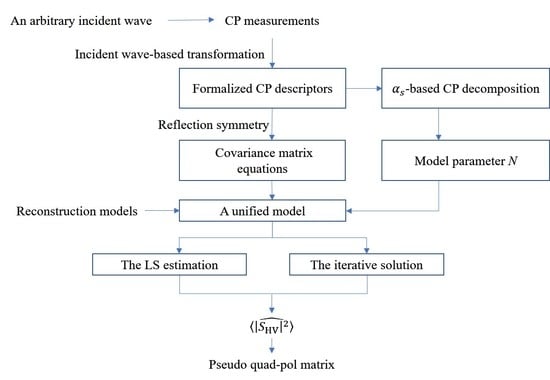
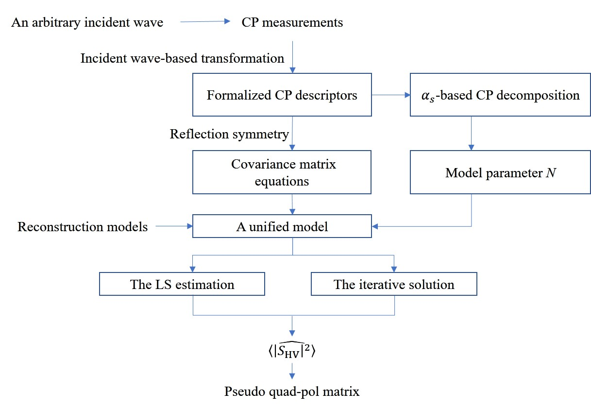
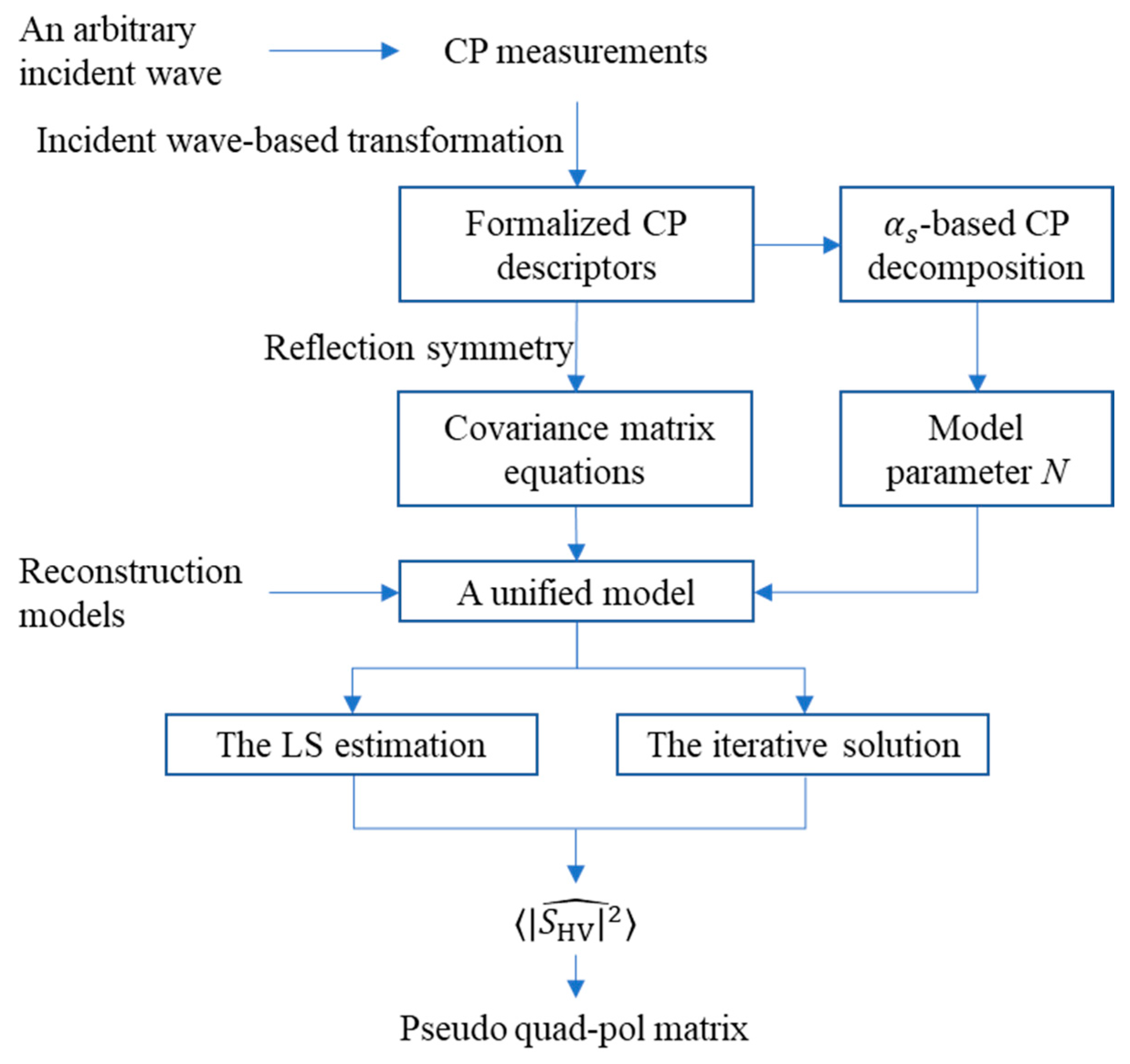
An overview of the current related techniques is presented. The current iteration-based techniques, which were developed for either the circular or the linear CP modes, are also extended for the general CP mode. The contents of this study are summarized in Figure 1. In Section 2, we introduce the test data used for illustration. In Section 3, the formalism of the general CP descriptors in terms of the covariance matrix is introduced. In Section 4, we first summarize the reconstruction models, and then based on the formalized CP covariance matrix the iterative solving approach is extended for the general CP SAR images. In Section 5, the LS model function is proposed, and the approximation to the model parameter $N$ is also given. In Section 6, multiple polarimetric data sets are used to show the reconstruction performances of both the iterative and the LS methods, as well as the abilities of different CP modes for revealing the quad-pol information. Finally, the paper is summarized in Section 7.

2. Test Data

RADARSAT-2 data acquired over Fuzhou, China, and Wallerfing, Germany, as well as ALOS-2/PALSAR data acquired over San Francisco are used for verification. Corresponding Pauli-basis images are shown in Figure 2. The Fuzhou area has complex terrain types, including dispersed residential areas, mountain and hills, agriculture fields, wetlands, and sea surface. The Fuzhou data set was collected on 20 October 2013, with incidence angle ranging from 34.4° to 36.0°. This image has 6140 × 3332 pixels, and the pixel spacing is 4.73 × 4.81 m². The Wallerfing area consists of large agriculture fields. Data sets were collected regularly over this area to monitor the crop growth in 2014. The data sets acquired on 28 May, 21 June, 15 July, and 8 August 2014 are included for demonstration. All the Wallerfing data sets were collected with incidence angle ranging from 40.2° to 41.6° on the descending pass. The image has 2001 × 2001 pixels, and the pixel spacing is 4.73 × 5.12 m². The farmland mainly consists of 5 crop types, i.e., barley, corn, potato, sugarbeat, and wheat. The ground truth of crop types is also given in Figure 2. The San Francisco data was collected on 21 August 2018 with the center incidence angle of 33.871°. The image has 2389 × 2640 pixels, and the pixel spacing is 2.8 × 3.2 m². The transversal lines and the outlined areas in Figure 2c,d will be used for analysis in experiments.

3. Formalism of the CP Descriptors

In this section, we will briefly introduce the formalized scattering vector and covariance matrix [18].

A general form of the electromagnetic field is represented by a transverse ellipse which is described by two parameters, i.e., the ellipse orientation angle $\theta$ and the ellipticity angle $\chi$ [1], as follows.

$$\begin{array}{cc}{\stackrel{\rightharpoonup }{E}}_i\left(\begin{array}{cc}\theta ,& \chi \end{array}\right)& =\left[\begin{array}{c}{E}_{ix}\left(\begin{array}{cc}\theta ,& \chi \end{array}\right)\\ E_{iy}\left(\begin{array}{cc}\theta ,& \chi \end{array}\right)\end{array}\right]=\left[\begin{array}{cc}cos\theta & -sin\theta \\ sin\theta & cos\theta \end{array}\right]\left[\begin{array}{c}cos\chi \\ jsin\chi \end{array}\right]\hfill \\ & =\left[\begin{array}{c}cos\theta cos\chi -jsin\theta sin\chi \\ sin\theta cos\chi +jcos\theta sin\chi \end{array}\right]\hfill \end{array}$$

(1)

where $\left|\right|{\stackrel{\rightharpoonup }{E}}_i\left(\begin{array}{cc}\theta ,& \chi \end{array}\right)\left|\right|=1$. The CP system measures a projection of the complex scattering matrix $\mathit{S}$ onto a transmitted wave. Then for an arbitrary transmit wave ${\stackrel{\rightharpoonup }{E}}_i\left(\begin{array}{cc}\theta ,& \chi \end{array}\right)$, the received backscattered wave ${\stackrel{\rightharpoonup }{E}}_r\left(\begin{array}{cc}\theta ,& \chi \end{array}\right)$ is

$$\begin{array}{cc}{\stackrel{\rightharpoonup }{E}}_r\left(\begin{array}{cc}\theta ,& \chi \end{array}\right)=\left[\begin{array}{c}{E}_{HC}\left(\begin{array}{cc}\theta ,& \chi \end{array}\right)\\ E_{VC}\left(\begin{array}{cc}\theta ,& \chi \end{array}\right)\end{array}\right]& =\mathit{S}{\stackrel{\rightharpoonup }{E}}_i\left(\begin{array}{cc}\theta ,& \chi \end{array}\right)=\left[\begin{array}{cc}{S}_{HH}& S_{HV}\\ S_{VH}& S_{VV}\end{array}\right]\left[\begin{array}{c}{E}_{ix}\left(\begin{array}{cc}\theta ,& \chi \end{array}\right)\\ E_{iy}\left(\begin{array}{cc}\theta ,& \chi \end{array}\right)\end{array}\right]\hfill \\ & =\left[\begin{array}{c}{E}_{ix}\left(\begin{array}{cc}\theta ,& \chi \end{array}\right)S_{HH}+E_{iy}\left(\begin{array}{cc}\theta ,& \chi \end{array}\right)S_{HV}\\ E_{iy}\left(\begin{array}{cc}\theta ,& \chi \end{array}\right)S_{VV}+E_{ix}\left(\begin{array}{cc}\theta ,& \chi \end{array}\right)S_{VH}\end{array}\right]\hfill \end{array}$$

(2)

For an arbitrary $\mathit{S}$, the received compact (or traditional dual) polarimetric signal is totally dependent on $\theta$ and $\chi$. For the commonly considered linear π/4, left circular, right circular, horizontal and vertical transmitted waves, the values of $\left(\begin{array}{cc}\theta ,& \chi \end{array}\right)$ are $\left(\begin{array}{cc}\mathsf{\pi }/4,& 0\end{array}\right)$, $\left(\left[\begin{array}{cc}-\mathsf{\pi }/2& \mathsf{\pi }/2\end{array}\right]\begin{array}{cc},& \mathsf{\pi }/4\end{array}\right)$, $\left(\left[\begin{array}{cc}-\mathsf{\pi }/2& \mathsf{\pi }/2\end{array}\right]\begin{array}{cc},& -\mathsf{\pi }/4\end{array}\right)$, $\left(\begin{array}{cc}0,& 0\end{array}\right)$ and $\left(\begin{array}{cc}\mathsf{\pi }/2,& 0\end{array}\right)$, respectively. Note that the circular polarization is not affected by wave orientation angles, and thus $\theta \in \left[\begin{array}{cc}-\mathsf{\pi }/2& \mathsf{\pi }/2\end{array}\right]$. ${\stackrel{\rightharpoonup }{E}}_r\left(\begin{array}{cc}\theta ,& \chi \end{array}\right)$ in (2) is received in the linear-polarization orthogonal basis and can be easily transformed to the circular polarization basis through a unitary transformation [1,6,21]. The dual-polarization measurement is independent of the elliptical basis of radar receivers, and thus we only discuss the linear H/V-polarization received CP data. We notice that $E_{\mathrm{HC}}$ contains $S_{\mathrm{HH}}$ and $E_{\mathrm{VC}}$ contains $S_{\mathrm{VV}}$ when none of $E_{ix}\left(\begin{array}{cc}\theta ,& \chi \end{array}\right)$ and $E_{iy}\left(\begin{array}{cc}\theta ,& \chi \end{array}\right)$ is 0. Then, the scattering vector (2) can be formulated as

$${\stackrel{\rightharpoonup }{k}}_1=\left[\begin{array}{c}{E}_1\\ E_2\end{array}\right]={\left(diag\left({\stackrel{\rightharpoonup }{E}}_i\left(\begin{array}{cc}\theta ,& \chi \end{array}\right)\right)\right)}^{-1}{\stackrel{\rightharpoonup }{E}}_r\left(\begin{array}{cc}\theta ,& \chi \end{array}\right)=\left[\begin{array}{c}\frac{E_{HC}\left(\begin{array}{cc}\theta ,& \chi \end{array}\right)}{E_{ix}\left(\begin{array}{cc}\theta ,& \chi \end{array}\right)}\\ \frac{E_{VC}\left(\begin{array}{cc}\theta ,& \chi \end{array}\right)}{E_{iy}\left(\begin{array}{cc}\theta ,& \chi \end{array}\right)}\end{array}\right]=\left[\begin{array}{c}{S}_{HH}+x{S}_{HV}\\ S_{VV}+y{S}_{VH}\end{array}\right]$$

(3)

where $\mathrm{diag}\left(·\right)$ is the diagonal matrix of a vector, and

$$x=\frac{E_{iy}\left(\begin{array}{cc}\theta ,& \chi \end{array}\right)}{E_{ix}\left(\begin{array}{cc}\theta ,& \chi \end{array}\right)}, y=\frac{E_{ix}\left(\begin{array}{cc}\theta ,& \chi \end{array}\right)}{E_{iy}\left(\begin{array}{cc}\theta ,& \chi \end{array}\right)}$$

are the wave component ratios. $E_1$ and $E_2$ are the formalized elements for ${\stackrel{\rightharpoonup }{E}}_r\left(\begin{array}{cc}\theta ,& \chi \end{array}\right)$ to characterize the scattered wave. This formalism is only for the general compact polarimetric mode. It is not applicable to the conventional dual polarizations, i.e., the $S_{\mathrm{HV}}/S_{\mathrm{VV}}$ or $S_{\mathrm{HH}}/S_{\mathrm{VH}}$ measurements.

From the defined scattering vector ${\stackrel{\rightharpoonup }{k}}_1$, the second order product, named as the CP covariance matrix following that in full polarimetry, is constructed for the partially polarized backscattered waves, as follows.

$${\mathit{C}}_2=\langle {\stackrel{\rightharpoonup }{k}}_1{\stackrel{\rightharpoonup }{k}}_1^H\rangle =\left[\begin{array}{cc}{\langle \left|E_1\right|}^2\rangle & \langle E_1{E}_2{}^{*}\rangle \\ \langle E_2{E}_1{}^{*}\rangle & \langle {\left|E_2\right|}^2\rangle \end{array}\right]$$

(4)

where ^H denotes matrix conjugate transpose, and $\langle ·\rangle$ denotes ensemble average. ${\mathit{C}}_2$ is the basis in this study to analyze the general CP matrix for the multi-polarization reconstruction.

The formalized scattering vector in (3) and the corresponding CP covariance matrix defined in (4) provide a unified method representing CP data. For a monostatic polarimetric SAR and reciprocal scatterers, the scattering matrix is symmetric, i.e., $S_{\mathrm{HV}}=S_{\mathrm{VH}}$. In this case, expansion of ${\mathit{C}}_2$ in terms of the scattering coefficients of the medium is given in (5). If scattering reflection symmetry is further assumed for the CP covariance matrix, which means the components involving products of co-polarized and cross-polarized terms are much smaller than the others and thus negligible, ${\mathit{C}}_2$ only contains the co-polarized and cross-polarized terms, as shown in (6). When the transmit wave is linearly polarized, e.g., in the linear π/4 mode, ${\mathit{C}}_2$ has the same form as the wave covariance matrix [7,8,12] except that the matrix power is doubled. When the transmit wave is circularly polarized, ${\mathit{C}}_2$ has a different form from the wave covariance matrix as that shown in (4) in [8]. This formalism provides a unified description for the backscattered wave, which facilitates the analysis of CP imagery. Under this formalism, the system of non-linear equations for the reconstruction is easily formulated as a function of the transmit wave, which will be discussed in Section 4 and Section 5.

$$\begin{array}{cc}{\mathit{C}}_2=\left[\begin{array}{cc}\langle C_{11}\rangle & \langle C_{12}\rangle \\ \langle C_{12}{}^{*}\rangle & \langle C_{22}\rangle \end{array}\right]& =\left[\begin{array}{cc}\langle {\left|S_{HH}\right|}^2\rangle & \langle S_{HH}{S}_{VV}^{*}\rangle \\ \langle S_{VV}{S}_{HH}^{*}\rangle & \langle {\left|S_{VV}\right|}^2\rangle \end{array}\right]+\langle {\left|S_{HV}\right|}^2\rangle \left[\begin{array}{cc}{\left|x\right|}^2& x{y}^{*}\\ x^{*}y& {\left|y\right|}^2\end{array}\right]\hfill \\ & +\left[\begin{array}{cc}2Re\left(x^{*}\langle S_{HH}{S}_{HV}^{*}\rangle \right)& x\langle S_{HV}{S}_{VV}^{*}\rangle +y^{*}\langle S_{HH}{S}_{HV}^{*}\rangle \\ x^{*}\langle S_{VV}{S}_{HV}^{*}\rangle +y\langle S_{HV}{S}_{HH}^{*}\rangle & 2Re\left(y^{*}\langle S_{VV}{S}_{HV}^{*}\rangle \right)\end{array}\right]\hfill \end{array}$$

(5)

$${\mathit{C}}_2=\left[\begin{array}{cc}\langle C_{11}\rangle & \langle C_{12}\rangle \\ \langle C_{12}{}^{*}\rangle & \langle C_{22}\rangle \end{array}\right]=\left[\begin{array}{cc}\langle {\left|S_{HH}\right|}^2\rangle & \langle S_{HH}{S}_{VV}^{*}\rangle \\ \langle S_{VV}{S}_{HH}^{*}\rangle & \langle {\left|S_{VV}\right|}^2\rangle \end{array}\right]+\langle {\left|S_{HV}\right|}^2\rangle \left[\begin{array}{cc}{\left|x\right|}^2& x{y}^{*}\\ x^{*}y& {\left|y\right|}^2\end{array}\right]$$

(6)

4. Pseudo Quad-Pol Image Reconstruction Model and the Iterative Approach

4.1. A General Form of Reconstruction Models

In the literature, there are mainly five reconstruction models. The reconstruction models in [7,8,9,10,11] have the same form as follows.

$$\frac{\langle {\left|S_{\mathrm{HV}}\right|}^2\rangle }{\langle {\left|S_{\mathrm{HH}}\right|}^2\rangle +\langle {\left|S_{\mathrm{VV}}\right|}^2\rangle }=\frac{1-\left|\rho \right|}{N}$$

(7)

where $\rho$ is the co-polarized correlation defined by

$$\rho =\frac{\langle S_{\mathrm{HH}}{S}_{\mathrm{VV}}^{*}\rangle }{\sqrt{\langle {\left|S_{\mathrm{HH}}\right|}^2\rangle \langle {\left|S_{\mathrm{VV}}\right|}^2\rangle }}$$

(8)

and $N$ is the model parameter derived from either theoretical analysis or empirical curve fitting. The Souyris et al. model [7] is derived from a pseudo-deterministic relationship by linking $\rho$ and the cross- and co-polarization ratio. By assuming the backscattered signal is either fully polarized or fully depolarized, $N$ is obtained as 4. The Nord et al. model [8] is approximated from a mathematical inequality, and the equality is asserted by a relatively small difference of the two sides of the inequality. Both Collins’s [9,10] and Li’s [11] models are empirical models but with different regression equations, where Collins et al. used the exponential model to fit $N$ by considering the incidence angle, and Li et al. fitted $N$ as a function of the polarization ratio.

A backscattered process is a mixture of several elemental scattering processes. By assuming that the backscattered energy is a sum of the surface scattering power $P_{\mathrm{s}}$, double-bounce scattering power $P_{\mathrm{d}}$, and volume scattering power $P_{\mathrm{v}}$, we established a decomposition-based power-weighted reconstruction model [12], as shown in (9), which use $\mathrm{Re}(\langle S_{\mathrm{HH}}{S}_{\mathrm{VV}}^{*}\rangle )$ as an indicator to discriminate between the surface and double-bounce reflections (refer to [12] for more details).

$$\frac{\langle {\left|S_{\mathrm{HV}}\right|}^2\rangle }{\langle {\left|S_{\mathrm{HH}}\right|}^2\rangle +\langle {\left|S_{\mathrm{VV}}\right|}^2\rangle }=\frac{1-\mathrm{sg}\left|\rho \right|}{N}$$

(9)

where $\mathrm{sg}=\mathrm{sign}\left(\mathrm{Re}(\langle S_{\mathrm{HH}}{S}_{\mathrm{VV}}^{*}\rangle )\right)$ is a signum function, and N = 4(2P_d + P_v)/P_v). This power-weighted reconstruction model has an extra parameter $\mathrm{sg}$ which is either 1 or −1. In the following sections, we use (9) as a general formulation of the reconstruction models, and the model parameters are summarized in

Table 1. Parameters of the reconstruction models.

Souyris et al. [7]	Nord et al. [8]	Collins et al. [9]	Li et al. [11]	Yin et al. [12]
sg = 1	sg = 1	sg = 1	sg = 1	$\mathrm{sg}=\mathrm{sign}\left(\mathrm{Re}\left(\langle S_{\mathrm{HH}}{S}_{\mathrm{VV}}^{*}\rangle \right)\right)$
N = 4	$N=\frac{\langle {\left|S_{\mathrm{HH}}-S_{\mathrm{VV}}\right|}^2\rangle }{\langle {\left|S_{\mathrm{HV}}\right|}^2\rangle }$	Empirical N	Empirical N	$N=4\frac{2P_{\mathrm{d}}+P_{\mathrm{v}}}{P_{\mathrm{v}}}$

. The model parameter $N$ is updated during the iterative reconstruction procedure in the studies [8,11,12], which are referred to as the variable $N$ methods. While parameter $N$ is a constant in the methods [7,9], which are referred to as the constant $N$ methods.

4.2. Unified Experssion of the Model Parameters

In previous studies, the reason that different CP modes need different reconstruction procedures arises from the fact that different equations are necessary to calculate the co-polarized correlation coefficient $\rho$. See Equations (7) and (11) in [8] for instance. However, with the unified CP covariance matrix defined in (6), the co-polarized coherence has a general expression, given by

$$\rho =\frac{\langle C_{12}\rangle -\langle {\left|S_{\mathrm{HV}}\right|}^2\rangle x{y}^{*}}{\sqrt{\left(\langle C_{11}\rangle -\langle {\left|S_{\mathrm{HV}}\right|}^2\rangle {\left|x\right|}^2\right)\left(\langle C_{22}\rangle -\langle {\left|S_{\mathrm{HV}}\right|}^2\rangle {\left|y\right|}^2\right)}}$$

(10)

$x$ and $y$ are parameters depending on the transmit wave. With this expression, the reconstruction model in (9) is applicable to all CP modes.

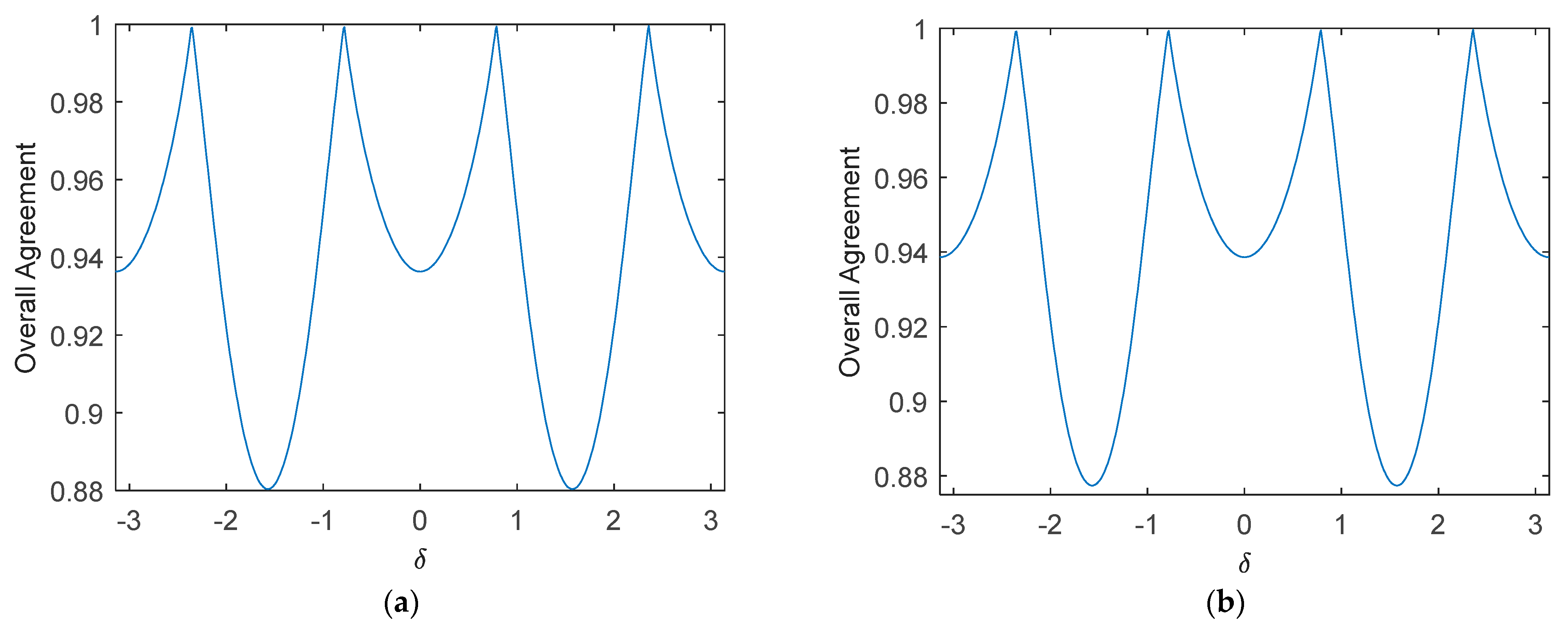
Next, we consider the parameter $\mathrm{sg}$, which only exists in the decomposition-based reconstruction model [12]. Our previous studies [12,14] tested that for the linear π/4 mode, the total agreement between $\mathrm{sign}\left(\mathrm{Re}(\langle C_{12}\rangle \right))$ and $\mathrm{sign}\left(\mathrm{Re}(\langle S_{\mathrm{HH}}{S}_{\mathrm{VV}}^{*}\rangle )\right)$ is quite good. For the general case, from the off-diagonal term of (6) it is observed that $\langle C_{12}\rangle =\langle S_{\mathrm{HH}}{S}_{\mathrm{VV}}^{*}\rangle +\langle {\left|S_{\mathrm{HV}}\right|}^2\rangle x{y}^{*}$, which indicates the sign of $\langle S_{\mathrm{HH}}{S}_{\mathrm{VV}}^{*}\rangle$ is only affected by $\langle {\left|S_{\mathrm{HV}}\right|}^2\rangle e^{j2\delta }$, where $\delta =\mathrm{angle}\left(E_{iy}{E}_{ix}^{*}\right)$ is the relative phase of the transmit wave, which is a known number. For the area dominated by a single scattering mechanism, $\left|\mathrm{Re}(\langle S_{\mathrm{HH}}{S}_{\mathrm{VV}}^{*}\rangle )\right|$ is usually larger than $\langle {\left|S_{\mathrm{HV}}\right|}^2\rangle$. Therefore, for the general reconstruction algorithm, we still use $\mathrm{Re}(\langle C_{12}\rangle )$to approximate the decision whether backscatter is dominated by surface or double-bounce scattering [12,13,14]. Let ${\mathrm{sg}}_c=\mathrm{sign}\left(\mathrm{Re}(\langle C_{12}\rangle )\right)$. By using the test data shown in Section 2, variation of the total agreement between $\mathrm{sign}\left(\mathrm{Re}(\langle C_{12}\rangle \right))$ and $\mathrm{sign}\left(\mathrm{Re}(\langle S_{\mathrm{HH}}{S}_{\mathrm{VV}}^{*}\rangle )\right)$ with the transmit wave parameter $\delta$ is shown in Figure 3. It shows that for the C-band data when the relative phase $\delta$ is ±π/4 or ±3π/4, the total agreement is as high as 99.92% (99.96% for the L-band data), and when the relative phase $\delta$ is ±π/2 (e.g., one possible mode is the circular modes), the total agreement is lowest but still with a good percentage of 88%. Areas dominated by double-bounce scattering or double-bounce scattering taking a relatively high amount, such as the urban areas, would have a lower overall agreement. When the transmit wave is linearly polarized (i.e., $\delta =0$ or ±π), the overall agreement is 93.65% for C-band data and 93.83% for L-band data. The general form of the reconstruction models with model parameters derived from (6) constructs the unified reconstruction model.

4.3. The Decomposition-Based Variable N

The three-component model-based decomposition [16] is written as

$$\mathit{C}=f_{\mathrm{s}}\left[{\mathit{C}}_{\mathrm{s}}\right]+f_{\mathrm{d}}\left[{\mathit{C}}_{\mathrm{d}}\right]+f_{\mathrm{v}}\left[{\mathit{C}}_{\mathrm{v}}\right]$$

(11)

where $\mathit{C}=\langle {\stackrel{\rightharpoonup }{k}}_L{\stackrel{\rightharpoonup }{k}}_L^{\mathrm{H}}\rangle$ is the fully polarimetric covariance matrix with ${\stackrel{\rightharpoonup }{k}}_L={\left[\begin{array}{ccc}{S}_{\mathrm{HH}}& \sqrt{2}{S}_{\mathrm{HV}}& S_{\mathrm{VV}}\end{array}\right]}^{\mathrm{T}}$; $f_{\mathrm{s}}$, $f_{\mathrm{d}}$ and $f_{\mathrm{v}}$ are the decomposed parameters to be determined corresponding to the surface, double-bounce, and volume scattering models, which are given by

$$\left[{\mathit{C}}_{\mathrm{s}}\right]=\left[\begin{array}{ccc}{\left|\beta \right|}^2& 0& \beta \\ 0& 0& 0\\ {\beta }^{*}& 0& 1\end{array}\right],\left[{\mathit{C}}_{\mathrm{d}}\right]=\left[\begin{array}{ccc}{\left|\alpha \right|}^2& 0& \alpha \\ 0& 0& 0\\ {\alpha }^{*}& 0& 1\end{array}\right],\left[{\mathit{C}}_{\mathrm{v}}\right]=\left[\begin{array}{ccc}1& 0& b\\ 0& 1-b& 0\\ b^{*}& 0& 1\end{array}\right], b\in \left[\begin{array}{cc}0,& 1\end{array}\right]$$

(12)

where $\beta$ and $\alpha$ are model parameters with $\arg \left(\beta \right)\approx 0$ for surface scattering and $\arg \left(\alpha \right)\approx \pm \mathsf{\pi }$ for double-bounce scattering. In Freeman and Durden’s 3-component decomposition, $b$ is set to $1/3$. However, for the purpose of the pseudo quad-pol image reconstruction, we set $b=0$ [12,14]. According to the general CP expression in (6), scattering models in (12) are synthesized as follows.

$${\left[{\mathit{C}}_{\mathrm{s}}\right]}_{\mathrm{CP}}=\left[\begin{array}{cc}{\left|\beta \right|}^2& \beta \\ {\beta }^{*}& 1\end{array}\right],{\left[{\mathit{C}}_{\mathrm{d}}\right]}_{\mathrm{CP}}=\left[\begin{array}{cc}{\left|\alpha \right|}^2& \alpha \\ {\alpha }^{*}& 1\end{array}\right],{\left[{\mathit{C}}_{\mathrm{v}}\right]}_{\mathrm{CP}}=\left[\begin{array}{cc}1+0.5{\left|x\right|}^2& 0.5x{y}^{*}\\ 0.5x^{*}y& 1+0.5{\left|y\right|}^2\end{array}\right]$$

(13)

Then the general CP covariance matrix can be expanded as

$${\mathit{C}}_2=f_{\mathrm{sc}}{\left[{\mathit{C}}_{\mathrm{s}}\right]}_{\mathrm{CP}}+f_{\mathrm{dc}}{\left[{\mathit{C}}_{\mathrm{d}}\right]}_{\mathrm{CP}}+f_{\mathrm{vc}}{\left[{\mathit{C}}_{\mathrm{v}}\right]}_{\mathrm{CP}}$$

(14)

where $f_{\mathrm{sc}}$, $f_{\mathrm{dc}}$, and $f_{\mathrm{vc}}$ are expansion coefficients. This decomposition should be performed under the constraint that the ratio of the total backscattered powers of the FP and the CP data is known. Otherwise, the CP decomposed powers cannot be related to the FP decomposed powers. Only when ${\left|x\right|}^2={\left|y\right|}^2$, which corresponds to the CP modes with either $\theta =\pm \mathsf{\pi }/4$ or $\chi =\pm \mathsf{\pi }/4$, the decomposed powers can be expressed as a function of $\langle {\left|S_{\mathrm{HV}}\right|}^2\rangle$. In this case, the total powers of the FP covariance matrix and the formalized CP covariance matrix are equal by assuming reflection symmetry.

We assume that the CP decomposed volume scattering power is equal to that of FP, i.e., $f_{\mathrm{vc}}=f_{\mathrm{v}}=2\langle {\left|S_{\mathrm{HV}}\right|}^2\rangle$ (refer to (3) in [14]). Then, (14) can be solved following the Freeman and Durden procedure. When $\mathrm{Re}(\langle C_{12}\rangle )$ is positive, surface scattering is dominant and we let $\alpha =-1$. When $\mathrm{Re}(\langle C_{12}\rangle )$ is negative, double-bounce scattering is dominant and we let $\beta =1$. It is easily derived that the decomposed powers, represented as a function of $\langle {\left|S_{\mathrm{HV}}\right|}^2\rangle$, are

$$\{\begin{array}{c}\begin{array}{cc}if \mathrm{Re}\left(\langle C_{12}\rangle \right)>0& then\alpha =-1\end{array}\\ P_{\mathrm{dc}}=2\frac{XY-{\left|Z\right|}^2}{X+Y+2Re\left(Z\right)}\\ P_{\mathrm{vc}}=3f_{\mathrm{vc}}=6\langle {\left|S_{\mathrm{HV}}\right|}^2\rangle \\ P_{\mathrm{sc}}=spa{n}_{\mathrm{c}}-P_{\mathrm{dc}}-P_{\mathrm{vc}}\end{array}\begin{array}{cc}or& \{\begin{array}{c}\begin{array}{cc}if \mathrm{Re}\left(\langle C_{12}\rangle \right)<0& then\beta =1\end{array}\\ P_{\mathrm{sc}}=2\frac{XY-{\left|Z\right|}^2}{X+Y-2Re\left(Z\right)}\\ P_{\mathrm{vc}}=3f_{\mathrm{vc}}=6\langle {\left|S_{\mathrm{HV}}\right|}^2\rangle \\ P_{\mathrm{dc}}=spa{n}_{\mathrm{c}}-P_{\mathrm{sc}}-P_{\mathrm{vc}}\end{array}\end{array}$$

(15)

where

$$\{\begin{array}{c}X=\langle C_{11}\rangle -3\langle {\left|S_{\mathrm{HV}}\right|}^2\rangle \\ Y=\langle C_{22}\rangle -3\langle {\left|S_{\mathrm{HV}}\right|}^2\rangle \\ Z=\langle C_{12}\rangle -\langle {\left|S_{\mathrm{HV}}\right|}^2\rangle x{y}^{*}\end{array}$$

$spa{n}_{\mathrm{c}}=\langle C_{11}\rangle +\langle C_{22}\rangle$. $P_{\mathrm{sc}}$, $P_{\mathrm{dc}}$, and $P_{\mathrm{vc}}$ are the surface, double-bounce, and volume scattering powers of CP data, respectively. Note that this solution is only valid for the case when ${\left|x\right|}^2={\left|y\right|}^2$, i.e., $\left|x\right|=\left|y\right|=1$. Then $N$ can be updated by (16), which is embedded in the iteration procedure.

$$N=4\left(2P_{\mathrm{dc}}+P_{\mathrm{vc}}\right)/P_{\mathrm{vc}}$$

(16)

4.4. The Iterative Solving Approach

By assuming reflection symmetry, we can obtain 3 equations from (6) for each pixel. However, we have four unknows, i.e., $\langle {\left|S_{\mathrm{HH}}\right|}^2\rangle$, $\langle {\left|S_{\mathrm{VV}}\right|}^2\rangle$, $\langle {\left|S_{\mathrm{HV}}\right|}^2\rangle$, and $\langle S_{\mathrm{HH}}{S}_{\mathrm{VV}}^{*}\rangle$. When the reconstruction model is further considered as the fourth equation, $\langle {\left|S_{\mathrm{HV}}\right|}^2\rangle$ can be solved by an iterative approach, as the procedures introduced in [7,8,9,10,11,12,13]. These studies were only discussed for the typical linear- or circular- transmit CP mode.

Based on the unified CP descriptor and the reconstruction model in (9), the iterative approach for solving $\langle {\left|S_{\mathrm{HV}}\right|}^2\rangle$ for the mode with $\left|x\right|=\left|y\right|$ is summarized as below.

Step 0: Initialization

$$\begin{gathered} {\rho }_{\left(0\right)}=\frac{\langle C_{12}\rangle }{\sqrt{\langle C_{11}\rangle \langle C_{22}\rangle }} \\ \langle {\left|S_{\mathrm{HV}}\right|}^2\rangle {}_{\left(0\right)}=\left(\langle C_{11}\rangle +\langle C_{22}\rangle \right) \times \frac{1-{\mathrm{sg}}_c\left|{\rho }_{\left(0\right)}\right|}{N_{\left(0\right)}+\left({\left|x\right|}^2+{\left|y\right|}^2\right)\left(1-{\mathrm{sg}}_c\left|{\rho }_{\left(0\right)}\right|\right)} \end{gathered}$$

(17)

Step 1: Iteration

$$\begin{array}{cc}\hfill {\rho }_{\left(i+1\right)}& =\frac{\langle C_{12}\rangle -\langle {\left|S_{\mathrm{HV}}\right|}^2\rangle {}_{\left(i\right)}x{y}^{*}}{\sqrt{\left(\langle C_{11}\rangle -\langle {\left|S_{\mathrm{HV}}\right|}^2\rangle {}_{\left(i\right)}{\left|x\right|}^2\right)\left(\langle C_{22}\rangle -\langle {\left|S_{\mathrm{HV}}\right|}^2\rangle {}_{\left(i\right)}{\left|y\right|}^2\right)}}\hfill \\ \hfill \langle {\left|S_{\mathrm{HV}}\right|}^2\rangle {}_{\left(i+1\right)}& =\left(\langle C_{11}\rangle +\langle C_{22}\rangle \right) \times \frac{1-{\mathrm{sg}}_c\left|{\rho }_{\left(i+1\right)}\right|}{N_{\left(i+1\right)}+\left({\left|x\right|}^2+{\left|y\right|}^2\right)\left(1-{\mathrm{sg}}_c\left|{\rho }_{\left(i+1\right)}\right|\right)}\hfill \end{array}$$

(18)

where $i=0, 1, 2\cdots$is the iteration number. For the methods in [7,8,9,10,11], ${\mathrm{sg}}_c=\mathrm{sg}=1$, as listed in Table 1. For the decomposition-based reconstruction model [12], ${\mathrm{sg}}_c=\mathrm{sign}\left(\mathrm{Re}\left(\langle C_{12}\rangle \right)\right)$. $N$ varies and updated according to different models. For the Nord et al. [8] and the Li et al. [11] models, $N$ can be updated easily through the constructed FP covariance matrix at each iteration. For the decomposition-based method in [12], the model parameter $N$ is updated by the three-component decomposed-powers, which are a function of the cross-pol term $\langle {\left|S_{\mathrm{HV}}\right|}^2\rangle {}_{\left(i\right)}$. The updating method has been introduced in Section 4.3. Given an estimated value for $\langle {\left|S_{\mathrm{HV}}\right|}^2\rangle {}_c$, the pseudo quad-pol data is constructed as

$${\mathit{C}}_{\mathrm{pseudo}-\mathrm{quad}}=\left[\begin{array}{ccc}\langle C_{11}\rangle -\langle {\left|S_{\mathrm{HV}}\right|}^2\rangle {}_c{\left|x\right|}^2& 0& \langle C_{12}\rangle -\langle {\left|S_{\mathrm{HV}}\right|}^2\rangle {}_{c}x{y}^{*}\\ 0& 2\langle {\left|S_{\mathrm{HV}}\right|}^2\rangle {}_c& 0\\ \langle C_{12}^{*}\rangle -\langle {\left|S_{\mathrm{HV}}\right|}^2\rangle {}_c{x}^{*}y& 0& \langle C_{22}\rangle -\langle {\left|S_{\mathrm{HV}}\right|}^2\rangle {}_c{\left|y\right|}^2\end{array}\right]$$

(19)

The iteration usually converges after several steps. However, the estimated cross-polarized term is often overestimated [7,8,9,14]. In the next section, we propose a least squares error estimation framework to optimize $\langle {\left|S_{\mathrm{HV}}\right|}^2\rangle$ for all CP modes.

5. Pseudo Quad-Pol Image Reconstruction by Using the Least Squares Estimation

5.1. Least Squares Objective Function

The LS estimation is performed in a local window, and can be applied to both multi-look and single-look data. However, if the multi-look data is used for the LS estimation, the reconstructed pseudo quad-pol image may be over-filtered. Therefore, we use the single-look complex data to fit the reconstruction model. Assuming that an optimal cross-polarized term $\langle {\left|S_{\mathrm{HV}}\right|}^2\rangle$ exists, then for each pixel in the window, the system of non-linear equations is

$$\begin{array}{c}{\left|S_{\mathrm{HH}}\right|}^2=C_{11}-\langle {\left|S_{\mathrm{HV}}\right|}^2\rangle {\left|x\right|}^2\\ {\left|S_{\mathrm{VV}}\right|}^2=C_{22}-\langle {\left|S_{\mathrm{HV}}\right|}^2\rangle {\left|y\right|}^2\\ S_{\mathrm{HH}}{S}_{\mathrm{VV}}^{*}=C_{12}-\langle {\left|S_{\mathrm{HV}}\right|}^2\rangle x{y}^{*}\\ \frac{\langle {\left|S_{\mathrm{HV}}\right|}^2\rangle }{{\left|S_{\mathrm{HH}}\right|}^2+{\left|S_{\mathrm{VV}}\right|}^2}=\frac{1-{\mathrm{sg}}_c\left|\rho \right|}{N}\end{array}$$

(20)

where $\rho$ is the local co-polarized correlation coefficient, as defined in (10). Substituting the first 3 equations in (20) to the last one, a least squares error objective function is obtained for $\langle {\left|S_{\mathrm{HV}}\right|}^2\rangle$, as follows.

$$\langle {\left|S_{\mathrm{HV}}\right|}^2\rangle {}_c=\underset{\langle {\left|S_{\mathrm{HV}}\right|}^2\rangle }{\mathrm{argmin}}{\displaystyle \sum }_{i=1}^n{\left(\langle {\left|S_{\mathrm{HV}}\right|}^2\rangle N-\left(spa{n}_{c\left(i\right)}-\langle {\left|S_{\mathrm{HV}}\right|}^2\rangle \left({\left|x\right|}^2+{\left|y\right|}^2\right)\right)\left(1-{\mathrm{sg}}_c\left|\rho \right|\right)\right)}^2$$

(21)

where i is the i-th pixel in the local window, $n$ is the window pixel number, and $\langle {\left|S_{\mathrm{HV}}\right|}^2\rangle {}_c$ is the LS estimate for the problem. The local window can be either square or non-square, if an edge-aligned non-square window as that in [22] is used, image texture information will be better preserved. The LS solution $\langle {\left|S_{\mathrm{HV}}\right|}^2\rangle {}_c$ is for the center pixel of the window. After optimization, the reconstructed FP covariance matrix is obtained by (19).

In the LS model function, since pixels in a local window are used to find the best fitting parameter, $N$ should also be an average estimate from the local window. In this study, we do not consider the empirical models, because they are related to specific observation scenarios. The variable $N$ method is not applicable to the LS estimation because $N$ needs to be a fixed number. The Souyris et al. model [7] can be integrated into the LS objective function since the model parameters are constant, with parameter settings as ${\mathrm{sg}}_c=1$ and $N=4$. For the decomposition-based model, ${\mathrm{sg}}_c=\mathrm{sign}\left(\mathrm{Re}(\langle C_{12}\rangle )\right)$ and $N=4\left(2P_{\mathrm{dc}}+P_{\mathrm{vc}}\right)/P_{\mathrm{vc}}$, where $P_{\mathrm{dc}}$ and $P_{\mathrm{vc}}$ are the decomposed powers from the CP data. In [14], we proposed a new method to give a priori estimate for $N$ based on the linear π/4 mode. In [19], the decomposition was extended to a general case. Therefore, in this paper, the decomposed powers are used to estimate $N$.

5.2. The Decomposition-Based Approximation to the Constant N

$N$ is a parameter indicating the ratio between double-bounce and volume scattering components. The iterative approach updates $N$ based on the intermediate result of $\langle {\left|S_{\mathrm{HV}}\right|}^2\rangle$. For the LS estimation, $N$ should be a constant. In [20], a CP decomposition was proposed for the circular CP mode, where the single scattering mechanism is modeled by the symmetric scattering type angle ${\alpha }_s$. In [19], we generalize this decomposition to the general CP case, but leave one degree of freedom, i.e., $F_p$ in (14) in [19], for the volume scattering model, and take it as an argument for the decomposed powers. In this study, when approximating $N$, let $F_p=1$. The reasons are as follows. (1) The decomposition-based reconstruction model was proposed with $F_p=1$ [12]. (2) The volume scattering model has the same degree of polarization of $1/3$ for all the CP modes which are with balanced transmit wave channel amplitudes (i.e., $\left|E_{ix}\right|=\left|E_{iy}\right|$). Suppose the decomposed powers from the ${\alpha }_s$-based decomposition are $P_{\mathrm{dc}}$ and $P_{\mathrm{vc}}$, respectively, for the double-bounce and volume scattering components. Then an approximation to $N$is obtained by (16).

5.3. Solution Constraint

The cross-polarized term $\langle {\left|S_{\mathrm{HV}}\right|}^2\rangle$ should be optimized under constraints. In [14], we apply 2 conditions for $\langle {\left|S_{\mathrm{HV}}\right|}^2\rangle$, which can be easily extended to the general CP case.

(1) The polarization intensity should be larger than 0, and in general the cross-polarized intensity is smaller than the co-polarized intensities. Based on (6), it follows that $\langle {\left|S_{\mathrm{HV}}\right|}^2\rangle$ should be estimated in the interval

$$\left[\begin{array}{cc}0& \min \left(\begin{array}{cc}\frac{\langle C_{11}\rangle }{\left(1+{\left|x\right|}^2\right)}& \frac{\langle C_{22}\rangle }{\left(1+{\left|y\right|}^2\right)}\end{array}\right)\end{array}\right]$$

We tested this on several RADARSAT-2 and ALOS-2/PALSAR data sets for the linear π/4 mode, and on average 98.8% pixels are within this interval.

(2) In the model-based target decomposition, the decomposed volume scattering power $P_{\mathrm{v}}=6\langle {\left|S_{\mathrm{HV}}\right|}^2\rangle$ should be smaller than the total backscattered energy $span=\langle {\left|S_{\mathrm{HH}}\right|}^2\rangle +2\langle {\left|S_{\mathrm{HV}}\right|}^2\rangle +\langle {\left|S_{\mathrm{VV}}\right|}^2\rangle$, from which it follows that $4\langle {\left|S_{\mathrm{HV}}\right|}^2\rangle <\langle {\left|S_{\mathrm{HH}}\right|}^2\rangle +\langle {\left|S_{\mathrm{VV}}\right|}^2\rangle$. Substituting $\langle {\left|S_{\mathrm{HH}}\right|}^2\rangle$ and $\langle {\left|S_{\mathrm{VV}}\right|}^2\rangle$ by the CP covariance elements $\langle C_{11}\rangle$ and $\langle C_{22}\rangle$ in (6), we obtain

$$\langle {\left|S_{\mathrm{HV}}\right|}^2\rangle <\frac{\langle C_{11}\rangle +\langle C_{22}\rangle }{4+{\left|x\right|}^2+{\left|y\right|}^2}$$

By using the same data sets as those used in the last test for the first condition, 98.2% pixels satisfy this condition.

In summary, the cross-polarized term should be estimated in the interval

$$\left[\begin{array}{cc}0& \min \left(\begin{array}{cc}\begin{array}{cc}\frac{\langle C_{11}\rangle }{\left(1+{\left|x\right|}^2\right)}& \frac{\langle C_{22}\rangle }{\left(1+{\left|y\right|}^2\right)}\end{array}& \frac{\langle C_{11}\rangle +\langle C_{22}\rangle }{4+{\left|x\right|}^2+{\left|y\right|}^2}\end{array}\right)\end{array}\right]$$

(22)

We use the Fuzhou data for illustration, percentage of pixels that satisfy this constraint is shown in Figure 4 for various CP modes. It shows that when the transmit wave is balanced in amplitude, i.e., $\theta =\pm \mathsf{\pi }/4$ or $\chi =\pm \mathsf{\pi }/4$, the linear CP mode has the lowest agreement and the circular mode the highest, but the difference is very small. When the transmit wave is imbalanced in amplitude, i.e., $\theta \ne \pm \mathsf{\pi }/4$ and $\chi \ne \pm \mathsf{\pi }/4$, a decreased satisfactory is observed, and the percentage decreases with channel imbalance increasing. When the channel imbalance increases, the neglected terms in (5) by assuming reflection symmetry gradually becomes comparable to the cross-pol term, thus resulting a decreased percentage. However, in any case, the pixels falling in the interval take part in more than 96.5%.

6. Experiments

The LS-based methods are applied to the single-look complex data, and the estimation is performed within a 7 × 7 square window. The iterative methods are applied to the multi-look data where a 7 × 7 sliding window is used for speckle reduction. $F_p$ is set to 1 for the symmetric scattering type-based decomposition.

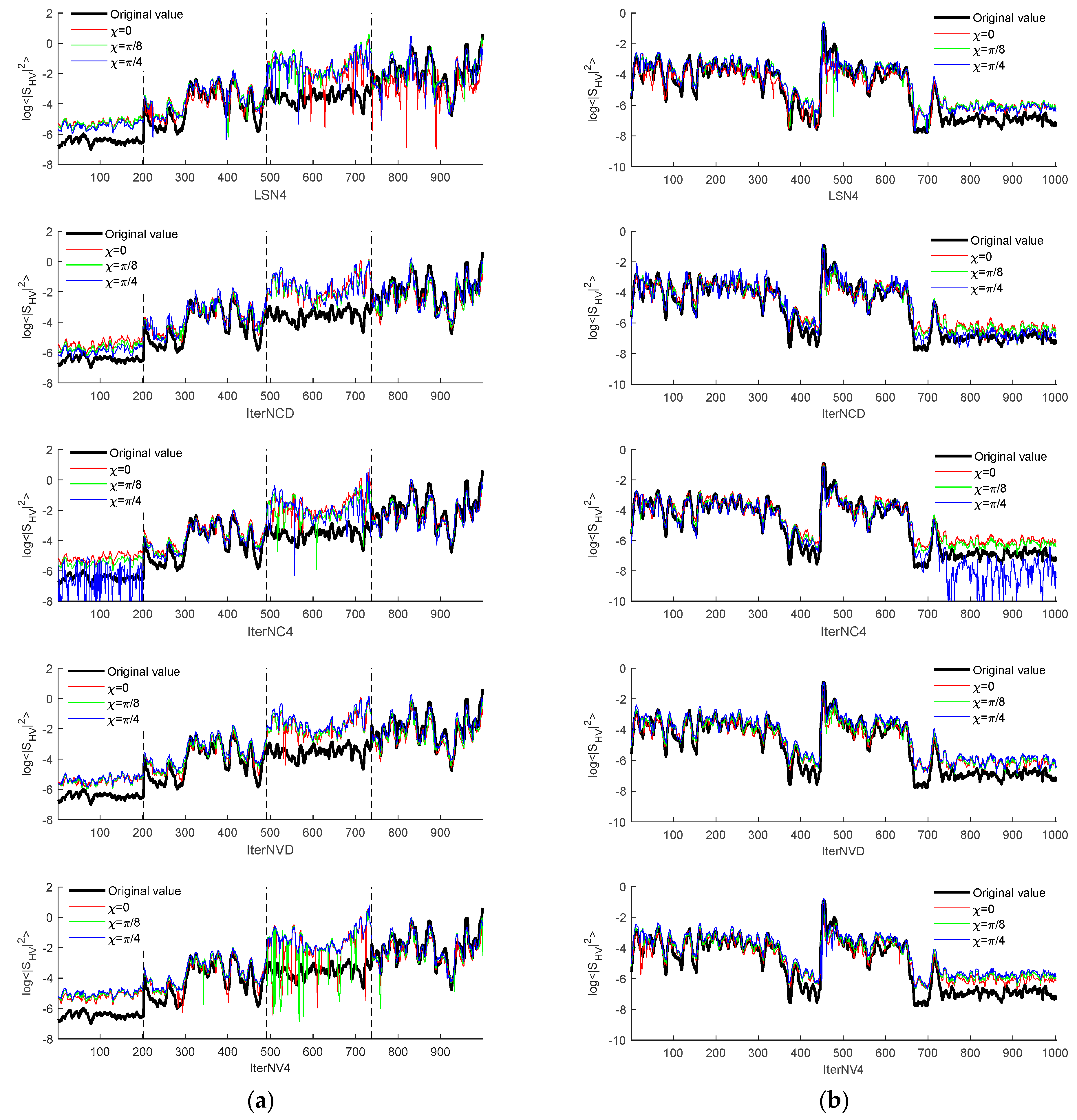
The pseudo quad-pol imagery reconstruction can be implemented via the combination of the reconstruction models and the LS-based or the iteration-based solving approach. The reconstruction model can be with either constant $N$, which is a pre-defined parameter, or variable $N$, which is updated during the iteration procedure. In Section 4.1, we formulated the reconstruction model and presented both the empirical and theoretical model parameters in Table 1. The empirical model is closely related to the observation scenarios and can only be applied to areas with a single terrain type, so we do not include the empirical model in the experiments. The Nord et al. variable $N$ model needs initial values for the iterative approach and is sensitive to the initialization [9], which cannot be embedded in the LS estimator. Thus, we only consider two reconstruction models, i.e., the $N=4$ model [7] and the decomposition-based model [12]. These two models can be combined with both the LS estimator and the iterative approach. For the iterative approach, different updating strategies can be applied to the model parameter $N$, either constant or variable with different initial values. Hence, from the explanation above, we consider 6 reconstruction algorithms, that is, the LS estimators with Souyris’s and Yin’ model parameters, the iterative approaches with constant Souyris’s and Yin’ model parameters, and the iterative approaches with Yin’s model in which $N$ is variable and initialized with $N=4$ as well as initialized by the CP ${\alpha }_s$- based decomposition method. The above algorithms are denoted in turn as LSN4, LSND, IterNC4, IterNCD, IterNV4, and IterNVD, respectively.

Experiments are conducted on the following aspects: (1) performances of the iterative and LS-based methods, (2) reconstruction accuracies of the reconstruction models, (3) reconstruction accuracies under different CP modes, and (4) comparison of the performances of CP data, pseudo quad-pol data, and FP data for multi-temporal agriculture field classification. Three CP modes, i.e., the linear π/4 mode ($\theta =\mathsf{\pi }/4,\chi =0$), an elliptical mode ($\theta =\mathsf{\pi }/4,\chi =\mathsf{\pi }/8$), and the left circular mode ($\theta =\mathsf{\pi }/4,\chi =\mathsf{\pi }/4$), are used for demonstration. For these CP modes, the transmit waves are balanced in amplitude, i.e., $\left|x\right|=\left|y\right|$, so the variable-N algorithm is applicable. The linear π/4 and circular modes are commonly considered imaging configurations. They are included so as to get comparable results with those found in the open literature.

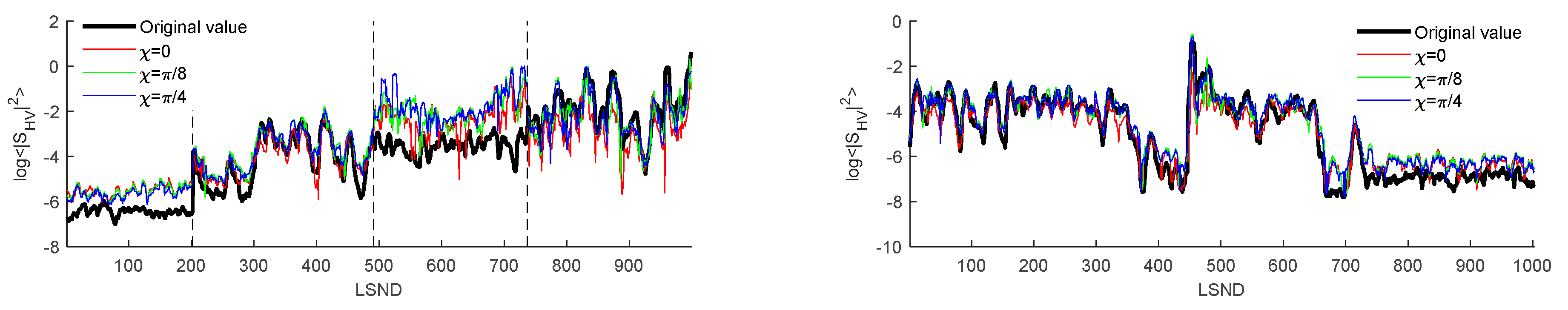
Reconstructed results for the line segments in Figure 2 are given in Figure 5. It shows that in general the results from the decomposition-based model is better than those from the $N=4$ model, no matter which solving approaches is used. For the variable $N$ methods, we again verify that the initialization affects the reconstructed results, especially for the circular CP mode, as can be observed from the last two rows in Figure 5. Initial values given by the ${\alpha }_s$-based decomposition generates better results than the initial guess with $N=4$. For the iterative methods with constant $N$, it shows that the $N=4$ model under the circular mode does not performs well for the ocean surface, as can be observed in the IterNC4 plots that the blue profiles for the ocean surface has larger variations. Results show that the iterative method with constant-$N$ estimated by the ${\alpha }_s$-based decomposition outperforms the other methods under the circular mode for the ocean surface. Compared to the iterative methods, the LS estimator is superior for reconstruction of the urban area data when combined with the decomposition-based model. In the LS-based method, the linear CP mode gives lower estimates for the cross-pol term as compared with the elliptical and circular CP modes for land areas. From Figure 5, it shows that the constant $N=4$ iterative method is not suitable for ocean surface reconstruction, especially in the circularly polarized mode. Comparatively, the constant-N method with N estimated from the ${\alpha }_s$-based decomposition (IterNCD) has the best reconstruction accuracy for ocean surface under the circular mode. While for land areas, the LS-based method LSND has the best result. However, for the urban area without obvious rotation, all methods tend to overestimate the cross-pol term. Further, results in Figure 5 also show that the decomposition-based model fit the urban areas better in both iterative and LS-based solving approaches, which is because the typical reflection asymmetry model, i.e., the helix scattering models, also satisfies the decomposition-based reconstruction model. However, the reflection asymmetric models do not agree with the N = 4 model.

Evaluation in terms of root mean square errors (RMSE) and percentages of the pixels that deviate from the real values by 5% of the total range are given in

Table 2. Quantitative evaluation for $\log \langle {\left|S_{\mathrm{HV}}\right|}^2\rangle$ and CPD by using the root mean square error (RMSE) and the percentage of pixels deviating from the real values by 5% of the total range. Three CP modes illustrated are $\left(\theta =\mathsf{\pi }/4,\chi =0\right)$, $\left(\theta =\mathsf{\pi }/4,\chi =\mathsf{\pi }/8\right)$, and $\left(\theta =\mathsf{\pi }/4,\chi =\mathsf{\pi }/4\right)$.

Data Sets	CP Modes	Rec. Errors	LSND	LSN4	IterNCD	IterNC4	IterNVD	IterNV4
ALOS-2 SF data	$\chi =0$	RMSE of $\log \langle {\left|S_{\mathrm{HV}}\right|}^2\rangle$	1.161	1.528	1.361	1.403	1.289	1.434
		RMSE of CPD	1.211	1.290	1.229	1.330	1.192	1.235
		|CPDc-CPD|>π/10	28.9%	36.7%	32.8%	39.8%	31.1%	34.4%
	$\chi =\mathsf{\pi }/8$	RMSE of $\log \langle {\left|S_{\mathrm{HV}}\right|}^2\rangle$	1.247	1.559	1.323	1.300	1.358	1.599
		RMSE of CPD	1.484	1.592	1.511	1.649	1.531	1.567
		|CPDc-CPD|>π/10	37.8%	46.3%	39.5%	41.3%	40.3%	42.3%
	$\chi =\mathsf{\pi }/4$	RMSE of $\log \langle {\left|S_{\mathrm{HV}}\right|}^2\rangle$	1.297	1.467	1.360	1.338	1.501	1.574
		RMSE of CPD	1.106	1.244	1.159	1.121	1.140	1.141
		|CPDc-CPD|>π/10	41.9%	41.4%	43.3%	43.1%	44.1%	42.4%
RS-2 Fuzhou data	$\chi =0$	RMSE of $\log \langle {\left|S_{\mathrm{HV}}\right|}^2\rangle$	0.637	0.781	0.658	0.762	0.658	0.805
		RMSE of CPD	0.639	0.698	0.662	0.733	0.635	0.662
		|CPDc-CPD|>π/10	13.9%	16.0%	16.3%	19.3%	15.7%	16.8%
	$\chi =\mathsf{\pi }/8$	RMSE of $\log \langle {\left|S_{\mathrm{HV}}\right|}^2\rangle$	0.608	0.788	0.571	0.638	0.680	0.902
		RMSE of CPD	0.726	0.756	0.715	0.765	0.729	0.755
		|CPDc-CPD|>π/10	22.9%	25.1%	20.2%	21.1%	21.9%	23.6%
	$\chi =\mathsf{\pi }/4$	RMSE of $\log \langle {\left|S_{\mathrm{HV}}\right|}^2\rangle$	0.534	0.711	0.535	0.827	0.783	0.941
		RMSE of CPD	0.578	0.630	0.591	0.583	0.576	0.588
		|CPDc-CPD|>π/10	20.2%	20.3%	21.6%	21.8%	20.4%	19.7%
RS-2 WF data	$\chi =0$	RMSE of $\log \langle {\left|S_{\mathrm{HV}}\right|}^2\rangle$	0.435	0.485	0.461	0.502	0.439	0.469
		RMSE of CPD	0.737	0.825	0.760	0.857	0.718	0.753
		|CPDc-CPD|>π/10	20.9%	24.1%	24.6%	28.9%	23.6%	25.2%
	$\chi =\mathsf{\pi }/8$	RMSE of $\log \langle {\left|S_{\mathrm{HV}}\right|}^2\rangle$	0.467	0.527	0.421	0.428	0.454	0.543
		RMSE of CPD	0.791	0.783	0.746	0.774	0.772	0.782
		|CPDc-CPD|>π/10	34.0%	36.3%	29.4%	30.8%	31.9%	34.1%
	$\chi =\mathsf{\pi }/4$	RMSE of $\log \langle {\left|S_{\mathrm{HV}}\right|}^2\rangle$	0.390	0.493	0.488	0.427	0.580	0.606
		RMSE of CPD	0.571	0.597	0.574	0.560	0.551	0.575
		|CPDc-CPD|>π/10	29.2%	27.7%	30.0%	29.6%	27.6%	26.6%

Rec. Errors = Reconstruction errors; CPDc = the reconstructed CPD; SF = San Francisco; RS = RADARSAT; WF = Wallerfing.

. $\langle {\left|S_{\mathrm{HV}}\right|}^2\rangle$ directly affects the reconstruction performances and CPD is associated with the identification of scattering mechanisms. RMSE is calculated for both $\langle {\left|S_{\mathrm{HV}}\right|}^2\rangle$ and CPD, and the pixel percentage of deviation is calculated for CPD. In Table 2, for each assessment index, the first two methods that are with best estimation results are highlighted. Reconstruction are performed under the aforementioned 3 CP modes for the test data sets. In total, each method is quantified 27 times. Results show that for the LSND, LSN4, IterNCD, IterNC4, IterNVD, and IterNV4 methods, the frequencies that those methods perform best are 21/27, 1/27, 10/27, 8/27, 13/27, and 2/27, respectively. The LS estimator with the decomposition-based model can provide the best overall results, and the variable-$N$ method initialized by parameters from the ${\alpha }_s$-based decomposition is in the second position.

In the LSND method, for the linear π/4 mode, the elliptical model with $\left(\theta ,\chi \right)=\left(\mathsf{\pi }/4,\mathsf{\pi }/8\right)$, and the circular mode, on average 0.98%, 0.6% and 0% pixels, respectively, cannot find minimums in the solution constraint. With the LSN4 method, for the 3 CP modes, 1.17%, 1.14%, and 1.83% pixels cannot find minimums within the constraint. This indicates that the decomposition-based model is more accurate to fit the CP data under different modes.

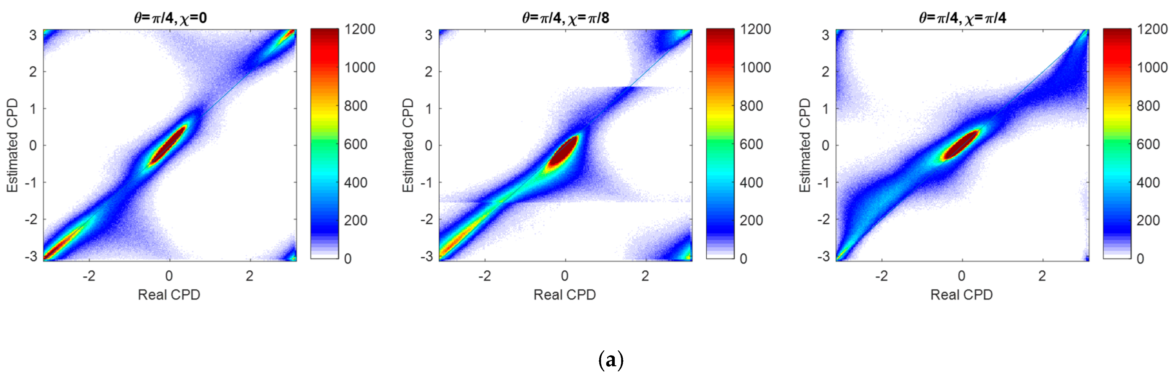
The reconstructed accuracy of CPD is another important factor to evaluate the reconstruction performance. On average, the LSND method performs best in phase reconstruction. By using the L-band ALOS-2/PALSAR data for illustration, CPDs estimated by LSND for the three CP modes are shown in Figure 6a. It shows that under the linear π/4 mode, most pixels distribute along the diagonal line, indicating a superior reconstruction result. The reconstructed $\langle {\left|S_{\mathrm{HV}}\right|}^2\rangle$ is evaluated in Figure 6b in terms of the relative error. Similar analysis results can be found in [14] (see Figure 5 and Figure 6) for the C-band RADARSAT-2 data over the same test site for the Linear CP mode. Figure 6b shows that for the urban area without obvious rotation, the linear π/4 mode has smaller relative errors compared to the other two modes, but still the relative error of city areas is larger than those of ocean surface and forested areas. For the rotated urban area, the linear π/4 mode has the larger relative errors and in contrast the circular mode performs best. Since for this test set, the rotated urban area and the forested areas are characterized by a similar cross-pol and co-pol ratio, i.e., ratio between the cross-pol intensity and the sum of co-pol intensities, it is expected that the circular mode would also perform better for the forested areas. Relative errors of the reconstructed $\log \langle {\left|S_{\mathrm{HV}}\right|}^2\rangle$ for the areas outlined in Figure 2c are listed in

Table 3. Relative errors of the reconstructed $\log \langle {\left|S_{\mathrm{HV}}\right|}^2\rangle$ for the outlined areas in Figure 2c by using the LSND method. The CP modes are with $\theta =\mathsf{\pi }/4$.

	Areas	Ocean	Forest	Urban Area 1	Urban Area 2	Tilted Urban Area
CP Mode
$\chi =0$		0.1607	0.1470	0.2548	0.5542	3.7927
$\chi =\mathsf{\pi }/8$		0.1602	0.1305	0.2965	0.6452	1.9128
$\chi =\mathsf{\pi }/4$		0.1410	0.1198	0.3746	0.7713	1.4856

. The quantitative result is consistent with the explanation for the results shown in Figure 6b.

Results in Figure 5 and Figure 6b, and Table 3 show that a same method performs differently for different terrain types when the CP mode varies. Since from Table 2, it is shown that apart from the LSND method, the IterNCD and IterNVD methods have relatively better overall reconstruction accuracies, in

Table 4. Relative errors of the reconstructed $\log \langle {\left|S_{\mathrm{HV}}\right|}^2\rangle$ for the outlined areas in Figure 2c by using (a) the IterNCD method, and (b) the IterNVD method. The CP modes are with $\theta =\mathsf{\pi }/4$.

	Areas	Ocean	Forest	Urban Area 1	Urban Area 2	Tilted Urban Area
CP Mode
(a)
$\chi =0$		0.1761	0.1310	0.3414	0.7410	3.4842
$\chi =\mathsf{\pi }/8$		0.1390	0.1197	0.3658	0.7551	2.5697
$\chi =\mathsf{\pi }/4$		0.1019	0.1541	0.4251	0.7931	1.6888
(b)
$\chi =0$		0.1708	0.1227	0.3065	0.7002	3.0527
$\chi =\mathsf{\pi }/8$		0.1759	0.1203	0.3549	0.7471	2.3744
$\chi =\mathsf{\pi }/4$		0.1886	0.1556	0.4343	0.8200	1.4945

we further show the relative errors of $\langle {\left|S_{\mathrm{HV}}\right|}^2\rangle$ for those methods. In combination with the profiles in Figure 5, it confirms that the IterNCD method is favorable for the circular mode to reconstruct the scattering coefficient of ocean surface. The combination use of the linear CP mode and the LSND method is better than any other combinations of the CP modes and the reconstruction algorithms for the urban areas which do not possess obvious rotation angles. For the forested and tilted urban areas, reconstruction results obtained from the circular mode are better, especially when LSND is used.

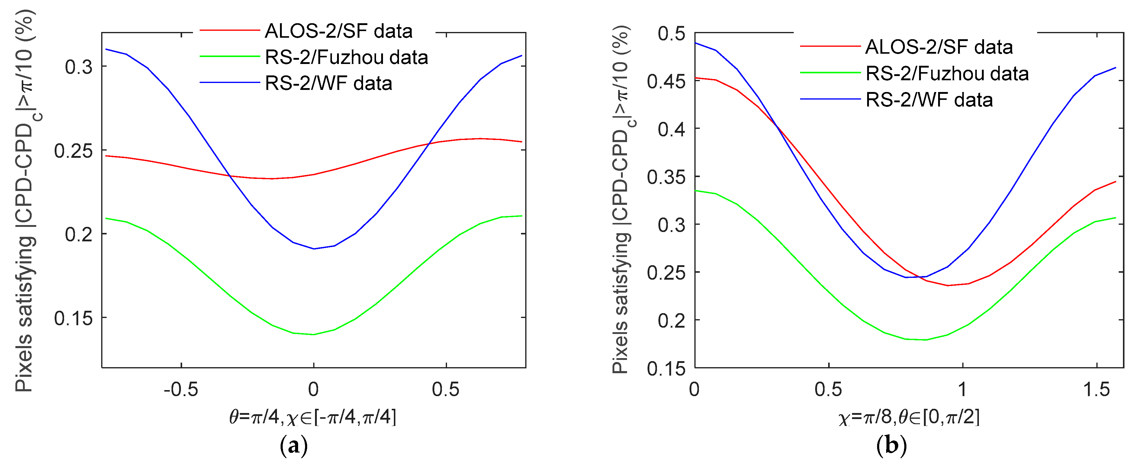
Table 2 shows that for all methods, the deviation percentage which evaluates the agreement of reconstructed and real CPDs is smallest in the linear π/4 mode. In combination with the scatter plots in Figure 6a, we found that the π/4 mode outperforms the other two CP modes in the reconstruction of the phase term. RMSE of CPD is larger for the π/4 mode is due to the period of 2π radians phase. When the real CPD is close to ±π, a small perturbation on the estimated $\langle {\left|S_{\mathrm{HV}}\right|}^2\rangle$ will lead to dramatic changes of ±2π in the estimated CPD (e.g., from −π to π or from π to −π), as can be observed in Figure 6a that in the π/4 mode a certain amount of pixels lies in the corners of (−π, π) and (π, −π). This results in larger RMSEs. For the other two test sets in Figure 2, distributions of the CPD estimated by LSND under the 3 CP modes are quite similar to those in Figure 6a. The omitted terms in (5) by assuming reflection symmetry has different impacts on CPD when the CP mode varies. In Figure 7, assuming that $\langle {\left|S_{\mathrm{HV}}\right|}^2\rangle$ is perfectly reconstructed, we show variation of the deviation percentages of the reconstructed CPD with the varying CP modes. It shows that for all test data sets, when the transmit wave channel amplitude is balanced, the estimated CPD is least affected by the assumption of reflection symmetry in the linear mode. The case that the channel amplitudes of the transmit wave are imbalanced is also tested. We found that the more the CP mode is linearly polarized, the closer the reconstructed CPD is to the real value. This implies that if applications are based on the pseudo quad-pol images and the algorithms applied subsequently are CPD-based, results obtained from the linear π/4 mode may be expected to be closer to that of the FP mode. For example, if CPD is used to discriminate surface and double-bounce scattering such as in the application of Freeman-Durden’s decomposition, the overall agreements in |CPD|>π/2 between the FP data (ALOS-2/PALSAR SF data) and the pseudo-FP data reconstructed by LSND are 88.75% and 84.72%, respectively, for the linear π/4 and circular modes, and by IterNVD the agreements are 89.35% and 81.34%, respectively.

Another application is carried out for example, which is the crop type classification by using the RS-2 Wallerfing data. The iterative Wishart classifier [23] is used to perform the classification, with 5% pixels randomly selected as the training samples based on ground data. For each data set, same training samples are used for all the subsequent experimental implementation. Although several studies [3,4,24] have been conducted on the comparison of the performances of CP, pseudo quad-pol, and FP data for terrain type classification, there is rare study giving a clear illustration on the variation of the overall classification accuracies under different circumstances. In Figure 8, by using the Wallerfing data acquired by RADARSAT-2 on May 28, 2014, we tested the classification performances of the reconstructed data, the original 2 × 2 CP covariance matrix data, and the original 3 × 3 FP covariance matrix data. The reconstructed $\langle {\left|S_{\mathrm{HV}}\right|}^2\rangle$ is assumed to be $r{\mathrm{X}}_{\min }$ with $r\in \left[\begin{array}{cc}0.1& 1\end{array}\right]$, where ${\mathrm{X}}_{\min }$ is the upper bound for the cross-pol term in estimation. By this means, the pseudo FP data is accordingly reconstructed. It shows that compared to the original CP data, the reconstructed data with the accurately estimated $\langle {\left|S_{\mathrm{HV}}\right|}^2\rangle$ greatly improve the classification accuracy, especially for the linear CP mode, in which case the classification accuracy is improved by 5.3%. For the circular mode, when the estimated $\langle {\left|S_{\mathrm{HV}}\right|}^2\rangle$ is too large, the classification accuracy will deteriorate dramatically. In Figure 8, we did not give the classification rates in the cases of $\langle {\left|S_{\mathrm{HV}}\right|}^2\rangle {}_c=0.9{\mathrm{X}}_{\min }$ and $\langle {\left|S_{\mathrm{HV}}\right|}^2\rangle {}_c={\mathrm{X}}_{\min }$ for the circular mode, because in both cases the term $\langle {\left|S_{\mathrm{HH}}-S_{\mathrm{VV}}\right|}^2\rangle /2$ of the reconstructed coherency matrix is close to 0 or even negative for a certain amount of pixels, for instance, 15% pixels in the $r=0.9$ case and 23% in the $r=1$ case. However, if the estimation is accurate, Figure 8 shows that in general the circular mode is better for agriculture field classification.

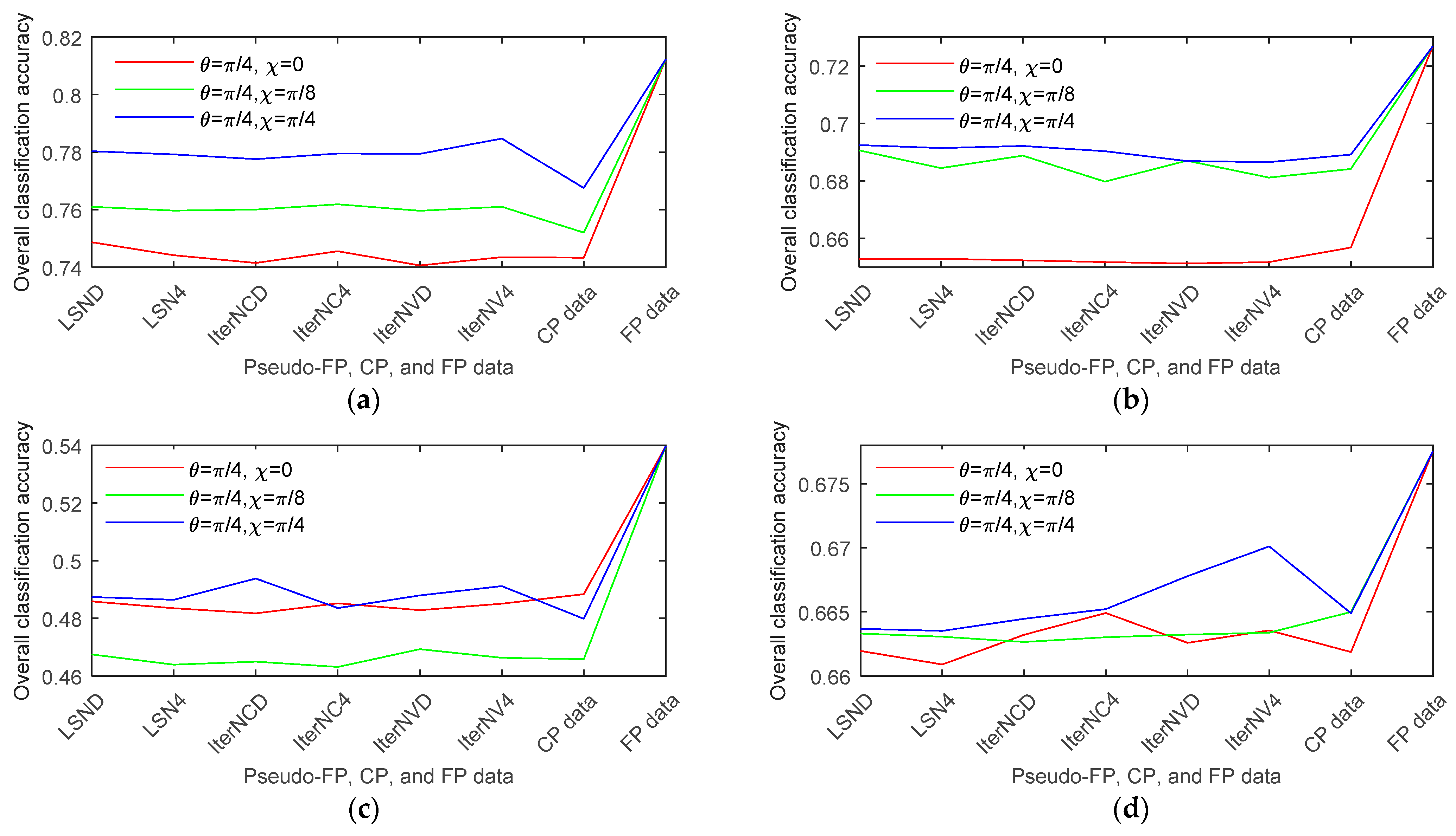
Next we consider the performances of the pseudo quad-pol data sets reconstructed via the test methods for multi-phase crop classification. The overall classification accuracies of the 6 methods, and those of the original CP as well as the FP data are shown in Figure 9. We observe that the circular mode performs best, which is in accordance with the analysis in Figure 8. However, for the multi-phase data sets, due to different phenology periods and disturbance of environmental changes, the best method evaluated in terms of overall classification accuracy varies. However, in general, data reconstructed by the iterative approach with the decomposition-based model provides comparatively better and stable classification accuracies if the Wishart classifier is applied. It also shows that classification carried out on the reconstructed data is better than that on the original CP data.

7. Summary and Discussion

In this study, based on the formalized CP descriptors which was one of the recent developed works, we unified the current pseudo quad-pol imagery reconstruction models into two frameworks, which are the LS error model and the iterative approach, to estimate the FP scattering coefficients. By inducing this formalism, the system of nonlinear equations is parameterized by the transmit wave coefficients, and the most important is the co-polarized coherence has a unified form for the general CP mode. By this means, the two unknown solving approaches can be combined with any reconstruction models (either empirical or theoretical $N$ models) for an arbitrary CP mode. The decomposition-based variable $N$ method is also extended for the CP mode which is with balanced transmitted wave channel amplitudes.

Experiments were carried out on 6 data sets to demonstrate the performances of reconstruction models and solving approaches. On average, the decomposition-based model is more adaptive and provides better results than the $N=4$ model. Results showed that by using a same reconstruction method the linear mode has better reconstruction accuracy in the cross-pol term than the circular mode for urban areas. While the circular mode always performs better for areas not dominated by double-bounce scattering, especially for ocean surface. If evaluated in terms of CPD, the linear π/4 mode always outperforms the circular mode. We also carried out same experiments on several other data sets in addition to the data sets presented in this paper, and similar conclusions were obtained.

Most reconstruction algorithms, including the methods summarized and extended in this study, were proposed based on reflection symmetry. If backscatter of scatterers does not follow the reflection symmetric assumption, then the reconstructed results will have a larger estimation error. This is caused by the omitted terms, which are assumed to be 0 by reflection symmetry but actually are comparable to the cross-pol term, thus leading to larger relative errors. The reconstruction model parameter$N$ is the key factor for good reconstruction. If N is accurate, both the LS-based and the constant-N iterative methods can achieve a perfect reconstruction. At this point the variable-N method is no longer preferable. However, except the empirical N, there are only 2 theoretical methods that can give a prior estimation for N, i.e., the N = 4 and the N from the ${\alpha }_s$-based decomposition. The N = 4 model applies well for areas dominated by volume scattering, but this application situation is very restricted. $N$estimated from the ${\alpha }_s$-based decomposition is more adaptive to the observation scenarios. However, since the CP mode only measures partial information of the backscattering space, the difference of the decomposed powers from CP and FP data is inevitable. Improvement on the accuracy of $N$ still needs further studies, e.g., by developing semi-empirical models.

References

- Lee, J.S.; Pottier, E. Polarimetric Radar Imaging from Basics to Applications; CRC Press: Boca Raton, FL, USA, 2009; Chapters 2–3; pp. 31–98. [Google Scholar]
- Raney, R. Hybrid-polarity SAR architecture. IEEE Trans. Geosci. Remote Sens. 2007, 45, 3397–3405. [Google Scholar] [CrossRef] [Green Version]
- Charbonneau, F.J.; Brisco, B.; Raney, R.K.; McNairn, H.; Liu, C.; Vachon, P.W.; Shang, J.; DeAbreu, R.; Champagne, C.; Merzouki, A.; et al. Compact polarimetry overview and applications assessment. Can. J. Remote Sens. 2010, 36, S298–S315. [Google Scholar] [CrossRef]
- Ohki, M.; Shimada, M. Large-area land use and land cover classification with quad, compact, and dual polarization SAR data by PALSAR-2. IEEE Trans. Geosci. Remote Sens. 2018, 56, 5550–5557. [Google Scholar] [CrossRef]
- Shirvany, R.; Chabert, M.; Tourneret, J.-Y. Ship and oil-spill detection using the degree of polarization in linear and hybrid/compact dual-pol SAR. IEEE J. Sel. Top. Appl. Earth Obs. Remote Sens. 2012, 5, 885–892. [Google Scholar] [CrossRef] [Green Version]
- Yin, J.; Yang, J.; Zhou, Z.-S.; Song, J. The extended Bragg scattering model-based method for ship and oil-spill observation using compact polarimetric SAR. IEEE J. Sel. Top. Appl. Earth Obs. Remote Sens. 2015, 8, 3760–3772. [Google Scholar] [CrossRef]
- Souyris, J.; Imbo, P.; Fjørtoft, R.; Mingot, S.; Lee, J.-S. Compact polarimetry based on symmetry properties of geophysical media: The π/4 mode. IEEE Trans. Geosci. Remote Sens. 2005, 43, 634–646. [Google Scholar] [CrossRef]
- Nord, M.; Ainsworth, T.; Lee, J.-S.; Stacy, N. Comparison of compact polarimetric synthetic aperture radar modes. IEEE Trans. Geosci. Remote Sens. 2009, 47, 174–188. [Google Scholar] [CrossRef]
- Collins, M.; Denbina, M.; Atteia, G. On the reconstruction of quad-pol SAR data from compact polarimetry data for ocean target detection. IEEE Trans. Geosci. Remote Sens. 2013, 51, 591–600. [Google Scholar] [CrossRef]
- Collins, M.; Denbina, M.; Minchew, B.; Jones, C.; Holt, B. On the use of simulated airborne compact polarimetric SAR for characterinzing oil-water mixing of the Deepwater Horizon oil spill. IEEE J. Sel. Top. Appl. Earth Obs. Remote Sens. 2015, 8, 1062–1077. [Google Scholar] [CrossRef]
- Li, Y.; Zhang, Y.; Chen, J.; Zhang, H. Improved compact polarimetric SAR quad-pol reconstruction algorithm for oil spill detection. IEEE Geosci. Remote Sens. Lett. 2014, 11, 1139–1142. [Google Scholar] [CrossRef]
- Yin, J.; Moon, W.M.; Yang, J. Model-based pseudo quad-pol reconstruction from compact polarimetry and its application to oil-spill observation. J. Sens. 2015, 2015, 1–8. [Google Scholar] [CrossRef]
- Yin, J.; Yang, J. Multi-polarization reconstruction from compact polarimetry based on modified four-component scattering decomposition. J. Syst. Eng. Electron. 2014, 25, 399–410. [Google Scholar] [CrossRef]
- Yin, J.; Papathanassiou, K.; Yang, J.; Chen, P. Least-squares estimation for pseudo Quad-Pol image reconstruction from linear compact polarimetric SAR. IEEE J. Sel. Top. Appl. Earth Obs. Remote Sens. 2019, 12, 3746–3758. [Google Scholar] [CrossRef]
- Van Zyl, J.; Kim, Y. Synthetic aperture radar polarimetry. In JPL Space Science and Technology Series; John Wiley and Sons: Hoboken, NJ, USA, 2012; Chapter 2; pp. 27–83. [Google Scholar]
- Freeman, A.; Durden, S.L. A three-component scattering model for polarimetric SAR data. IEEE Trans. Geosci. Remote Sens. 1998, 36, 963–973. [Google Scholar] [CrossRef] [Green Version]
- Freeman, A. Fitting a two-component scattering model to polarimetric SAR data from forests. IEEE Trans. Geosci. Remote Sens. 2007, 45, 2583–2592. [Google Scholar] [CrossRef]
- Yin, J.; Papathanassiou, K.; Yang, J. Formalism of compact polarimetric descriptors and extension of the ∆αB/αB method for general compact-pol SAR. IEEE Trans. Geosci. Remote Sen. 2019, 57, 10322–10335. [Google Scholar] [CrossRef]
- Yin, J.; Yang, J. Target decomposition based on symmetric scattering model for hybrid polarization SAR imagery. IEEE Geosci. Remote Sens. Lett. 2020, in press. [Google Scholar] [CrossRef]
- Cloude, S.; Goodenough, D.; Chen, H. Compact decomposition theory. IEEE Geosci. Remote Sens. Lett. 2012, 9, 28–32. [Google Scholar] [CrossRef]
- Sabry, R.; Vachon, P.W. A unified framework for general compact and quad polarimetric SAR data and imagery analysis. IEEE Trans. Geosci. Remote Sens. 2014, 52, 582–602. [Google Scholar] [CrossRef]
- Lee, J.-S. Refined filtering of image noise using local statistics. Comput. Vis. Graph. Image Process. 1981, 15, 380–389. [Google Scholar] [CrossRef]
- Lee, J.-S.; Grunes, M.R.; Ainsworth, T.L.; Du, L.-J.; Schuler, D.L.; Cloude, S.R. Unsupervised classification using polarimetric decomposition and the complex Wishart classifier. IEEE Trans. Geosci. Remote Sens. 1999, 37, 2249–2258. [Google Scholar]
- Lardeux, C.; Frison, P.-L.; Tison, C.; Souyris, J.-C.; Stoll, B.; Fruneau, B.; Rudant, J.-P. Classification of tropical vegetation using multifrequency partial SAR polarimetry. IEEE Geosci. Remote Sens. Lett. 2011, 8, 133–137. [Google Scholar] [CrossRef]
Figure 1.
Outline of the study.
Figure 2.
Pauli-basis images. (a) The Wallerfing data (28 May 2014), RADARSAT-2. (b) The crop type information of the Wallerfing area. (c) The San Francisco data, ALOS-2/PALSAR. Areas outlined by green, orange, and dark red are denoted as urban 1, urban 2, and tilted urban areas. (d) The Fuzhou data, RADARSAT-2.
Figure 3.
Variation of the overall agreement between and with the relative phase of the transmit wave . (a) Fuzhou data, RADARSAT-2, (b) San Francisco data, ALOS-2/PALSAR.
Figure 4.
Percentage of pixels (the Fuzhou data) that satisfy the bound constraint for two types of CP cases. (a) Transmit waves with balanced amplitudes, (b) transmit waves with imbalanced amplitudes.
Figure 5.
Estimate profiles for along the transect lines in Figure 2. (a) ALOS-2/PALSAR San Francisco data, where the four transect lines indicate data from ocean surface, forests, urban areas without obvious rotation, and tilted urban areas, respectively; (b) RADARSAT-2 Fuzhou data.
Figure 6.
(a) Scatter plots of the reconstructed CPD from the LSND method. (b) Relative errors of the reconstructed , defined by . ALOS-2/PALSAR San Francisco data.
Figure 7.
Variation of the percentage of pixels that deviate from the perfect reconstruction by 5% with the varying CP modes. (a) The CP mode with . (b) The CP mode with .
Figure 8.
Variation of the overall classification accuracies with different polarimetric data sets, including pseudo-FP data with different reconstruction accuracies, where the estimated is designed to be varying between [0.1Xmin Xmin], the pseudo quad-pol data with perfectly estimated , the 2 × 2 CP covariance matrix data, and the 3 × 3 FP covariance matrix data (RS-2 WF data obtained on May 28, 2014). Xmin is the upper bound in the LS estimation for , where .
Figure 9.
Overall classification rates for the agriculture field by using the pseudo quad-pol data reconstructed by the LS-based and iterative methods, the original 2 × 2 CP covariance matrix data, and the FP data. Data acquired on (a) 20140528, (b) 20140621, (c) 20140715, and (d) 20140808.