Article

Modelling and Comparing Shading Effects of 3D Tree Structures with Virtual Leaves

by
Rafael Bohn Reckziegel
*,
Elena Larysch
,
Jonathan P. Sheppard
,
Hans-Peter Kahle
and
Christopher Morhart
Chair of Forest Growth and Dendroecology, University of Freiburg, Tennenbacher Str. 4, 79106 Freiburg, Germany
*
Author to whom correspondence should be addressed.
Submission received: 7 December 2020 / Revised: 24 January 2021 / Accepted: 28 January 2021 / Published: 2 February 2021

Abstract

:
Reduced solar radiation brought about by trees on agricultural land can both positively and negatively affect crop growth. For a better understanding of this issue, we aim for an improved simulation of the shade cast by trees in agroforestry systems and a precise estimation of insolation reduction. We present a leaf creation algorithm to generate realistic leaves to be placed upon quantitative structure models (QSMs) of real trees. Further, we couple it with an enhanced approach of a 3D model capable of quantifying shading effects of a tree, at a high temporal and spatial resolution. Hence, 3D data derived from wild cherry trees (Prunus avium L.) generated by terrestrial laser scanner technology formed a basis for the tree reconstruction, and served as leaf-off mode. Two leaf-on modes were simulated: realistic leaves, fed with leaf data from wild cherry trees; and ellipsoidal leaves, having ellipsoids as leaf-replacement. For comparison, we assessed the shading effects using hemispherical photography as an alternative method. Results showed that insolation reduction was higher using realistic leaves, and that the shaded area was greater in size than with the ellipsoidal leaves or leaf-off conditions. All shading effects were similarly distributed on the ground, with the exception of those derived through hemispherical photography, which were greater in size, but with less insolation reduction than realistic leaves. The main achievements of this study are: the enhancement of the leaf-on mode for QSMs with realistic leaves, the updates of the shadow model, and the comparison of shading effects. We provide evidence that the inclusion of realistic leaves with precise 3D data might be fundamental to accurately model the shading effects of trees.

Graphical Abstract

1. Introduction

Established plants act as physical ecosystem engineers that directly or indirectly control the availability of resources to other organisms [1], for example, trees casting shade over food crops. Although shade is frequently treated simply in its literal sense as low light conditions [2], in a more general and ecological sense, it involves a wider range of environmental factors (altered atmospheric and substrate conditions) with various effects on plants (e.g., biotic interactions). As plant growth is driven by these factors and effects, i.e., resources (light, water, and nutrients) and conditions (temperature and shading), aside from specific plant traits, a change in quantity or quality of any of these factors triggers a change in plant growth. Thus, increasing the knowledge on resources availability, control, and modulation effects of the tree component, such as with a precise assessment of distribution of incoming solar radiation around a tree canopy, can aid a better understanding of resource dynamics, crop performance, and organisms’ interrelations.
Ecological habitats and production systems can be described in terms of their structural components. Structural diversity is unarguably poor in monocropping agricultural systems. In any productive system, an increase in structural diversity generally correlates with an increase in the complexity of the interdependencies of the individual elements. The latter being especially the case in complex ecosystems such as forests, as well as in integrated land-management solutions such as agroforestry systems (AFS).
AFS are combinations of woody perennials (i.e., trees) growing deliberately together with agricultural crops on the same land unit, and result in a significant interaction of the many system components [3,4,5,6]. For such systems, increased knowledge regarding the efficiency of resource utilisation is of utmost necessity. Eichhorn et al. [7] consider light being the primary limiting factor for the successful establishment and growth of intercrops in AFS. As the share of incoming solar radiation available to the plants is largely dependent of the structures found in a given landscape, a detailed assessment of the tree architecture could help to investigate the influence of trees on the radiation regime and their subsequent interaction with crops. Since the supply of solar radiation energy is equally essential for the growth of trees and crops, estimations of its spatial and temporal variation in the AFS must be considered for an optimised management. On one hand, a significant reduction of light interception for the agricultural crops growing closely to trees can result in a drastic reduction of crop productivity [8], especially in case of light-demanding species; on the other hand, under high-radiation conditions, more shade tolerant crop species could benefit from shading [9]. Due to the high importance of “light”, we focus on the influence of scattered trees in the radiation regime, by modelling the tree shading effects, quantifying the size and magnitude of insolation reduction. In Table 1, valuable concepts, terminologies, and definitions are summarised.
The measurement of light has a long tradition and is of high interest in environmental physics as well as in plant ecology [11]. To date, several techniques have been used to assess the share of incoming solar radiation under plant canopies. For the direct measurement of the light conditions different types of pyranometers were applied, while for indirect measurements devices such as the LAI-2000 Plant Canopy Analyser can be used to gather information about the leaf area index (LAI) of trees and forests [12].
The use of hemispherical photography is probably one of the most widely used indirect methods for gaining information on light conditions within wooded landscapes utilising a fisheye lens for whole sky photographs, a technique proposed nearly 100 years ago [13]. Evans and Coombe [14] were some of the first researchers applying it to a forest stand for measuring the direct and indirect radiation. Several follow-up studies appeared during the last decades and its applicability within other fields has also been tested. Comparative studies between hemispherical photography and other light sensors have been conducted by, e.g., [15,16,17,18]. This fact together with the ease of handling, the low price and the advantage of capturing all hemispherical directions simultaneously, are the main reasons for the broad application of this method. Light transmission measurements have already been undertaken using hemispherical photography in AFS [19].
A more advanced, and arguably more precise approach is the modelling of the light or radiation regime around trees based on three-dimensional (3D) structures. Dupraz and Liagre [20] replaced the crown with an ellipsoid for modelling the light distribution in AFS. This approach was further refined by Talbot and Dupraz [21] including additional parameters such as a leaf clumping coefficient and the shading effect of stem and branches. Alternative 3D models have also been developed by other groups, but they are all constrained by the scarce richness of details on the assessment [22,23,24,25,26]. Schmidt et al. [26] used a block with dimensions of 30 × 30 m and height of 20 m as a replacement of a forest edge to simulate shading in the field-to-forest transition zones of agricultural fields and estimate crop yields. Though an effort to represent the shading of a cluster of trees, the approach is lacking details of actual tree structures.
During the last decade the use of terrestrial laser scanners (TLS) has opened up new possibilities for the 3D modelling of the shade cast by trees [27,28,29,30,31,32]. While the other abovementioned 3D models rely on simplified 3D structures, TLS is supplying users with realistic and detailed 3D data of trees. Likewise, TLS approaches are superior to several conventional canopy analyses with optical methods, since they enable detailed coverage of vegetation surface with properly designed multi-scan sampling [33].
On the modelling of shade cast by trees, a recurrent strategy has been scanning trees with a TLS during the vegetation period and processing voxel data with ray tracing algorithms. At the attempt to increase the accuracy of voxel-based models arose difficulties in handling occlusion within the 3D data, due to insufficient information of the inner crown structure and vegetation clumping [28,31]. On the use of the voxel-based approach, an auspicious technique was presented by van der Zande et al. [27], where leaf area density could be directly derived by transforming TLS data into small leaf-sized voxels.
An alternative for modelling the shade cast by trees is by scanning deciduous trees under leafless conditions (e.g., during winter dormancy), reconstructing tree architecture with cylinder-based algorithms and adding leaf substitutes in a computer environment. Such approaches allow for the simulation of the shading effect of trees in a leaf-on mode. This technique was chosen by Rosskopf et al. [32] using a tree-cylinder model created with the software “SimpleTree” [34,35] coupled with ellipsoids as replacement for leaves. Other models reconstructing tree architecture with cylinders as geometric primitives exist [36,37,38,39]. They are often named quantitative structure models (QSMs) and contain accurate topological, geometrical and volumetric tree properties. “TreeQSM” [37,40,41] has been a popular method for modelling tree structures. Meanwhile, algorithms to insert leaves or needles as virtual structures into QSMs (produced with TreeQSM), and according to an arbitrary distribution exist [42]. In addition, the use of QSMs could offer the option to include TLS information concerning tree growth [43,44,45] and integrate it within the modelling approach.
We present a leaf creation algorithm (LCA) aiming at an improved simulation of the shade cast by individual trees for the estimation of its shading effect within a defined time-period. In this study, to virtually create leaves, the LCA is fed with species-specific leaf parameters derived for wild cherry trees (Prunus avium L.) growing in an AFS within southern Germany. The novelty of this approach is to use QSMs augmented with realistic leaves to compute shadow projections. We apply the new LCA to six trees and use an enhanced 3D modelling approach (named “shadow model”) capable of quantifying tree shading effect at high temporal and spatial resolution. Additionally, we simulate the shading effects for other leaf modes and compare the results with those achieved with hemispherical photography, as an alternative approach.
Our hypothesis is that a more realistic leaf-on mode (created by applying the LCA) does affect the simulated insolation on the surroundings of single-trees. Furthermore, our method is expected to be more accurate than concurrent methods for estimating spatial and temporal distribution of the shade cast by trees, and the correspondent insolation on the ground. The future validation of our shadow model will require the conduction of field assessment and tuning of model parameters. We showcase tree shading effects and gained insights on the accuracy of our method. The evidence gathered in this paper can be strategically used for planning and designing integrated tree-crop agricultural systems, in any landscape where light distribution is of concern, and for future development of specific and/or generalist methods on this study field.

2. Materials and Methods

2.1. Site Description and Trees

We selected six wild cherry trees (Prunus avium L.) growing in AFS in the vicinity of Eichstetten (48°06′26.3″N 7°43′53.6″E, 193 m a.s.l.), in the Kaiserstuhl region of southwest Germany. The trees have deciduous character, are growing free of competition of other trees and are scattered in agricultural fields cultivated with different crops; it is likely that the individual trees have received various silvicultural treatments during their lifespan, thus altering the growth, development, and actual structure. At the time of measurements (April 2019), the trees had heights ranging between 6 and 9 m and diameters at breast height (DBH) of 18 to 27 cm. The slope of the terrain at the scanned tree locations on the tree locations was considered flat (0–2%).
Within the Kaiserstuhl region, average annual direct normal radiation is 4158 MJ m−2 (11.39 MJ m−2 day −1) and annual global horizontal irradiation is 4402 MJ m−2, or 12.06 MJ m−2 day−1 [46]. The local climate is temperate and mild with a mean annual air temperature of 11.2 °C and a mean annual precipitation sum of 710 mm ensuring suitable growing conditions for trees [47]. The local soils consisting of periglacial loess which show a high-water permeability and low water storage capacity. As a consequence, the upper soil layers can be dry in summers experiencing low precipitation.

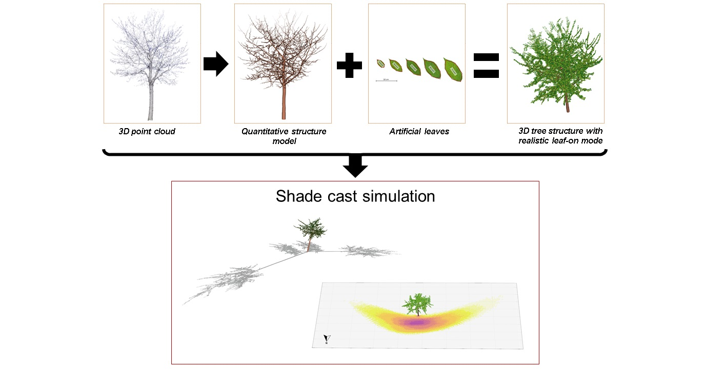
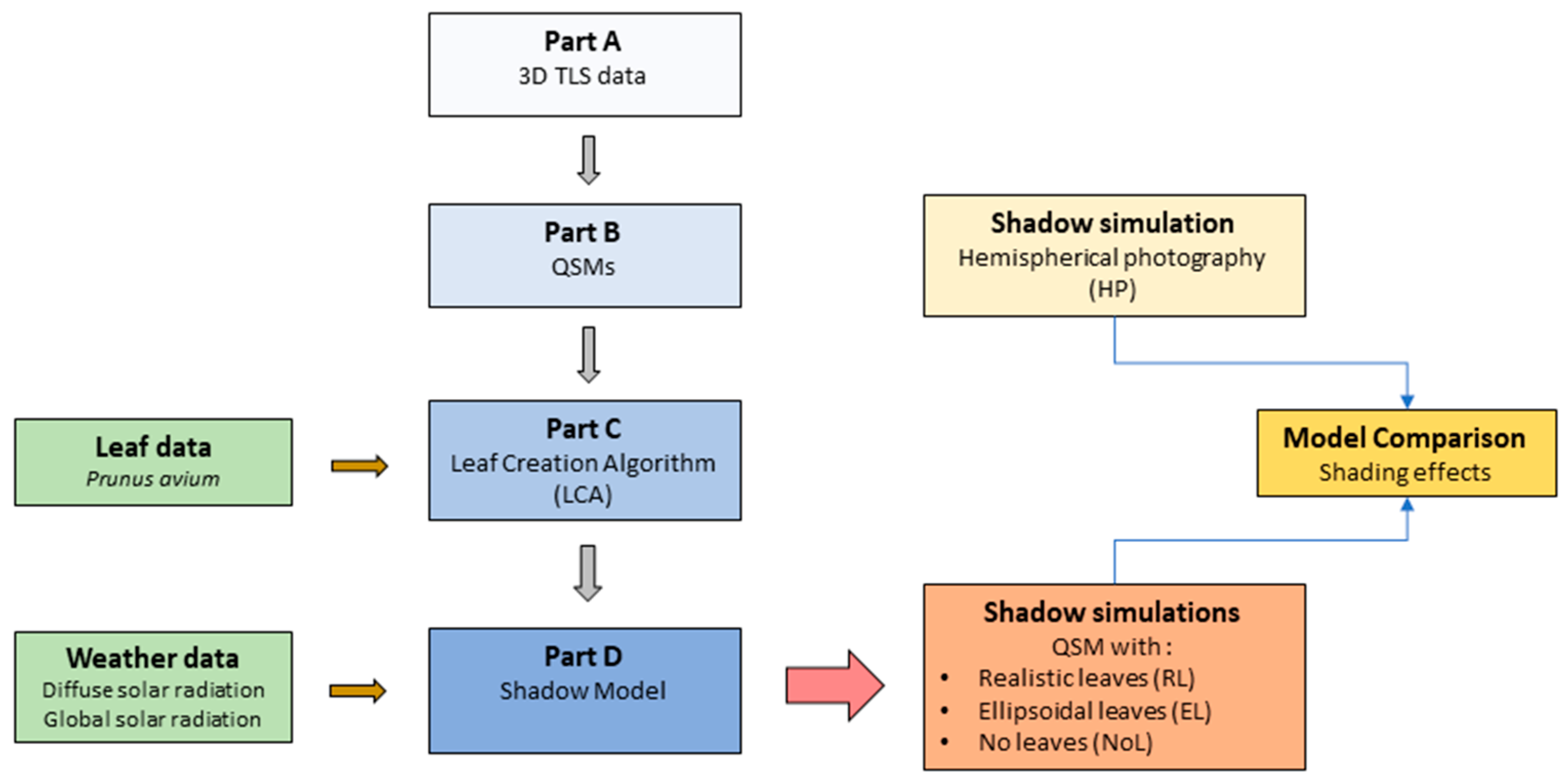
2.2. Overview of the Modelling Steps

The development of the shadow model can be divided in four parts (Parts A–D, see Figure 1):
  • Part A: Collection of 3D TLS data, processing and tree segmentation;
  • Part B: Creation of quantitative structure models (QSMs), representative of tree structures;
  • Part C: Introduction of the leaf creation algorithm (LCA) and its application;
  • Part D: Application of the shadow model using solar radiation data.
  • Part A: Collection of 3D TLS Data, Processing and Tree Segmentation
To update our shadow model, the six wild cherry trees were scanned with a TLS Faro Focus 3D S120 (FARO Technologies, Inc.; Lake Mary, FL, USA) in early spring (April 2019), under windless and leaf-off conditions, for a better visibility of the woody compartments of the trees [48]. The scanned tree surface is representative of the last growing season. We used a multiple scan approach with four scan positions around each tree, 90° degrees apart (azimuth angle) and at a distance of 10 m from the base of the tree. TLS device sampling parameters were set to ¼ for “resolution” and 4x for “quality”. A minimum of five reflective targets were set out around each tree to merge the multiple scans. The scans were registered using the software Faro Scene 6.2.4.30 (FARO Technologies, Inc.; Lake Mary, FL, USA) with a reported mean point error below 4 mm. Duplicated points were eliminated with a “low” search radius. In the following step, tree point clouds were manually extracted; this step was straightforward as trees had no direct neighbours or hindering obstacles. Lastly, we filtered the point clouds to remove noise points and outliers in CloudCompare v2.10.2 [49].
  • Part B: Creation of Quantitative Structure Models (QSMs)
The processed and filtered single-tree point clouds served as basis for reconstructing the architecture of trees using the MATLAB implementation of TreeQSM version 2.3 [37]. In the 3D reconstruction of QSMs, trees are modelled as a hierarchical collection of cylinders (e.g., geometric primitives) fitted to local details of the single-tree point cloud.
To optimise QSMs, we tested 32 combinations of key model input parameters (among them, cover patch diameter d, and relative cylinder length lcyl) and produced 15 models for each possible combination of inputs to select the best model, define the optimised parameters, and to assess the robustness of the reconstruction method and uncertainty of results [41,50]. The mean point-cylinder-model-distance was used as suitable metric for the optimisation [51]. All QSMs were reconstructed with the same optimised input parameters: in the first cover set d was 15 cm; for the second cover, the minimum and maximum d were 1 cm and 5 cm, respectively; lcyl was 3.5. The uncertainty of QSM-parameters stayed below 10% (CV; coefficient of variation) for each of the six trees. The regular, cylindrical-like, stem base of the trees did not require additional triangulation.
The QSM-derived tree parameters for the scanned trees are presented in Table 2. Trees were similar in terms of DBH and height, while total tree and branch volume, cylinder and branch counts, revealed the more complex structures hold by trees Pa_2, Pa_4 and Pa_5. We identified Pa_6 as the least elaborate tree structure. In addition, the count of branches and accumulated branch length are important as realistic leaves are placed along the branch-cylinders by the LCA (details in Section 2.2 Part C).
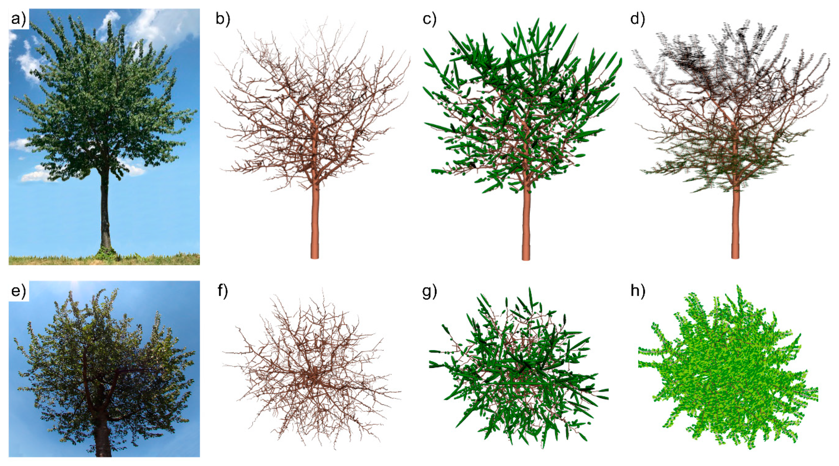
The QSMs play a central role in our shadow model, as they provide the basic topological structure to which virtually created leaves are attached. The processing steps are illustrated in Figure 2: a photograph of one wild cherry tree (Figure 2a); the QSM of that tree (Figure 2b); the modelled leaf-on mode with ellipsoidal leaf-replacements (Figure 2c); the new leaf-on mode using realistic leaves (Figure 2d); photograph of the crown for the four models as a worm’s eye view (Figure 2e); bird’s eye views of the QSM, QSM with ellipsoidal leaf-replacement and with realistic leaves, respectively (Figure 2f–h). The full description of the new leaf-on mode and the details of the enhanced shadow algorithm are presented in Section 2.2 Part C and Part D, respectively; the use of these 3D structures for simulating the shading effects is described in Section 2.3. A video-visualisation of the 3D structure of tree Pa_5, the QSM and leaf modes is found in Supplementary File S1.
  • Part C: Leaf Measurements and Leaf Creation Algorithm (LCA)
In July 2018, leaves were collected from felled wild cherry trees for generating data to serve as basis for the virtual creation of leaves on overlaying the QSMs in a computer environment. The realistic leaves were an attempt to represent carefully the leaf topology of wild cherry trees, and were used as the RL leaf-on mode for the shadow simulations.
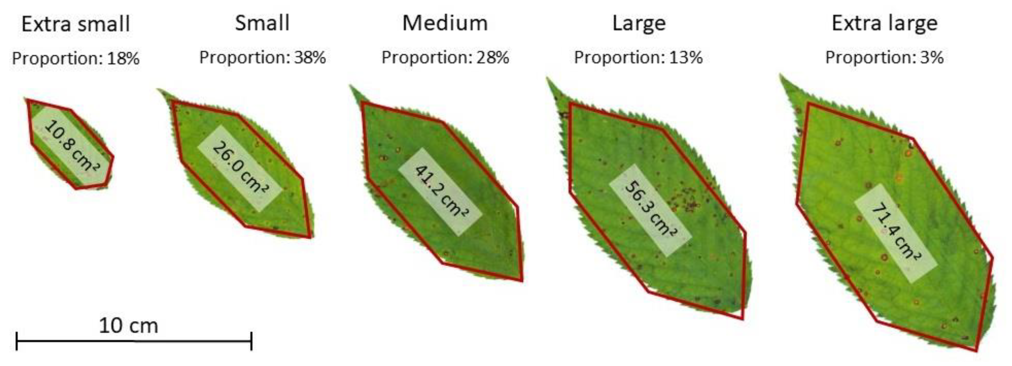
To gain insights in leaf patterns (i.e., shape distribution, size distribution, and spatial distribution within-trees), we sampled 58 branches from eight cherry trees growing in analogous conditions as the six laser-scanned trees. Branches were randomly selected from different tree heights, starting from the crown base to the tree top, and in multiple cardinal directions. We cut these branches at the branch collar, manually removed their leaves, and stored them in separate bins, which were weighed. A subset of 20 branches has been photographed with a scale to determine branch parameters, such as branch collar diameter, branch length and branch specific mass. From the leaf bins, 630 fresh leaves were randomly drawn and scanned with a ScanMaker 9800XL plus (Microtek International, Inc.; Hsinchu City, Taiwan) in a resolution of 600 dpi, to gather information of the leaf dimensions with the software ImageProPlus Version 7.0.1 (Media Cybernetics, Inc.; Rockville, MD, USA). Leaf length, leaf width and leaf area (one-sided area of the leaf blade) were measured. We divided the leaf area observations into five sets of equal length, every 15.1 cm² apart from minimum to maximum values (Figure S1). In addition, we determined the leaf area distribution, defined five leaf size classes by taking the mean leaf area of each range (extra small, small, medium, large, extra-large) and obtained their proportions, as shown in Figure 3. Lastly, we computed hexagonal leaf-like shapes with the geometric parameters derived from leaf measurements.
The realistic leaves were initially designed as regular six-sided polygons. We calculated leaf length and leaf width for the leaf classes by averaging minimum and maximum values for each leaf in the scanning procedure. Hence, the average lower leaf edges were at 38% of the leaf length, while the average upper leaf edges at 68%. Both lower and upper edges were placed equidistant within the minimum diameter. The area of the convex hull of the six points was calculated as leaf area. Finally, the geometric edges were adjusted by a ratio, so that the mean leaf, representative of a size class, keeps the corresponding average leaf area (Table S1). The resulting irregular hexagons can be seen in Figure 3. The final realistic leaves representatives of the five classes were defined by six geometric points (Table S2). Leaf geometry, area, length and width, as well as insights on the distribution and proportion of leaves, were used to feed the leaf creation algorithm (LCA).
The LCA was developed to overlay realistic leaves on the top of a QSM generated with TreeQSM. The distribution of leaves follows the pre-set information on leaf geometry and leaf size classes proportion, the 3D tree-cylinder model properties and the user-defined input parameter “leaf spacing”. On a tree basis, for a range of virtually created leaves with increasing leaf spacing (0.5, 1.0, 1.5, 2.0, 2.5, and 4.0 cm), preliminary results [52] revealed the leaf spacing of 2 cm being the most suitable to match the estimated total leaf area in first order branches (mean percentual overestimation of 7%; Figures S2 and S3). The algorithm outputs consist of two data frames: the leaf edge coordinates dataset (six points defining leaf geometry and orientation), in a coordinate system respective to the input QSM, and; an informational table containing leaf attributes (leaf number, size class, area, origin).
The steps imbedded in the LCA are described in Algorithm 1. First order branches assumed a central role in the leaf generation process, while stem-cylinders were prohibited from receiving leaves. According to the insights obtained on leaf distribution and from the starting position of a first order branch, branch-cylinders were foliated if distanced in magnitude equal or greater to 8.47 % of the length of the respective first order branch (Figure S4). Selected branch-cylinders were given leaf positions according to leaf spacing and an alternate distichous phyllotaxy (right and left arrangement). A virtual petiole (the stalk that attaches the leaf blade to the branches) of 2 cm was set from the initial leaf position. Furthermore, a random leaf area class was selected and the leaf-bottom point was matched with the extended leaf position. The other five leaf-geometry points were calculated by keeping leaf azimuth angle perpendicular to the cylinder direction (left or right direction) and leaf blade parallel to the ground plane. The six leaf-geometry points were presented in XYZ coordinates relative to the input QSM. The leaf edge coordinates output dataset was used as input within the shadow model, jointly with the tree-cylinder model.
Algorithm 1 Leaf Creation Algorithm (LCA)
1:Load a tree-cylinder model (QSM)
2:Define parameter leaf spacing (i.e., 2 cm)
3:for each first order branch do
4:  define branch section to be foliated (e.g., the first 8.47% of the length of a first order branch have no leaves).
5:  for each branch cylinder to be foliated do
6:   Establish positions for leaves along the directional axis between cylinder start and end, according to the parameter leaf spacing, and evenly distribute them, alternating between left and right side.
7:   Expand the preliminary leaf position with 2 cm (adding a virtual petiole), perpendicular to cylinder direction and horizontal to the ground, respecting the right or left orientation (+90° or −90° from cylinder direction)
8:   for each leaf position do
9:     Randomly select a leaf-size class and match the lower leaf-geometry point with the established leaf position.
10:     Propagate the other five leaf-geometry points by keeping leaf oriented perpendicular to cylinder direction and horizontal to the ground.
11:     end for (step 8)
12:  end for (step 5)
13:end for (step 3)
14:return leaf edge coordinates dataframe and leaf attributes table
A descriptive summary of the leaves created for the shadow simulations (presented in Section 2.3) is found within Table 3. The total leaf area correlates well with branch volume and other tree properties (i.e., cumulative branch length), and varied considerably between trees. Likewise, total leaf count ranged from 12,539 (Pa_6) to 35,194 (Pa_5). The proportions of leaves found for each leaf-size class confirmed our LCA is not biased.
  • Part D: Updated Shadow Model
We refined the shadow model proposed by [32] in two major aspects: (1) we integrated the output of the LCA to simulate the shading effects of trees (QSMs with realistic leaves); and (2) we expanded the functionalities of the algorithm to be compatible with the data-frame structure and building-logic of TreeQSM (previously based on SimpleTree), including the module related to the creation of ellipsoidal leaves (EL). The updated shadow model includes the realistic leaves following the same principles of the initial method, where cylinders and ellipsoids (as leaf-replacements) are taken as structures to project shadows on the ground under a given sun position.
For simulations of the EL leaf-on mode, we modified the cylinder-radius threshold for ellipsoids, proposed by Rosskopf et al. [32], from 0.5 to 1.0 cm (algorithm parameter defining where leaf-replacements are to be built upon) and adjusted the length of the longer/major ellipsoids axis, while the minor axis was set to 5.0 cm. Apart of the size limitation, ellipsoids were created for each set of cylinders in a branch order, where the threshold applied. At the given level of implementation, a change in size to simulate leaf growth was not needed as the shade cast was modelled for the leaf attributes given in the month of July 2019.
For modelling the insolation on the ground plane, we used measured data of solar irradiance (global radiation and diffuse radiation) provided by the German Meteorological Service (DWD) [53] and chose the nearest meteorological station located in Freiburg (48°01′12.0″N 7°49′48.0″E, 236.5 m a.s.l.), about 15 km from the location of the scanned trees. The solar radiation data for July 2019, with a temporal resolution of 10 min, was integrated within the shadow model.
In summary, the updated shadow model was implemented in the open source language R, version 3.5.3 [54], and is based on key functions of the R packages “sp” [55,56] and “insol” [57]. In addition, we utilised functions of the package “rgl” [58] for visualisation purposes.

2.3. Shadow Simulations

The shading effects of trees were modelled for the period of 1 July to 31 July 2019, with three leaf modes:
  • QSMs with leaves created with the LCA (realistic leaves, RL);
  • QSMs with ellipsoids as leaf-replacements (ellipsoidal leaves; EL);
  • QSMs without leaves (no leaves; NoL): we were also interested in the effect of leaves on the shading in relation to a tree outside the vegetation period, under leaf-off conditions.
To quantify the loss of insolation due to the physical obstacles (the tree structure and leaves), we simulated the insolation for a raster grid size of one third of a hectare (70 m × 50 m), with cell size of 100 cm² (10 cm × 10 cm), and centralised on the tree’s position. Insolation was determined for each raster cell at a 10-min interval. Shaded grid cells received the actual diffuse radiation value, while global radiation values were attributed to cells under full light conditions.
In order to compare shadow model results, we simulated insolation with an alternative established method named hemispherical photography (HP). We took photos of the same wild cherry trees in leaf-on conditions in July 2018 using a Canon EOS 700D camera (Canon Inc.; Tokyo, Japan) with a Sigma 4.5 mm F2.8 EX DC HSM Circular Fisheye objective (Sigma Corp.; Kawasaki, Japan). Photos were taken every 2 m on a transect originating at the base of the tree to a distance of 10–14 m. The symmetric growth of the open-grown trees made it possible to take the pictures in one cardinal direction and apply the derived photographs to the remaining eight transect lines. The subsequent hemispherical photographs were first processed to produce a black and white binarized image and then analysed using HemiView Version 2.1 software (Delta-T Devices Ltd.; Cambridge, England) to derive values for global, diffuse, and indirect site factors for each photograph position in the transect in relation to cardinal direction and the position of the sun in the sky throughout the month of July 2019. Basic settings were used including the “Default Simple Model” as solar model, an evenly split ratio (50:50) of the direct and indirect site factor, suggested by Canham et al. [59] as a typical value for the distribution of solar radiation under open area conditions for the sample site’s latitude. To ease the comparison, the HemiView output shadow was interpolated to the same grid cell size as the output of our shadow model, a square with sides each of 10 cm.

2.4. Comparisons and Analysis of Shading Effects

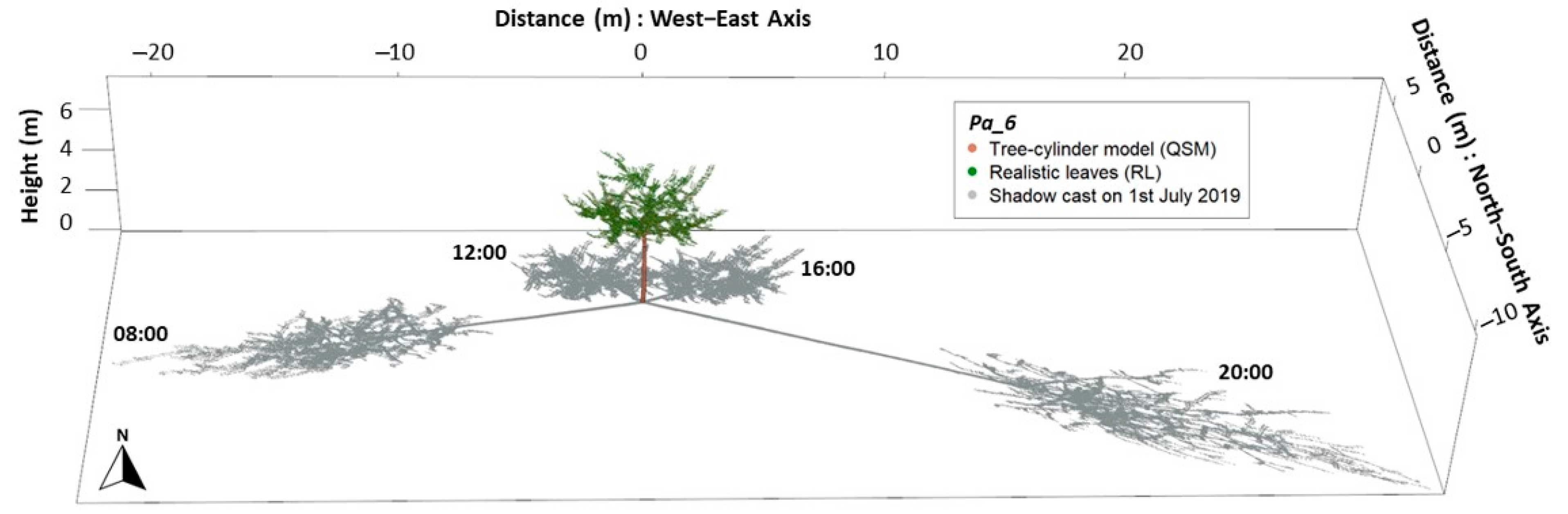
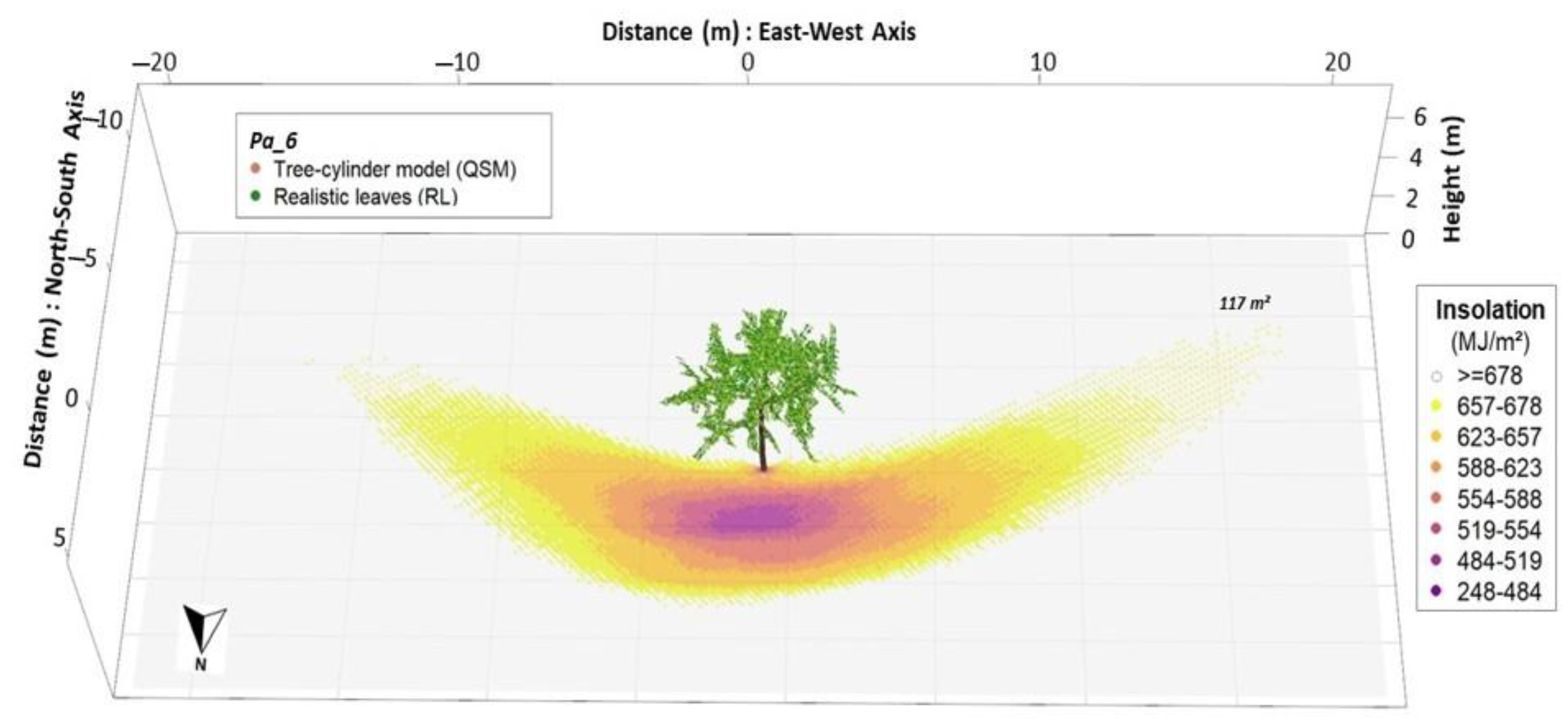
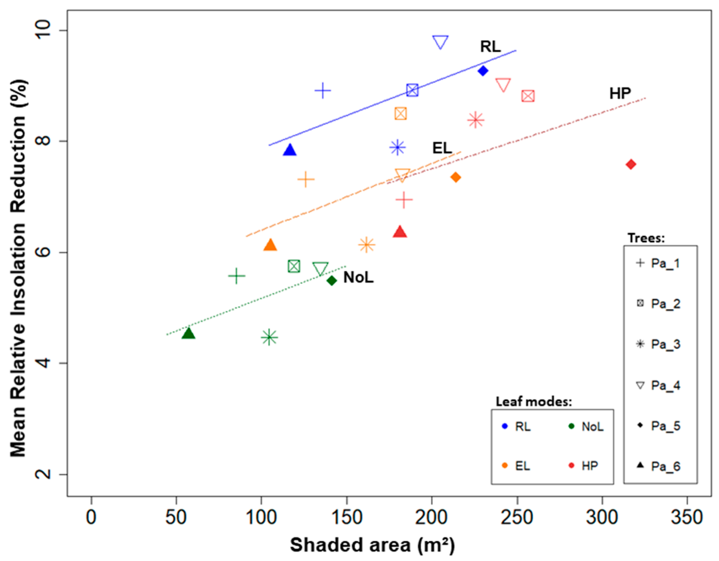
We explored the heterogeneity of the modelled shading effects in terms of monthly insolation, and compared it to full radiation conditions to estimate the shading effect: the total shaded area, and the absolute and relative insolation reduction.
The shaded area was defined as the area sum of grid cell receiving less than 98% of the maximum possible insolation (cells with insolation reduction), whereas the remaining cells were defined under full light conditions (no decrease in insolation). On each shaded area, total insolation reduction was calculated as the sum of differences between the maximum radiant energy potentially available on a grid cell and the actual radiant energy found on it. Furthermore, we investigated the shaded area proportion under different shade intensities (in percent), as defined:
s h a d e   i n t e n s i t y   ( % ) = ( 1 x 1 x 2 ) 100
where
x1 = sum of 10-min incoming radiation energy per grid cell over simulation period (31 days), under possible shaded conditions (insolation <98% of the maximum possible insolation);
x2 = sum of 10-min incoming radiation energy per grid cell over simulation period (31 days), under full light conditions (insolation ≥98% of the maximum possible insolation).
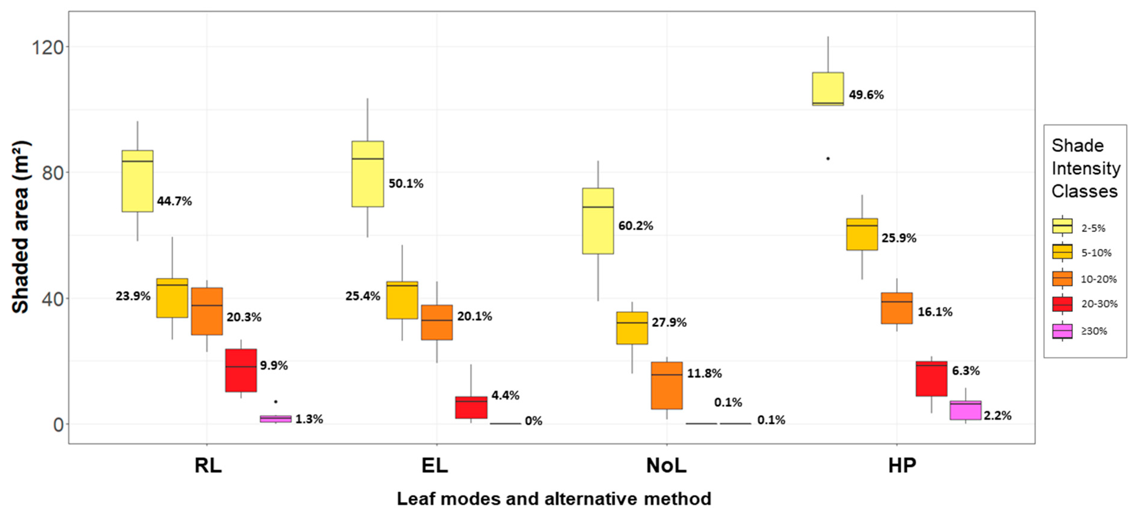
Shade intensity values were split in classes of relative insolation reduction, as the intensity of shading have varied effects on the establishment and productivity of agricultural crops [9]. The five shade intensity classes were 2–5%; 5–10%; 10–20%; 20–30%; and >30% insolation reduction. We calculated the results for each tree under each of the four treatments (RL, EL, NoL, and HP). Lastly, we investigated the spatial heterogeneity for pairs of observations taking RL as references (RL against EL, NoL and HP).
In order to parameterise the bivariate spatial dependence, and to test the similarity of the spatial patterns of the shading effects, we calculated the bivariate association measure L [60,61]. For these spatial analyses, we used a subset data corresponding to a grid area of 128 m² (rectangle of 16 m × 8 m), encompassing the majority of the insolation reduction on ground, from the tree trunk 2 m to the south, 6 m to the north, and 8 m towards west and east directions.
The L measure, the univariate spatial association measures (SSSx and SSSy) and correlation coefficients associated to it, were estimated with the “spdep” library [55] in the R environment v 3.5.3 [54]. For the insolation reduction grid data, neighbours were created with the “cell2nb” function and the type of sharing boundary connectivity was set to “queen”; weights were given with the “nb2listw” function, and the globally standardised coding scheme style (“C”) was chosen [62]. A permutation test for the L measure (400 random permutations, “lee.mc” function) of x and y (RL and EL, NoL or HP shading effects, respectively) for the given spatial weighting scheme established the rank of the observed statistic and calculated “pseudo p-values”.

3. Results

We modelled the shade cast based on QSMs of six wild cherry trees for July 2019, at 10 min intervals, retrieved and compared the shading effects in the ground for the leaf modes (RL, EL, and NoL) and HP.

3.1. Modelling Insolation and Shading Effect with RL

Using our approach to simulate tree canopy with realistic leaves (RL), we modelled the insolation reduction for six wild cherry trees. In Figure 4, the shade cast by tree Pa_6 with RL is displayed for four timestamps (at 08:00, 12:00, 16:00, and 20:00 real local time; CEST) for 1 July 2019. In addition to the differing orientation of the shadow projections, the size and extent for the different daytimes can be observed. According to the sun movement for the northern hemisphere, the shadow projection is moving clockwise starting in a south-westerly direction early in the early morning and ending closer to the south-east direction in the nightfall. From the base of the tree, the projected shadow length was: 20 m towards the west, at the beginning of the day; 6 m towards the north, at midday and early afternoon; and 30 m to the east, prior to sunset. The number of active sun positions for the simulation period of July was 2865 (a total of 477.5 h of sunlight), meaning that the same number of shadow projections were modelled, for the six trees under different leaf modes, to estimate the shading effects: monthly insolation, insolation reduction, and shaded area.
For the simulation period of July 2019, the maximum insolation was 691.98 MJ m−2, or 22.32 MJ m−2 day−1, on a daily basis. In Figure 5, the insolation around tree Pa_6 with RL is shown: the darker the colours, the greater the shading effect. Likewise, it is possible to observe areas of more intense energy reduction. For Pa_6, the mean insolation was 637.95 MJ m−2, while the mean insolation reduction was 54.0 MJ m2.
In all trees with RL, the spatial distribution of the shading effect had a hyperbolic shape around the trees, with the strongest insolation reduction towards the north direction at a distance of ±7 m to the tree trunk. It spread roughly 16 m to the east and west direction, 8 m to the north and 4 m towards south-west and south-east. We found no shading effects towards the south. In addition, the mean insolation reduction was 60.7 MJ m−2 (±5.4) for RL, while the average shaded area was 175.91 m² (±42.56) per tree. On a daily basis, this resulted in an insolation reduction of 1.96 MJ m−2 day−1 (±0.17).

3.2. Model Comparison

We investigated the shading effects of all trees and leaf modes. Monthly insolation correlated strongly with the shaded area (~0.99), meaning the larger the shadows, the greater the shading effects. For all leaf modes, total monthly insolation ranged from 37,777.8 MJ (Pa_6 NoL) to 144,360.7 MJ (Pa_4 RL), and the total insolation reduction varied between 1782.7 MJ (Pa_6 NoL) and 14,753.2 MJ (Pa_4 RL). Furthermore, the shaded areas were greater for RL, and varied greatly within trees and leaf modes: from 57.17 m² (Pa_6 NoL) to 229.94 m² (Pa_5 RL).
The mean shading effects are presented in Table 4. Shaded area for HP were greater in size compared to the QSM-based leaf modes. The respective minimum and maximum shaded areas were: 181.15 m² (Pa_6 HP), and; 316.93 m² (Pa_5 HP).
The shading effects of each tree and treatments is exemplified in Figure 6: the shaded area in comparison with the mean relative insolation reduction (colours specify the simulation set and symbols represent the sample trees). An effect of the differing leaf modes on the relative insolation reduction can be observed. RL showed more intense shading effects compared to concurrent modes, with a mean relative insolation reduction of 8.77% (±0.78). The mean relative insolation reduction in ascending order was: NoL < EL < HP < RL. The shading effect on a tree basis can be seen in Table S3.
The shaded area and mean proportion of each shade intensity classes can be observed in Figure 7. Over all simulations, we found a predominant shading effect in the two lowest intensity classes: 51.1% of shaded area are covered by the first class (2–5%), and 25.8% by the second class (5–10%). For RL, it was found an increased proportion of shaded area under the shade intensity classes 20–30% (9.9%) and ≥30% (1.3%), compared to EL and NoL. The portion of shaded area under 10–20% insolation reduction was similar between RL and EL, 20.3% and 20.1%, respectively. The shading effects of HP had a particular pattern: they varied in content for all intensity classes, and their proportions were more evenly distributed between classes with a negative exponential trend.
The spatial distributions of EL and NoL shading effects were similar to RL: a hyperbolic shape around trees towards the north, where the strongest shading effect is manifested; with shade-free zone towards the south. However, they had reduced dimensions on the east-west and north-south axis compared to RL.
Hemispherical photography shadows spread differently. Shaded area was more regularly distributed around the tree trunk position (at 0,0,0), in a circular fashion, with a varying radius of 8 m to 14 m. For all trees, a more intense insolation reduction effect was found within the first 4 m around tree stem and directed to the north (similarly to the QSM-based shadows). Compared to RL, the shaded area had a shorter range in the east and west directions and, surprisingly, a strong insolation reduction around 4 m towards south.
The modelled insolation reduction is shown in Figure 8 for trees Pa_4 and Pa_6: the shading effects are zoomed to details limited at 8 m around tree trunk and presented in blocks comparing simulation sets. We observed areas of greater shading intensity on the shaded area (see Pa_4 with RL), which may correspond to branches of outstanding size, higher branchiness and/or higher leaf density in certain parts of the tree canopy.
Within the subset area focused on the insolation reduction of RL mode, we investigated the aggregation and similarity of the shadows in terms of spatial and aspatial association measures. All measures are reported in Table 5, and key measures are displayed in Figure 8.
Values for the spatial smoothing scalars SSSx and SSSy confirmed that shading effects are spatially clustered. Often the clustering effect was stronger in EL than in RL, as ellipsoids project longer and more uniform fractions of shadow to the ground than RL, producing more similar neighbouring values on the ground. These measures of univariate spatial association offer a reference point (roof value) for the interpretation of the bivariate spatial association measure L.
For all trees, RL shading effects correlated strongly with EL (0.98–0.99), less strongly with NoL (0.89–0.95), and moderately with HP (0.55–0.80). The global L measure presented similar trend for the paired comparison of spatial distribution of shadows (RL shadows versus other modalities), which revealed a strong spatial similarity of the shading patterns RL-EL, and RL-NoL, and dissimilarity of RL-HP. Moreover, L statistic worked as a superior alternative to Pearson’s correlation coefficient, as it captured the magnitude of the spatially clustering of the bivariate spatial associations [63].
The permutation test showed that all paired shading effects were spatially autocorrelated (pseudo p-value of 0.0025 unanimous; rank 400 of 400 simulations), and we therefore, accepted the alternative hypothesis that there is a greater variability in the shadows, which are not explained by the similarities of the spatial pattern of the insolation reduction area. In the case of leaf modes, this is an evidence that the leaf pattern has an effect on the shading effects, since the woody structure defined by the QSM did not vary.

4. Discussion

The presented LCA and updated shadow model constitute a refined approach for the use of QSMs of real trees augmented with realistic leaves (as mean of canopy reconstruction) for modelling tree shading effects on the tree surroundings in high temporal and spatial resolution.

4.1. Leaf Creation Algorithm in Comparison to Others

To date several researchers have worked towards estimating tree and forest structural attributes and foliage properties from TLS point clouds. Côté et al. [64] worked with needle modelling for four conifer species to define the total amount of foliage in the crown and build the tree branching structure. Zheng and Moskal [65], presented a new method that indirectly and non-destructively retrieves foliage elements from TLS point clouds, assuming that tree leaf orientation, is an important attribute of forest canopy architecture and is critical in determining the within and below canopy solar radiation regimes. The separation of foliage and wood in TLS points clouds has been studied by many [28,50,66]. In all these studies the research goals have been diffuse, in cases towards reconstructing perfectly the woody architecture of trees or simply for deriving leaf attributes and insights on the light regime. Åkerblom et al. [42] presented a non-intersecting leaf insertion algorithm for tree structure models, its open MATLAB implementation, and conducted initial testing for English Oak (Querus robur L.). Similarly, to our LCA, the algorithm implementation is a tool aiming for realistic canopy reconstruction of trees and allows users to set the leaf shape (triangle-based geometry like) and distribution of leaf location, size and angles.
Many different parameters can be used to define leaf distribution on a tree to fully reconstruct canopy architecture. In this context, the LCA was designed for a simplified approach having few assumptions embedded, and parameters set to constant values: leaf inclination angle is 0°, parallel to a theoretical horizontal ground plane; phyllotaxy is defined as alternate distichous, which delivers leaves arranged alternatively to the left and right on a same plane; leaf orientation is +90° or −90° (right or left) apart of the specific branch-cylinder directional axis; leaf disposition on the branch is ruled by the allometric relationship, establishing a leafless zone for first order branches. A main concern with the leaf inclination angle is that steeper angles decrease light captured when the sun is at high viewpoints in the sky (midday and summer), whilst increasing light captured from lower sun angles in the morning and afternoon, as well as in winter [67]. Moreover, we do not account for leaves that are clumped together, which is observed in many wild cherry individuals. All these aspects could be source of uncertainty when modelling shade cast by trees. The only user-defined parameter is the leaf spacing, which is used for controlling the total leaf area of a tree. The allometric equation for specifying the expected leaf area on a tree was based on the measurements of thirteen branches. As a limited dataset, the total leaf area equation does not account for complex branch structures (i.e., wind-damaged branches or from pruning treatments), and a more detailed and increased sampling size would be beneficial. Although all wild cherry trees include in this study belonged to AFS, our laser-sampled trees could have received different silvicultural treatments and were exposed to diverse growing conditions (i.e., in more open landscapes, isolated trees), than the trees utilised for the manual leaf sampling. Our sample trees had total leaf area values similar to the findings of Urban et al. [68] for P. serotina with comparable DBH and height ranges. Likewise, Miljković et al. [69] presented corresponding data on leaf area, leaf width, leaf length, and petiole length of P. avium individuals from five different natural populations in Bosnia and Herzegovina.
Another source of uncertainty is the tree reconstruction with QSMs, which was controlled by the specific optimisation process inside TreeQSM, testing many model parameters over repeated model runs [41]. In addition, the parameter “cylinder length” could play a major role in the EL leaf mode, as the construction of the ellipsoidal leaves is determined by the branch-cylinder diameter (i.e., 1 cm), so that an increased number of cylinders per branch is preferred.
Even if we used specific plants traits for model parameterisation and for defining assumptions, this could still be further adapted to any tree species by changing specific algorithm parts to user-defined options and values. An alternative to parameterise the leaf inclination angle would be by using the dataset provided by Chianucci et al. [70], which offers species-specific parameters and cover a great range of broadleaved tree and shrub species in temperate and boreal regions. Dataset observations are derived with the established levelled digital photography (LDP) approach, which is known of sensing only leaves oriented approximately parallel to the viewing direction of the camera, and are restricted to the source locations (Sweden, Estonia, USA, central Italy). Furthermore, LiDAR based approaches for assessing leaf angle distribution already overcame some of the shortcomings of LDP as they are not limited by leaf curvature [71], and might be a new data source for parameterisation of the LCA.

4.2. Shadow Simulations—Performance and Comparison

A full investigation of interrelations of QSM-derived tree parameters and shading effects was beyond the scope of this study. Nevertheless, we noticed greater shading effects with an increased tree structure (e.g., branch volume), the case for Pa_4 and Pa_5. Conventionally, tree height and crown size and density are noticeably affecting the shaded area and intensity of the shading effect. There was a trend associated with the insolation reduction which was clearly an effect of the leaf mode on a per tree basis, as the tree structure (QSM) of each individual was the same. We demonstrated the reduction of insolation on different leaf modes (RL, EL, and NoL) in the comparative blocks. For all shading effects modelled by means of the shadow algorithm, the visualised heterogeneity was the true effect of leaves (RL or EL).
Hemispherical photography is a 2D approach, for this reason the comparison with highly detailed 3D point cloud data is biased. In practice, using the hemispherical photography methodology a short tree with a dense crown in a photograph could be comparable to a tall tree with a lighter crown. Photographs taken in different distances to the tree, as carried out in this study, improve the situation, but it is still less precise than 3D data. As expected, we demonstrated that hemispherical photography reports different shading effect (intensity and size) and spatial distribution than simulations with our shadow model. Within this study, we used factual weather data, corresponding to the time-period for the simulations, for RL (EL and NoL), while HP is based on average data which may suppress extreme values from July 2019 as applied to the simulations, possibly leading to differences in the shading effect of HP.
Dupraz and Liagre [20] presented examples of temporal shade cast by trees in France, their results displayed similar spatial distribution than our modelled shadows, but lacked the important fine spatial resolution. This approach of modelling the radiation regime around trees based on 3D structures used a replacement of the complete tree crown by an ellipsoid for modelling the light availability in AFS. The method was further developed by Talbot and Dupraz [21], which proved the efficiency of the model to predict the light pattern around an average tree, but not suitable for simulating the variability of individual trees.
It was observed that the shadows modelled with RL had a greater shading effect compared to the adjusted ellipsoidal leaf-replacement proposed by Rosskopf et al. [32]; unsurprisingly, RL and EL distributed similarly on space, and the shading effect of EL was often more clustered than RL. EL is a simplified leaf mode and is species independent. An additional calibration of the cylinder-radius threshold for the suggested ellipsoids (i.e., greater than 1.0 cm) could improve the results of EL in this study. It was noted that spherical-like leaf structures were formed with the EL approach, as well as few ellipsoids of distinguished length. On a specific branch order, single branch-cylinders with radius ≤ 1.0 cm, or a short set of cylinders, produced and ellipsoidal leaf akin to a sphere, or a coin shape. The extremely large ellipsoids are associated to the branch order of a branch ramification, and/or the uncertainty of the QSM. In the first case, where branch-cylinder radius were ≤ 1.0 cm, the lowest branch order could have had a large total length, and consequently a noticeably large ellipsoidal leaf. Secondly, due to noise or occlusion in the tree point clouds, unrealistic branch ramification could have been produced within the QSMs, which led to the creation of few ellipsoids of outstanding length. Though EL could be applied openly for any tree species, it is case-sensitive, since plant traits (i.e., leaf traits), tree architecture and reconstruction with QSMs are likely to influence the choice of the optimal parameters’ values, what also justifies the optimisation of QSMs (conducted in this study).
The RL scenario assumption of horizontal leaf angle could have slightly overestimated the shading effects during the summer period (shaded area, and thus, a reduction of insolation). In reality, such leaf orientation is different to the simplified rules applied herein. Leaves could have a focal point on the sun’s sky path, being horizontal when shaded or with varied angles to the incoming sunlight [72]. Moreover, leaves could be sparser, but bigger on the northern side to ensure adequate light interception [73]. Further efforts must be devoted to improve simulations and models based on the orientation of leaf planer surfaces affixed to the QSM. Represented by NoL, the leaf-off condition of trees remains relevant for AFS, since crops such as winter wheat could benefit from broadleaved trees without leaves in late autumn and winter and may be disproportionally impacted by shade cast due to reduced insolation at this time of year. NoL had reliable results as the spatial distribution of the shadows is very similar to the RL (in the focused shaded area), however, the shading effect is reduced to approximately 40% (area and intensity) in relative terms. This information could be used to simplify our approach, as adding leaves is time consuming, shadows produced with QSMs (alone) could already give precise location and a rough estimation of the shaded area and insolation reduction over a time period, possibly correcting it with an expansion factor.
Shadow simulations and comparisons of shading effect of leaf modes were carried out only for July, and these results agreed with the general spatial pattern presented by Rosskopf et al. [32]. Therefore, we would expect similar results independent of the month of the year.
Finally, we acknowledge a few limitations of our approach. Our shadow algorithm, implemented in R environment, requires high computational power for the leaf-on modes (≥32 Gb RAM, in many cases) and is still time consuming (~52 h of simulations for one tree, at the highest spatial and temporal resolution for one month). Simulations for the leaf-off mode were faster (~16 h). While a full assessment of algorithm performance was not targeted within this study, we recognise the need for further algorithm improvement and efficiency optimisation. Up to now, the shadow model does not have an openly available implementation. Once accessible, a fully standardised implementation of the shadow model should consider a standard way of delivering outputs, including analytical simulation reports. First-hand laser data obtained with TLS remains costly and inaccessible for many research groups around the word. In contrast, point clouds of forest stands and trees, as well as QSMs, are becoming increasingly available, enabling users to search for 3D data to be applied with the scope of modelling shading effects. The use of specific weather data makes the simulations of insolation case-specific, but for an open adoption of our method, it could offer a standardised protocol for including any region on earth. A full validation of the shadow model will require more efforts at field level and would have to include a thorough assessment for calibrating model parameters; such a solution is sought in the visible future.

5. Conclusions

We presented an updated shadow model that uses factual 3D data in combination with a leaf creation algorithm (LCA) to estimate individually the shading effect of six wild cherry trees growing under agroforestry conditions in southern Germany. The coupling of the shadow model with factual climate data added to the accuracy of the model. This approach was able to refine simulations of the shading effects of scattered trees represented by QSMs with realistic leaves (RL). We also evaluated the shading effects of other leaf moves (EL and NoL). As a simplified leaf-on mode, EL had similar distribution of the shading effect with slight underestimation in total insolation reduction and shaded area. Though RL might be closer to reality, the EL mode could be an alternative for the (at the time) exhaustive time consumption of simulations with RL. Likewise, the shading effects of NoL leaf-off mode were also similarly distributed to RL, though reduced by almost half of the intensity. The shading effects of NoL gave us insights on the potential of leafless woody structures to act as obstacles mediating the radiation regime on ground. The alternative method had dissimilar shading effects and distribution.
The shadow model is a suitable tool for the detailed quantification of the shading effects of single trees. We estimated insolation reduction and shaded area values focused on the particularities of the tree structures. Our approached is limited to work with QSMs, what implies in sample trees to be scanned outside the vegetation period. Derived results can be utilised to support decision-making by land managers, in agricultural and agroforestry systems, or even to facilitate the inclusion of trees in urban areas, as a strategic public health measure.

6. Outlook

We fulfilled our aim of developing an improved simulation of the shading effects of single-trees, but further improvements of the shadow model are foreseen. First, increasing algorithm capabilities for handling data from multiple trees [74]. Secondly, enabling the leaf inclination angle to be set as an input parameter and/or to follow a distribution function. Moreover, increasing capabilities to address phyllotaxy and leaf geometry of other tree species. Lastly, the inclusion of growth simulations to account for the growth of the trees during the vegetation period.

Supplementary Materials

The following are available online at https://0-www-mdpi-com.brum.beds.ac.uk/2072-4292/13/3/532/s1, Figure S1: Leaf area count of the five leaf size classes (extra small, small, medium, large, extra-large), establishing the proportions of leaves to be created by the Leaf Creation Algorithm (LCA). Figure S2: Linear trend between branch length and first order branch diameter (N = 12). Figure S3: Branch leaf area as a function of first order branch diameter (N = 13). Figure S4: Relative leaf area according the relative branch position. Equation root at 8.47% relative branch position defined the initial position for insertion of leaves. Table S1: Measured and adjusted leaf parameters per leaf class. Table S2: Leaf attributes that define the leaf geometry points, from which six geometric points are derived: length, width, lower and upper edges. Table S3: Shaded area and insolation reduction of wild cherry trees (Pa_1 to Pa_6, in symbols) for different leaf modes (RL, EL, and NoL) and HP. Video S1: Wild cherry tree Pa_5 reconstructed as a QSM and augmented with the leaf modes; profile and top views.

Author Contributions

R.B.R., E.L. and C.M. conceived and designed the study; E.L. and C.M. collected the field data; E.L. sketched the LCA algorithm; R.B.R. enhanced and implemented the LCA and the shadow model; R.B.R. processed and analysed the data; R.B.R., E.L., C.M., J.P.S. and H.-P.K. wrote and reviewed the publication. All authors have read and agreed to the published version of the manuscript.

Funding

This research was supported by the German Federal Ministry of Food and Agriculture (BMEL) within the SidaTim project (support code 2815ERA04C) and the German Federal Ministry of Education and Research (BMBF) within the ASAP project (grant number 01LL1803A). The article processing charge was funded by the Baden-Württemberg Ministry of Science, Research and Art and the University of Freiburg in the funding programme Open Access Publishing.

Data Availability Statement

The datasets generated during and/or analysed during the current study are available from the corresponding author on reasonable request.

Acknowledgments

We would like to thank Michael Nahm for his valuable support. Furthermore, we thank the anonymous reviewers whose comments and constructive criticism helped improve and clarify this manuscript.

Conflicts of Interest

The authors declare no conflict of interest. The founding sponsors neither had a role in the design of the study; the data collection process, the analyses, the interpretation of data; the writing of the manuscript, nor in the decision to publish the results.

References

  1. Jones, C.G.; Lawton, J.H.; Shachak, M. Positive and negative effects of organisms as physical ecosystem engineers. Ecology 1997, 78, 1946–1957. [Google Scholar] [CrossRef]
  2. Valladares, F.; Laanisto, L.; Niinemets, Ü.; Zavala, M.A. Shedding light on shade: Ecological perspectives of understorey plant life. Plant Ecol. Divers. 2016, 9, 237–251. [Google Scholar] [CrossRef] [Green Version]
  3. Sheppard, J.P.; Bohn Reckziegel, R.; Borrass, L.; Chirwa, P.W.; Cuaranhua, C.J.; Hassler, S.K.; Hoffmeister, S.; Kestel, F.; Maier, R.; Mälicke, M.; et al. Agroforestry: An Appropriate and Sustainable Response to a Changing Climate in Southern Africa? Sustainability 2020, 12, 6796. [Google Scholar] [CrossRef]
  4. Nair, P.K.R. Classification of agroforestry systems. Agroforest. Syst. 1985, 3, 97–128. [Google Scholar] [CrossRef]
  5. Leakey, R. Definition of agroforestry revisited. Agrofor. Today 1996, 8, 5. [Google Scholar]
  6. Editors of Agroforestry Systems. What is Agroforestry? Agroforest. Syst. 1982, 1, 7–12. [Google Scholar] [CrossRef]
  7. Eichhorn, M.; Paris, P.; Herzog, F.; Incoll, L.; Liagre, F.; Mantzanas, K.; Mayus, M.; Moreno, G.; Papanastasis, V.; Pilbeam, D.; et al. Silvoarable Systems in Europe–Past, Present and Future Prospects. Agroforest. Syst. 2006, 67, 29–50. [Google Scholar] [CrossRef]
  8. Blaser, W.J.; Oppong, J.; Yeboah, E.; Six, J. Shade trees have limited benefits for soil fertility in cocoa agroforests. Agric. Ecosyst. Environ. 2017, 243, 83–91. [Google Scholar] [CrossRef] [Green Version]
  9. Schulz, V.S.; Munz, S.; Stolzenburg, K.; Hartung, J.; Weisenburger, S.; Graeff-Hönninger, S. Impact of different shading levels on growth, yield and quality of potato (Solanum tuberosum L.). Agronomy 2019, 9, 330. [Google Scholar] [CrossRef] [Green Version]
  10. Landsberg, J.J.; Sands, P.J.; Landsberg, J.; Sands, P. Physiological Ecology of Forest Production: Principles, Processes and Models; Elsevier/Academic Press: Amsterdam, The Netherlands, 2011. [Google Scholar]
  11. Monteith, J.; Unsworth, M. Principles of Environmental Physics: Plants, Animals, and the Atmosphere; Academic Press: Cambridge, MA, USA, 2013; ISBN 0123869935. [Google Scholar]
  12. Cutini, A.; Matteucci, G.; Mugnozza, G.S. Estimation of leaf area index with the Li-Cor LAI 2000 in deciduous forests. For. Ecol. Manag. 1998, 105, 55–65. [Google Scholar] [CrossRef]
  13. Hill, R. A lens for whole sky photographs. Q. J. R. Meteorol. Soc. 1924, 50, 227–235. [Google Scholar] [CrossRef]
  14. Evans, G.C.; Coombe, D.E. Hemisperical and Woodland Canopy Photography and the Light Climate. J. Ecol. 1959, 47, 103–113. [Google Scholar] [CrossRef]
  15. Chazdon, R.L.; Field, C.B. Photographic estimation of photosynthetically active radiation: Evaluation of a computerized technique. Oecologia 1987, 73, 525–532. [Google Scholar] [CrossRef]
  16. Rich, P.M.; Clark, D.B.; Clark, D.A.; Oberbauer, S.F. Long-term study of solar radiation regimes in a tropical wet forest using quantum sensors and hemispherical photography. Agric. For. Meteorol. 1993, 65, 107–127. [Google Scholar] [CrossRef]
  17. Roxburgh, J.R.; Kelly, D. Uses and limitations of hemispherical photography for estimating forest light environments. N. Z. J. Ecol. 1995, 19, 213–217. [Google Scholar]
  18. Comeau, P.G.; Gendron, F.; Letchford, T. A comparison of several methods for estimating light under a paper birch mixedwood stand. Can. J. For. Res. 1998, 28, 1843–1850. [Google Scholar] [CrossRef]
  19. Bellow, J.; Nair, P.K.R. Comparing common methods for assessing understory light availability in shaded-perennial agroforestry systems. Agric. For. Meteorol. 2003, 114, 197–211. [Google Scholar] [CrossRef]
  20. Dupraz, C.; Liagre, F. Agroforesterie: Des Arbres et des Cultures, 2nd ed.; Éditions France Agricole: Paris, France, 2011. [Google Scholar]
  21. Talbot, G.; Dupraz, C. Simple models for light competition within agroforestry discontinuous tree stands: Are leaf clumpiness and light interception by woody parts relevant factors? Agroforest. Syst. 2012, 84, 101–116. [Google Scholar] [CrossRef]
  22. Stadt, K.J.; Lieffers, V.J. MIXLIGHT: A flexible light transmission model for mixed-species forest stands. Agric. For. Meteorol. 2000, 102, 235–252. [Google Scholar] [CrossRef]
  23. Zhao, W.; Qualls, R.J.; Berliner, P.R. Modeling of the short wave radiation distribution in an agroforestry system. Agric. For. Meteorol. 2003, 118, 185–206. [Google Scholar] [CrossRef]
  24. Sinoquet, H.; Sonohat, G.; Phattaralerphong, J.; Godin, C. Foliage randomness and light interception in 3-D digitized trees: An analysis from multiscale discretization of the canopy. Plant Cell Environ. 2005, 28, 1158–1170. [Google Scholar] [CrossRef]
  25. Sinoquet, H.; Stephan, J.; Sonohat, G.; Lauri, P.É.; Monney, P. Simple equations to estimate light interception by isolated trees from canopy structure features: Assessment with three-dimensional digitized apple trees. New Phytol. 2007, 175, 94–106. [Google Scholar] [CrossRef] [PubMed]
  26. Schmidt, M.; Nendel, C.; Funk, R.; Mitchell, M.G.E.; Lischeid, G. Modeling Yields Response to Shading in the Field-to-Forest Transition Zones in Heterogeneous Landscapes. Agriculture 2019, 9, 6. [Google Scholar] [CrossRef] [Green Version]
  27. Van der Zande, D.; Stuckens, J.; Verstraeten, W.W.; Muys, B.; Coppin, P. Assessment of Light Environment Variability in Broadleaved Forest Canopies Using Terrestrial Laser Scanning. Remote Sens. 2010, 2, 1564–1574. [Google Scholar] [CrossRef] [Green Version]
  28. Béland, M.; Widlowski, J.-L.; Fournier, R.A.; Côté, J.-F.; Verstraete, M.M. Estimating leaf area distribution in savanna trees from terrestrial LiDAR measurements. Agric. For. Meteorol. 2011, 151, 1252–1266. [Google Scholar] [CrossRef]
  29. Dauzat, J.; Madelaine-Antin, C.; Heurtebize, J.; Lavalley, C.; Vincent, G. How Much Commercial Timber in Your Plot, How Much Carbon Sequestrated in the Trees, How Much Light Available for Undercrops? Terrestrial LIDAR is the Right Technology For Addressing These Questions. In 3rd European Agroforestry Conference-Book of Abstracts; Gosme, M., Ed.; CIRAD: Montpellier, France, 2016; pp. 121–124. ISBN 978-2-87614-717-1. [Google Scholar]
  30. Cifuentes, R.; van der Zande, D.; Salas, C.; Tits, L.; Farifteh, J.; Coppin, P. Modeling 3D Canopy Structure and Transmitted PAR Using Terrestrial LiDAR. Can. J. Remote Sens. 2017, 43, 124–139. [Google Scholar] [CrossRef]
  31. Grau, E.; Durrieu, S.; Fournier, R.; Gastellu-Etchegorry, J.-P.; Yin, T. Estimation of 3D vegetation density with Terrestrial Laser Scanning data using voxels. A sensitivity analysis of influencing parameters. Remote Sens. Environ. 2017, 191, 373–388. [Google Scholar] [CrossRef]
  32. Rosskopf, E.; Morhart, C.; Nahm, M. Modelling Shadow Using 3D Tree Models in High Spatial and Temporal Resolution. Remote Sens. 2017, 9, 719. [Google Scholar] [CrossRef] [Green Version]
  33. Seidel, D.; Fleck, S.; Leuschner, C. Analyzing forest canopies with ground-based laser scanning: A comparison with hemispherical photography. Agric. For. Meteorol. 2012, 154–155, 1–8. [Google Scholar] [CrossRef]
  34. Hackenberg, J.; Morhart, C.; Sheppard, J.P.; Spiecker, H.; Disney, M. Highly Accurate Tree Models Derived from Terrestrial Laser Scan Data: A Method Description. Forests 2014, 5, 1069–1105. [Google Scholar] [CrossRef] [Green Version]
  35. Hackenberg, J.; Spiecker, H.; Calders, K.; Disney, M.; Raumonen, P. SimpleTree—An Efficient Open Source Tool to Build Tree Models from TLS Clouds. Forests 2015, 6, 4245–4294. [Google Scholar] [CrossRef]
  36. Fan, G.; Nan, L.; Chen, F.; Dong, Y.; Wang, Z.; Li, H.; Chen, D. A New Quantitative Approach to Tree Attributes Estimation Based on LiDAR Point Clouds. Remote Sens. 2020, 12, 1779. [Google Scholar] [CrossRef]
  37. Raumonen, P.; Kaasalainen, M.; Åkerblom, M.; Kaasalainen, S.; Kaartinen, H.; Vastaranta, M.; Holopainen, M.; Disney, M.; Lewis, P. Fast automatic precision tree models from terrestrial laser scanner data. Remote Sens. 2013, 5, 491–520. [Google Scholar] [CrossRef] [Green Version]
  38. Trochta, J.; Krůček, M.; Vrška, T.; Král, K. 3D Forest: An application for descriptions of three-dimensional forest structures using terrestrial LiDAR. PLoS ONE 2017, 12, e0176871. [Google Scholar] [CrossRef] [PubMed] [Green Version]
  39. Fan, G.; Nan, L.; Dong, Y.; Su, X.; Chen, F. AdQSM: A New Method for Estimating Above-Ground Biomass from TLS Point Clouds. Remote Sens. 2020, 12, 3089. [Google Scholar] [CrossRef]
  40. Raumonen, P.; Casella, E.; Calders, K.; Murphy, S.; Åkerblom, M.; Kaasalainen, M. Massive-scale tree modelling from TLS data. ISPRS Annals of the Photogrammetry. Remote Sens. Spat. Inf. Sci. 2015, 2, 189. [Google Scholar]
  41. Calders, K.; Newnham, G.; Burt, A.; Murphy, S.; Raumonen, P.; Herold, M.; Culvenor, D.; Avitabile, V.; Disney, M.; Armston, J. Nondestructive estimates of above-ground biomass using terrestrial laser scanning. Methods Ecol. Evol. 2015, 6, 198–208. [Google Scholar] [CrossRef]
  42. Åkerblom, M.; Raumonen, P.; Casella, E.; Disney, M.I.; Danson, F.M.; Gaulton, R.; Schofield, L.A.; Kaasalainen, M. Non-intersecting leaf insertion algorithm for tree structure models. Interface Focus 2018, 8, 20170045. [Google Scholar] [CrossRef]
  43. Kaasalainen, S.; Krooks, A.; Liski, J.; Raumonen, P.; Kaartinen, H.; Kaasalainen, M.; Puttonen, E.; Anttila, K.; Mäkipää, R. Change Detection of Tree Biomass with Terrestrial Laser Scanning and Quantitative Structure Modelling. Remote Sens. 2014, 6, 3906–3922. [Google Scholar] [CrossRef] [Green Version]
  44. Sheppard, J.P.; Morhart, C.; Hackenberg, J.; Spiecker, H. Terrestrial laser scanning as a tool for assessing tree growth. iForest 2017, 10, 172–179. [Google Scholar] [CrossRef]
  45. Luoma, V.; Saarinen, N.; Kankare, V.; Tanhuanpää, T.; Kaartinen, H.; Kukko, A.; Holopainen, M.; Hyyppä, J.; Vastaranta, M. Examining Changes in Stem Taper and Volume Growth with Two-Date 3D Point Clouds. Forests 2019, 10, 382. [Google Scholar] [CrossRef] [Green Version]
  46. Global Solar Atlas. GSA 2.3. World Bank Group, World. 2020. Available online: https://globalsolaratlas.info/map?c=11.523088,8.4375,3 (accessed on 3 November 2020).
  47. Morhart, C.; Sheppard, J.P.; Schuler, J.K.; Spiecker, H. Above-ground woody biomass allocation and within tree carbon and nutrient distribution of wild cherry (Prunus avium L.)—A case study. For. Ecosyst. 2016, 3, 1–15. [Google Scholar] [CrossRef] [Green Version]
  48. Pascu, I.-S.; Dobre, A.-C.; Badea, O.; Tanase, M.A. Retrieval of Forest Structural Parameters From Terrestrial Laser Scanning: A Romanian Case Study. Forests 2020, 11, 392. [Google Scholar] [CrossRef] [Green Version]
  49. CloudCompare. CloudCompare. v2.10.2 (Zephyrus) [Windows 64-bit]. 2019. Available online: http://www.cloudcompare.org/ (accessed on 4 February 2020).
  50. Disney, M.I.; Boni Vicari, M.; Burt, A.; Calders, K.; Lewis, S.L.; Raumonen, P.; Wilkes, P. Weighing trees with lasers: Advances, challenges and opportunities. Interface Focus 2018, 8. [Google Scholar] [CrossRef] [Green Version]
  51. Raumonen, P. TreeQSM. MATLAB-Software v2.30. 2017. Available online: https://github.com/InverseTampere/TreeQSM (accessed on 1 November 2018).
  52. Bohn Reckziegel, R.; Larysch, E.; Morhart, C.; Kahle, H.-P.; Seifert, T. Modelling shadow cast by trees using 3D models with artificial leaves. In Proceedings of the Book of Abstracts of the 9th International Conference on Functional-Structural Plant Models, Online, 5–9 October 2020; Kahlen, K., Chen, T.-W., Fricke, A., Stützel, H., Eds.; pp. 133–134. [Google Scholar]
  53. Deutscher Wetterdienst (DWD). CDC (Climate Data Center): Hourly Station Observations of Solar Irradiation. 2019. Available online: https://opendata.dwd.de/climate_environment/CDC/observations_germany/climate/10_minutes/solar/ (accessed on 24 February 2020).
  54. R Core Team. R: A Language and Environment for Statistical Computing. Microsoft R Open 3.5.3. Vienna, Austria, 2019. Available online: https://www.R-project.org/ (accessed on 4 February 2020).
  55. Bivand, R.S.; Pebesma, E.J.; Gómez-Rubio, V. Applied Spatial Data Analysis with R, 2nd ed.; Springer: Berlin/Heidelberg, Germany, 2013. [Google Scholar]
  56. Pebesma, E.; Bivand, R.S. S classes and methods for spatial data: Sp Package. R News 2005, 5, 9–13. [Google Scholar]
  57. Corripio, J.G. Insol: Solar Radiation. R Package Version 1.2.1. 2019. Available online: https://CRAN.R-project.org/package=insol (accessed on 4 February 2020).
  58. Adler, D.; Murdoch, D. Rgl: 3D Visualization Using OpenGL. R Package Version 0.100.19. 2019. Available online: https://CRAN.R-project.org/package=rgl (accessed on 4 February 2020).
  59. Canham, C.D.; Denslow, J.S.; Platt, W.J.; Runkle, J.R.; Spies, T.A.; White, P.S. Light regimes beneath closed canopies and tree-fall gaps in temperate and tropical forests. Can. J. For. Res. 1990, 20, 620–631. [Google Scholar] [CrossRef]
  60. Lee, S.-I. Developing a bivariate spatial association measure: An integration of Pearson′s r and Moran′s I. J. Geogr. Syst. 2001, 3, 369–385. [Google Scholar] [CrossRef]
  61. Lee, S.-I. A Generalized Significance Testing Method for Global Measures of Spatial Association: An Extension of the Mantel Test. Environ. Plan. Econ. Space 2004, 36, 1687–1703. [Google Scholar] [CrossRef] [Green Version]
  62. Tiefelsdorf, M.; Griffith, D.A.; Boots, B. A variance-stabilizing coding scheme for spatial link matrices. Environ. Plan. A 1999, 31, 165–180. [Google Scholar] [CrossRef]
  63. Kim, D.; Seo, S.; Min, S.; Simoni, Z.; Kim, S.; Kim, M. A Closer Look at the Bivariate Association between Ambient Air Pollution and Allergic Diseases: The Role of Spatial Analysis. Int. J. Environ. Res. Public. Health 2018, 15, 1625. [Google Scholar] [CrossRef] [Green Version]
  64. Côté, J.-F.; Fournier, R.A.; Egli, R. An architectural model of trees to estimate forest structural attributes using terrestrial LiDAR. Environ. Model. Softw. 2011, 26, 761–777. [Google Scholar] [CrossRef]
  65. Zheng, G.; Moskal, L.M. Leaf Orientation Retrieval from Terrestrial Laser Scanning (TLS) Data. IEEE Trans. Geosci. Remote Sens. 2012, 50, 3970–3979. [Google Scholar] [CrossRef]
  66. Ma, L.; Zheng, G.; Eitel, J.U.H.; Moskal, L.M.; He, W.; Huang, H. Improved Salient Feature-Based Approach for Automatically Separating Photosynthetic and Nonphotosynthetic Components Within Terrestrial Lidar Point Cloud Data of Forest Canopies. IEEE Trans. Geosci. Remote Sens. 2016, 54, 679–696. [Google Scholar] [CrossRef]
  67. Falster, D.S.; Westoby, M. Leaf size and angle vary widely across species: What consequences for light interception? New Phytol. 2003, 158, 509–525. [Google Scholar] [CrossRef] [Green Version]
  68. Urban, J.; Tatarinov, F.; Nadezhdina, N.; Čermák, J.; Ceulemans, R. Crown structure and leaf area of the understorey species Prunus serotina. Trees 2009, 23, 391–399. [Google Scholar] [CrossRef]
  69. Miljković, D.; Stefanović, M.; Orlović, S.; Stanković Neđić, M.; Kesić, L.; Stojnić, S. Wild cherry (Prunus avium (L.) L.) leaf shape and size variations in natural populations at different elevations. Alp. Bot. 2019, 129, 163–174. [Google Scholar] [CrossRef]
  70. Chianucci, F.; Pisek, J.; Raabe, K.; Marchino, L.; Ferrara, C.; Corona, P. A dataset of leaf inclination angles for temperate and boreal broadleaf woody species. Ann. For. Sci. 2018, 75, 50. [Google Scholar] [CrossRef] [Green Version]
  71. Vicari, M.B.; Pisek, J.; Disney, M. New estimates of leaf angle distribution from terrestrial LiDAR: Comparison with measured and modelled estimates from nine broadleaf tree species. Agric. For. Meteorol. 2019, 264, 322–333. [Google Scholar] [CrossRef]
  72. Mc Millen, G.G.; Mc Clendon, J.H. Leaf Angle: An Adaptive Feature of Sun and Shade Leaves. Bot. Gaz. 1979, 140, 437–442. [Google Scholar]
  73. Liu, C.; Li, Y.; Xu, L.; Chen, Z.; He, N. Variation in leaf morphological, stomatal, and anatomical traits and their relationships in temperate and subtropical forests. Sci. Rep. 2019, 9, 5803. [Google Scholar] [CrossRef] [Green Version]
  74. Bohn Reckziegel, R.; Sheppard, J.P.; Morhart, C.; Du Toit, B.; Kahle, H.-P. Modelling shade cast by rows of trees using 3D models based on terrestrial laser scanning data. In Proceedings of the Book of Abstracts of the 9th International Conference on Functional-Structural Plant Models, Online, 5–9 October 2020; Kahlen, K., Chen, T.-W., Fricke, A., Stützel, H., Eds.; pp. 169–170. [Google Scholar]
Figure 1. Data sources and development steps of the shadow model aiming for comparisons.
Remotesensing 13 00532 g001
Figure 2. Upper images: (a) Photograph of wild cherry tree Pa_5 (DBH = 26.3 cm; height = 9.0 m); (b) QSM only, as the no leaves mode (NoL); (c) QSM and leaf-on mode with ellipsoidal leaves (EL); (d) QSM and leaf-on mode using realistic leaves (RL). Photograph as a worm’s eye view of the tree crown (e); bird’s eye view of the QSMs for NoL (f), EL (g), and RL (h).
Remotesensing 13 00532 g002
Figure 3. Leaf templates of the Leaf Creation Algorithm (LCA): leaf geometry, mean leaf area and proportion, according to the five leaf size classes (extra small, small, medium, large, extra-large).
Remotesensing 13 00532 g003
Figure 4. Modelled shadow projections of wild cherry tree Pa_6 (QSM with RL) on 1 July 2019, at four different times (CEST): 08:00; 12:00; 16:00, and; 20:00.
Remotesensing 13 00532 g004
Figure 5. Estimated insolation on the shaded area of wild cherry tree Pa_6 (QSM with RL) for the month of July 2019.
Remotesensing 13 00532 g005
Figure 6. Shaded area versus mean relative insolation reduction of wild cherry trees (Pa_1 to Pa_6, by symbols) for different leaf modes (RL, EL, and NoL) and HP (by colours).
Remotesensing 13 00532 g006
Figure 7. Shaded area (m²) per shade intensity classes of each leaf mode; the mean proportion of shade intensity classes is presented next to the coloured boxes.
Remotesensing 13 00532 g007
Figure 8. Shading effects of trees Pa_6 and Pa_4 with different leaf modes in comparison blocks: relative insolation reduction, shaded area and spatial association measures (SSS and L). SSS refers to the unique shadow pattern, while L is the similarity index of the paired comparison (RL with EL, NoL, or HP).
Remotesensing 13 00532 g008
Table 1. Useful concepts, terminologies and definitions used within the framework of this study.
TerminologyDefinition
Solar Radiation EnergyThe radiant energy from the sun that drives photosynthesis, the energy source of tree growth, absorbed by leaves [10]. It is the short-wave electromagnetic radiation [11].
InsolationAmount of solar radiation received on a given surface in a given time period [10], or simply the power per unit area received from the sun. Synonyms: solar irradiation/irradiance, solar exposure.
Reduced InsolationAmount of solar radiation received on a given surface in a given time period after discounting the shading effect of obstacles (e.g., trees and leaves). This is assessed by comparing the insolation of one-unit area in comparison to another, under full radiation conditions.
LightSometimes is referred as a synonym for solar radiation energy. Other times, referred as to visible light, which is the radiation within the portion of the electromagnetic spectrum that can be perceived by the human eye. Moreover, a synonym for Photosynthetically Active Radiation (PAR).
ShadowAbsence of light; the dark area created by blocking the visible light from a light source (i.e., the sun)
Shading effectArea subjected to reduced insolation. In this paper, often described by the “shaded area” (the surface not under full radiation conditions) and “insolation reduction” (the energy reduction in a given time period).
Table 2. Quantitative structure models (QSM)-derived tree parameters for the six sampled wild cherry trees.
PropertyPa_1Pa_2Pa_3Pa_4Pa_5Pa_6
DBH (cm)20.224.823.920.226.318.8
Tree height (m)6.138.468.098.719.037.43
Total tree volume (l)277.7489.0356.7528.3603.1216.9
Cylinder count414159353601575854651993
Cumulative branch length (m)430.6521.5373.6579.3624.4249.1
Total branch volume (l)169.3301.7190.1339363.8110.8
Max. branch order788787
Branch count924105778414071199507
Table 3. Total leaf area, leaf count and proportion of realistic leaves in each size class. Leaves created with the Leaf Creation Algorithm (LCA), with leaf spacing of 2 cm, for each wild cherry tree (Pa_1 to Pa_6).
TreeTotal Leaf Area (m²)Leaf CountProportion of Leaves per Size Classes
Extra SmallSmallMediumLargeExtra Large
Pa_175.423,05918.3%38.0%27.7%12.9%3.1%
Pa_2113.134,69418.3%38.4%27.5%12.6%3.1%
Pa_366.320,29918.3%38.4%27.4%12.7%3.2%
Pa_4102.431,41718.6%37.8%27.9%12.7%3.0%
Pa_5114.935,19418.4%38.1%27.5%13.1%2.9%
Pa_640.812,53918.3%38.3%28.1%12.6%2.7%
Table 4. Shading effect parameters for the leaf modes and alternative method: average values, standard deviation (STD) and mean deviation in percent (Δ), compared with RL.
Leaf ModeShaded Area (m²)Insolation Reduction (MJ m²)Insolation Reduction (%)
MeanSTDΔMeanSTDΔMeanSTDΔ
RL175.91±42.56-60.67±5.42-8.77±0.78-
EL161.88±40.09−8.0%49.38±6.27−18.6%7.14±0.91−18.6%
NoL107.05±31.80−39.1%36.35±4.16−40.1%5.25±0.60−40.1%
HP234.25±50.67+33.2%---7.85±1.08−10.4%
Table 5. Spatial association measures and correlation coefficients for paired-observations (RL with other modes) and stats.
TreeRL vs. SSSxSSSyr Weightsr PearsonL
Pa_1EL0.6510.6650.9680.9890.653
NoL0.6510.6410.7490.9550.623
HP0.6510.5880.6360.8040.490
Pa_2EL0.6770.7000.9700.9910.684
NoL0.6770.6740.7550.9570.652
HP0.6770.5300.4140.6560.361
Pa_3EL0.6500.6620.8680.9580.632
NoL0.6500.5660.7130.8920.546
HP0.6500.5380.2130.5580.255
Pa_4EL0.6750.6780.9290.9890.672
NoL0.6750.6680.6680.9540.647
HP0.6750.5230.4190.7070.388
Pa_5EL0.6650.6890.9360.9870.671
NoL0.6650.6700.6240.9360.629
HP0.6650.5280.3690.7110.386
Pa_6EL0.7140.7180.9450.9880.711
NoL0.7140.6470.5560.8960.621
HP0.7140.5760.6670.7740.494
Publisher’s Note: MDPI stays neutral with regard to jurisdictional claims in published maps and institutional affiliations.

