
Understanding Vine Hyperspectral Signature through Different Irrigation Plans: A First Step to Monitor Vineyard Water Status

 ,
,
Abstract
:1. Introduction
2. Materials
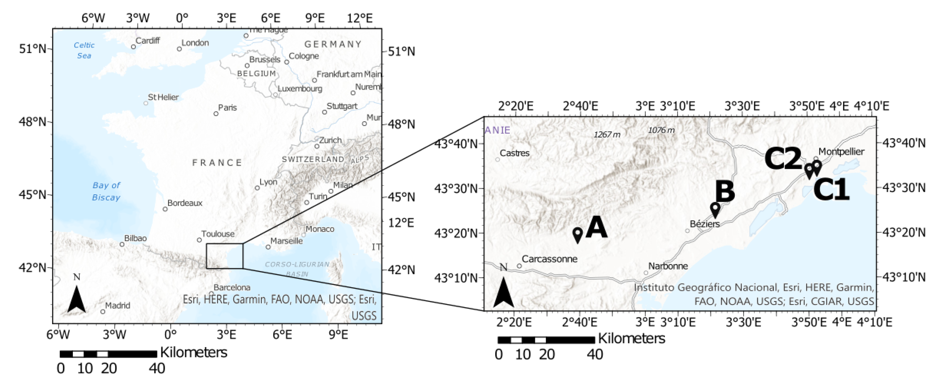
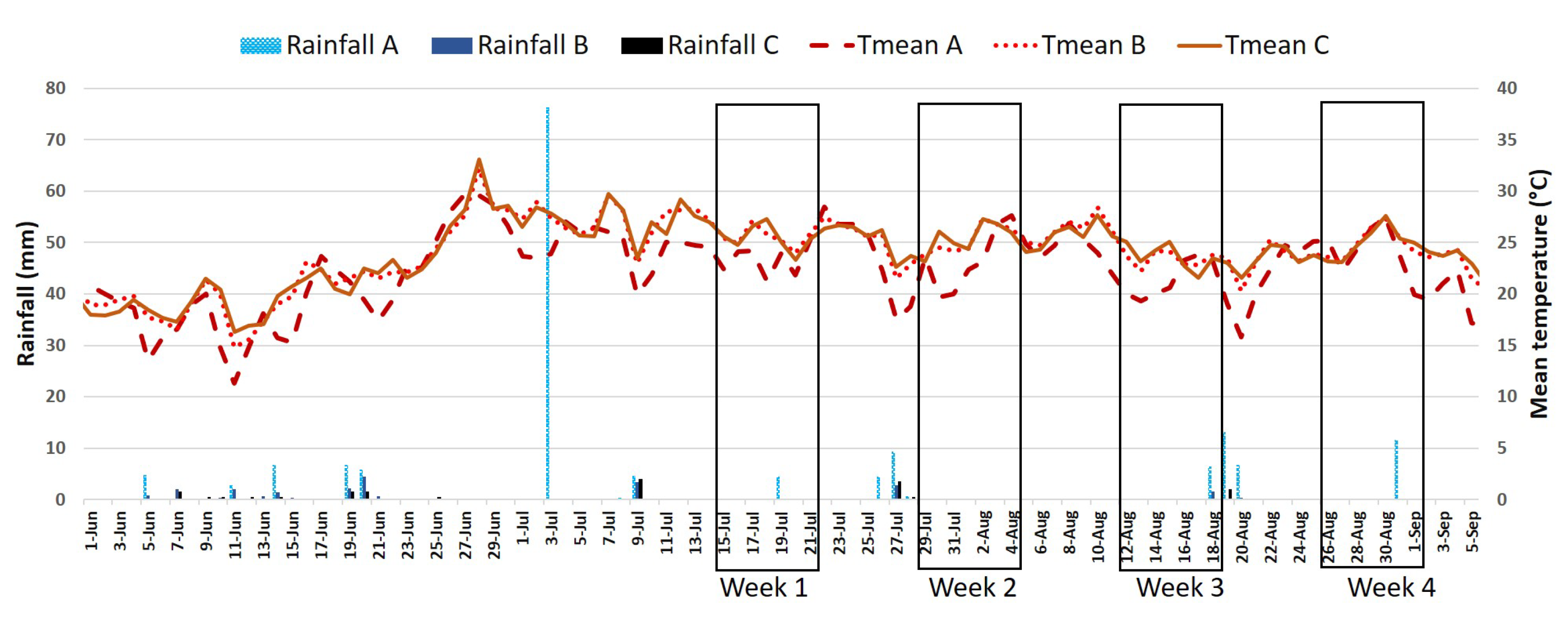
2.1. Study Sites
2.2. Experimental Design
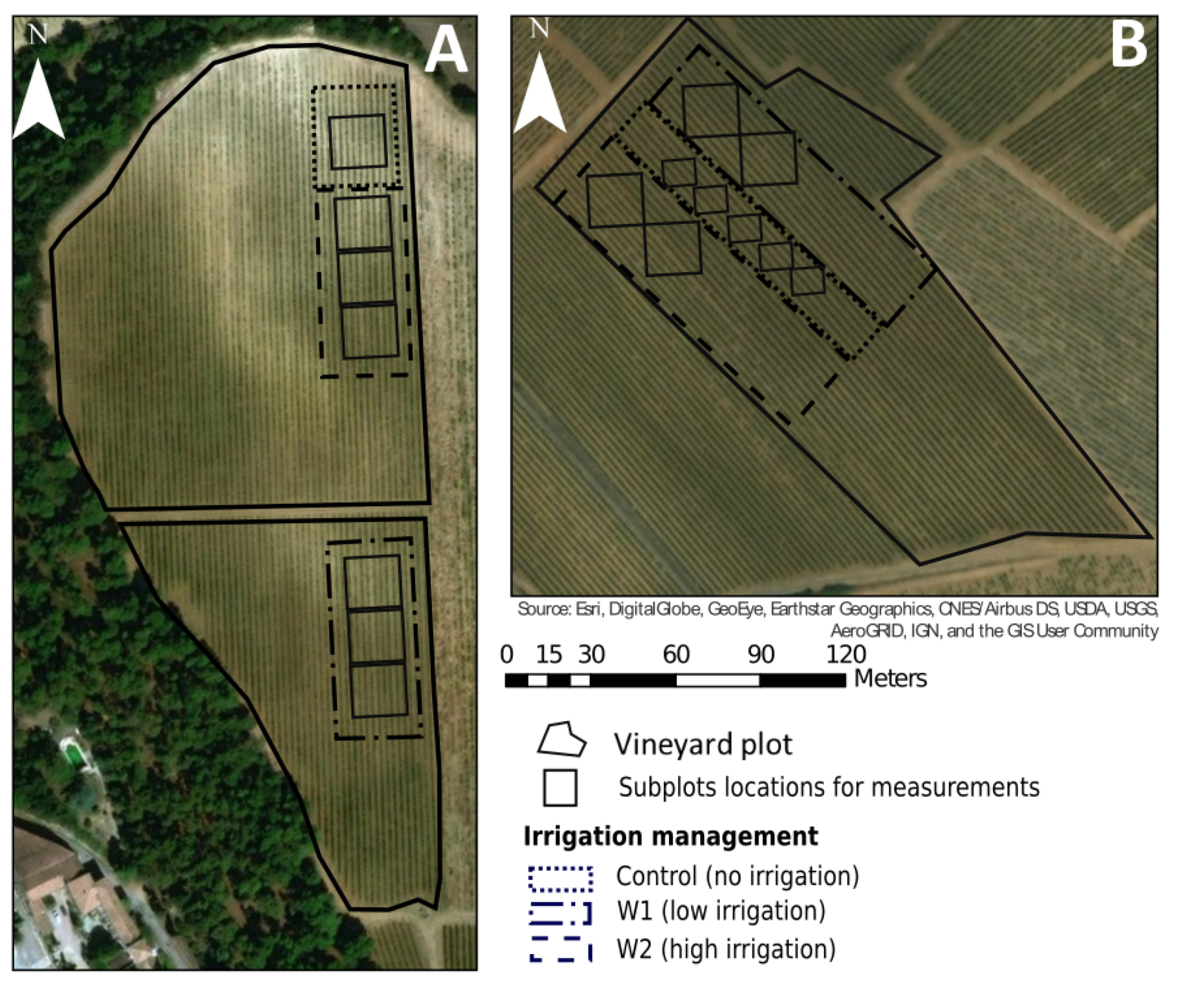
2.2.1. Irrigated Test Plots (A and B)
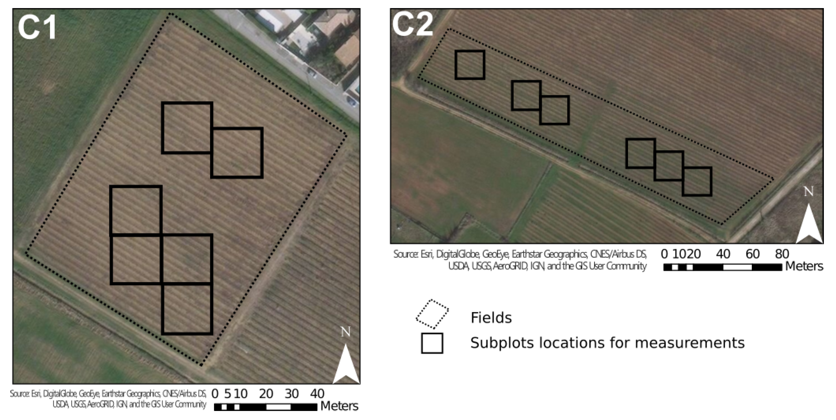
2.2.2. Nonirrigated Plots (C1 and C2)
2.3. Field Measurements
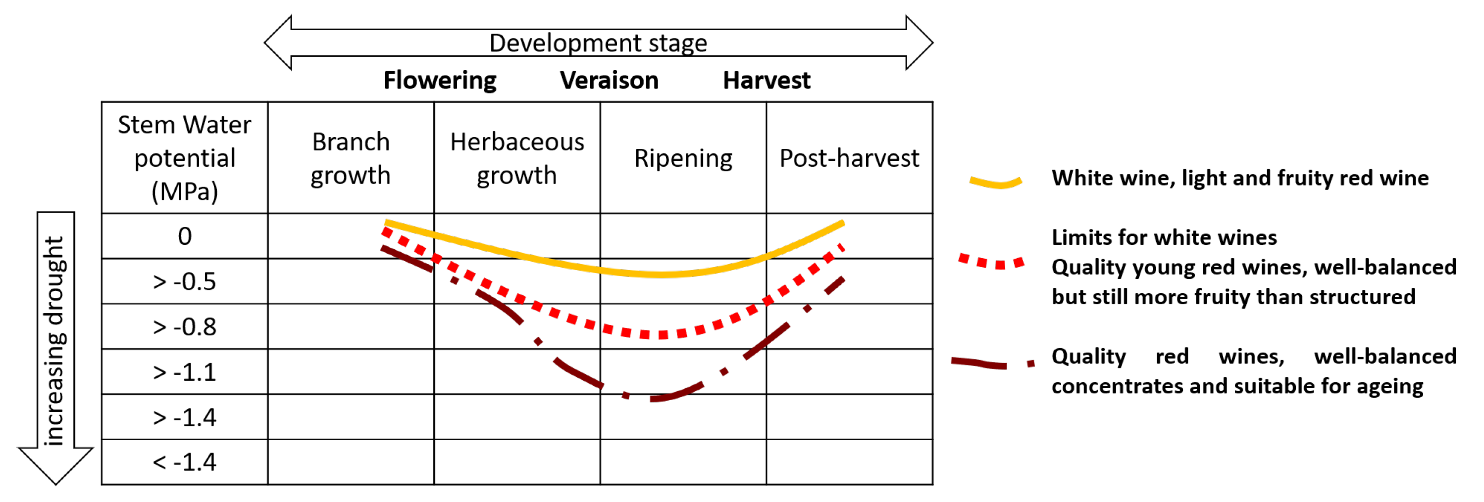
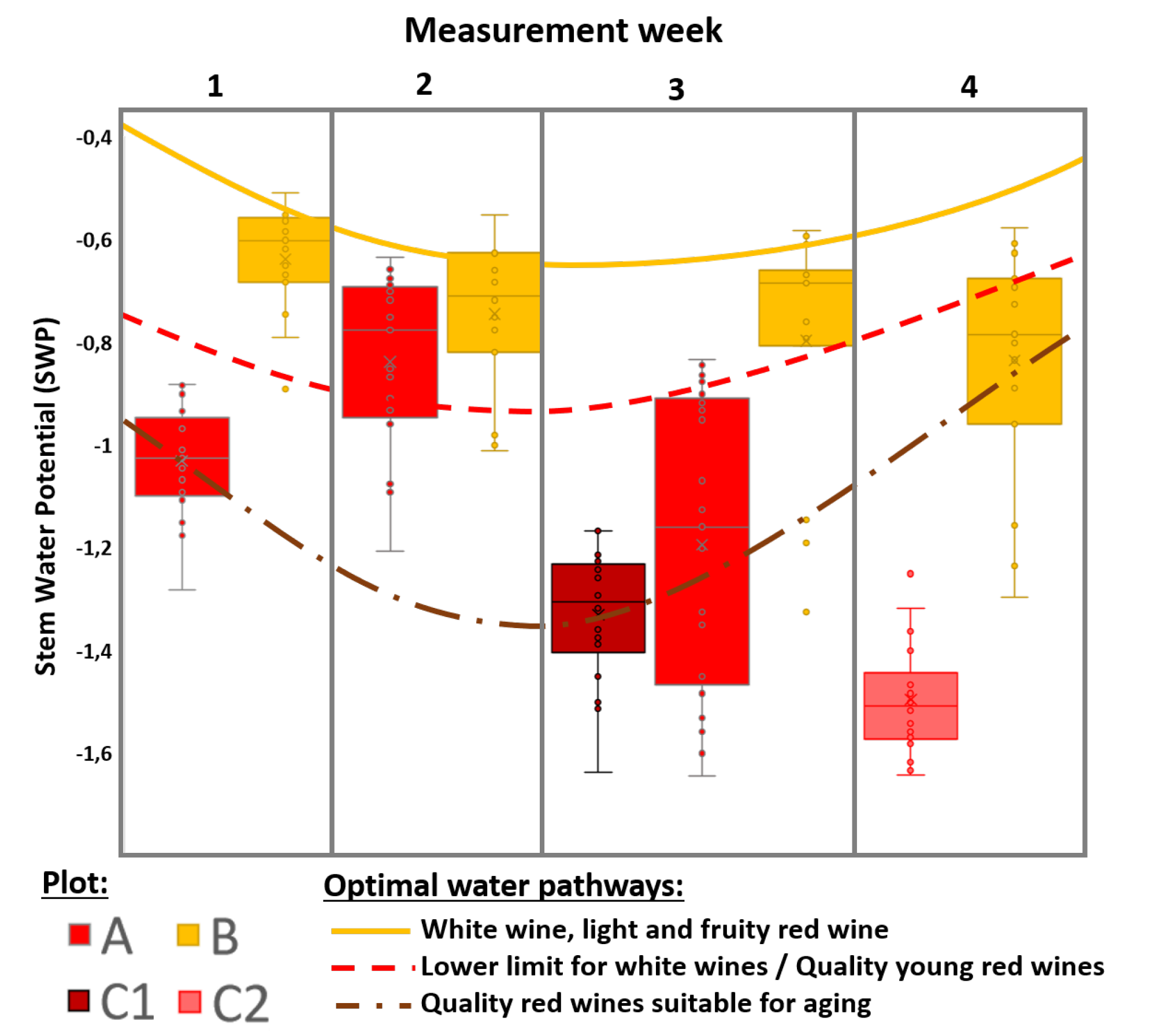
2.3.1. Water Status and SWP Data Set
- SWP data acquisition
- SWP data set description
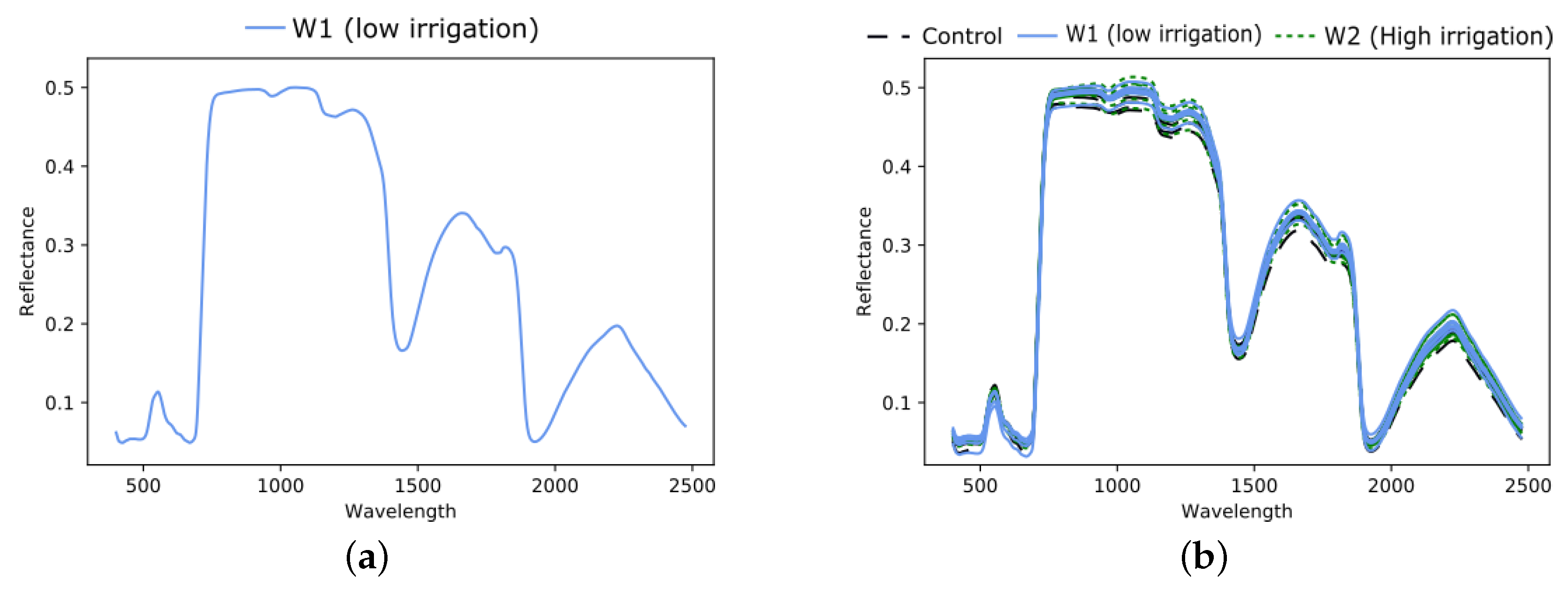
2.3.2. Visible–Near-Infrared (VNIR)/SWIR Reflectance Spectra
- The spectrometer was calibrated using a white reference (Spectralon panel) and a dark current correction was applied. Such calibration is performed every 15 to 30 min to take into account temperature changes over the day.
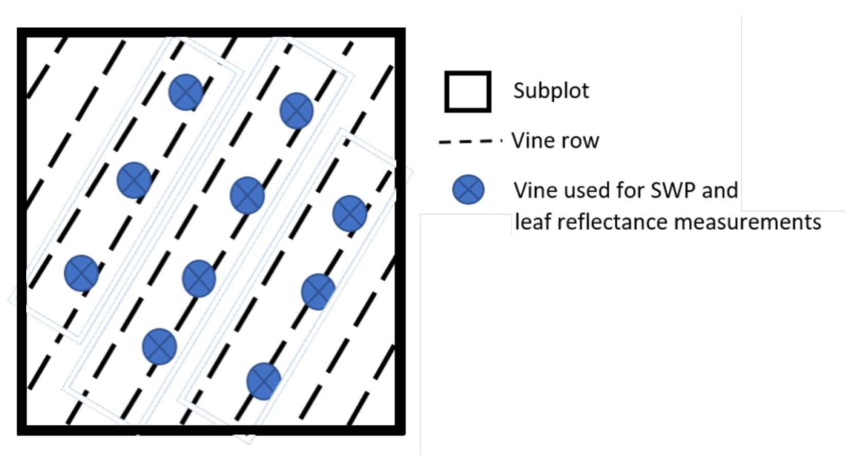
- Three to five raw spectra were acquired on each vine stock, on healthy, young, and mature leaves located preferentially at the top of foliage (i.e., the ones that could be more easily observed from unmanned aerial vehicles (UAVs) or satellites). The measurements were acquired during the whole summer by only two people, alternately and during the day, to minimize operator variability in selection of leaves. Each spectrum is an average of 30 repeated scans. GPS coordinates were also automatically associated to each spectra during the acquisition process.
- Each raw spectrum was ultimately converted to reflectance and exported into an ASCII file using the manufacturer’s ViewSpec Pro software.
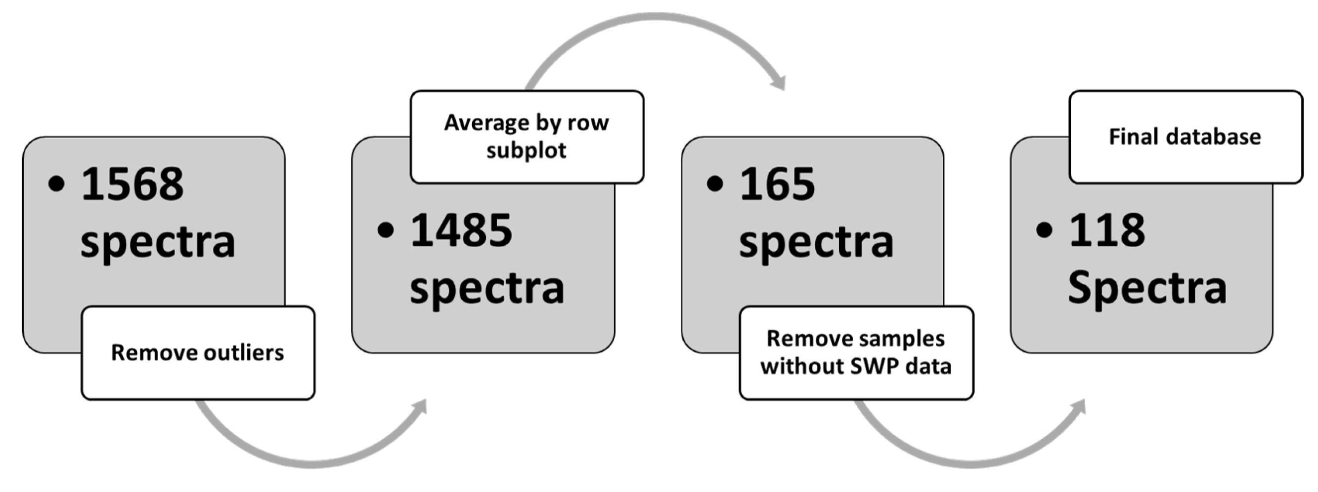
- The last step of preprocessing consisted of checking all spectra to remove outliers according to their reflectance values especially the ones that had a low reflectance level due to measurement error. Spectra were then averaged by row subplot. Samples without SWP measurements for the considered date were also removed from the database (e.g., data for plot A and week 4, as mentioned in Table 3).
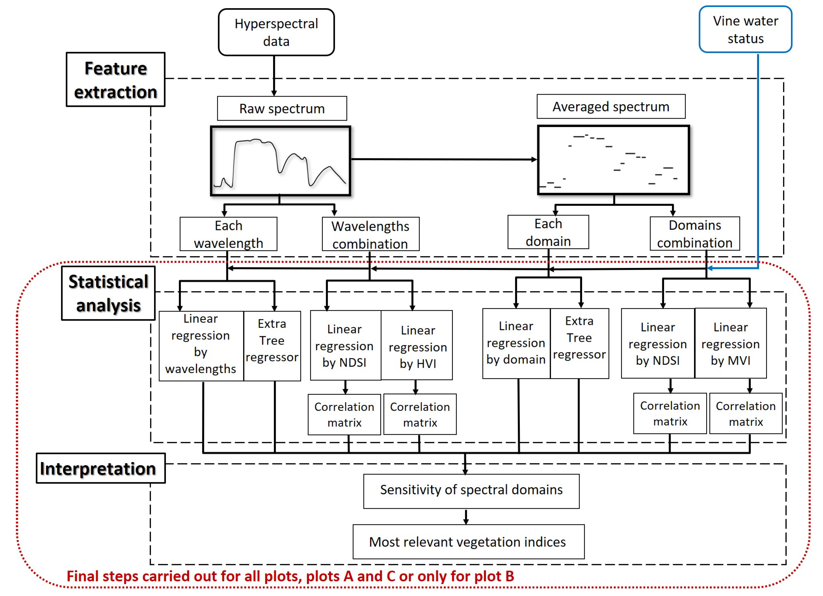
3. Methods
3.1. Feature Extraction
3.1.1. Raw Spectrum
- Using each wavelength separately:The first feature set consists of the leaves’ reflectance values using all the available 1974 wavelengths separately.
- Using wavelength combinations:The second feature set relies on the combination of reflectances at multiple wavelengths. To achieve this, two types of combination were tested: (1) the Normalized Difference Spectral Index (NDSI) and (2) the existing Hyperspectral Vegetation Indices (HVI):
- -
- In the case of NDSI, a feature data set is constructed using two-wavelength combinations ([46,47,48]) in following the formula:where Ri and Rj refer to the reflectance values at λi and λj, respectively. This way, each possible combination of wavelengths over the whole spectrum was systematically tested. This approach allows us to normalize the reflectance and provide a clear overview of the most significant wavelengths. The spectral domains are directly highlighted in the correlation matrix (see Section 3.2.1). Several studies demonstrated that NDSI often performs better than common published indices [49,50].
- -
- The seven most widely used HVIs have been selected for evaluation in this study (Table 5). These indices are known to be linked to the plants’ water status, either directly or using an index related to chlorophyll (itself affected by water content). HVI relies on the combination of two or more wavelengths and each of them is designed to highlight a specific physical property of vegetation.
3.1.2. Average Spectrum by Domains
- This time, NDSIs are computed for each domain (D) according to this formula:where Di and Dj refer to the averaged reflectance values for the domains i and j, respectively. This way, each possible combination of domains is systematically tested.
- Seven MVIs were selected on the basis of both indices found in the literature and our previous analyses using every wavelength. Literature indices not relying on the identified wavelengths range were discarded. These selected MVIs are mostly linked to chlorophyll content. Nevertheless, in order to take into account domains linked directly with water absorption, two HVIs were specifically adapted with relevant SWIR domains. All the selected indices were computed according to the formulas in Table 7.
3.1.3. Available Data Set Summary
3.2. Statistical Analysis
3.2.1. Linear Regression
- With a simple line graph for linear regression by wavelengths;
- With a correlation matrix for NDSI, HVI, and MVI, to compare features’ performance and highlight visually which wavelength ranges or domains are the most significant to extract water status from spectral measurements.
3.2.2. Extra Trees Model
3.3. Results Interpretation
4. Results
4.1. Correlation between SWP and Leaves’ Raw Spectra
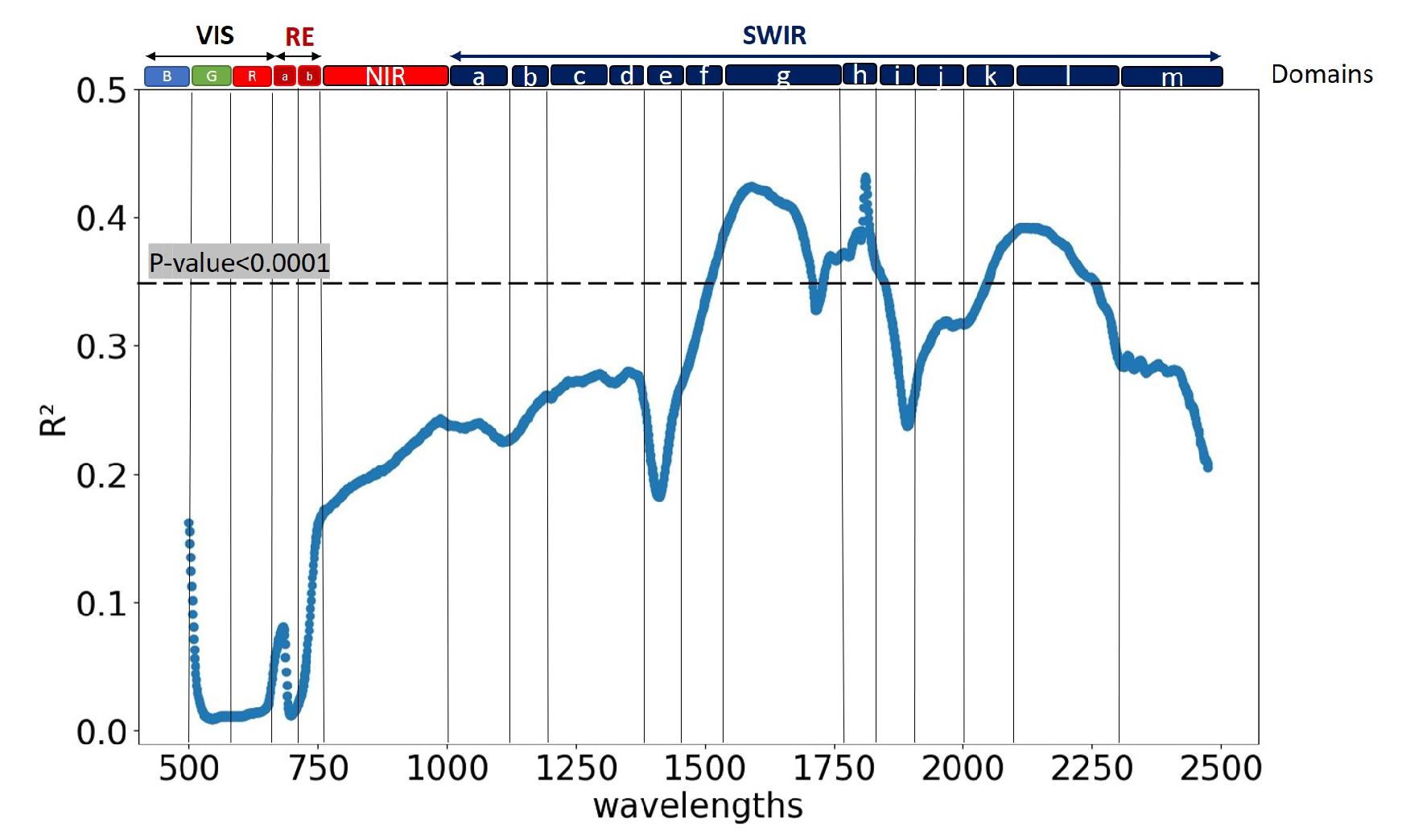
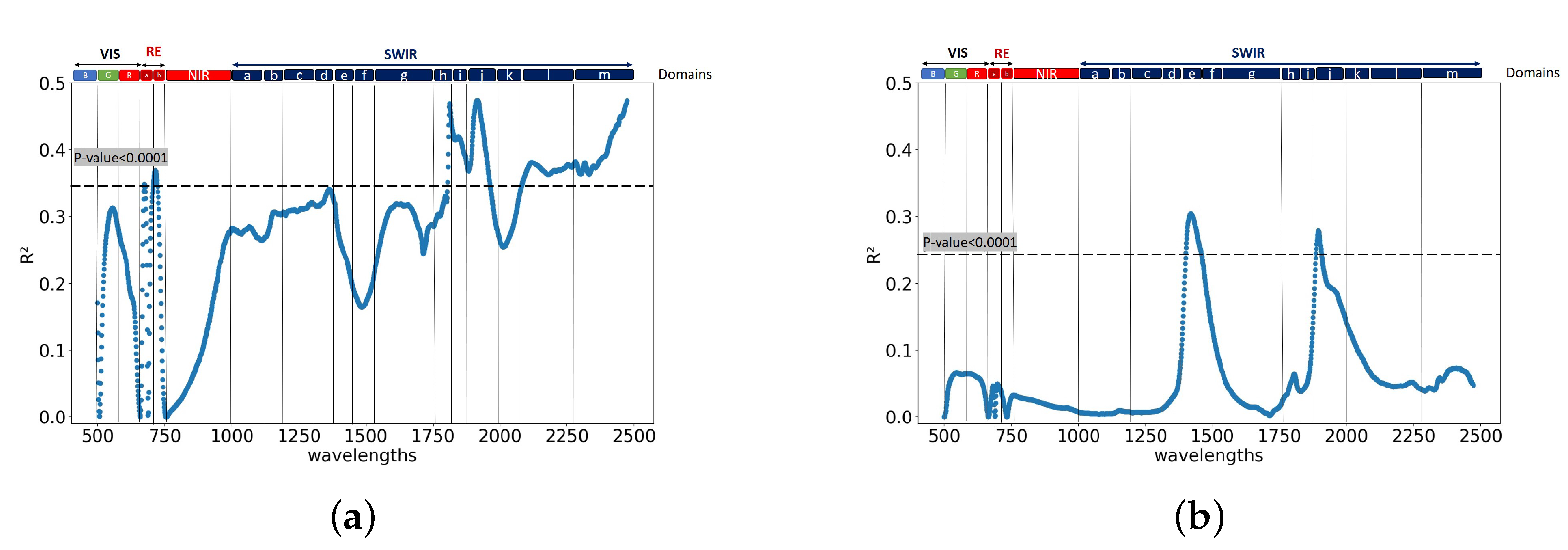
4.1.1. Linear Regression between SWP and Raw Wavelengths
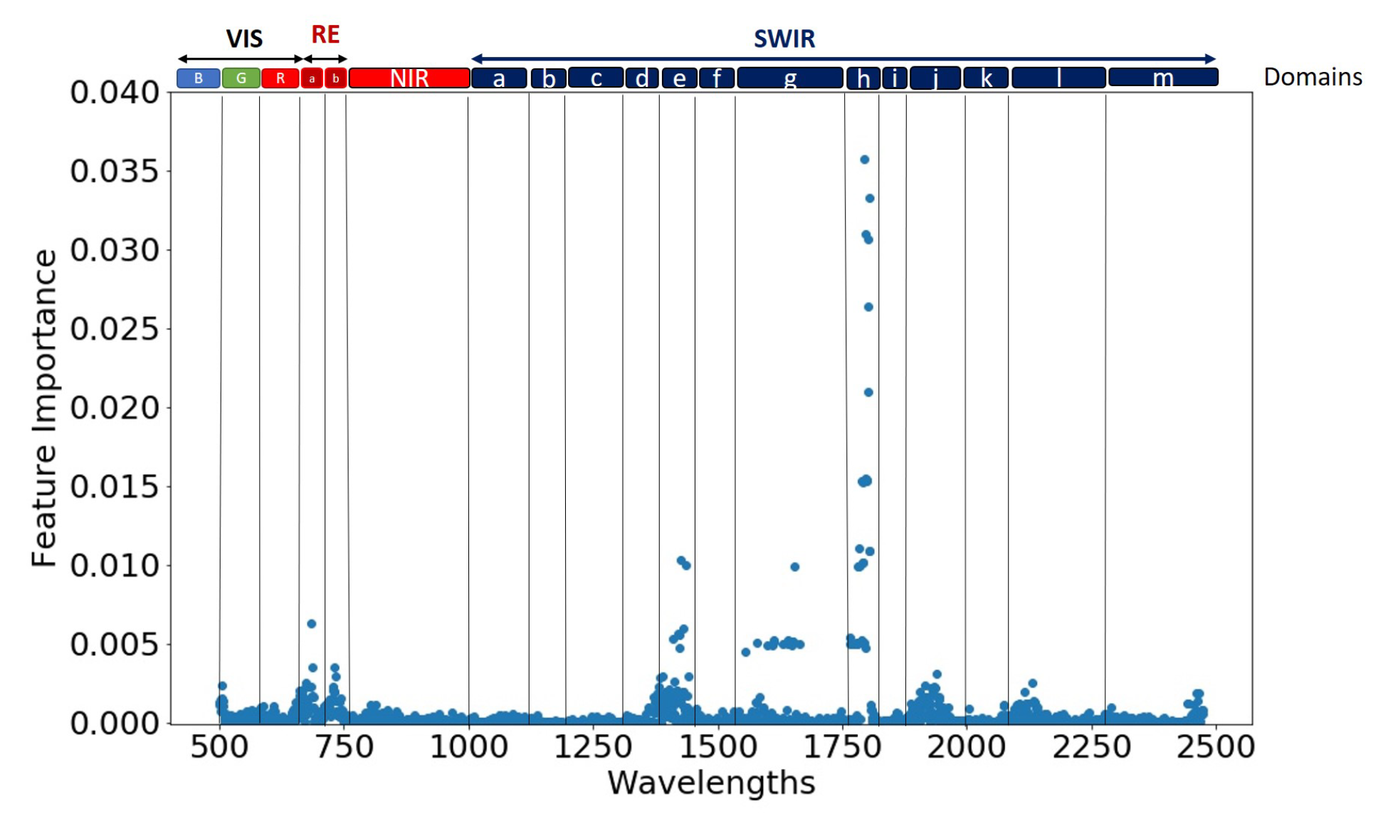
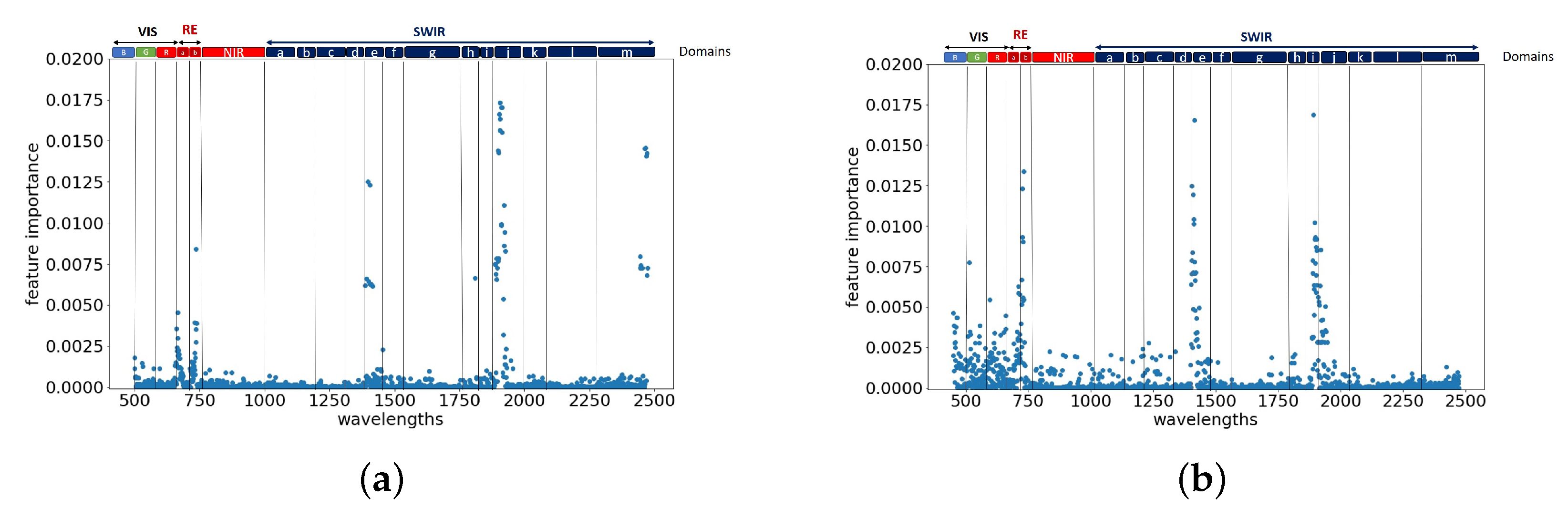
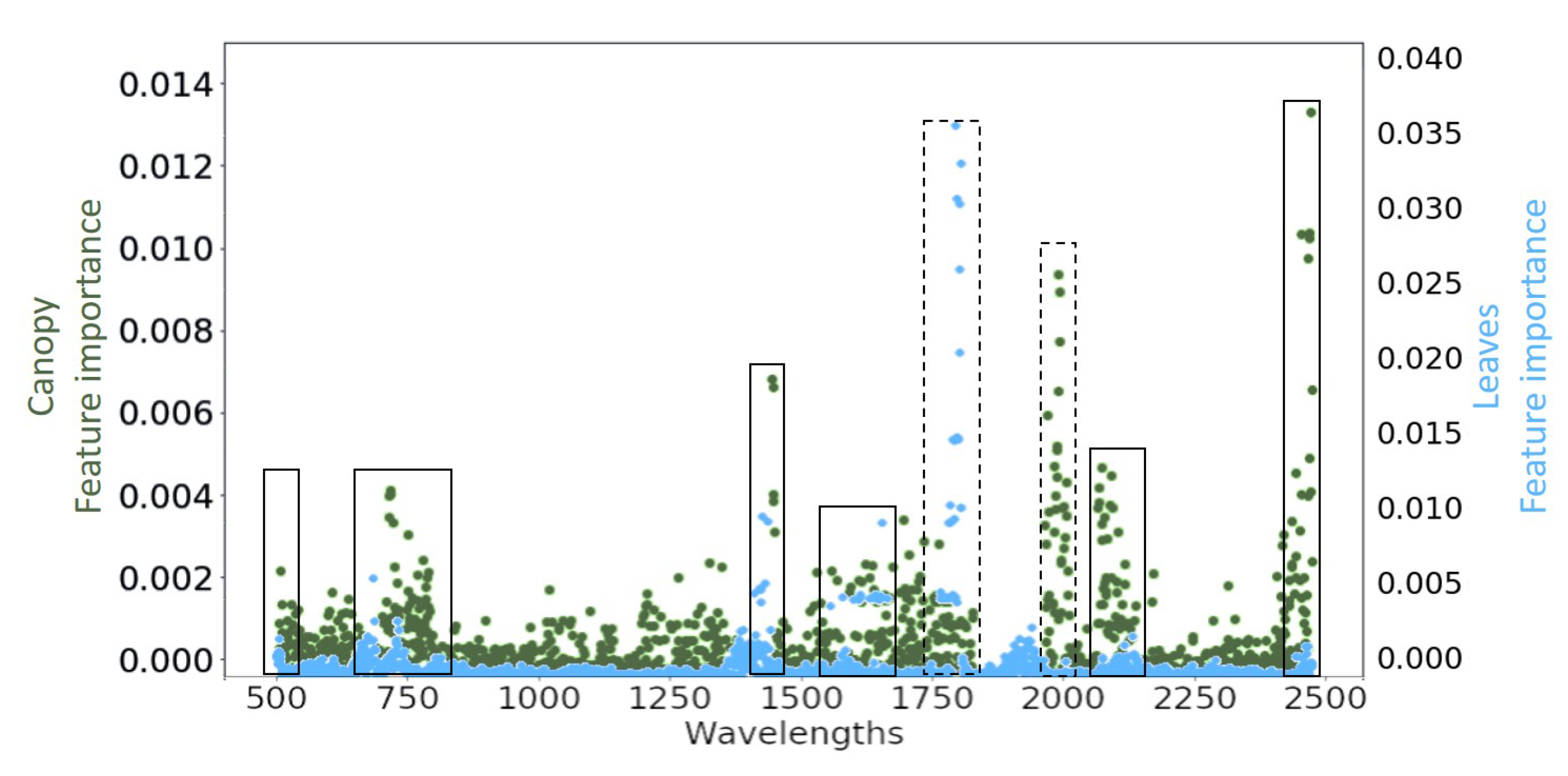
4.1.2. ExtraTree Regression between SWP and Raw Wavelengths
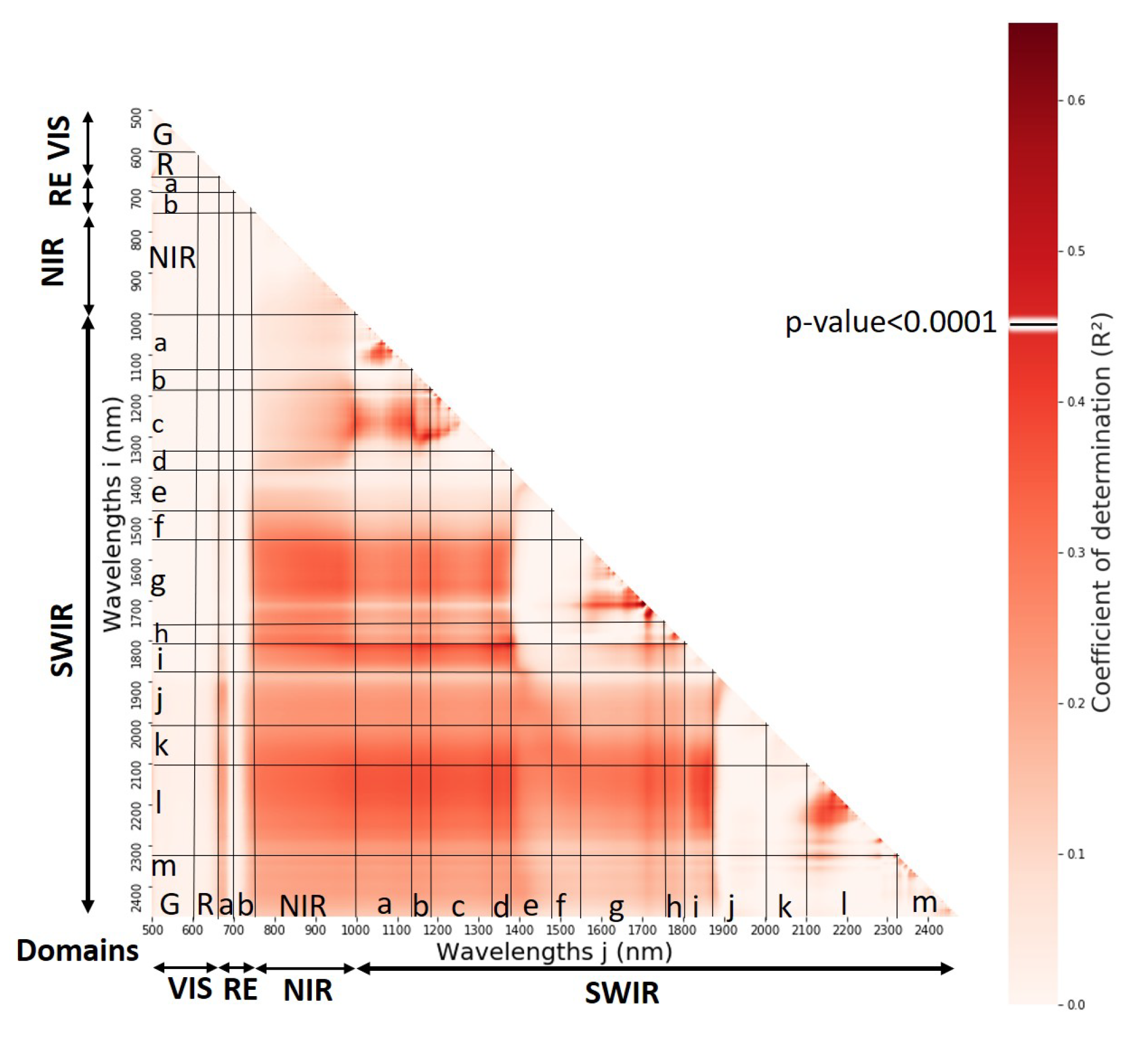
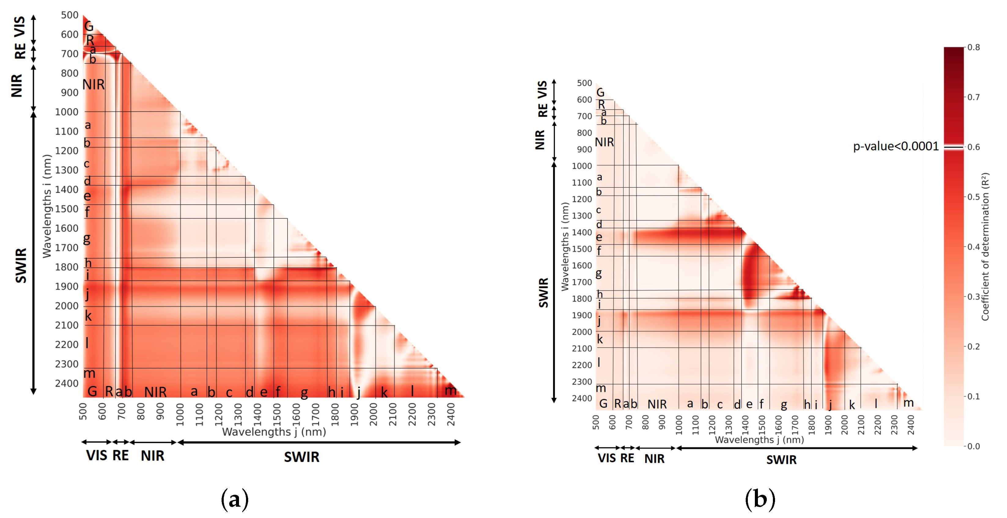
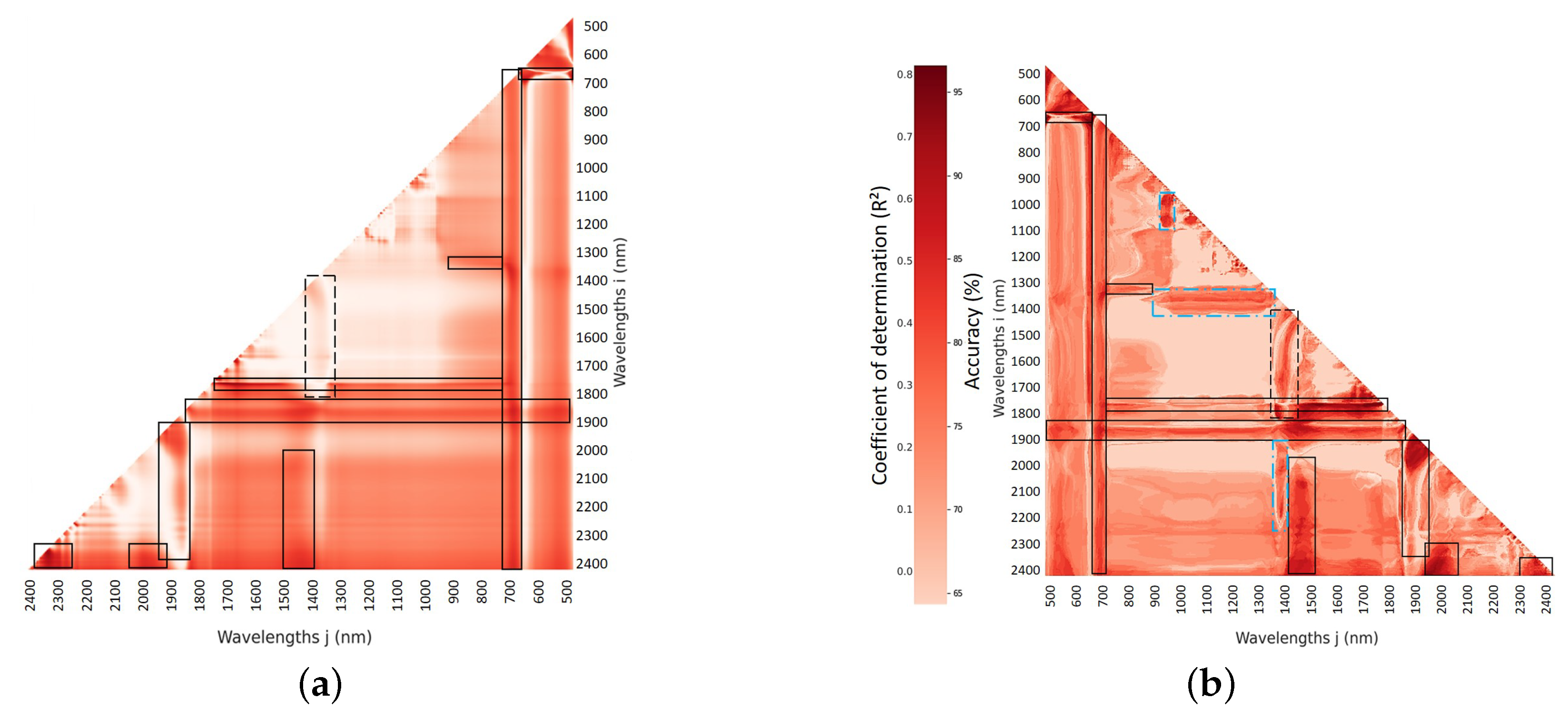
4.1.3. Linear Regression between SWP and NDSI Using Raw Spectra
- From the 800 to 1400 nm range with wavelengths (i) around 1800 nm, (ii) from the 2100 to 2300 nm range, and (iii) from the 1550 to 1700 nm range;
- From the 1800 to 1900 nm range with wavelengths from the 2150 to 2300 nm range;
- From the 670 to 700 nm range with wavelengths from the 1900 to 2400 nm range.
- From the 700 to 750 nm range with wavelengths from the 700 to 2400 nm range;
- From the 500 to 600 nm range with wavelengths from the 600 to 700 nm range;
- From the 500 to 1900 nm range with wavelengths around 1900 nm;
- From the 1600 to 1800 nm range with wavelengths around 1800 nm.
- From the 800 to 1400 nm range with wavelengths (i) around 1900 nm and (ii) from the 1400 to 1500 nm range;
- From the 1400 to 1500 nm range with wavelengths from the 1500 to 1800 nm range;
- From the 1900 to 2000 nm range with wavelengths from the 2000 to 2400 nm range;
- From the 1650 to 1800 nm range with wavelengths from the 1800 to 1850 nm range.
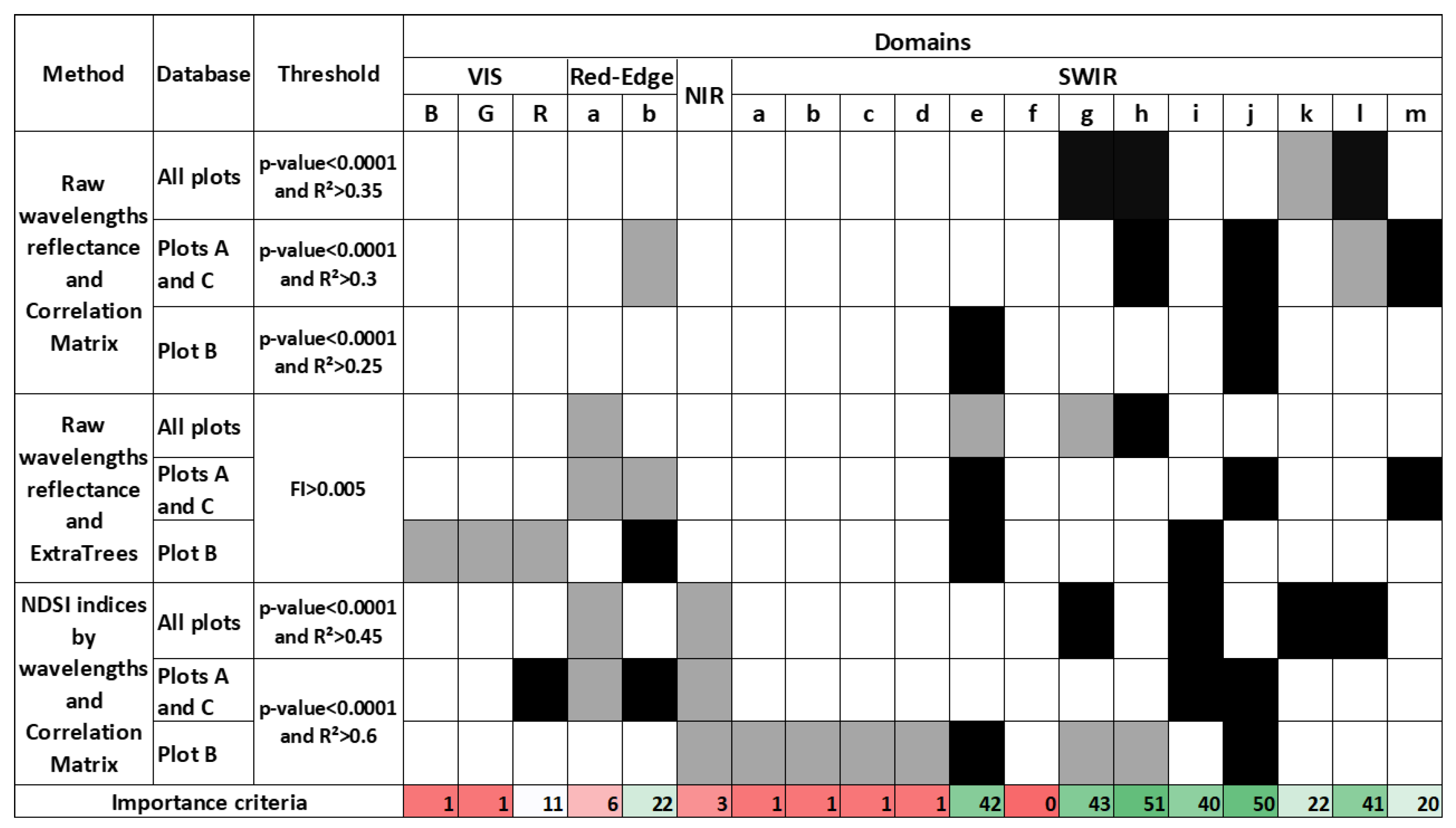
4.1.4. Summary of the Results for All Correlations Tested on Raw Spectra
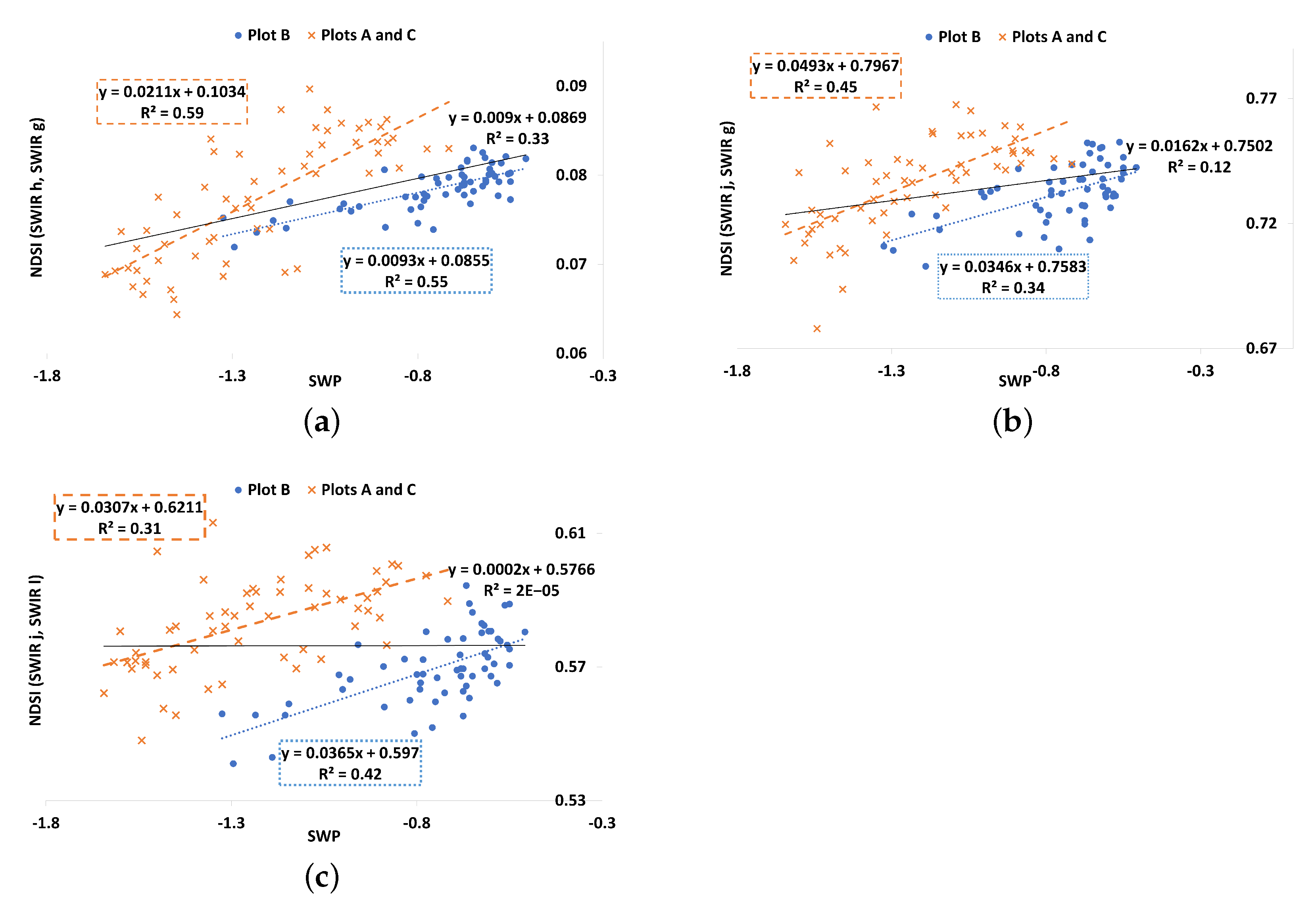
4.1.5. Linear Regression between SWP and Hyperspectral Vegetation Indices
- Normalized Difference Water Index (NDWI) with wavelength reflectance in “SWIR c” and “NIR”;
- Moisture Stress Index (MSI) with wavelength reflectance in “SWIR g” and “NIR”.
- CI with wavelength reflectance in “Red-Edge a” and “Red-Edge b”;
- MSI with wavelength reflectance in “SWIR g” and “NIR”;
- NDWI with wavelength reflectance in “SWIR c” and “NIR”;
- WBI with wavelength reflectance in “NIR”.
4.2. Correlation between SWP and Leaves’ Spectra Averaged by Domains
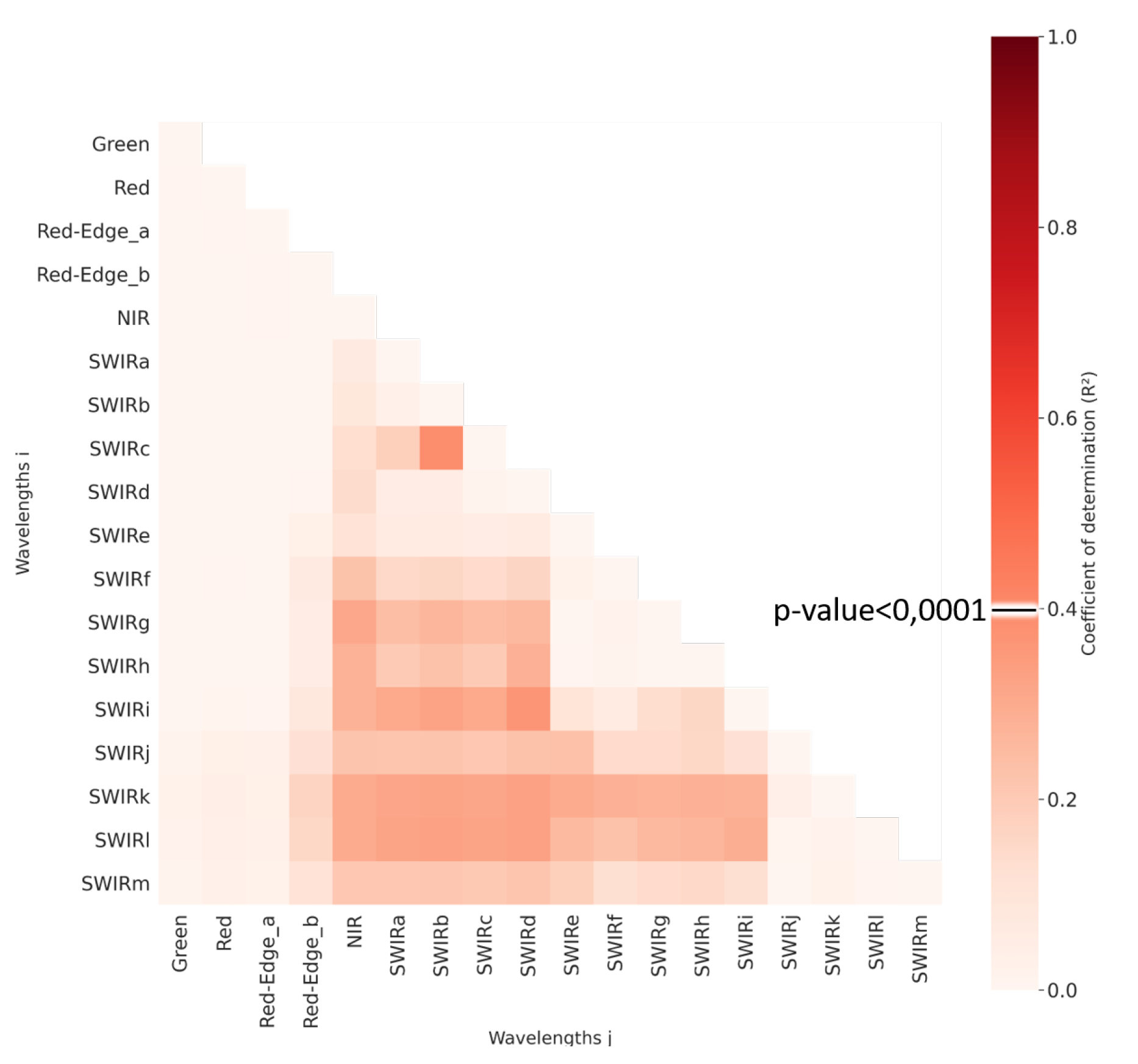
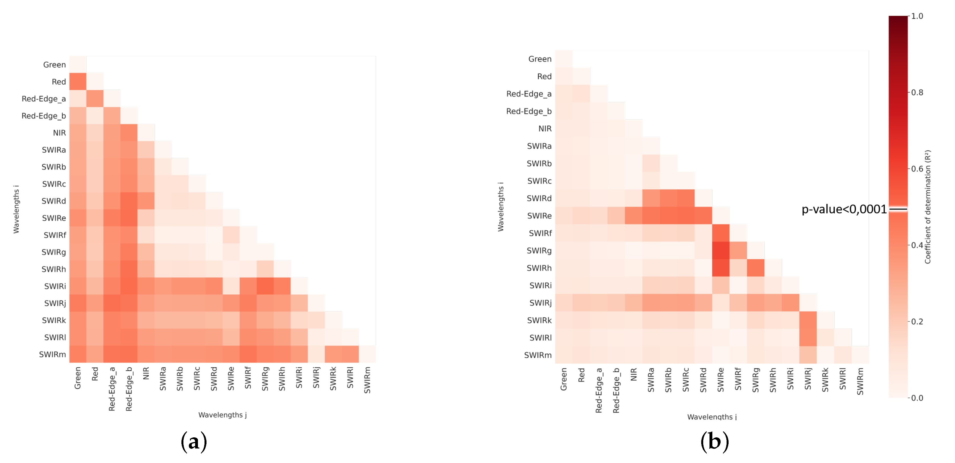
4.2.1. Linear Regression between SWP and NDSI Using Domains
- “SWIR c” with “SWIR b”;
- “SWIR i” with “SWIR d”;
- “SWIR k” and “SWIR l” with “NIR” to “SWIR d”;
- “SWIR g” with “NIR”.
- “Red-Edge a” with “SWIR j” and “SWIR m”;
- “Red-Edge b” with “SWIR d”, “SWIR e”, “SWIR h”, and “SWIR i”;
- “SWIR g” with “SWIR i”.
- “SWIR e” with “NIR” and “SWIR a” to “SWIR h”;
- “SWIR d” with “SWIR a”, “SWIR b”, and “SWIR c”;
- “SWIR j” with (i) “SWIR a” to “SWIR d” and (ii) “SWIR g” to “SWIR l”.
4.2.2. Linear Regression between SWP and Multispectral Vegetation Indices
5. Discussion
5.1. Summary of the Results
5.2. Spectral Domain and VI Sensitivity
5.3. Correlation Differences between Wavelengths and Domain Reflectance
5.4. Correlation Differences between Plots
5.5. Choice of Analysis Method
5.6. From Hyperspectral to Multispectral Data
6. Conclusions
Author Contributions
Funding
Data Availability Statement
Acknowledgments
Conflicts of Interest
Abbreviations
| EnMAP | Environmental Mapping and Analysis Program |
| EO | Earth Observation |
| FI | Feature importance |
| GNSS | Global Navigation Satellite System |
| HVI | Hyperspectral vegetation indices |
| HySIS | Hyperspectral Imaging Satellite |
| IC | Importance Criteria |
| Kc | Crop Coefficient |
| mm | millimeter |
| MPa | Mega Pascal |
| MVI | Multispectral vegetation indices |
| N | Nitrogen |
| ND | NoData |
| NDSI | Normalized Difference Spectral Index |
| nm | nanometer |
| µm | micrometer |
| NIR | Near Infrared |
| PCA | Principal Component Analysis |
| PLS-r | Partial Least Square regression |
| PRISMA | PRecursore IperSpettrale della Missione Applicativa |
| RE | Red-Edge |
| RMSE | Root Mean Square Error |
| S2 | Sentinel-2 |
| SVM | Support Vector Machine |
| SWP | Stem Water Potential |
| SWIR | Short-Wave Infrared |
| UAV | unmanned aerial vehicle |
| VI | Vegetation Index |
| VIS | Visible |
| VNIR | Visible–Near-Infrared |
References
- Van Leeuwen, C.; Trégoat, O.; Choné, X.; Jaeck, M.E.; Gaudillere, J.P. Assessment of vine water uptake conditions and its influence on fruit ripening. Bulletin l’OIV 2003, 76, 367–378. [Google Scholar]
- Potopová, V.; Trnka, M.; Hamouz, P.; Soukup, J.; Castraveț, T. Statistical modelling of drought-related yield losses using soil moisture-vegetation remote sensing and multiscalar indices in the south-eastern Europe. Agric. Water Manag. 2020, 236, 106168. [Google Scholar] [CrossRef]
- Ojeda, H.; Saurin, N. L’irrigation de précision de la vigne: Méthodes, outils et stratégies pour maximiser la qualité et les rendements de la vendange en économisant de l’eau. Innov. Agron. 2014, 38, 97–108. [Google Scholar]
- Bernardo, S.; Dinis, L.T.; Machado, N.; Moutinho-Pereira, J. Grapevine abiotic stress assessment and search for sustainable adaptation strategies in Mediterranean-like climates. A review. Agron. Sustain. Dev. 2018, 38. [Google Scholar] [CrossRef] [Green Version]
- Monteiro, A.; Lopes, C.M. Influence of cover crop on water use and performance of vineyard in Mediterranean Portugal. Agric. Ecosyst. Environ. 2007, 121, 336–342. [Google Scholar] [CrossRef]
- Catania, P.; Badalucco, L.; Laudicina, V.A.; Vallone, M. Effects of tilling methods on soil penetration resistance, organic carbon and water stable aggregates in a vineyard of semiarid Mediterranean environment. Environ. Earth Sci. 2018, 77, 348. [Google Scholar] [CrossRef]
- Costa, J.M.; Vaz, M.; Escalona, J.; Egipto, R.; Lopes, C.; Medrano, H.; Chaves, M.M. Modern viticulture in southern Europe: Vulnerabilities and strategies for adaptation to water scarcity. Agric. Water Manag. 2015, 164, 5–18. [Google Scholar] [CrossRef]
- Quenol, H.; De Cortazar Atauri, I.G.; Bois, B.; Sturman, A.; Bonnardot, V.; Le Roux, R.; Ollat, N. Which climatic modeling to assess climate change impacts on vineyards? Oeno One 2017, 51, 91–97. [Google Scholar] [CrossRef] [Green Version]
- Brillante, L.; Martinez-Luscher, J.; Yu, R.; Plank, C.M.; Sanchez, L.; Bates, T.L.; Brenneman, C.; Oberholster, A.; Kurtural, S.K. Assessing Spatial Variability of Grape Skin Flavonoids at the Vineyard Scale Based on Plant Water Status Mapping. J. Agric. Food Chem. 2017, 65, 5255–5265. [Google Scholar] [CrossRef]
- Ramos, M.C.; Perez-Alvarez, E.P.; Peregrina, F.; Martinez de Toda, F. Relationships between grape composition of Tempranillo variety and available soil water and water stress under different weather conditions. Sci. Hortic. 2020, 262, 109063. [Google Scholar] [CrossRef]
- Tomás, M.; Medrano, H.; Escalona, J.M.; Martorell, S.; Pou, A.; Ribas-Carbó, M.; Flexas, J. Variability of water use efficiency in grapevines. Environ. Exp. Bot. 2014, 103, 148–157. [Google Scholar] [CrossRef]
- Williams, L.E. Physiological tools to assess vine water status for use in vineyard irrigation management: Review and update. Acta Hortic. 2017, 1157, 151–166. [Google Scholar] [CrossRef]
- Saurin, N.; Tisseyre, B.; Lebon, E. Comment mesurer la contrainte hydrique de la vigne, de la plante au vignoble. Innov. Agron. 2014, 38, 143–158. [Google Scholar]
- Choné, X.; Van Leeuwen, C.; Dubourdieu, D.; Gaudillère, J.P. Stem water potential is a sensitive indicator of grapevine water status. Ann. Bot. 2001, 87, 477–483. [Google Scholar] [CrossRef] [Green Version]
- Acevedo-Opazo, C.; Tisseyre, B.; Ojeda, H.; Guillaume, S. Spatial extrapolation of the vine (Vitis vinifera L.) water status: A first step towards a spatial prediction model. Irrig. Sci. 2009, 28, 143–155. [Google Scholar] [CrossRef]
- Romero-Trigueros, C.; Bayona Gambín, J.M.; Nortes Tortosa, P.A.; Alarcón Cabañero, J.J.; Nicolás Nicolás, E. Determination of Crop Water Stress Index by Infrared Thermometry in Grapefruit Trees Irrigated with Saline Reclaimed Water Combined with Deficit Irrigation. Remote Sens. 2019, 11, 757. [Google Scholar] [CrossRef] [Green Version]
- Transon, J.; D’Andrimont, R.; Maugnard, A.; Defourny, P. Survey of hyperspectral Earth Observation applications from space in the Sentinel-2 context. Remote Sens. 2018, 10, 157. [Google Scholar] [CrossRef] [Green Version]
- Weiss, M.; Jacob, F.; Duveiller, G. Remote sensing for agricultural applications: A meta-review. Remote Sens. Environ. 2020, 236, 111402. [Google Scholar] [CrossRef]
- Ferrant, S.; Selles, A.; Le Page, M.; Herrault, P.A.; Pelletier, C.; Al-Bitar, A.; Mermoz, S.; Gascoin, S.; Bouvet, A.; Saqalli, M.; et al. Detection of irrigated crops from Sentinel-1 and Sentinel-2 data to estimate seasonal groundwater use in South India. Remote Sens. 2017, 9, 1119. [Google Scholar] [CrossRef] [Green Version]
- Rozenstein, O.; Haymann, N.; Kaplan, G.; Tanny, J. Estimating cotton water consumption using a time series of Sentinel-2 imagery. Agric. Water Manag. 2018, 207, 44–52. [Google Scholar] [CrossRef]
- Devaux, N.; Crestey, T.; Leroux, C.; Tisseyre, B. Potential of Sentinel-2 satellite images to monitor vine fields grown at a territorial scale. Oeno One 2019, 53, 51–58. [Google Scholar] [CrossRef]
- Di Gennaro, S.F.; Dainelli, R.; Palliotti, A.; Toscano, P.; Matese, A. Sentinel-2 validation for spatial variability assessment in overhead trellis system viticulture versus UAV and agronomic data. Remote Sens. 2019, 11, 2573. [Google Scholar] [CrossRef] [Green Version]
- Cogato, A.; Pagay, V.; Marinello, F.; Meggio, F.; Grace, P.; De Antoni Migliorati, M. Assessing the Feasibility of Using Sentinel-2 Imagery to Quantify the Impact of Heatwaves on Irrigated Vineyards. Remote Sens. 2019, 11, 2869. [Google Scholar] [CrossRef] [Green Version]
- Cohen, Y.; Gogumalla, P.; Bahat, I.; Netzer, Y.; Ben-Gal, A.; Lenski, I.; Michael, Y.; Helman, D. Can time series of multispectral satellite images be used to estimate stem water potential in vineyards. In Precision Agriculture’19; Wageningen Academic Publishers: Wageningen, The Netherlands, 2019; pp. 445–451. [Google Scholar] [CrossRef]
- Gao, Y.; Qiu, J.; Miao, Y.; Qiu, R.; Li, H.; Zhang, M. Prediction of Leaf Water Content in Maize Seedlings Based on Hyperspectral Information. IFAC-Pap. Online 2019, 52, 263–269. [Google Scholar] [CrossRef]
- Rapaport, T.; Hochberg, U.; Shoshany, M.; Karnieli, A.; Rachmilevitch, S. Combining leaf physiology, hyperspectral imaging and partial least squares-regression (PLS-R) for grapevine water status assessment. ISPRS J. Photogramm. Remote Sens. 2015, 109, 88–97. [Google Scholar] [CrossRef]
- Loggenberg, K.; Strever, A.; Greyling, B.; Poona, N. Modelling water stress in a Shiraz vineyard using hyperspectral imaging and machine learning. Remote Sens. 2018, 10, 202. [Google Scholar] [CrossRef] [Green Version]
- Zovko, M.; Zibrat, U.; Knapic, M.; Bubalo Kovacic, M.; Romic, D. Hyperspectral remote sensing of grapevine drought stress. Precis. Agric. 2019, 20, 335–347. [Google Scholar] [CrossRef]
- Zhang, F.; Zhou, G. Estimation of vegetation water content using hyperspectral vegetation indices: A comparison of crop water indicators in response to water stress treatments for summer maize. BMC Ecol. 2019, 19, 18. [Google Scholar] [CrossRef] [Green Version]
- Imanishi, J.; Morimoto, Y.; Imanishi, A.; Sugimoto, K.; Isoda, K. The independent detection of drought stress and leaf density using hyperspectral resolution data. Landsc. Ecol. Eng. 2007, 3, 55–65. [Google Scholar] [CrossRef]
- Ranjan, R.; Sahoo, R.N.; Chopra, U.K.; Pramanik, M.; Singh, A.K.; Pradhan, S. Assessment of Water Status in Wheat (Triticum aestivum L.) Using Ground Based Hyperspectral Reflectance. Proc. Natl. Acad. Sci. India Sect. B Biol. Sci. 2017, 87, 377–388. [Google Scholar] [CrossRef]
- Surase, R.R.; Kale, K.V.; Varpe, A.B.; Vibhute, A.D.; Gite, H.R.; Solankar, M.M.; Gaikwad, S.; Nalawade, D.B. Estimation of Water Contents from Vegetation Using Hyperspectral Indices. In Microelectronics, Electromagnetics and Telecommunications, Lecture Notes in Electrical Engineering 521; Lecture Notes in Electrical Engineering, Anguera, J., Satapathy, S.C., Bhateja, V., Sunitha, K., Eds.; Springer: Singapore, 2019; Volume 471, pp. 247–255. [Google Scholar] [CrossRef]
- Seelig, H.D.; Hoehn, A.; Stodieck, L.S.; Klaus, D.M.; Adams, W.W., III; Emery, W.J. Plant water parameters and the remote sensing R 1300/R 1450 leaf water index: Controlled condition dynamics during the development of water deficit stress. Irrig. Sci. 2009, 27, 357–365. [Google Scholar] [CrossRef]
- Rodríguez-Pérez, J.R.; Riaño, D.; Carlisle, E.; Ustin, S.; Smart, D.R. Evaluation of Hyperspectral Reflectance Indexes to Detect Grapevine Water Status in Vineyards. Am. J. Enol. Vitic. 2007, 58, 302–317. [Google Scholar]
- Pôças, I.; Rodrigues, A.; Gonçalves, S.; Costa, P.M.; Gonçalves, I.; Pereira, L.S.; Cunha, M. Predicting grapevine water status based on hyperspectral reflectance vegetation indices. Remote Sens. 2015, 7, 16460–16479. [Google Scholar] [CrossRef] [Green Version]
- Seelig, H.D.; Hoehn, A.; Stodieck, L.S.; Klaus, D.M.; Adams, W.W.; Emery, W.J. The assessment of leaf water content using leaf reflectance ratios in the visible, near-, and short-wave-infrared. Int. J. Remote Sens. 2008, 29, 3701–3713. [Google Scholar] [CrossRef]
- Simonneau, T.; Ollat, N.; Pellegrino, A.; Lebon, E. Contrôle de l’état hydrique dans la plante et réponses physiologiques de la vigne à la contrainte hydrique. Innov. Agron. 2014, 38, 13–82. Available online: http://xxx.lanl.gov/abs/https://www6.inrae.fr/ciag/content/download/%205376/41590/file/Vol38-2-Simonneau.pdf (accessed on 2 February 2021).
- Charrier, G.; Delzon, S.; Domec, J.C.; Zhang, L.; Delmas, C.E.L.; Merlin, I.; Corso, D.; King, A.; Ojeda, H.; Ollat, N.; et al. Drought will not leave your glass empty: Low risk of hydraulic failure revealed by long-term drought observations in world’s top wine regions. Sci. Adv. 2018, 4, 9. [Google Scholar] [CrossRef] [Green Version]
- Sade, N.; Gebremedhin, A.; Moshelion, M. Risk-taking plants. Plant Signal. Behav. 2012, 7, 767–770. [Google Scholar] [CrossRef] [Green Version]
- Munitz, S.; Schwartz, A.; Netzer, Y. Water consumption, crop coe ffi cient and leaf area relations of a Vitis vinifera cv. ‘Cabernet Sauvignon’ vineyard. Agric. Water Manag. 2019, 219, 86–94. [Google Scholar] [CrossRef]
- Hodáňová, D. Leaf Optical Properties. In Photosynthesis during Leaf Development. Tasks for Vegetation Science; Zdenek, Š., Ed.; Springer: Dordrecht, The Netherlands, 1985; Volume 11, pp. 107–127. [Google Scholar] [CrossRef]
- Vane, G.; Goetz, A.F. Terrestrial imaging spectroscopy. Remote Sens. Environ. 1988, 24, 1–29. [Google Scholar] [CrossRef]
- Camps-Valls, G.; Tuia, D.; Gómez-Chova, L.; Jiménez, S.; Malo, J. Remote Sensing Image Processing. Synth. Lect. Image Video Multimed. Process. 2011, 5, 1–192. [Google Scholar] [CrossRef]
- Verrelst, J.; Camps-Valls, G.; Muñoz-Marí, J.; Rivera, J.P.; Veroustraete, F.; Clevers, J.G.; Moreno, J. Optical remote sensing and the retrieval of terrestrial vegetation bio-geophysical properties—A review. ISPRS J. Photogramm. Remote Sens. 2015, 108, 273–290. [Google Scholar] [CrossRef]
- Pedregosa, F.; Varoquaux, G.; Gramfort, A.; Michel, V.; Thirion, B.; Grisel, O.; Blondel, M.; Prettenhofer, P.; Weiss, R.; Dubourg, V.; et al. Scikit-learn: Machine Learning in Python. J. Mach. Learn. Res. 2011, 12, 2825–2830. [Google Scholar]
- Zhao, Y.; Huang, B.; Song, H. A robust adaptive spatial and temporal image fusion model for complex land surface changes. Remote Sens. Environ. 2018, 208, 42–62. [Google Scholar] [CrossRef]
- Maimaitiyiming, M.; Ghulam, A.; Bozzolo, A.; Wilkins, J.L.; Kwasniewski, M.T. Early detection of plant physiological responses to different levels of water stress using reflectance spectroscopy. Remote Sens. 2017, 9, 745. [Google Scholar] [CrossRef] [Green Version]
- Das, B.; Sahoo, R.N.; Pargal, S.; Krishna, G.; Verma, R.; Viswanathan, C.; Sehgal, V.K.; Gupta, V.K. Evaluation of different water absorption bands, indices and multivariate models for water-deficit stress monitoring in rice using visible-near infrared spectroscopy. Spectrochim. Acta Part A Mol. Biomol. Spectrosc. 2020, 119104. [Google Scholar] [CrossRef]
- Inoue, Y.; Peñuelas, J.; Miyata, A.; Mano, M. Normalized difference spectral indices for estimating photosynthetic efficiency and capacity at a canopy scale derived from hyperspectral and CO2 flux measurements in rice. Remote Sens. Environ. 2008, 112, 156–172. [Google Scholar] [CrossRef]
- Ashourloo, D.; Mobasheri, M.; Huete, A. Developing Two Spectral Disease Indices for Detection of Wheat Leaf Rust (Pucciniatriticina). Remote Sens. 2014, 6, 4723–4740. [Google Scholar] [CrossRef] [Green Version]
- Gitelson, A.A.; Viña, A.; Ciganda, V.; Rundquist, D.C.; Arkebauer, T.J. Remote estimation of canopy chlorophyll content in crops. Geophys. Res. Lett. 2005, 32, 1–4. [Google Scholar] [CrossRef] [Green Version]
- Daughtry, C. Estimating Corn Leaf Chlorophyll Concentration from Leaf and Canopy Reflectance. Remote Sens. Environ. 2000, 74, 229–239. [Google Scholar] [CrossRef]
- Gamon, J.; Peñuelas, J.; Field, C. A narrow-waveband spectral index that tracks diurnal changes in photosynthetic efficiency. Remote Sens. Environ. 1992, 41, 35–44. [Google Scholar] [CrossRef]
- Penuelas, J.; Filella, I.; Biel, C.; Serrano, L.; Save, R. The reflectance at the 950–970 nm region as an indicator of plant water status. Int. J. Remote Sens. 1993, 14, 1887–1905. [Google Scholar] [CrossRef]
- Gao, B.C. NDWI A Normalized Difference Water Index for Remote Sensing of Vegetation Liquid Water From Space. Remote Sens. Environ. 1996, 58, 257–266. [Google Scholar] [CrossRef]
- Ceccato, P.; Flasse, S.; Tarantola, S.; Jacquemoud, S.; Grégoire, J.M. Detecting vegetation leaf water content using reflectance in the optical domain. Remote Sens. Environ. 2001, 77, 22–33. [Google Scholar] [CrossRef]
- Rouse, J.W.; Haas, R.H.; Schell, J.A.; Deering, D.W. Monitoring vegetation systems in the Great Plains with ERTS. In Third ERTS Symposium, NASA SP-351; NASA Special Publication: Washington, DC, USA, 1973; pp. 309–317. [Google Scholar]
- Rondeaux, G.; Steven, M.; Baret, F. Optimization of soil-adjusted vegetation indices. Remote Sens. Environ. 1996, 55, 95–107. [Google Scholar] [CrossRef]
- Frampton, W.J.; Dash, J.; Watmough, G.; Milton, E.J. Evaluating the capabilities of Sentinel-2 for quantitative estimation of biophysical variables in vegetation. ISPRS J. Photogramm. Remote Sens. 2013, 82, 83–92. [Google Scholar] [CrossRef] [Green Version]
- Cui, B.; Zhao, Q.; Huang, W.; Song, X.; Ye, H.; Zhou, X. A New Integrated Vegetation Index for the Estimation of Winter Wheat Leaf Chlorophyll Content. Remote Sens. 2019, 11, 974. [Google Scholar] [CrossRef] [Green Version]
- Le Maire, G.; François, C.; Soudani, K.; Berveiller, D.; Pontailler, J.Y.; Bréda, N.; Genet, H.; Davi, H.; Dufrêne, E. Calibration and validation of hyperspectral indices for the estimation of broadleaved forest leaf chlorophyll content, leaf mass per area, leaf area index and leaf canopy biomass. Remote Sens. Environ. 2008, 112, 3846–3864. [Google Scholar] [CrossRef]
- Main, R.; Cho, M.A.; Mathieu, R.; O’Kennedy, M.M.; Ramoelo, A.; Koch, S. An investigation into robust spectral indices for leaf chlorophyll estimation. ISPRS J. Photogramm. Remote Sens. 2011, 66, 751–761. [Google Scholar] [CrossRef]
- Kazemitabar, J.; Amini, A.; Bloniarz, A.; Talwalkar, A.S. Variable Importance Using Decision Trees. In Advances in Neural Information Processing Systems 30; Guyon, I., Luxburg, U.V., Bengio, S., Wallach, H., Fergus, R., Vishwanathan, S., Garnett, R., Eds.; Curran Associates, Inc.: Red Hook, NY, USA, 2017; pp. 426–435. [Google Scholar]
- Iqbal, M.R.A.; Rahman, S.; Nabil, S.I.; Chowdhury, I.U.A. Knowledge based decision tree construction with feature importance domain knowledge. In Proceedings of the 7th International Conference on Electrical and Computer Engineering, Dhaka, Bangladesh, 20–22 December 2012; pp. 659–662. [Google Scholar]
- Geurts, P.; Ernst, D.; Wehenkel, L. Extremely randomized trees. Mach. Learn. 2006, 63, 3–42. [Google Scholar] [CrossRef] [Green Version]
- Gastwirth, J.L. The Estimation of the Lorenz Curve and Gini Index. Rev. Econ. Stat. 1972, 54, 306–316. [Google Scholar] [CrossRef]
- Das, B.; Mahajan, G.R.; Singh, R. Hyperspectral Remote Sensing: Use in Detecting Abiotic Stresses in Agriculture. In Advances in Crop Environment Interaction; Springer: Singapore, 2018; pp. 317–335. [Google Scholar] [CrossRef]
- Behmann, J.; Steinrücken, J.; Plümer, L. Detection of early plant stress responses in hyperspectral images. ISPRS J. Photogramm. Remote Sens. 2014, 93, 98–111. [Google Scholar] [CrossRef]
- Matese, A.; Di Gennaro, S.F. Technology in precision viticulture: A state of the art review. Int. J. Wine Res. 2015, 7, 69–81. [Google Scholar] [CrossRef] [Green Version]
- Tilling, A.K.; O’Leary, G.J.; Ferwerda, J.G.; Jones, S.D.; Fitzgerald, G.J.; Rodriguez, D.; Belford, R. Remote sensing of nitrogen and water stress in wheat. Field Crops Res. 2007, 104, 77–85. [Google Scholar] [CrossRef]
- Ballester, C.; Zarco-Tejada, P.J.; Nicolás, E.; Alarcón, J.J.; Fereres, E.; Intrigliolo, D.S.; Gonzalez-Dugo, V. Evaluating the performance of xanthophyll, chlorophyll and structure-sensitive spectral indices to detect water stress in five fruit tree species. Precis. Agric. 2017, 1–16. [Google Scholar] [CrossRef]
- Li, M.; Chu, R.; Yu, Q.; Islam, A.R.M.T.; Chou, S.; Shen, S. Evaluating Structural, Chlorophyll-Based and Photochemical Indices to Detect Summer Maize Responses to Continuous Water Stress. Water 2018, 10, 500. [Google Scholar] [CrossRef] [Green Version]
- Poblete, T.; Ortega-Farías, S.; Moreno, M.; Bardeen, M. Artificial Neural Network to Predict Vine Water Status Spatial Variability Using Multispectral Information Obtained from an Unmanned Aerial Vehicle (UAV). Sensors 2017, 17, 2488. [Google Scholar] [CrossRef] [Green Version]
- Kim, D.; Zhang, H.; Zhou, H.; Du, T.; Wu, Q.; Mockler, T.; Berezin, M. Highly sensitive image-derived indices of water-stressed plants using hyperspectral imaging in SWIR and histogram analysis. Sci. Rep. 2015, 5, 15919. [Google Scholar] [CrossRef] [Green Version]
- Serrano, L.; Ustin, S.L.; Roberts, D.A.; Gamon, J.A.; Peñuelas, J. Deriving water content of chaparral vegetation from AVIRIS data. Remote Sens. Environ. 2000, 74, 570–581. [Google Scholar] [CrossRef]
- Hunt, E.; Rock, B.N. Detection of changes in leaf water content using Near- and Middle-Infrared reflectances. Remote Sens. Environ. 1989, 30, 43–54. [Google Scholar] [CrossRef]
- Gautam, D.; Pagay, V. A Review of Current and Potential Applications of Remote Sensing to Study the Water Status of Horticultural Crops. Agronomy 2020, 10, 140. [Google Scholar] [CrossRef] [Green Version]
- Gambetta, G.A.; Herrera, J.C.; Dayer, S.; Feng, Q.; Hochberg, U.; Castellarin, S.D. The physiology of drought stress in grapevine: Towards an integrative definition of drought tolerance. J. Exp. Bot. 2020, 71, 4658–4676. [Google Scholar] [CrossRef] [PubMed]


| Plot | Variety | Color | Soil | Typical Behavior | Irrigation Conditions |
|---|---|---|---|---|---|
| A | Syrah | Red | Shallow calcareous–silty | Anisohydric | Control (no irrigation), |
| W1 (low irrigation), W2 (high irrigation) | |||||
| B | Chardonnay | White | Deep sandy–loamy | Anisohydric | Control (no irrigation), |
| W1 (low irrigation), W2 (high irrigation) | |||||
| C1 | Grenache | Red | Clay–loamy | Isohydric | No irrigation |
| C2 | Syrah | Red | Silty–clay | Anisohydric | No irrigation |
| Plot A | Plot B | |||||
|---|---|---|---|---|---|---|
| Control | W1 | W2 | Control | W1 | W2 | |
| June | 0 | ND | 14 | 0 | 15 | 25 |
| July | 0 | ND | 30 | 0 | 37 | 67 |
| August | 0 | ND | ND | 0 | 25 | 33 |
| Total | 0 | ND | >44 | 0 | 77 | 125 |
| Plots | Week 1 15–21 July | Week 2 29 July–4 August | Week 3 12–18 August | Week 4 26 August–1 September |
|---|---|---|---|---|
| A | 70 SWP 174 leaf reflectance | 70 SWP 160 leaf reflectance | 70 SWP 120 leaf reflectance | 120 leaf reflectance |
| B | 55 SWP 165 leaf reflectance | 55 SWP 208 leaf reflectance | 55 SWP 220 leaf reflectance | 55 SWP 165 leaf reflectance |
| C1 | 60 SWP | 60 SWP | 60 SWP 108 leaf reflectance | 60 SWP |
| C2 | 60 SWP | 60 SWP | 60 SWP | 60 SWP 127 leaf reflectance |
| SWP (MPa) | ||||||
|---|---|---|---|---|---|---|
| Data and Variety | n | Mean | Max | Min | STD | |
| All | 118 | −0.99 | −0.51 | −1.64 | 0.33 | |
| Plot B | Chardonnay (white) | 59 | −0.75 | −0.51 | −1.32 | 0.20 |
| Plots A and C | (red) | 59 | −1.23 | −0.72 | −1.64 | 0.25 |
| Plots A | Syrah | 36 | −1.12 | −0.72 | −1.64 | 0.25 |
| Plot C1 | Grenache | 11 | −1.30 | −1.17 | −1.50 | 0.08 |
| Plot C2 | Syrah | 12 | −1.49 | −1.32 | −1.62 | 0.09 |
| Index (Abbreviation) | Use | Formula | Reference |
|---|---|---|---|
| Indirect water sensitive VI | |||
| Red-Edge Chlorophyll (CI) | Chlorophyll | [51] | |
| Modified Chlorophyll Absorption (MCARI) | Chlorophyll | [52] | |
| Photochemical Reflectance (PRI) | Chlorophyll and Water | [53] | |
| Direct water sensitive VI | |||
| Water Band (WBI) | Water | [54] | |
| Normalized Difference Water Index | Water | [55] | |
| (NDWI) | |||
| Moisture Stress Index (MSI) | Water | [56] | |
| Leaf Water Index (LWI) | Water | [36] | |
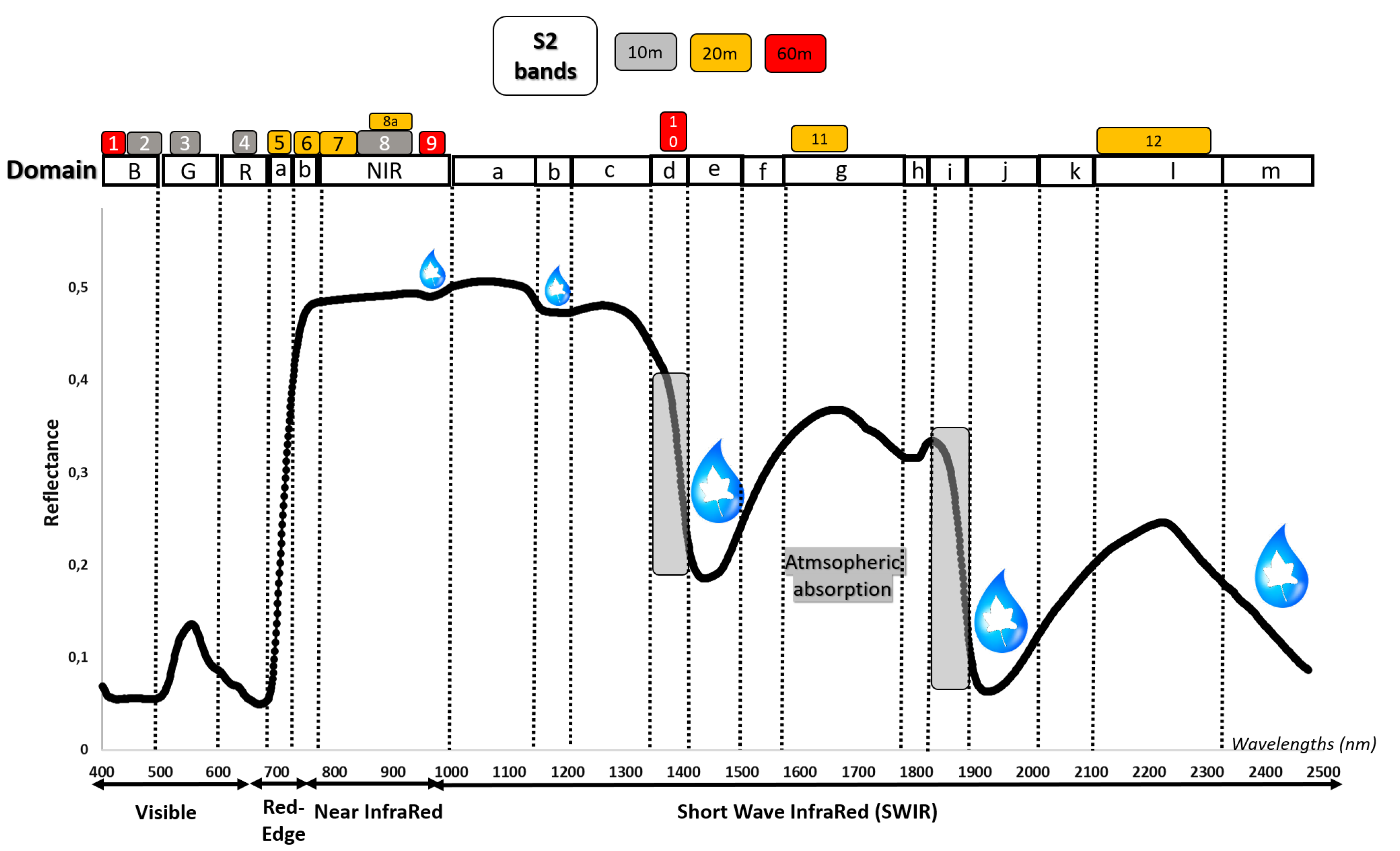
| Wavelength (nm) | Domain | Wavelength (nm) | Domain | Wavelength (nm) | Domain |
|---|---|---|---|---|---|
| 400–500 | Blue | 1131–1190 | SWIR b | 1801–1870 | SWIR i |
| 501–600 | Green | 1191–1330 | SWIR c | 1871–2000 | SWIR j |
| 601–670 | Black | 1331–1390 | SWIR d | 2001–2100 | SWIR k |
| 671–700 | Red-Edge_a | 1391–1480 | SWIR e | 2101–2310 | SWIR l |
| 701–750 | Red-Edge_b | 1481–1550 | SWIR f | 2311–2474 | SWIR m |
| 751–1000 | NIR | 1551–1760 | SWIR g | ||
| 1001–1130 | SWIR a | 1761–1800 | SWIR h |
| Index (Abbreviation) | Use | Formula Used | Reference |
|---|---|---|---|
| Normalized Difference Vegetation Index (NDVI) | Vigor | [57] | |
| Modified Chlorophyll Absorption Ratio Index/Optimized Soil Adjusted Vegetation Index (MCARI/OSAVI) | Chlorophyll | [58] | |
| Normalized difference Red-Edge (NDRE) | Chlorophyll, Water | [51] | |
| Inverted Red-Edge Chlorophyll Index (IRECI) | Chlorophyll | [59] | |
| Red-Edge Chlorophyll Absorption Index(RECAI) | Chlorophyll | [60] | |
| Normalized Difference Infrared Index(NDII) | Chlorophyll, Water | [61] | |
| Red-Edge Position (REP) | Chlorophyll | [62] | |
| Hyperspectral indices adapted to multispectral | |||
| Moisture stress Index (MSI) | Water | [56] | |
| Leaf Water Index (LWI) | Water | [36] | |
| Spectrum | Features | Number of Features |
|---|---|---|
| Raw reflectance by wavelengths | Each wavelengths | 1974 |
| NDSI | 1,947,351 | |
| HVI | 7 | |
| Reflectance average by domains | Each domain | 18 |
| NDSI | 153 | |
| MVI | 9 |
| All Data | Plots A and C | Plot B | |
|---|---|---|---|
| Variables | SWP | ||
| SWP | 1 | 1 | 1 |
| CI | 0.007 | 0.043 | 0.397 * |
| MCARI | 0.004 | 0.135 | 0.019 |
| PRI | 0.004 | 0.040 | 0.140 |
| WBI | 0.091 | <0.001 | 0.272 * |
| NDWI | 0.398 * | 0.006 | 0.258 * |
| MSI | 0.317 * | <0.001 | 0.286 * |
| LWI | 0.059 | 0.621 * | 0.047 |

| All Plots | Plots A and C | Plot B | |
|---|---|---|---|
| Variables | SWP | ||
| SWP | 1 | 1 | 1 |
| NDVI | 0.002 | 0.162 | 0.064 |
| MCARI/OSAVI | 0.007 | 0.202 | 0.002 |
| LWI | 0.109 | 0.185 | 0.475 * |
| REP | 0.003 | 0.411 * | 0.023 |
| IRECI | <0.001 | 0.307 * | 0.043 |
| RECAI | <0.001 | 0.367 * | 0.044 |
| NDII | 0.309 * | 0.244 * | <0.001 |
| MSI | 0.309 * | 0.243 * | <0.001 |
| NDRE1 | 0.004 | 0.359 * | 0.037 |
| NDRE2 | 0.002 | 0.397 * | 0.034 |

Publisher’s Note: MDPI stays neutral with regard to jurisdictional claims in published maps and institutional affiliations. |
© 2021 by the authors. Licensee MDPI, Basel, Switzerland. This article is an open access article distributed under the terms and conditions of the Creative Commons Attribution (CC BY) license (http://creativecommons.org/licenses/by/4.0/).
Share and Cite
Laroche-Pinel, E.; Albughdadi, M.; Duthoit, S.; Chéret, V.; Rousseau, J.; Clenet, H. Understanding Vine Hyperspectral Signature through Different Irrigation Plans: A First Step to Monitor Vineyard Water Status. Remote Sens. 2021, 13, 536. https://0-doi-org.brum.beds.ac.uk/10.3390/rs13030536
Laroche-Pinel E, Albughdadi M, Duthoit S, Chéret V, Rousseau J, Clenet H. Understanding Vine Hyperspectral Signature through Different Irrigation Plans: A First Step to Monitor Vineyard Water Status. Remote Sensing. 2021; 13(3):536. https://0-doi-org.brum.beds.ac.uk/10.3390/rs13030536
Chicago/Turabian StyleLaroche-Pinel, Eve, Mohanad Albughdadi, Sylvie Duthoit, Véronique Chéret, Jacques Rousseau, and Harold Clenet. 2021. "Understanding Vine Hyperspectral Signature through Different Irrigation Plans: A First Step to Monitor Vineyard Water Status" Remote Sensing 13, no. 3: 536. https://0-doi-org.brum.beds.ac.uk/10.3390/rs13030536