The Indian COSMOS Network (ICON): Validating L-Band Remote Sensing and Modelled Soil Moisture Data Products

 , , , , , , , , , ,
  , , ,
, , ,
Abstract
:
1. Introduction
2. Description of ICON
- Berambadi-BMB: The Berambadi watershed (89 km) is located in the Gundlupet taluk, Chamrajanagara district of Karnataka in South India and belongs to Kabini critical zone observatory. The Kabini Critical Zone Observatory is monitored under the project AMBHAS. The catchment has been instrumented as a Calibration and Validation (CAL/VAL) site for various satellite missions like SMOS and RISAT-1 under AMBHAS [40]. The climate in the catchment is sub-humid with annual precipitation of 800 mm and annual potential evapo-transpiration of 1539 mm based on MOD16 (MODIS global evapotranspiration data). The Köppen Climate Classification is “Aw”: Tropical Savanna climate. The soil type in the catchment comprises of red soil to black soil near valley. The major soil types in the region include sandy clay loam, sandy loam and sandy clay (see Figure 1). Average farm size in the catchment is about 1.2 hectares [40] and about 60% of land is under ground water irrigation and 40% is rain fed. The major crops in the catchment are turmeric, sunflower, maize, marigold and vegetables. The main crop in the catchment is grown during Kharif season (May to September). Rabi crop (October to December) and summer crop (January to April) is practiced in case if the farmer has access to irrigation [41]. Site is equipped with flux towers at 10 m height. Weather parameters like global radiation, wind speed, relative humidity and rainfall are monitored in the tower. SM (Stevens Hydra Probe and COSMOS), ground water fluctuation and crop dynamics (LAI and crop type) are monitored in the site.
- Madahalli-MDH: Madahalli microwatershed is located in Gundlupet taluk of Chamrajanagara district close to the BMB site. It is an agricultural area. The climate in the region is semi-arid and the annual precipitation is about 734 mm and annual PET is 1530 mm (MOD16). The major crop in the area include ragi, sunflower, red gram, maize and vegetables. Groundwater irrigation is practiced in the catchment. The Köppen Climate Classification is “Aw”. The weather variables are measured using flux tower. SM at point scale is monitored using Stevens Hydra Probe and at field scale is monitored using COSMOS sensor. Crop monitoring and ground water level monitoring is also carried out in the sites.
- Singanallur-SGR: Singanallur watershed is located in Kollegala Taluk of Chamarajanagara district in the southern part of Karnataka state. The annual rainfall in the area is found to be 780 mm. The potential evapotranspiration in the region is 1476 mm based on MOD16 data. It is an agricultural area. The major crops grown in the region are vegetables, sunflower, ragi and maize [42]. The Köppen Climate Classification is “Aw”: Tropical Savanna climate. Weather variables, crop monitoring and ground water level monitoring is carried out. SM is monitored using Stevens Hydra Probe and COSMOS.
- Dharwad-DWD: Dharwad is situated in northern part of Karnataka state which is in south Indian region with annual rainfall of about 761 mm and min temp 20 °C and max temperature being 35 °C. The potential evapotranspiration in the region 1639 mm (MOD16). The major soil type in the region is vertisol. The area is under University of Agricultural Science (UAS) Dharwad, and is mainly used for scientific studies in the agricultural sector. The major crops grown in the area are cotton, jowar, maize, wheat, rice etc. Surface water irrigation is practiced in the region (District Irrigation Plan). The Köppen Climate Classification is “Bsh”: Hot semi-arid climate. Weather variables are collected in the site.
- Pune-PNE: Pune is located in the central part of India in Maharashtra state. COSMOS is located inside the campus of Indian Institute of Tropical Meteorology (IITM) and is mostly covered by vegetation with sparse trees (see Figure 1). The major soil type in the area is sandy clay loam. The annual average rainfall is about 650 mm. The potential evapotranspiration in the region 1699 mm (MOD16). The Köppen Climate Classification is “Am”: Tropical monsoon climate. The site belongs to Indian Institute of Tropical Meteorology, Pune and is majorly used for scientific research. The COSMOS sensor is located in the middle of natural vegetation with shrubs and some small trees to around 4 to 6 m height. The field SM monitored using COSMOS.
- Kanpur-KPR: Kanpur is located in northern part of India in Uttar pradesh state with average annual rainfall of 650 mm. The soil type in the region is fluvisol (silty loam) [43]. The potential evapotranspiration in the region 1700 mm (MOD16). The Köppen Climate Classification is “Cwa”: Humid subtropical climate. COSMOS is located in an agricultural area maintained by Indian Institute of Technology, Kanpur which is majorly used for scientific purposes. The site is in an area with sparse trees adjacent to agricultural plots, and at 2 km to dense urban areas. Weather variables in the site are collected using flux station.
- Henval-HNL: Henval Valley is located near Chamba town in the Uttarakhand state in northern India with minimum temperature of 1.1 °C and max temperature of 32.9 °C. The site is situated on the banks of Henval river. The major soil types in the region are sandy loam, loam and sandy clay loam. Annual average rainfall is about 1120 mm. The potential evapotranspiration in the region 1791 mm (MOD16). Irrigation in the region is either done by tapping spring water or by using surface water.The Köppen Climate Classification is “Cwa”: Humid subtropical climate.
3. Spatial Soil Moisture Datasets
3.1. Satellite Data
3.1.1. Soil Moisture and Ocean Salinity Satellite (SMOS) Data
3.1.2. Soil Moisture Active Passive (SMAP) Data
3.2. Land Surface Model
4. Methodology
4.1. Calibration of the COSMOS
4.2. Evaluation Metrics
- RMSE: Root Mean Squared Errorwhere, E[.] is expectation operator. is the SM from spatial products, and is ICON-COSMOS soil moisture.
- R: Pearson’s correlation coefficientwhere and are variances of time series of and respectively.
- Bias
- ubRMSE: Unbiased RMSE
5. Results
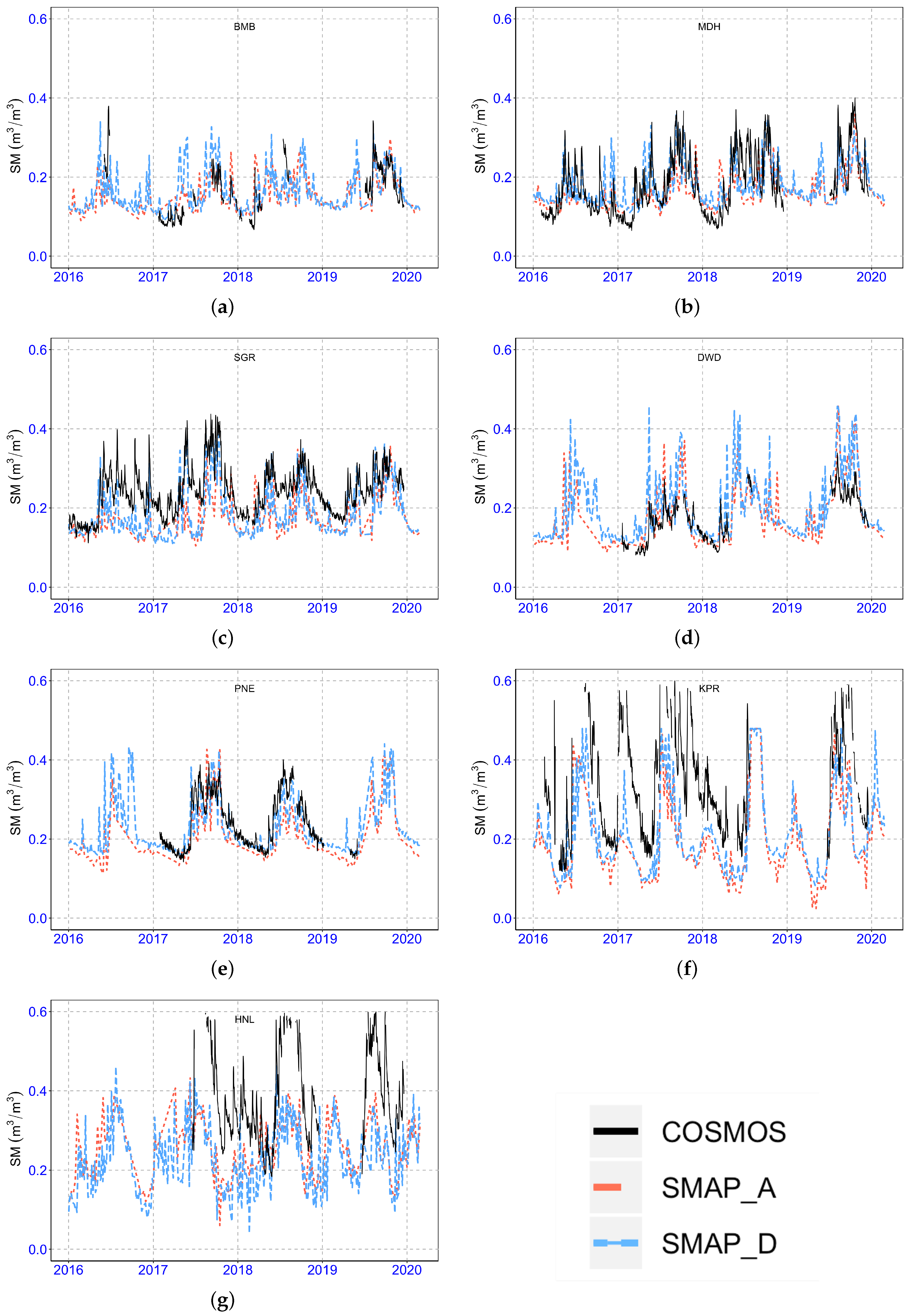
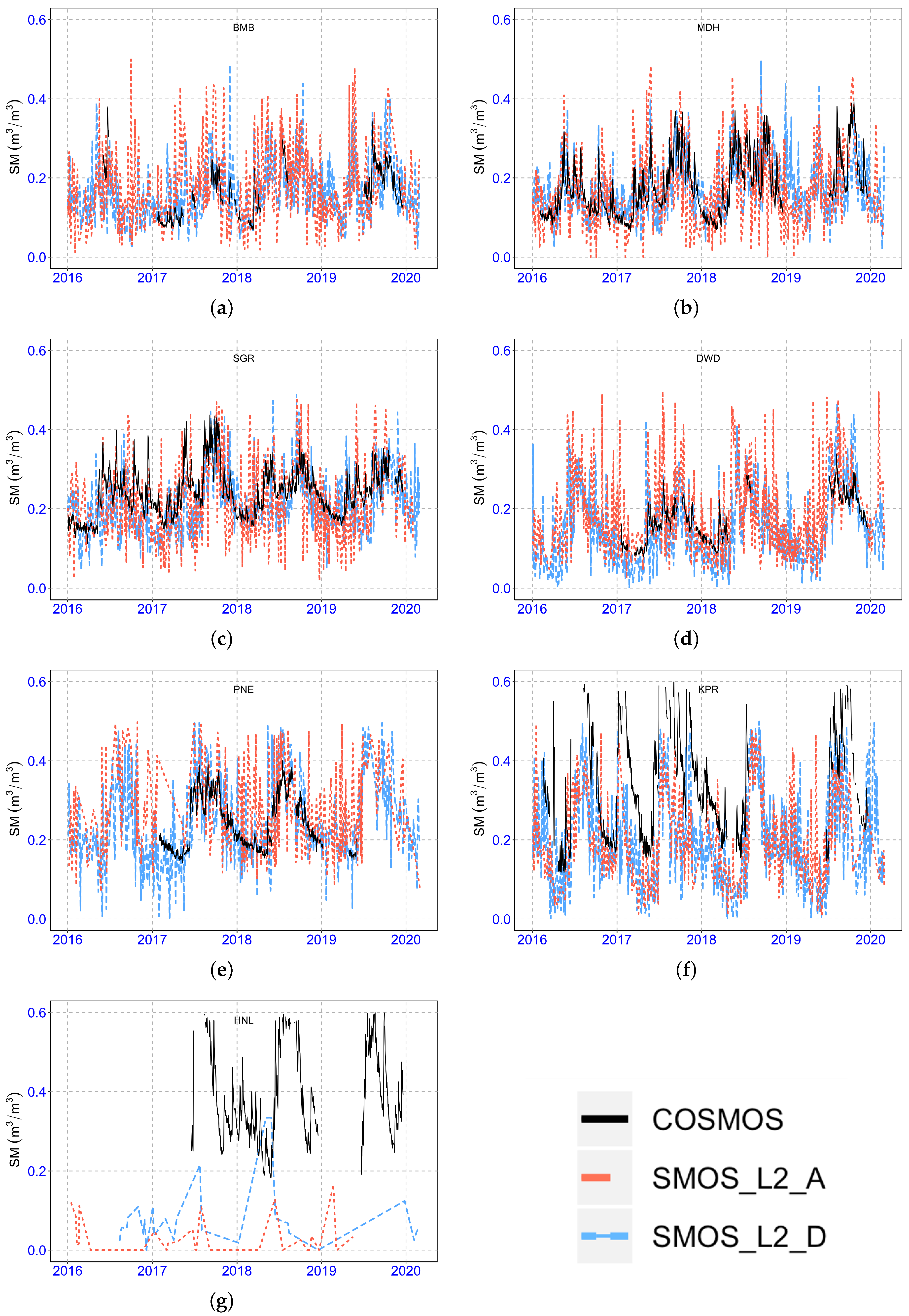
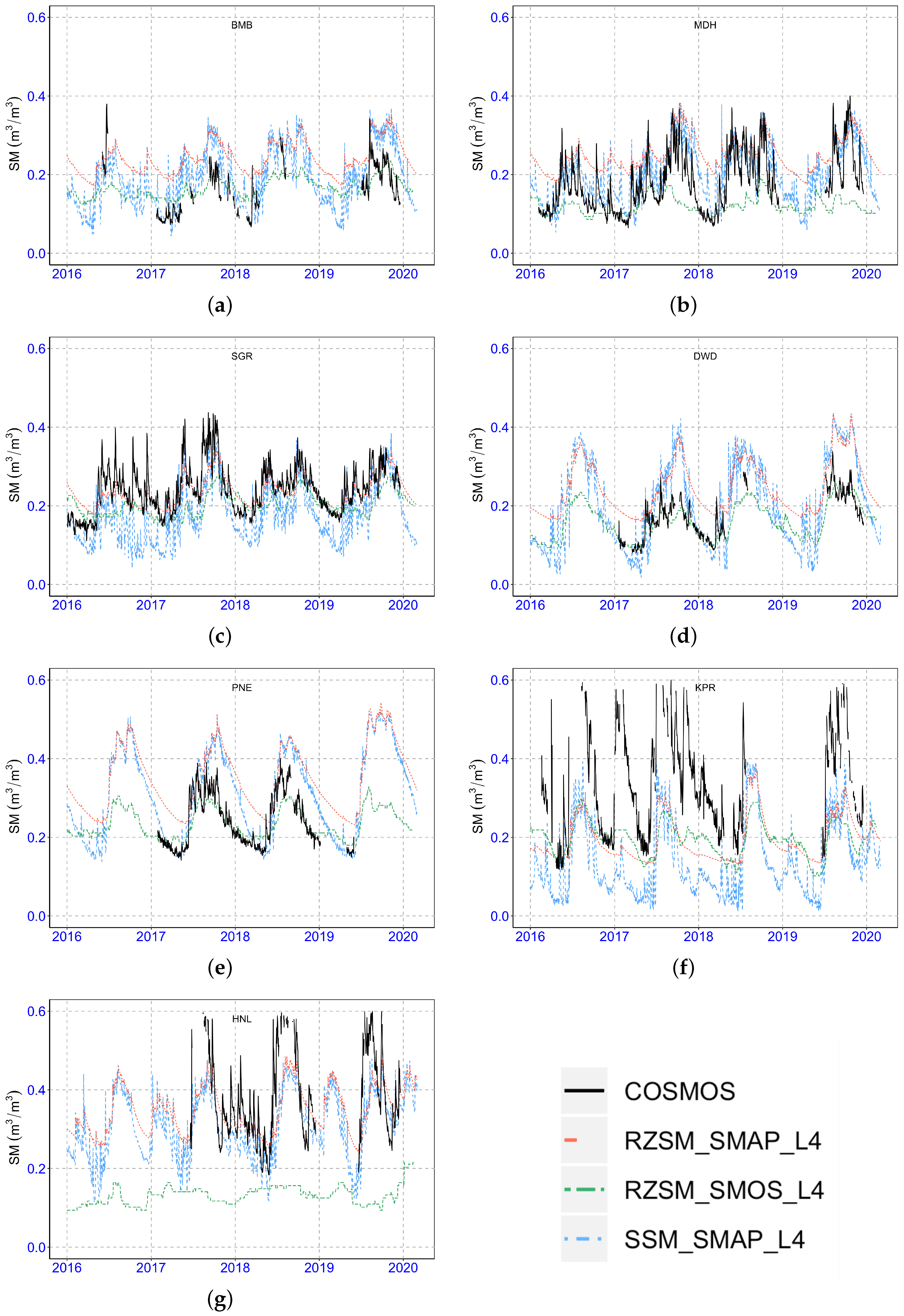
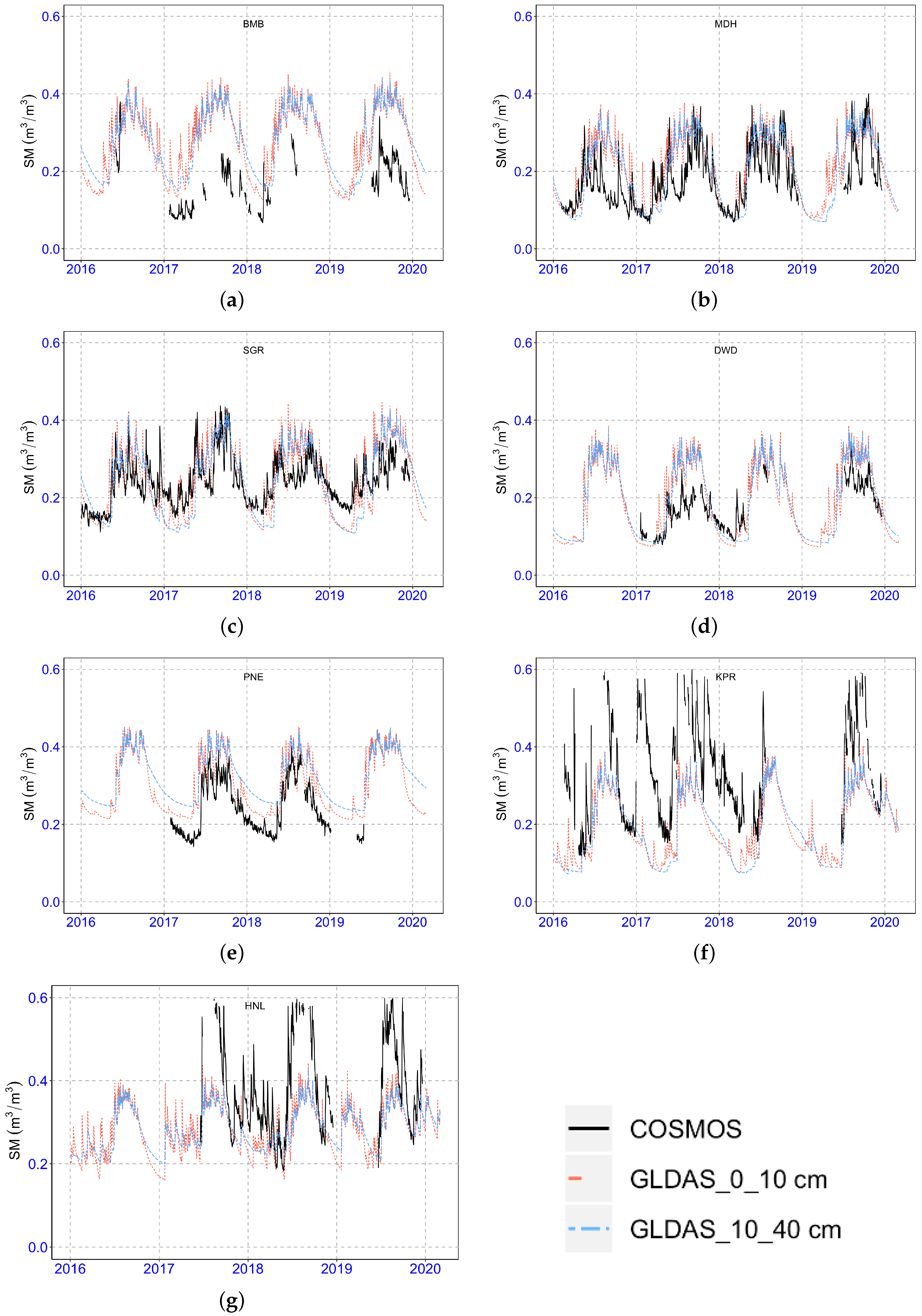
- Berambadi-BMB: COSMOS SM time series (see Figure 6a) over BMB show high fluctuations during crop growth season, which can be explained by the impact of irrigation as the instrument is installed in a groundwater irrigated agricultural plot. The mean, maximum and minimum COSMOS SM over this site are 0.16 (m/m), 0.42 (m/m) and 0.07 (m/m), respectively. SM in Berambadi from different satellite and GLDAS products showed R values of 0.62, 0.66, 0.41, 0.52 and 0.76 for SMAP_L3_A, SMAP_L3_D, SMOS_L2_A, SMOS_L2_D and GLDAS respectively. The performance of GLDAS shows the best results, followed by SMAP and then SMOS products. Comparison of COSMOS with GLDAS RZSM data set (see Figure 6a) shows R values of 0.76, 0.77, 0.73 and 0.69 for (0–10 cm), (10–40 cm), (40–100 cm) and (100–200 cm) respectively. The performances for first and second layers are similar. For deeper layers the correlation decreases significantly. In the case of SSM and RZSM from SMAP the R values were of 0.8 and 0.72 respectively. The RZSM from SMOS_L4 shows R value of 0.67. The SSM has a significantly higher correlation (see Figure 5a).
- Madahalli-MDH: COSMOS sensor located in Madahalli site is also in an agricultural field (see Figure 1). The site is close to the Berambadi site. The mean, maximum and minimum SM from COSMOS sensor are 0.18 (m/m), 0.40 (m/m) and 0.065 (m/m) which very close to the Berambadi site. SM comparison with different SSM products SMAP_L3_A, SMAP_L3_D, SMOS_L2_A, SMOS_L2_D and GLDAS shows R value of 0.73, 0.76, 0.52 0.62 and 0.70 respectively. This shows the product SMAP_L3_D and GLDAS are performing equally well in this site for SM comparison (see Table 4). RZSM analysis shows that for GLDAS product at (0–10 cm), (10–40 cm), (40–100 cm) and (100–200 cm) shows R values of 0.7, 0.69, 0.61 and 0.6 respectively (see Figure 6. In Madahalli site the best performance is obtained like for BMB at (0–10 cm) and (10–40 cm) depths. For SMAP_L4 product R value was of 0.8 and 0.72 for SSM and RZSM respectively, showing significantly better performances for SSM (see Figure 5b). SMOS_L4 RZSM showed R value of 0.54 which is significantly less compared to SMAP_L4.
- Singanallur-SGR: Singanallur site is an irrigated agricultural plot (see Figure 1) with mean, maximum and minimum SM from COSMOS of 0.244 (m/m), 0.44 (m/m) and 0.11 (m/m), respectively. The higher mean value is consistent with the fact that this soil in the site has a higher percentage of clay than the Berambadi and Madahalli sites (see Figure 1). SSM from SMAP_L3_A, SMAP_L3_D, SMOS_L2_A, SMOS_L2_D and GLDAS show values of R 0.71, 0.81, 0.42, 0.52 and 0.78 respectively (see Table 4). From the values in the Table 5 and Table 6 it can be seen that the performance of SMAP_L4 SSM and GLDAS are giving best performance (see Figure 5 and Figure 6). The RZSM from GLDAS at (0–10 cm), (10–40 cm), (40–100 cm) and (100–200 cm) shows R values of 0.78, 0.71, 0.58 and 0.5 respectively, (see Figure 6c) showing close results for (0–10 cm) and (10–40 cm) depth. The COSMOS value is comparable to 0–40 cm from GLDAS product with good performance. The SMAP_L4 SSM and RZSM comparison shows values of R as 0.81 and 0.74, respectively (see Figure 5c), which is close to GLDAS performance.SMOS_L4 RZSM shows R value of 0.42 which is lower as compared to SMAP_L4 and GLDAS products.
- Dharwad-DWD: The COSMOS data time series shows a mean value of 0.17, maximum of 0.34 and minimum of 0.08 (m/m), respectively. SMAP_L3_A (R = 0.87) outperforms other products followed by GLDAS (R = 0.82) then SMAP_L3_D (R = 0.82) then SMOS_L2_D (R = 0.79) and SMOS_L2_A (R = 0.66) (see Table 4). All SSM products have good performances over this site. The RZSM comparison between GLDAS products and COSMOS (see Figure 6d) showed best comparison at all depths indicating minor differences in soil moisture across depths. The performance at all depths showed higher R values 0.82, 0.85, 0.85 and 0.84 respectively at depths (0–10 cm), (10–40 cm), (40–100 cm) and (100–200 cm) (see Table 6). Comparison of RZSM from SMAP_L4 and COSMOS (see Figure 5d) products showed better results at top layer with R value of 0.9 compared to deeper (R = 0.86) and from SMOS_L4 showed R value of 0.89 close to SMAP_L4.
- Pune-PNE: The site is located in a vegetated cover with sparse trees. The mean COSMOS SM value was 0.238 (m/m), maximum was 0.404 (m/m) and minimum 0.142 (m/m). The higher mean and minimum value can be attributed to the presence of sparse trees that preserve the soil moisture combined to the higher percentage clay in this site (see Figure 1). Over this site the SSM performance of GLDAS (R = 0.89) is best followed by SMAP_L3_D (R = 0.88) then by SMAP_L3_A (R = 0.83), SMOS_L2_D (R = 0.74), SMOS_L2_A (R = 0.50) (see Table 4). The RZSM data comparison between GLDAS and COSMOS (see Figure 6e) is showing very good performance at all depth with best performance at depth 10–40 cm with R value of 0.94. Comparison with SMAP_L4 and COSMOS (see Figure 5e) data showed better performance at top layer (R = 0.83) in comparison to the deeper layer (R = 0.75). Comparison of COSMOS with SMOS_L4 showed R value of 0.89.
- Kanpur-KPR: The comparison of SM from COSMOS sensor to spatial SM at the Kanpur site poses several challenges, the sensor is a non-representative area in a rice field with high dense urban areas (25% of the satellite footprint). The maximum value of soil moisture reported in this site reaches extremely high values above soil saturation (>0.50 (m/m)) because of standing water and was filtered out. The minimum is 0.117 (m/m) and the average 0.40 (m/m). The effect of irrigation is captured in the COSMOS measurements and not by any other products considered in the study indicated by peaks in COSMOS data when compared to products. All products show high bias that is explained by the reasons presented above, in fact the impact of urban areas is similar to bare rocks and induces negative bias in the retrieved SM. SMOS data shows some outliers (see Figure 3f). The performance of SMAP_L3_A (R = 0.89) shows the best performance followed by SMAP_L3_D (R = 0.82) then SMOS_L2_A (R = 0.71), SMOS_L2_D (R = 0.68) and then GLDAS (R = 0.63) (see Table 4). This shows that urban areas impacts the bias of the retrievals and to a much lesser extent the correlation as the urban environment is static bare rocks in passive microwave. This is true provided that zero to low levels of RFIs are from the urban environment. The RZSM comparison with GLDAS and COSMOS (see Figure 6f) showed best performance at depths 0–10 cm and 10–40 cm. The R values were 0.63 and 0.62 respectively. Comparison of SMAP_L4 and COSMOS (see Figure 5f) showed better R values for top layer as compared to deeper layer (0.79 and 0.74 respectively). Comparison of COSMOS with SMOS_L4 show R value of 0.66.
- Henval-HNL: The time series of COSMOS SM at the site has a mean value of 0.416 (m/m), maximum of 0.812 (m/m), and minimum of 0.183 (m/m). These high values are expected as the site is in a subtropical humid region in the Himalayas with 1120 mm/y of rainfall. Moreover the site is situated in a high altitude valley that experiences snow melting (see Figure 1). Rice cultivation is practiced in plots in the footprint of the COSMOS sensor and periodic irrigation for rice crops is seen. The local irrigation effect is very well captured in the COSMOS measurements and is not reflected to the same extent in the spatial products. This can be explained by the relatively small surface cover of the agricultural area when compared to the footprint of the satellite data. It is also worth mentioning that the site is located over mountainous region that impacts the SM retrieval in microwave. The performance of GLDAS (R = 0.75), SMAP_L3_A (R = 0.73) and SMAP_L3_D (R = 0.74) shows similar results with slight variations (see Table 4). SMOS data is not valid for this site (see Figure 3g) due to very high levels of RFIs and high topographic index. The RZSM comparison between GLDAS and COSMOS (see Figure 6g) showed better performance at depth of 10–40 cm. The R values at depths (0–10 cm), (10–40 cm), (40–100 cm) and (100–200 cm) show 0.75, 0.78, 0.62 and 0.26 respectively. Comparison with SMAP_L4 data and COSMOS data showed better result for top layer with R value of 0.76 in comparison to deeper layer which reported 0.66 R value (see Figure 5g).
6. Discussions
6.1. Surface and Root-Zone SM versus COSMOS Measurements
6.2. Performances with Respect to Soil Properties and Climate Information
6.3. Matching In Situ and Satellite Data Footprint
7. Conclusions
Supplementary Materials
Author Contributions
Funding
Institutional Review Board Statement
Informed Consent Statement
Data Availability Statement
Acknowledgments
Conflicts of Interest
Abbreviations
| SM | Soil Moisture |
| SSM | Surface Soil Moisture |
| RZSM | Root Zone Soil Moisture |
| ICON | Indian COSMOS Network |
| AMBHAS | Assimilation of Multi-satellite data at Berambadi watershed for Hydrology |
| And land Surface experiment | |
| NAFE | The National Airborne Field Experiment |
| SMAPEX | Soil Moisture Active Passive Experiment |
| SGP | The Southern Great Plains |
| ICOS | Integrated Carbon Obervation Network |
| ISMN | International Soil Moisture Network |
| MDPI | Multidisciplinary Digital Publishing Institute |
| CRNP | Cosmic Ray Neutron Probe |
| COSMOS | COsmic ray Soil Moisture Observation System |
| SMOS | Soil Moisture Observation System |
| SMAP | Soil Moisture Active Passive |
| GLDAS | Global Land Data Assimilation System |
| ASCAT | Advanced Scatterometer |
| AMSR | Advanced Microwave Scanning Radiometer |
| LSM | Land Surface Modelling |
| KSNDMC | Karnataka State Natural and Disaster Mangement Centre |
| TB | Brightness Temperature |
| NASA | National Aeronautics and Space Administration |
| ISRO | Indian Space Research Organisation |
| NISAR | NASA-ISRO Synthetic Aperture Radar mission |
| RFI | Radio Frequency Interference |
References
- Evans, J.G.; Ward, H.C.; Blake, J.R.; Hewitt, E.J.; Morrison, R.; Fry, M.; Ball, L.A.; Doughty, L.C.; Libre, J.W.; Hitt, O.E.; et al. Soil water content in southern England derived from a cosmic-ray soil moisture observing system—COSMOS-UK. Hydrol. Process. 2016, 30, 4987–4999. [Google Scholar] [CrossRef] [Green Version]
- Bojinski, S.; Verstraete, M.; Peterson, T.C.; Richter, C.; Simmons, A.; Zemp, M. The concept of essential climate variables in support of climate research, applications, and policy. Bull. Am. Meteorol. Soc. 2014, 95, 1431–1443. [Google Scholar] [CrossRef]
- Fereres, E.; Soriano, M.A. Deficit irrigation for reducing agricultural water use. J. Exp. Bot. 2007, 58, 147–159. [Google Scholar] [CrossRef] [PubMed] [Green Version]
- Komma, J.; Blöschl, G.; Reszler, C. Soil moisture updating by Ensemble Kalman Filtering in real-time flood forecasting. J. Hydrol. 2008, 357, 228–242. [Google Scholar] [CrossRef]
- Fan, L.; Wigneron, J.P.; Xiao, Q.; Al-Yaari, A.; Wen, J.; Martin-StPaul, N.; Dupuy, J.L.; Pimont, F.; Al Bitar, A.; Fernandez-Moran, R.; et al. Evaluation of microwave remote sensing for monitoring live fuel moisture content in the Mediterranean region. Remote Sens. Environ. 2018, 205, 210–223. [Google Scholar] [CrossRef]
- Pelletier, J.D. Scale-invariance of soil moisture variability and its implications for the frequency-size distribution of landslides. arXiv 1997, arXiv:physics/9705035. [Google Scholar] [CrossRef]
- Hendrickx, J.M.; Harrison, J.B.J.; Borchers, B.; Kelley, J.R.; Howington, S.; Ballard, J. High-resolution soil moisture mapping in Afghanistan. In Detection and Sensing of Mines, Explosive Objects, and Obscured Targets XVI; International Society for Optics and Photonics: Orlando, FL, USA, 2011; Volume 8017, p. 801710. [Google Scholar]
- Karthikeyan, L.; Chawla, I.; Mishra, A.K. A review of remote sensing applications in agriculture for food security: Crop growth and yield, irrigation, and crop losses. J. Hydrol. 2020, 586, 124905. [Google Scholar] [CrossRef]
- SU, S.L.; Singh, D.; Baghini, M.S. A critical review of soil moisture measurement. Measurement 2014, 54, 92–105. [Google Scholar] [CrossRef]
- Rodriguez-Alvarez, N.; Bosch-Lluis, X.; Camps, A.; Vall-Llossera, M.; Valencia, E.; Marchan-Hernandez, J.F.; Ramos-Perez, I. Soil moisture retrieval using GNSS-R techniques: Experimental results over a bare soil field. IEEE Trans. Geosci. Remote Sens. 2009, 47, 3616–3624. [Google Scholar] [CrossRef]
- Acevo-Herrera, R.; Aguasca, A.; Bosch-Lluis, X.; Camps, A. On the use of compact L-band Dicke radiometer (ARIEL) and UAV for soil moisture and salinity map retrieval: 2008/2009 field experiments. In Proceedings of the 2009 IEEE International Geoscience and Remote Sensing Symposium, Cape Town, South Africa, 12–17 July 2009; Volume 4, pp. IV-729–IV-732. [Google Scholar]
- Zreda, M.; Shuttleworth, W.J.; Zeng, X.; Zweck, C.; Desilets, D.; Franz, T.; Rosolem, R. COSMOS: The cosmic-ray soil moisture observing system. Hydrol. Earth Syst. Sci. 2012, 16, 4079–4099. [Google Scholar] [CrossRef] [Green Version]
- Bogena, H.R.; Huisman, J.A.; Güntner, A.; Hübner, C.; Kusche, J.; Jonard, F.; Vey, S.; Vereecken, H. Emerging methods for noninvasive sensing of soil moisture dynamics from field to catchment scale: A review. Wiley Interdiscip. Rev. Water 2015, 2, 635–647. [Google Scholar] [CrossRef] [Green Version]
- Kohli, M.; Schron, M.; Zreda, M.; Schmidt, U.; Dietrich, P.; Zacharias, S. Footprint characteristics revised for field-scale soil moisture monitoring with cosmic-ray neutrons. J. Am. Water Resour. Assoc. 2015, 5, 5772–5790. [Google Scholar] [CrossRef] [Green Version]
- Baatz, R.; Bogena, H.; Franssen, H.J.H.; Huisman, J.A.; Montzka, C.; Vereecken, H. An empirical vegetation correction for soil water content quantification using cosmic ray probes. Water Resour. Res. 2015, 51, 2030–2046. [Google Scholar] [CrossRef] [Green Version]
- Dorigo, W.; Wagner, W.; Hohensinn, R.; Hahn, S.; Paulik, C.; Xaver, A.; Gruber, A.; Drusch, M.; Mecklenburg, S.; van Oevelen, P.; et al. The International Soil Moisture Network: A data hosting facility for global in situ soil moisture measurements. Hydrol. Earth Syst. Sci. 2011, 15, 1675–1698. [Google Scholar] [CrossRef] [Green Version]
- Brocca, L.; Morbidelli, R.; Melone, F.; Moramarco, T. Soil moisture spatial variability in experimental areas of central Italy. J. Hydrol. 2007, 333, 356–373. [Google Scholar] [CrossRef]
- Albergel, C.; de Rosnay, P.; Gruhier, C.; Muñoz-Sabater, J.; Hasenauer, S.; Isaksen, L.; Kerr, Y.; Wagner, W. Evaluation of remotely sensed and modelled soil moisture products using global ground-based in situ observations. Remote Sens. Environ. 2012, 118, 215–226. [Google Scholar] [CrossRef]
- Kerr, Y.H.; Waldteufel, P.; Wigneron, J.P.; Delwart, S.; Cabot, F.; Boutin, J.; Escorihuela, M.J.; Font, J.; Reul, N.; Gruhier, C.; et al. The SMOS mission: New tool for monitoring key elements ofthe global water cycle. Proc. IEEE 2010, 98, 666–687. [Google Scholar] [CrossRef] [Green Version]
- Entekhabi, B.D.; Njoku, E.G.; Neill, P.E.O.; Kellogg, K.H.; Crow, W.T.; Edelstein, W.N.; Entin, J.K.; Goodman, S.D.; Jackson, T.J.; Johnson, J.; et al. The Soil Moisture Active and Passive (SMAP) mission. Proc. IEEE 2010, 98, 704–716. [Google Scholar] [CrossRef]
- Bartalis, Z.; Wagner, W.; Naeimi, V.; Hasenauer, S.; Scipal, K.; Bonekamp, H.; Figa, J.; Anderson, C. Initial soil moisture retrievals from the METOP-A Advanced Scatterometer (ASCAT). Geophys. Res. Lett. 2007, 34, 5–9. [Google Scholar] [CrossRef] [Green Version]
- Parinussa, R.M.; Holmes, T.R.; Wanders, N.; Dorigo, W.A.; De Jeu, R.A. A preliminary study toward consistent soil moisture from AMSR2. J. Hydrometeorol. 2015, 16, 932–947. [Google Scholar] [CrossRef]
- Tomer, S.; Al Bitar, A.; Sekhar, M.; Zribi, M.; Bandyopadhyay, S.; Kerr, Y. MAPSM: A spatio-temporal algorithm for merging soil moisture from active and passive microwave remote sensing. Remote Sens. 2016, 8, 990. [Google Scholar] [CrossRef] [Green Version]
- Chakravorty, A.; Chahar, B.R.; Sharma, O.P.; Dhanya, C.T. A regional scale performance evaluation of SMOS and ESA-CCI soil moisture products over India with simulated soil moisture from MERRA-Land. Remote Sens. Environ. 2016, 186, 514–527. [Google Scholar] [CrossRef]
- Suman, S.; Srivastava, P.K.; Petropoulos, G.P.; Pandey, D.K.; O’Neill, P.E. Appraisal of SMAP operational soil moisture product from a global perspective. Remote Sens. 2020, 12, 1977. [Google Scholar] [CrossRef]
- Attada, R.; Kumar, P.; Dasari, H.P. Assessment of Land Surface Models in a High-Resolution Atmospheric Model during Indian Summer Monsoon. Pure Appl. Geophys. 2018, 175, 3671–3696. [Google Scholar] [CrossRef] [Green Version]
- Bindlish, R.; Jackson, T.J.; Gasiewski, A.J.; Klein, M.; Njoku, E.G. Soil moisture mapping and AMSR-E validation using the PSR in SMEX02. Remote Sens. Environ. 2006, 103, 127–139. [Google Scholar] [CrossRef]
- Bosch, D.D.; Lakshmi, V.; Jackson, T.J.; Choi, M.; Jacobs, J.M. Large scale measurements of soil moisture for validation of remotely sensed data: Georgia soil moisture experiment of 2003. J. Hydrol. 2006, 323, 120–137. [Google Scholar] [CrossRef]
- Al Bitar, A.; Leroux, D.; Kerr, Y.H.; Merlin, O.; Richaume, P.; Sahoo, A.; Wood, E.F. Evaluation of SMOS soil moisture products over continental US using the SCAN/SNOTEL network. IEEE Trans. Geosci. Remote Sens. 2012, 50, 1572–1586. [Google Scholar] [CrossRef] [Green Version]
- Merlin, O.; Rüdiger, C.; Al Bitar, A.; Richaume, P.; Walker, J.P.; Kerr, Y.H. Disaggregation of SMOS soil moisture in Southeastern Australia. IEEE Trans. Geosci. Remote Sens. 2012, 50, 1556–1571. [Google Scholar] [CrossRef] [Green Version]
- Montzka, C.; Bogena, H.R.; Weihermüller, L.; Jonard, F.; Bouzinac, C.; Kainulainen, J.; Balling, J.E.; Loew, A.; Dall’Amico, J.T.; Rouhe, E.; et al. Brightness temperature and soil moisture validation at different scales during the SMOS validation campaign in the Rur and Erft catchments, Germany. IEEE Trans. Geosci. Remote Sens. 2013, 51, 1728–1743. [Google Scholar] [CrossRef]
- Dente, L.; Su, Z.; Wen, J. Validation of SMOS soil moisture products over the Maqu and Twente Regions. Sensors 2012, 12, 9965–9986. [Google Scholar] [CrossRef]
- Al-Yaari, A.; Wigneron, J.P.; Ducharne, A.; Kerr, Y.; Wagner, W.; De Lannoy, G.; Reichle, R.; Al Bitar, A.; Dorigo, W.; Richaume, P.; et al. Global-scale comparison of passive (SMOS) and active (ASCAT) satellite based microwave soil moisture retrievals with soil moisture simulations (MERRA-Land). Remote Sens. Environ. 2014, 152, 614–626. [Google Scholar] [CrossRef] [Green Version]
- Colliander, A.; Jackson, T.J.; Bindlish, R.; Chan, S.; Das, N.; Kim, S.B.; Cosh, M.H.; Dunbar, R.S.; Dang, L.; Pashaian, L.; et al. Validation of SMAP surface soil moisture products with core validation sites. Remote Sens. Environ. 2017, 191, 215–231. [Google Scholar] [CrossRef]
- Gruber, A.; Dorigo, W.; Zwieback, S.; Xaver, A.; Wagner, W. Characterizing Coarse-Scale Representativeness of in situ Soil Moisture Measurements from the International Soil Moisture Network. Vadose Zone J. 2013, 12, vzj2012.0170. [Google Scholar] [CrossRef] [Green Version]
- Montzka, C.; Bogena, H.R.; Zreda, M.; Monerris, A.; Morrison, R.; Muddu, S.; Vereecken, H. Validation of spaceborne and modelled surface soil moisture products with Cosmic-Ray Neutron Probes. Remote Sens. 2017, 9, 103. [Google Scholar] [CrossRef] [Green Version]
- Kȩdzior, M.; Zawadzki, J. Comparative study of soil moisture estimations from SMOS satellite mission, GLDAS database, and cosmic-ray neutrons measurements at COSMOS station in Eastern Poland. Geoderma 2016, 283, 21–31. [Google Scholar] [CrossRef]
- Kim, S.; Liu, Y.Y.; Johnson, F.M.; Parinussa, R.M.; Sharma, A. A global comparison of alternate AMSR2 soil moisture products: Why do they differ? Remote Sens. Environ. 2015, 161, 43–62. [Google Scholar] [CrossRef]
- Tomer, S.; Al Bitar, A.; Sekhar, M.; Zribi, M.; Bandyopadhyay, S.; Sreelash, K.; Sharma, A.K.; Corgne, S.; Kerr, Y. Retrieval and multi-scale validation of soil moisture from multi-temporal SAR data in a semi-arid tropical region. Remote Sens. 2015, 7, 8128–8153. [Google Scholar] [CrossRef] [Green Version]
- Sharma, A.K.; Hubert-Moy, L.; Buvaneshwari, S.; Sekhar, M.; Ruiz, L.; Bandyopadhyay, S.; Corgne, S. Irrigation history estimation using multitemporal landsat satellite images: Application to an intensive groundwater irrigated agricultural watershed in India. Remote Sens. 2018, 10, 893. [Google Scholar] [CrossRef] [Green Version]
- Robert, M.; Thomas, A.; Sekhar, M.; Badiger, S.; Ruiz, L.; Willaume, M.; Leenhardt, D.; Bergez, J.E. Farm typology in the Berambadi Watershed (India): Farming systems are determined by farm size and access to groundwater. Water 2017, 9, 51. [Google Scholar] [CrossRef] [Green Version]
- Vasundhara, R.; Dharumarajan, S.; Hegde, R.; Srinivas, S.; Niranjana, K.V.; Srinivasan, N.; Singh, S.K. Characterization and Evaluation of Soils of Singanallur Watershed Using Remote Sensing and GIS. Int. J. Bio-resour. Stress Manag. 2017, 8, 51–56. [Google Scholar] [CrossRef] [Green Version]
- Adla, S.; Rai, N.K.; Karumanchi, S.H.; Tripathi, S.; Disse, M.; Pande, S. Laboratory calibration and performance evaluation of low-cost capacitive and very low-cost resistive soil moisture sensors. Sensors 2020, 20, 363. [Google Scholar] [CrossRef] [Green Version]
- Hallikainen, M.; Winebrenner, D.P. The physical basis for sea ice remote sensing. In Geophysical Monograph Series; Carsey, F.D., Ed.; American Geophysical Union: Washington, DC, USA, 1992; Volume 68, pp. 29–46. [Google Scholar] [CrossRef]
- Moran, M.S.; Peters-Lidard, C.D.; Watts, J.M.; McElroy, S. Estimating soil moisture at the watershed scale with satellite-based radar and land surface models. Can. J. Remote Sens. 2004, 30, 805–826. [Google Scholar] [CrossRef] [Green Version]
- Njoku, E.G.; Entekhabi, D. Passive microwave remote sensing of soil moisture. J. Hydrol. 1996, 184, 101–129. [Google Scholar] [CrossRef]
- Kerr, Y.H.; Waldteufel, P.; Richaume, P.; Wigneron, J.P.; Ferrazzoli, P.; Mahmoodi, A.; Al Bitar, A.; Cabot, F.; Gruhier, C.; Juglea, S.E.; et al. The SMOS Soil Moisture Retrieval Algorithm. IEEE Trans. Geosci. Remote Sens. 2012, 50, 1384–1403. [Google Scholar] [CrossRef]
- Ahmad, A.B.; Ali, M. Algorithm Theoretical Basis Document (ATBD) for the SMOS Level 4 Root Zone Soil Moisture; Version v30_01, Zenodo 2020. Available online: https://zenodo.org/record/4298572#.YAqUhYsRXIU (accessed on 4 December 2020).
- O’Neill, P.; Chan, S.; Bindlish, R.; Jackson, T.; Colliander, A.; Dunbar, S.; Chen, F.; Piepmeier, J.; Yueh, S.; Entekhabi, D.; et al. Assessment of version 4 of the SMAP passive soil moisture standard product. Int. Geosci. Remote Sens. Symp. (IGARSS) 2017, 2017, 3941–3944. [Google Scholar] [CrossRef] [Green Version]
- Reichle, R.H.; Koster, R.D.; Dong, J.; Berg, A.A. Global soil moisture from satellite observations, land surface models, and ground data: Implications for data assimilation. J. Hydrometeorol. 2004, 5, 430–442. [Google Scholar] [CrossRef]
- Rodell, M.; Houser, P.R.; Jambor, U.; Gottschalck, J.; Mitchell, K.; Meng, C.J.; Arsenault, K.; Cosgrove, B.; Radakovich, J.; Bosilovich, M.; et al. The Global Land Data Assimilation System. Bull. Am. Meteorol. Soc. 2004, 85, 381–394. [Google Scholar] [CrossRef] [Green Version]
- Desilets, D.; Zreda, M.; Ferré, T.P. Nature’s neutron probe: Land surface hydrology at an elusive scale with cosmic rays. Water Resour. Res. 2010, 46, 1–7. [Google Scholar] [CrossRef]
- Liu, Y.; Yang, Y.; Yue, X. Evaluation of satellite-based soil moisture products over four different continental in-situmeasurements. Remote Sens. 2018, 10, 1161. [Google Scholar] [CrossRef] [Green Version]
- Zreda, M.; Desilets, D.; Ferré, T.P.A.; Scott, R.L. Measuring soil moisture content non-invasively at intermediate spatial scale using cosmic-ray neutrons. Geophys. Res. Lett. 2008, 35. [Google Scholar] [CrossRef] [Green Version]
- Zheng, D.; Li, X.; Wang, X.; Wang, Z.; Wen, J.; van der Velde, R.; Schwank, M.; Su, Z. Sampling depth of L-band radiometer measurements of soil moisture and freeze-thaw dynamics on the Tibetan Plateau. Remote Sens. Environ. 2019, 226, 16–25. [Google Scholar] [CrossRef]
- Escorihuela, M.J.; Chanzy, A.; Wigneron, J.P.; Kerr, Y. Effective soil moisture sampling depth of L-band radiometry: A case study. Remote Sens. Environ. 2010, 114, 995–1001. [Google Scholar] [CrossRef] [Green Version]
- Ulaby, F.T.; Moore, R.K.; Fung, A.K. Microwave Remote Sensing: Active and Passive, Volume 1—Microwave Remote Sensing Fundamentals and Radiometry; Addison Wesley: Norwood, MA, USA, 1981. [Google Scholar]


| No. | Acronym | City, State | Latitude | Longitude | Start Date | End Date | Number of |
|---|---|---|---|---|---|---|---|
| for Comparison | for Comparison | Observations | |||||
| 1 | BMB | Berambadi, Karnataka | 11.76 N | 76.58 E | 20 September 2015 | 19 December 2019 | 490 |
| 2 | MDH | Madahalli, Karnataka | 11.73 N | 76.78 E | 5 February 2016 | 19 December 2019 | 1193 |
| 3 | SGR | Singanallur, Karnataka | 12.14 N | 77.22 E | 9 June 2015 | 19 December 2019 | 1513 |
| 4 | DWD | Dharwad, Karnataka. | 15.29 N | 74.59 E | 12 February 2016 | 19 December 2019 | 576 |
| 5 | PNE | Pune, Maharashtra | 18.32 N | 73.48 E | 29 January 2017 | 31 May 2019 | 719 |
| 6 | KPR | Kanpur, Uttar Pradesh | 26.30 N | 80.13 E | 19 February 2016 | 19 December 2019 | 945 |
| 7 | HNL | Chamba, Uttrakhand | 30.33 N | 78.36 E | 18 June 2017 | 19 December 2019 | 723 |
| No. | Name | Climate | Soil Type | Rainfall (mm/y) | PET (mm/y) | LU@ 100 m | LC@ 20 km |
|---|---|---|---|---|---|---|---|
| 1 | BMB * | Aw | SaL to SaC | 800 | 1539 | Crops | C & F |
| 2 | MDH * | Aw | SaL to SaC | 730 | 1530 | Crops | C & F |
| 3 | SGR * | Aw | SaL to SaC | 780 | 1476 | Crops | C |
| 4 | DWD | Bsh | Clay | 760 | 1639 | Trees | C |
| 5 | PNE | Am | Sandy Clay loam | 650 | 1699 | Trees | C & U |
| 6 | KPR * | Cwa | Clay loam | 650 | 1700 | Crops (Rice) | C & U |
| 7 | HNL * | Cwa | Sandy loam | 1120 | 1791 | Crops | M & W |
| Product | Sensor Resolution | Grid Resolution | Temporal Resolution | Start Date | End Date |
|---|---|---|---|---|---|
| for Comparison | for Comparison | ||||
| SMOS_L2_SM_A | 40 km | 15 km | 2–3 d | 1 January 2016 | 31 December 2019 |
| SMOS_L2_SM_D | 40 km | 15 km | 2–3 d | 1 January 2016 | 31 December 2019 |
| SMOS_L4_RZSM | - | 25 km | 3 d | 1 January 2016 | 31 December 2019 |
| SMAP_L3_SM_A | 40 km | 36 km | 2–3 d | 1 April 2015 | 16 May 2020 |
| SMAP_L3_SM_D | 40 km | 36 km | 2–3 d | 1 April 2015 | 16 May 2020 |
| SMAP_L4 | - | 9 km | 3 h | 1 January 2016 | 7 August 2020 |
| GLDAS_Noah | - | 22 km | 3 h | 1 January 2016 | 30 March 2020 |
| Sites | SMAP_L3_A | SMAP_L3_D | ||||||||
|---|---|---|---|---|---|---|---|---|---|---|
| RMSE | bias | R | ub | n | RMSE | bias | R | ub | n | |
| () | () | RMSE | () | () | RMSE | |||||
| BMB | 0.05 | 0.01 | 0.62 | 0.05 | 152 | 0.05 | −0.01 | 0.66 | 0.05 | 352 |
| MDH | 0.05 | 0.02 | 0.73 | 0.05 | 143 | 0.05 | 0.00 | 0.76 | 0.05 | 321 |
| SGR | 0.08 | 0.06 | 0.71 | 0.04 | 163 | 0.07 | 0.05 | 0.81 | 0.04 | 367 |
| DWD | 0.06 | −0.03 | 0.87 | 0.05 | 142 | 0.07 | −0.04 | 0.82 | 0.05 | 319 |
| PNE | 0.06 | 0.04 | 0.83 | 0.04 | 92 | 0.03 | 0.01 | 0.88 | 0.03 | 198 |
| KPR | 0.33 | 0.18 | 0.89 | 0.12 | 141 | 0.23 | 0.19 | 0.82 | 0.14 | 318 |
| HNL | 0.21 | 0.17 | 0.73 | 0.11 | 103 | 0.21 | 0.19 | 0.74 | 0.10 | 206 |
| Sites | SMOS_L2_A | SMOS_L2_D | ||||||||
| RMSE | bias | R | ub | n | RMSE | bias | R | ub | n | |
| () | () | RMSE | () | () | RMSE | |||||
| BMB | 0.10 | −0.02 | 0.41 | 0.09 | 386 | 0.07 | −0.002 | 0.52 | 0.07 | 563 |
| MDH | 0.08 | 0.00 | 0.52 | 0.08 | 393 | 0.06 | 0.01 | 0.62 | 0.06 | 540 |
| SGR | 0.09 | 0.03 | 0.42 | 0.09 | 391 | 0.08 | 0.03 | 0.52 | 0.07 | 539 |
| DWD | 0.08 | −0.02 | 0.66 | 0.08 | 419 | 0.07 | 0.02 | 0.79 | 0.07 | 532 |
| PNE | 0.13 | −0.07 | 0.50 | 0.11 | 164 | 0.07 | −0.01 | 0.74 | 0.07 | 314 |
| KPR | 0.28 | 0.23 | 0.71 | 0.16 | 316 | 0.24 | 0.18 | 0.68 | 0.15 | 497 |
| HNL | NA | NA | NA | NA | NA | NA | NA | NA | NA | NA |
| Sites | SMAP_L4_SSM | SMAP_L4_RZSM | SMOS_L4_RZSM | ||||||||||||
|---|---|---|---|---|---|---|---|---|---|---|---|---|---|---|---|
| rmse | bias | R | ub | n | rmse | bias | R | ub | n | rmse | bias | R | ub | n | |
| () | () | () | () | () | () | ||||||||||
| BMB | 0.07 | −0.05 | 0.80 | 0.05 | 1415 | 0.10 | −0.09 | 0.72 | 0.04 | 1425 | 0.05 | -0.01 | 0.67 | 0.05 | 1448 |
| MDH | 0.06 | −0.03 | 0.80 | 0.05 | 1380 | 0.09 | -0.08 | 0.72 | 0.05 | 1390 | 0.09 | 0.06 | 0.54 | 0.06 | 1413 |
| SGR | 0.08 | 0.06 | 0.81 | 0.04 | 1415 | 0.04 | 0.01 | 0.74 | 0.04 | 1425 | 0.07 | 0.04 | 0.42 | 0.05 | 1448 |
| DWD | 0.09 | −0.06 | 0.90 | 0.07 | 1373 | 0.10 | −0.09 | 0.86 | 0.04 | 1383 | 0.03 | 0.01 | 0.89 | 0.03 | 1406 |
| PNE | 0.08 | −0.05 | 0.83 | 0.06 | 853 | 0.11 | −0.10 | 0.75 | 0.05 | 845 | 0.04 | 0.01 | 0.89 | 0.04 | 853 |
| KPR | 0.29 | 0.25 | 0.79 | 0.14 | 1366 | 0.27 | 0.21 | 0.74 | 0.17 | 1376 | 0.28 | 0.20 | 0.66 | 0.19 | 1399 |
| HNL | 0.14 | 0.09 | 0.76 | 0.10 | 915 | 0.13 | 0.06 | 0.66 | 0.11 | 903 | 0.32 | 0.28 | 0.20 | 0.14 | 915 |
| Sites | GLDAS_Layer1 (0 to 10 cm) | GLDAS_Layer2 (10 to 40 cm) | ||||||||
|---|---|---|---|---|---|---|---|---|---|---|
| RMSE | bias | R | ub | n | RMSE | bias | R | ub | n | |
| () | () | RMSE | () | () | RMSE | |||||
| BMB | 0.14 | −0.13 | 0.76 | 0.06 | 1449 | 0.14 | −0.13 | 0.77 | 0.06 | 1449 |
| MDH | 0.07 | −0.04 | 0.70 | 0.06 | 1414 | 0.07 | −0.04 | 0.69 | 0.06 | 1414 |
| SGR | 0.06 | −0.01 | 0.78 | 0.06 | 1449 | 0.06 | 0.00 | 0.71 | 0.06 | 1449 |
| DWD | 0.07 | −0.03 | 0.82 | 0.06 | 1407 | 0.06 | −0.03 | 0.85 | 0.05 | 1407 |
| PNE | 0.06 | −0.05 | 0.89 | 0.03 | 853 | 0.08 | −0.08 | 0.94 | 0.02 | 853 |
| KPR | 0.26 | 0.20 | 0.63 | 0.17 | 1400 | 0.26 | 0.20 | 0.62 | 0.17 | 1400 |
| HNL | 0.16 | 0.12 | 0.75 | 0.11 | 915 | 0.16 | 0.12 | 0.78 | 0.11 | 915 |
| Sites | GLDAS_Layer3 (40 to 100 cm) | GLDAS_Layer4 (100 to 200 cm) | ||||||||
| RMSE | bias | R | ub | n | RMSE | bias | R | ub | n | |
| () | () | RMSE | () | () | RMSE | |||||
| BMB | 0.14 | −0.12 | 0.73 | 0.07 | 1449 | 0.19 | −0.19 | 0.69 | 0.05 | 1449 |
| MDH | 0.08 | −0.02 | 0.61 | 0.08 | 1414 | 0.12 | −0.10 | 0.60 | 0.06 | 1414 |
| SGR | 0.08 | 0.02 | 0.58 | 0.08 | 1449 | 0.10 | −0.09 | 0.50 | 0.05 | 1449 |
| DWD | 0.07 | −0.03 | 0.85 | 0.06 | 1407 | 0.10 | −0.10 | 0.84 | 0.03 | 1407 |
| PNE | 0.08 | −0.07 | 0.92 | 0.03 | 853 | 0.14 | −0.13 | 0.86 | 0.05 | 853 |
| KPR | 0.27 | 0.21 | 0.52 | 0.18 | 1400 | 0.23 | 0.13 | 0.39 | 0.20 | 1400 |
| HNL | 0.18 | 0.13 | 0.62 | 0.12 | 915 | 0.18 | 0.12 | 0.26 | 0.14 | 915 |
Publisher’s Note: MDPI stays neutral with regard to jurisdictional claims in published maps and institutional affiliations. |
© 2021 by the authors. Licensee MDPI, Basel, Switzerland. This article is an open access article distributed under the terms and conditions of the Creative Commons Attribution (CC BY) license (http://creativecommons.org/licenses/by/4.0/).
Share and Cite
Upadhyaya, D.B.; Evans, J.; Muddu, S.; Tomer, S.K.; Al Bitar, A.; Yeggina, S.; S, T.; Morrison, R.; Fry, M.; Tripathi, S.N.; et al. The Indian COSMOS Network (ICON): Validating L-Band Remote Sensing and Modelled Soil Moisture Data Products. Remote Sens. 2021, 13, 537. https://0-doi-org.brum.beds.ac.uk/10.3390/rs13030537
Upadhyaya DB, Evans J, Muddu S, Tomer SK, Al Bitar A, Yeggina S, S T, Morrison R, Fry M, Tripathi SN, et al. The Indian COSMOS Network (ICON): Validating L-Band Remote Sensing and Modelled Soil Moisture Data Products. Remote Sensing. 2021; 13(3):537. https://0-doi-org.brum.beds.ac.uk/10.3390/rs13030537
Chicago/Turabian StyleUpadhyaya, Deepti B, Jonathan Evans, Sekhar Muddu, Sat Kumar Tomer, Ahmad Al Bitar, Subash Yeggina, Thiyaku S, Ross Morrison, Matthew Fry, Sachchida Nand Tripathi, and et al. 2021. "The Indian COSMOS Network (ICON): Validating L-Band Remote Sensing and Modelled Soil Moisture Data Products" Remote Sensing 13, no. 3: 537. https://0-doi-org.brum.beds.ac.uk/10.3390/rs13030537