Using Time Series Sentinel-1 Images for Object-Oriented Crop Classification in Google Earth Engine

Abstract

The purpose of this study was to evaluate the feasibility and applicability of object-oriented crop classification using Sentinel-1 images in the Google Earth Engine (GEE). In this study, two study areas (Keshan farm and Tongnan town) with different average plot sizes in Heilongjiang Province, China, were selected. The research time was two consecutive years (2018 and 2019), which were used to verify the robustness of the method. Sentinel-1 images of the crop growth period (May to September) in each study area were composited with three time intervals (10 d, 15 d and 30 d). Then, the composite images were segmented by simple noniterative clustering (SNIC) according to different sizes and finally, the training samples and processed images were input into a random forest classifier for crop classification. The results showed the following: (1) the overall accuracy of using the object-oriented classification method combined composite Sentinel-1 image represented a great improvement compared with the pixel-based classification method in areas with large average plots (increase by 10%), the applicable scope of the method depends on the plot size of the study area; (2) the shorter time interval of the composite Sentinel-1 image was, the higher the crop classification accuracy was; (3) the features with high importance of composite Sentinel-1 images with different time intervals were mainly distributed in July, August and September, which was mainly due to the large differences in crop growth in these months; and (4) the optimal segmentation size of crop classification was closely related to image resolution and plot size. Previous studies usually emphasize the advantages of object-oriented classification. Our research not only emphasizes the advantages of object-oriented classification but also analyzes the constraints of using object-oriented classification, which is very important for the follow-up research of crop classification using object-oriented and synthetic aperture radar (SAR).

1. Introduction

With continuous global population growth, the problem of food security is becoming increasingly serious [1,2,3]. To meet the increase in global demand for food in the future, improving the efficiency of food production so that it can be increased is the future governmental focus [4,5,6]. The rational distribution of grain production is key to improving the efficiency of grain production [7,8]. The accurate identification of the distribution of different crops on cultivated land is the premise of the rational distribution of food production; thus, accurate identification of the distribution of different crops on cultivated land is the basic condition needed to achieve regional sustainable development and ensure food security [9,10].

Remote sensing technology is the most commonly used technology in crop classification [11,12]. Optical images have always been the main data used in crop classification. Many studies have used various machine learning methods to classify single-date or multi-temporal optical images, usually using MODIS, which has a moderate spatial resolution and Sentinel-2 and Landsat-8, which have medium spatial resolutions [13,14,15,16]. However, optical images are more vulnerable to the influence of clouds, especially in some areas with hot and rainy seasons and there are a lack of available optical images in the critical period of crop growth [17,18]. With an increasing number of synthetic aperture radar (SAR) platforms, SAR images show great potential for mapping crop distribution [19,20,21].

SAR is an active Earth observation system that can be installed on aircraft, satellites, spaceships and other flight platforms. It can observe the earth on all days and in all weather and it has a certain surface penetration ability [22,23,24]. SAR mainly records all kinds of backscatter responses produced by crop canopy biophysical structure. Many studies have shown that using multi-temporal SAR data can obtain better classification results than those obtained using single-date SAR data and using multi-polarization SAR data can obtain better classification results than can single polarization SAR data [25,26].

Although there are many studies on crop classification using SAR data, most are pixel-based classification. Speckle noise caused by the coherence of SAR data will seriously affect the accuracy of pixel-based classification results [27,28]. Some researchers have proven that the combination of object-oriented methods and SAR data can greatly improve the accuracy of crop classification but the general research is only in study areas with uniform plot sizes and do not consider the applicability of object-oriented methods combined with SAR data in different plot sizes [29,30]. In addition, some studies have proven that when using composite optical images for crop classification, composite images with shorter time interval can obtain higher accuracy [16]. In general, the relevant research shows that the object-oriented method is better than the traditional pixel-based method in crop classification using SAR [26]. However, there is little research on whether the object-oriented classification is applicable to all regions and what constraints it has. Therefore, clarifying the impact of the time interval and spatial resolution of SAR data on the accuracy of crop classification and evaluating the applicability of object-oriented methods in crop classification can provide a basis for extending the application of SAR data in crop classification.

The Google Earth Engine (GEE) is a Google cloud-based platform for processing satellite images and other geographic data. The GEE platform stores Pb-level processing-ready data and researchers can process several images quickly in parallel tasks, which greatly improves the efficiency of image processing [31]. GEE has been applied to various scales of geospatial mapping, such as rice distribution mapping, fallow land mapping, tidal flats mapping, land cover mapping and so on [32,33,34,35]. C-band Sentinel-1 is considered to be the most promising radar data for crop classification because it has medium temporal and spatial resolutions and is provided free of charge to the public [36]. These conditions provide support for crop classification based on SAR data.

The main purposes of this study were as follows: (1) to evaluate the impact of different time intervals composite and different segmentation size object-oriented methods on the accuracy of Sentinel-1 crop classification; (2) to study the key period of using Sentinel-1 images for crop classification; and (3) to compare the classification accuracy of two study areas with different plot sizes and evaluate the applicability of this method.

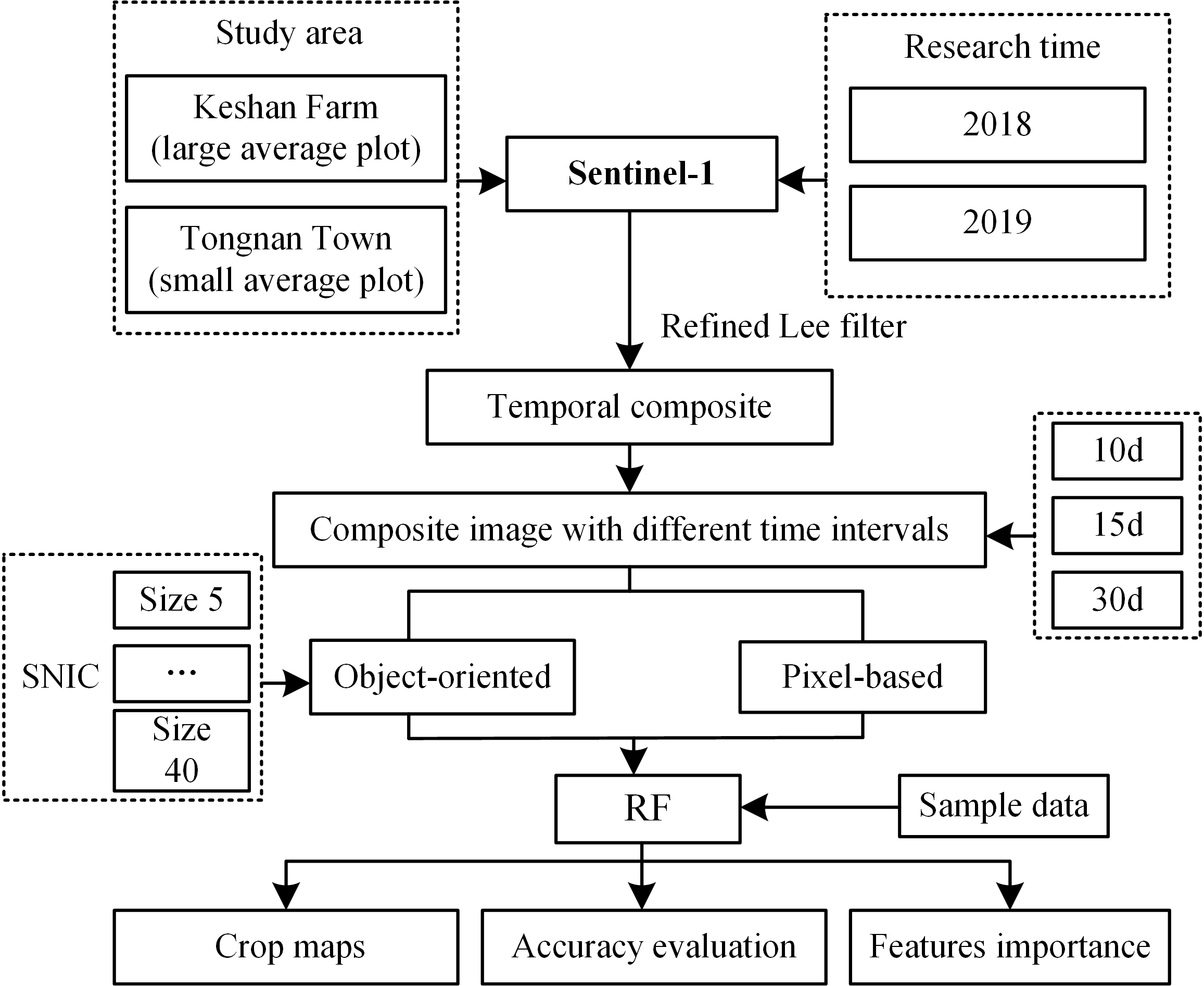
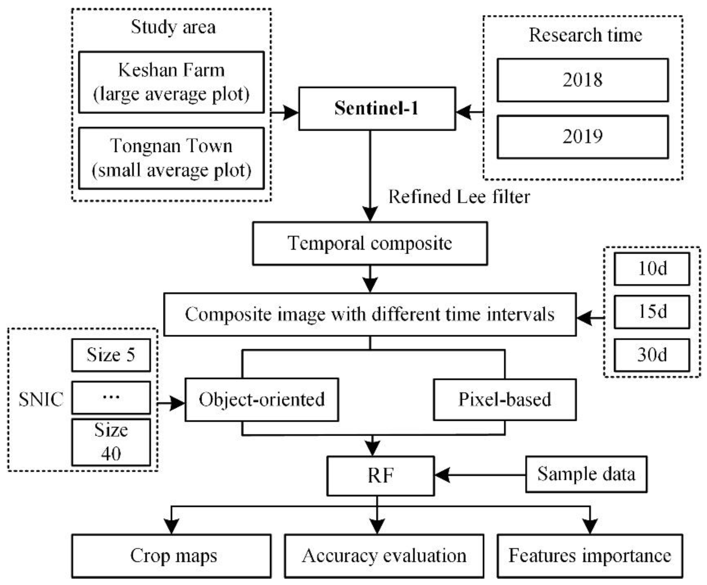
2. Materials and Methods

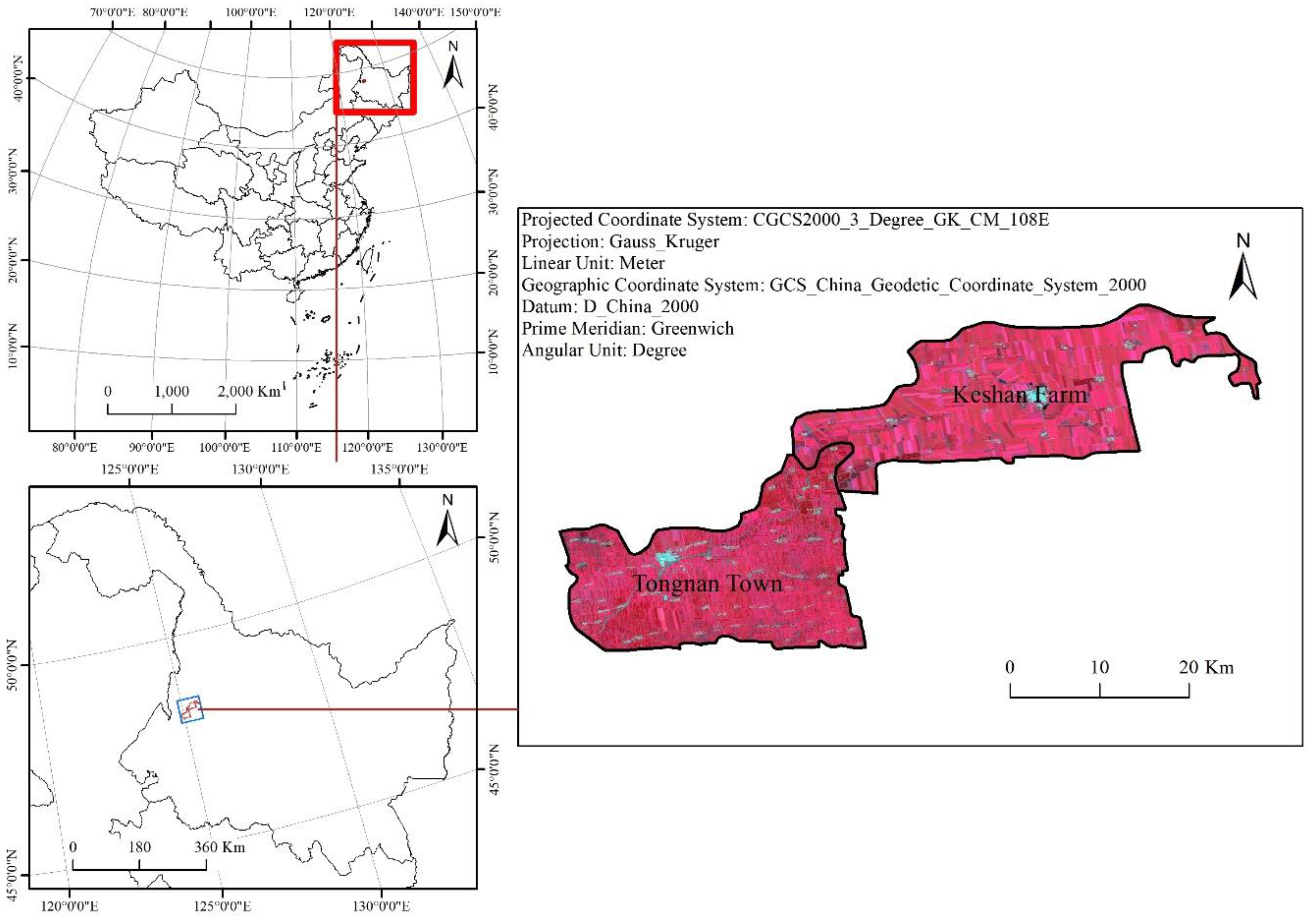
To study the potential of using object-oriented and time series Sentinel-1 in crop classification in GEE, two study areas with large differences in plot size were selected in this study. First, the Sentinel-1 images with different time intervals were obtained by GEE processing, the images were segmented by the simple noniterative clustering (SNIC) image segmentation method and then the processed images were classified using a random forest classifier. Finally, the classification accuracies of different scenarios were compared to evaluate the effectiveness and applicability of the methods. The flowchart of this study is shown in Figure 1.

2.1. Study Area

To verify the applicability of the method, two study areas with different agricultural production scales were selected in this study: Keshan farm (125°07′40″, 125°37′30″E, 48°11′15″, 48°24′07″N) and Tongnan town (124°54′15″, 125°12′44″E, 48°2′40″, 48°15′13″N) in central Heilongjiang Province, China, the areas are 3.35 km² and 3.15 km² respectively. As shown in Figure 2, the two study areas are adjacent to each other. Keshan farm is a state-owned farm. In Tongnan town, small-scale farmers are used as the mode of agricultural production and management. Due to the different agricultural production scales and management modes, the average plot sizes in the two areas are quite different. Corn, soybean and rice account for more than 95% of the planting area in Heilongjiang Province [37]. The two study areas are mainly planted with corn, soybean and rice, which are representative for Heilongjiang Province.

Keshan farm and Tongnan town are located in the northeastern Songnen Plain, with hilly terrain and fertile soil suitable for crop growth. Both study areas belong to the warm and cool type climate zone, which is characterized by a dry and windy spring, a high-temperature and rainy summer, rapid cooling in autumn, an early frost and a long winter that has snow and is cold and dry. The annual precipitation is approximately 502.5 mm and the precipitation in 6–8 months accounts for 68.3% of the annual amount. The frost-free period is only 120 days and only one growing season is guaranteed. The main crops are corn, soybean and rice and are generally sown in spring (April to May) and harvested in autumn (September to October). In fact, the crops have not grown at the end of April and the crops have basically been harvested at the beginning of October. Then we will take May to September as the study period. See

Table 1. Main crop calendar of the study area.

	Jan	Feb	Mar	Apr	May	Jun	Jul	Aug	Sep	Oct	Nov	Dec
corn					S	G	G	G	H	H
rice					S	G	G	G	H	H
soybeans					S	G	G	G	H

Note: S—Sowing; G—Growing; H—Harvesting.

for details and more information on the major crop calendar in the study area.

2.2. Data Selection and Preprocessing

2.2.1. Sentinel-1 SAR Image and Preprocessing

In this study, the Sentinel-1 SAR GRD dataset stored in the GEE cloud platform was used and it included all images covering the study area in 2018 and 2019 (May to September), including 27 images in 2018 and 22 images in 2019, it is very close to the temporal resolution of sentinel-1 which is usually reported as 6d [38]. The Sentinel-1 SAR GRD dataset was collected using the interference wide-band (IW) mapping mode, with a spatial resolution of 10 m, a width of 250 km and an average incidence angle of 30–45°. Each Sentinel-1 image stored by the GEE platform, which had been preprocessed using the European Space Agency’s (ESA) Sentinel-1 Toolbox including orbit restitution, thermal noise removal, terrain correction and radiometric calibration [39,40,41].

In addition, all Sentinel-1 images to be used were filtered with refined Lee filter on the GEE platform to reduce speckle. The function of each speckle filter should be adjusted according to local image variations to smooth the values and thereby reduce speckle and lines and edges are enhanced to maintain the sharpness of the imagery. This refined Lee filter was chosen because it could better retain polarization information under the influence of speckle elimination [42,43].

To evaluate the impact of Sentinel-1 images with different time intervals on classification accuracy, the median value of observations in each temporal interval was obtained and image time series were built. We use day of year (DOY) to represent time series.

2.2.2. Reference Data

The sample plots of this study came from the land by insurance companies and the crop type was confirmed on the spot. In 2018, there were 483 sample plots in Keshan farm, including 200 corn plots, 268 soybean plots and 15 rice plots; in 2019, there were 486 sample plots, including 272 corn plots, 203 soybean plots and 11 rice plots. There were 511 sample plots in Tongnan town in 2018, including 204 corn plots, 305 soybean plots and 2 rice plots; there were 542 sample plots in 2019, including 201 corn plots, 339 soybean plots and 2 rice plots. To avoid the time-out of GEE calculation, we used ArcGIS 10.3 to transform these sample plots into sample points. Each study area randomly selected 70% of the sample points as the training samples and 30% of the sample points as the verification samples. The plots in the study area are shown in

Table 2. Plot characteristics of Keshan farm and Tongnan town.

	Location	Number of Plots	Average Area (m2)	Average Circumference (m)	Average Area Circumference Ratio
2018	Keshan Farm	483	333,499.50	3126.49	101.77
2019	Keshan Farm	486	342,129.04	3137.81	103.94
2018	Tongnan Town	511	29,175.02	1256.92	21.15
2019	Tongnan Town	542	40,173.86	1313.92	26.85

.

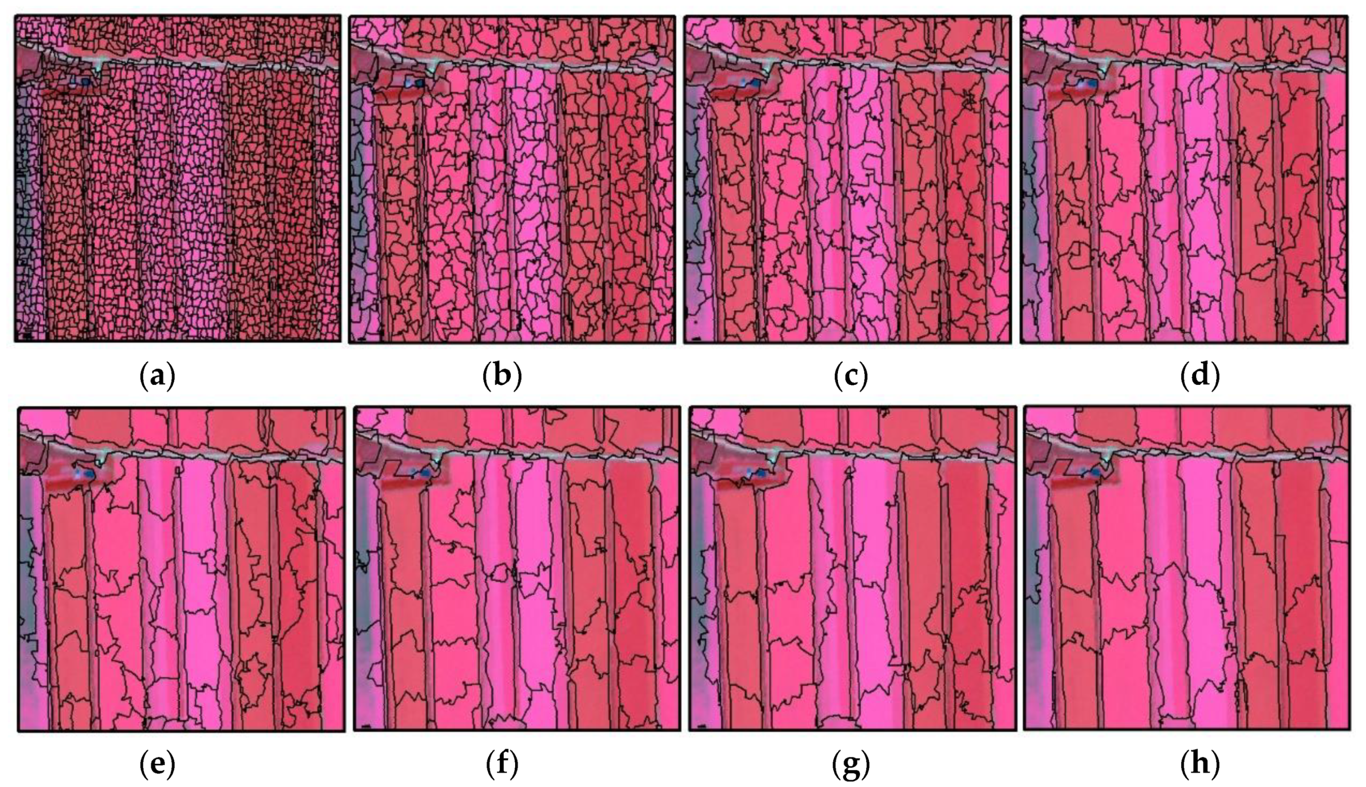
2.3. Image Segmentation

The traditional pixel-based classification method may produce “salt and pepper” noise, especially for Sentinel-1 radar data. The object-based algorithm reduces this problem by considering the neighborhood information of a given pixel to divide the image into specific areas or objects according to certain parameters. In this study, the SNIC image segmentation algorithm in GEE was used for image segmentation [44]. Firstly, the centroid pixels on the regular grid in the image are initialized. Next, the distance of pixels in the five-dimensional space of color and spatial coordinates is used to determine the dependency of each pixel relative to the centroid. At last, the distance integrates the normalized spatial and color distances to produce efficient, compact and nearly uniform polygons [45]. The main parameters of the SNIC algorithm are “image”, “size”, “compactness”, “connectivity”, “neighborhood size” and “seeds.” Among them, “image” is the image participating in segmentation. In this study, Sentinel-1 time series images with different time intervals composites in 2018 and 2019 (May to September) in two study areas were segmented. “Size” refers to the spacing of super-pixel seed positions based on pixels, that is, segmentation size. According to the situation of the study area, the “size” was set as “5”, “10”, “15”, “20”, “25”, “30”, “35” and “40” and the impact of different segmentation sizes on classification accuracy was evaluated. “Compactness” is compactness and the larger the value is, the closer the segmentation results are to the square; however, because the parcels in the study area were mostly rectangular, this study set the “compactness” value to 0. “Connectivity” stands for connectivity, which was set to 8 in this study. “Seeds” does not need to be set in this article, because the plot in this study area is closer to the rectangle. In the classification experiment using Sentinel-1 images, according to the experimental setting, each time interval has one original data control group and eight different size segmentation groups, for a total of three time interval composites, meaning each study area had 27 experimental groups every year.

2.4. Random Forest

Random forest is an improved self-classification and decision tree (CART), which is the most popular machine learning algorithm used for remote sensing classification [46,47]. The bootstrap sampling technique is employed to randomly extract a certain number of samples from the original dataset to generate a new training dataset. Each tree in the forest grows to the maximum extent without any trimming. The random sampling process avoids the occurrence of over-fitting. Random forest has many advantages over other algorithms [48,49]. First, random forest has been proven to be superior to other algorithms in classification accuracy. Second, random forest can process data with high dimensions without feature selection. The random forest algorithm uses bootstrap sampling technology to randomly select a certain number of samples from the original data set to generate a new training data set. Every tree in the forest can grow to its maximum without pruning. Random sampling process avoids overfitting [50].

It is very easy to use the random forest algorithm in the GEE cloud platform. In this study, we set the nTree value to 300, which can ensure accuracy and avoid overfitting [51]. Mtry was set to the default value, which was the square root of the input feature data.

Random forest classifiers usually use two methods to measure the importance of features relative to classification. MDA and MDG are, respectively, the average value of decreasing accuracy of a feature and the value of the decreasing Gini coefficient in random forest when other conditions are unchanged [46,47]. The higher the MDG value is, the more important this feature is. The higher the MDA value is, the more important the feature is. In this study, we used the MDA to evaluate the importance of different features. The principle of MDA value is to disrupt the eigenvalue order of each feature and to measure the influence of the order change on the accuracy of the model. This ingenious method uses out of pocket data to calculate importance. OOB (out-of-bag) data is a part of the training set but it is not used to train this special tree. OOB data is used to calculate the basic error and then the order of each feature is randomly scrambled. We used the R language package randomForest 4.6 to obtain the MDA value of the different features.

2.5. Accuracy Verification

In this study, the total accuracy (OA), kappa coefficient, producer accuracy (PA) and user accuracy (UA) were selected to evaluate the accuracy of crop classification [52]. The formulas are listed below:

$$\mathrm{OA} (\%)=\frac{{{\displaystyle \sum }}_{i=1}^n{p}_{ii}}{N}\times 100$$

(1)

$$\mathrm{Kappa}=\frac{N{{\displaystyle \sum }}_{i=1}^n{P}_{ii}-{{\displaystyle \sum }}_{i=1}^n\left(P_{i+}\times P_{+i}\right)}{N^2-{{\displaystyle \sum }}_{i=1}^n\left(P_{i+}\times P_{+i}\right)}$$

(2)

$$\mathrm{UA} (\%)=\frac{P_{ii}}{P_{i+}}\times 100$$

(3)

$$\mathrm{PA} (\%)=\frac{P_{ii}}{P_{+i}}\times 100$$

(4)

Here, n is the total number of columns of the confusion matrix; that is, the total number of categories, $P_{ii}$ is the number of correct classifications of the upper crop-type sample in the i-th row and i-th column of the confusion matrix, $P_{i+}$ and $P_{+i}$ are the total number of crop-type samples in row i and column i and N is the total number of samples used for verification.

3. Results

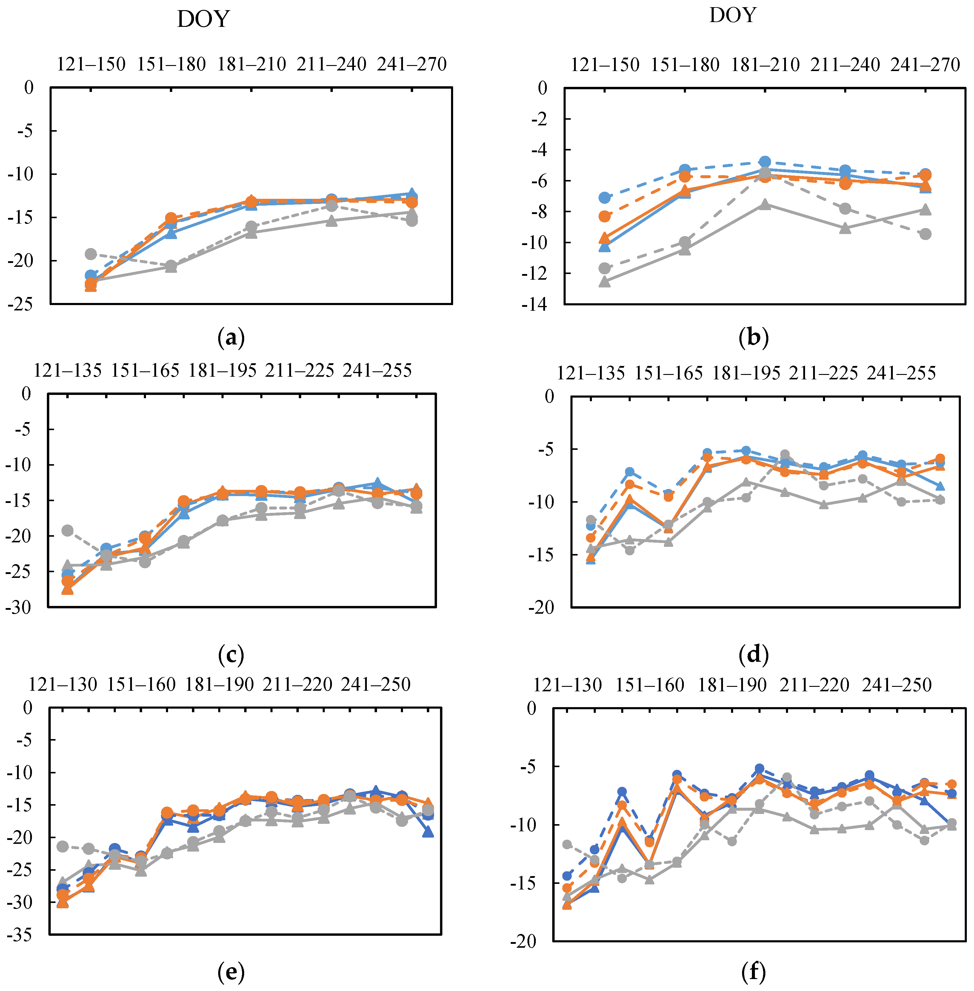
3.1. Sentinel-1 Time Series

Figure 3 shows the multitemporal images curves of the average backscatter coefficients of all samples of each crop type in the two study areas in 2018. In Figure 3, the X axis is the time series of images at different time intervals composites and the Y axis is the value of the backscattering coefficient. In the multitemporal images with a time interval of 30 d in the two study areas, the VH and VV bands in June, July, August and September easily identify rice, while the difference between corn and soybean is small. In the multitemporal images with a time interval of 15 d in the two study areas, the difference between rice and other crops is obvious in most periods. The difference between corn and soybean is more obvious in the first half of September and the second half of September in the VH band and more obvious in the second half of September in the VV band. In the multitemporal images with a time interval of 10 d in the two study areas, the difference between rice and other crops is still obvious. The difference between corn and soybean can be distinguished by the VH band in early September and late September or by the VV band in early August and late September.

3.2. Overall Accuracy Assessment

Table 3. The overall accuracies obtained using different classification schemes in different study areas.

Year	Study Area	Interval		Size
			Pixel	5	10	15	20	25	30	35	40
2018	Keshan Farm	10 d	84.99	88.10	93.20	93.77	94.62	92.92	95.47	94.33	94.05
		15 d	79.89	87.25	91.22	93.77	93.20	94.05	94.05	93.48	91.78
		30 d	69.41	77.62	84.42	87.82	88.10	88.95	86.69	88.10	86.69
	Tongnan Town	10 d	72.04	76.08	76.88	76.88	74.19	72.04	73.12	75.54	69.62
		15 d	75.00	74.19	73.39	74.46	75.81	73.12	72.04	73.92	69.89
		30 d	71.51	75.81	71.51	72.31	71.77	67.20	68.01	64.78	68.55
2019	Keshan Farm	10 d	80.66	90.33	92.75	94.86	93.96	94.86	94.26	94.56	93.66
		15 d	79.15	85.20	90.03	92.45	90.94	94.26	93.05	93.05	94.26
		30 d	76.44	83.08	85.20	88.82	91.54	91.24	92.45	92.15	92.75
	Tongnan Town	10 d	79.58	80.90	78.51	77.45	73.47	75.60	72.94	72.68	72.15
		15 d	78.51	78.78	76.13	76.13	75.86	79.58	75.86	72.41	72.94
		30 d	68.70	74.80	70.56	70.56	71.88	71.35	70.29	72.68	70.29

and

Table 4. The kappa coefficients obtained using different classification schemes in different study areas.

Year		Interval		Size
			Pixel	5	10	15	20	25	30	35	40
2018	Keshan Farm	10 d	0.70	0.77	0.87	0.88	0.90	0.87	0.91	0.89	0.89
		15 d	0.60	0.75	0.83	0.88	0.87	0.89	0.89	0.88	0.84
		30 d	0.40	0.56	0.70	0.76	0.77	0.79	0.74	0.77	0.75
	Tongnan Town	10 d	0.44	0.52	0.54	0.54	0.49	0.45	0.47	0.52	0.40
		15 d	0.50	0.49	0.47	0.50	0.52	0.47	0.44	0.48	0.41
		30 d	0.43	0.52	0.44	0.45	0.44	0.35	0.37	0.30	0.38
2019	Keshan Farm	10 d	0.61	0.81	0.86	0.90	0.88	0.90	0.89	0.89	0.88
		15 d	0.57	0.70	0.80	0.85	0.82	0.89	0.86	0.86	0.89
		30 d	0.54	0.67	0.71	0.78	0.83	0.83	0.85	0.85	0.86
	Tongnan Town	10 d	0.58	0.61	0.56	0.54	0.45	0.51	0.44	0.44	0.42
		15 d	0.57	0.57	0.51	0.52	0.51	0.58	0.51	0.45	0.45
		30 d	0.33	0.46	0.39	0.40	0.42	0.42	0.39	0.44	0.38

list the OAs and kappa coefficients of the different classification schemes for Sentinel-1 time series images using different time intervals composite for Keshan farm and Tongnan town in 2018 and 2019. At Keshan farm in 2018, Sentinel-1 with a time interval of 10 d obtained the highest crop classification accuracy when the image segmentation size was 30 (Figure 4). At Keshan farm in 2019, Sentinel-1 with a time interval of 10 d obtained the highest crop classification accuracy when the image segmentation size was 25 (Figure 5). In Tongnan town in 2018, Sentinel-1 with a time interval of 10 d obtained the highest crop classification accuracy when the image segmentation size was 15 (Figure 6). In Tongnan town in 2019, Sentinel-1 with a time interval of 10 d obtained the highest crop classification accuracy when the image segmentation size was 5 (Figure 7).

In Keshan farm, where the average plot was large, the shorter time interval of Sentinel-1 composite was, the higher the accuracy of crop classification was; compared with the pixel-based classification method, the accuracy of using the object-oriented classification method was greatly improved. In Tongnan town, where the average plot was small, in most cases, the shorter time interval of Sentinel-1 composite was, the higher the accuracy of crop classification was; an exception was the pixel-based classification in 2018. when the time interval decreased from 15 d to 10 d, the accuracy of crop classification decreased; compared with the pixel-based classification accuracy, using the object-oriented classification method in Tongnan town did not result in an obvious improvement.

3.3. User Accuracy and Producer Accuracy

Figure 8 and Figure 9 show the user accuracy (UA) and producer accuracy (PA) for images with different time intervals using pixel-based and object-oriented classification (optimal size) in Keshan farm and Tongnan town. For Keshan farm in 2018, Sentinel-1 with a time interval of 10 d combined with object-oriented classification achieved the highest UA and PA for corn and rice, Sentinel-1 with a time interval of 15 d combined with object-oriented classification achieved the highest PA for soybean (Figure 8). Compared with pixel-based classification, object-oriented classification always had a higher UA. In 2019, the PA and UA of different crops showed similar performance as that in 2018 (Figure 8) and the time interval between 10 d and 15 d was not much different between UA and PA.

In Tongnan town, there was no significant difference in the PA and UA between corn and soybean based on pixel classification compared with object-oriented classification and the PA and UA of corn and soybean changed irregularly with different time intervals (Figure 9).

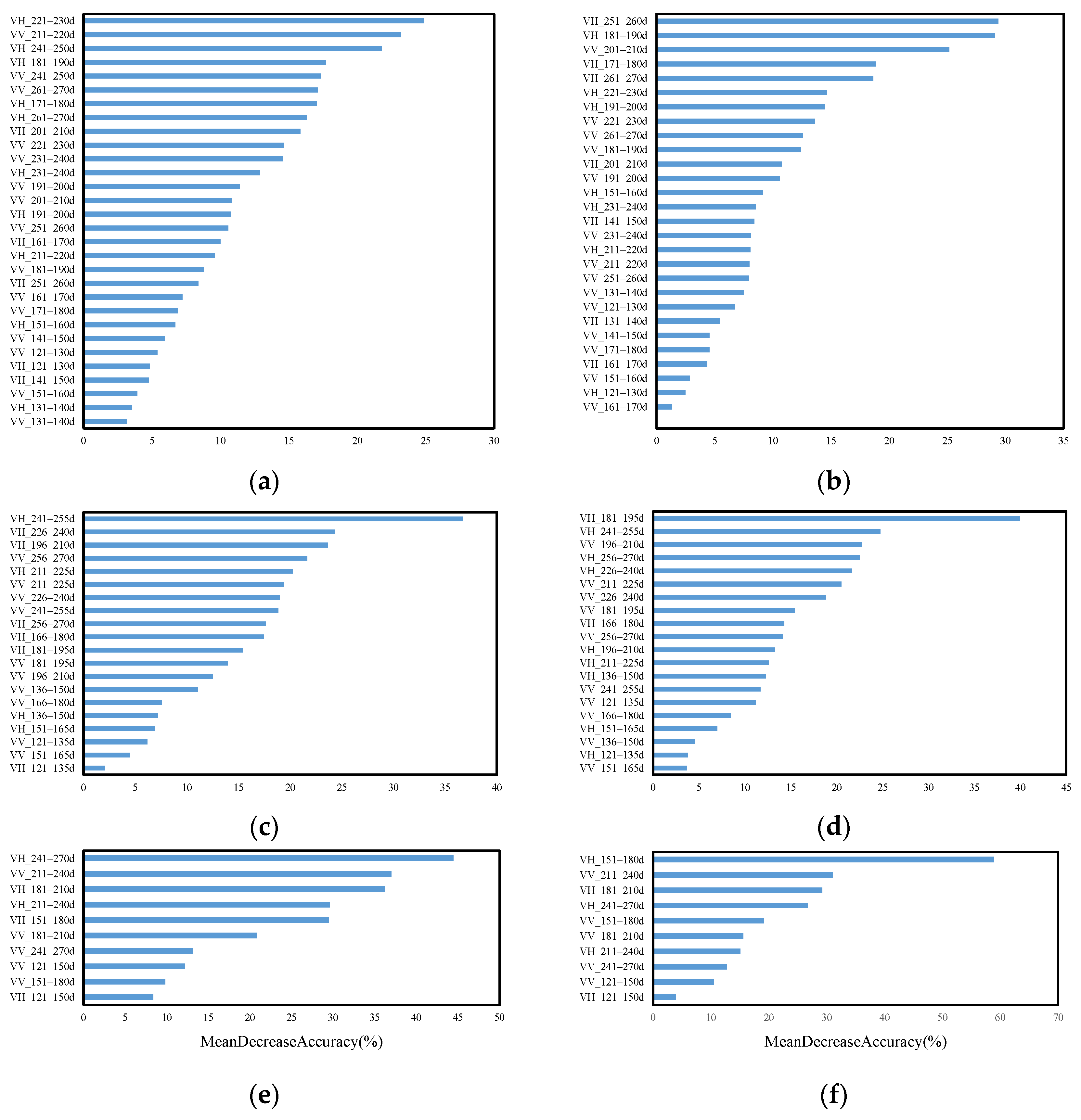
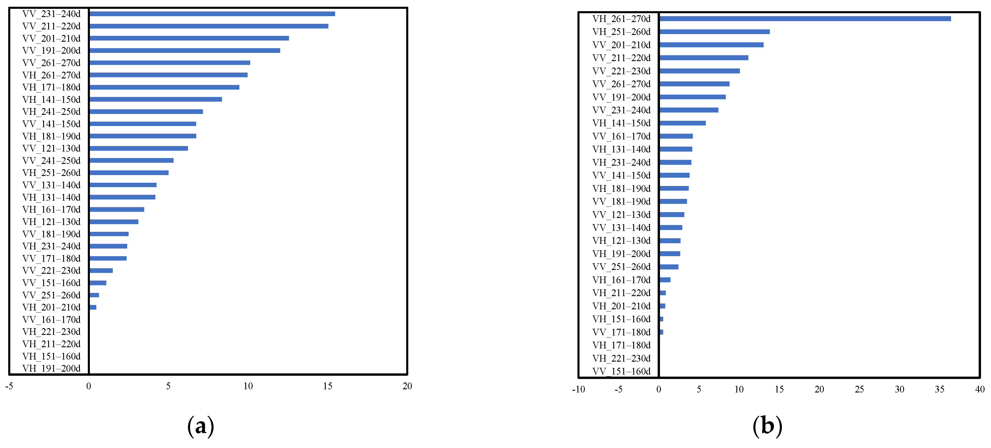
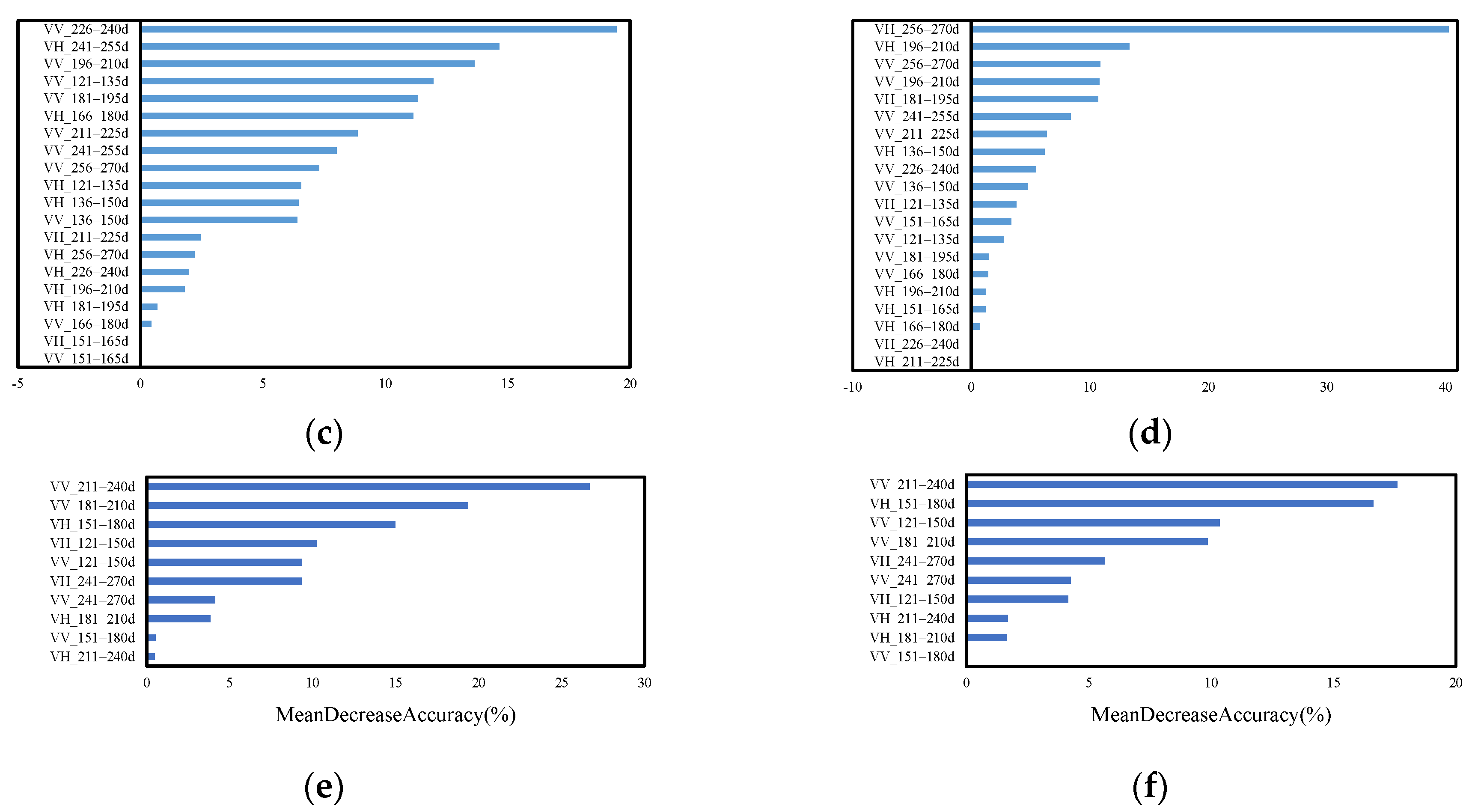
3.4. Features Importance Assessment

In addition, this study evaluated the importance features of Sentinel-1 images with different time intervals in Keshan farm and Tongnan town (object-oriented with optimal segmentation size). When using Sentinel-1 images with 10-d time interval for crop classification in Keshan farm and Tongnan town, the VH band in 2019 was more important than that in 2018, which may be due to the reduced importance of the water-sensitive VV band in crop classification due to the flood in 2019. This situation was not obvious when using Sentinel-1 images with a time interval of 15 d or 30 d, mainly because the effect of flood was eliminated by using the median value of a longer time interval (Figure 10 and Figure 11).

The features with higher importance in Sentinel-1 images with different time intervals were mainly distributed in July, August and September, which was mainly due to the large differences in the structure of different crops in July, August and September. When corn enters the heading stage in July, the dry matter on the ground increases rapidly and the differences between corn and soybean increase. The features with higher importance in different years also have differences, which may be caused by the differences in crop phenology in different years.

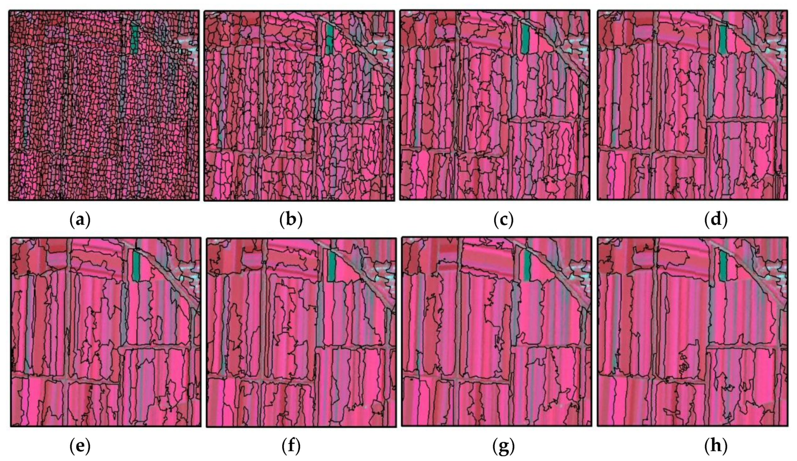
3.5. Determination of the Optimal Segmentation Size

The traditional method of determining the optimal segment size in object-oriented classification usually involves conducting repeated experiments. From Table 2, we can obtain the average area and average perimeter of sample plots in Keshan farm and Tongnan town in 2018 and 2019. We assume that the plots in the study area are evenly distributed rectangles and the average side length of the plots can be calculated from the perimeter and area. The long-side length and short-side length are shown in

Table 5. The relationship between the optimal segment size and the side length of the plot.

	Number	Average Long Side	Average Short Side	Average Optimal Size	Average Short Side/Image Resolution
2018 ks	493	1308.03	254.96	26.67	25.50
2019 ks	486	1306.04	261.95	30	26.20
2018 tn	511	577.48	50.52	13.33	5.05
2019 tn	542	587.64	68.36	11.67	6.84

. We can obtain the following relationship: the best segmentation size ≈ average short side/image resolution. This relationship is better applied to the large plot of Keshan farm but is slightly less applicable to the small plot of Tongnan town.

4. Discussion

4.1. Advantages of Using Time Series Sentinel-1 Images Combined with Object-Oriented Classification Methods

In the past, research on crop classification using SAR data usually focused on obtaining more useful information from different polarizations to improve the accuracy of crop classification [53,54,55]. Therefore, RADARSAT-2 data are usually used as the data source because compared with single polarization and dual-polarization radar data, multi-polarization RADARSAT-2 data (HH, HV, VV, VH) have obvious advantages in crop classification [56].

Dense time series images can provide more detailed phenology information, which has been proven to improve the accuracy of crop classification [16] but RADARSAT-2 has a revisit period of 24 d, making it difficult to obtain dense time series data. The theoretical revisit period of Sentinel-1 data used in this study is 6 d and its temporal resolution can effectively meet the requirements of time series-based classification methods. The research in this study proves that using Sentinel-1 composite images with a shorter time interval can improve the accuracy of crop classification in most cases.

Many studies have proven that object-oriented classification is superior to pixel-based classification [57,58]. Previous studies have often used ready-made plot data directly so that crops within the parcel can be directly identified [26] but most developing countries do not have complete plot databases and there is no guarantee of the uniqueness of the crops grown on each plot. In this study, the image segmentation algorithm was used to segment the multitemporal images into “blocks” and then the pixels in the “blocks” were regarded as being the same class, thereby reducing the impact of speckle noise in SAR images on the classification accuracy. This study shows that the accuracy of crop classification can be improved to a very high level (OA > 90%) by using the method of object-oriented classification and time series Sentinel-1 in the case of a large plot size.

4.2. Advantages of Using GEE

The GEE cloud platform effectively promoted this research. GEE has been proved to be very suitable for high-speed data analysis with large spatial processing functions [34,35]. In this study, we used GEE to select Sentinel-1 images, used refined Lee filter to reduce speckles, composited the processed Sentinel-1 images according to different time intervals, used the SNIC algorithm for image segmentation and finally used random forest for crop classification. In this study, except for the band importance evaluation that was processed in R Studio, all other processes were performed in the GEE cloud platform. If these works are carried out offline, it may take several days to dozens of days. In the GEE cloud platform, we focus on experimental design and code writing, which greatly improved the efficiency of crop classification. In addition, GEE integrates many other machine learning algorithms and image segmentation algorithms, which provides the possibility of future algorithm improvements.

4.3. The Relationship between Image Resolution and Optimal Segmentation Size

Through the analysis of sample characteristics in Table 2, we see that the average plot area of Keshan farm is approximately 10 times that of Tongnan town and the average plot area perimeter ratio of Keshan farm is approximately 5 times that of Tongnan town, which shows that the plot of study area a is closer to the square, which is beneficial for image segmentation.

It can be seen from Figure 12 that when the segmentation size of Keshan farm is 25 or 30, the segmentation result is closest to the boundary of the plot. At this time, the accuracy of crop classification is the highest. If the segmentation size is too large, two adjacent plots are mixed together; in contrast, if the segmentation size is too small, the speckle noise cannot be removed well. Figure 13 shows that when the segmentation size of Tongnan town is 5, the segmentation result has mixed two adjacent plots together and the accuracy of object-oriented classification is not much better than that of pixel-based classification. Of course, this method of judging the optimal segmentation size is applicable only to areas with little difference in plot area.

4.4. Uncertainty of the Method

The method proposed in this study has been proven to achieve good results in Keshan farm with a large plot area for two consecutive years. The highest OA of object-oriented classification was approximately 95%, which was 10% higher than that of pixel-based classification. However, in Tongnan town, which has a small plot area, the highest OA of the object-oriented classification method was only approximately 2% higher than that of the pixel-based classification method (Table 3). This difference is mainly because the resolution of the Sentinel-1 image is 10 m and the plot in Tongnan town is too small. If the segmentation size is small, the speckle noise of Sentinel-1 cannot be eliminated. If the segmentation size is large, the “block” after segmentation may contain adjacent plots, resulting in classification errors. We believe that this result does not mean that the object-oriented classification method does not work in the small area of the plot but rather that the object-oriented method needs to match the SAR image of the appropriate spatial resolution. When the resolution of the SAR image is too low to the short-side length of the plot, ideal accuracy cannot be obtained. In addition, since there are only three crops in this study, the effect of the model in the more complex area of crop types needs further study. Most of the previous studies highlight the advantages of object-oriented classification method [26,59,60]. Our research shows that object-oriented classification method has almost no advantages over pixel-based method in some areas, which provides a reference for future research.

4.5. Future Research Directions

Crop classification maps are the basis of precise agricultural management [61]. It is of great significance for regional food security and sustainable development to produce annual crop distribution maps regularly [62]. Optical images have shown good performance in crop classification but in areas with hot and rainy seasons, there are many clouds covering the critical period of crop growth every year and cloud presence seriously affects the observation of optical images. At this time, it is very important to evaluate the potential use of SAR data for crop classification.

In this study, the method of using the object-oriented method combined with the multitemporal Sentinel-1 images method in GEE had an obvious effect in large plot areas but the effect in small plot areas was not obvious. The method to solve the poor effect of small plot area classification is to use SAR images with a higher spatial resolution combined with object-oriented methods. In addition, in this study, it was found that with the decrease in time interval composite from 15 d to 10 d, the accuracy of crop classification was not significantly improved; thus, we speculated that the object-oriented method combined with SAR images with higher spatial resolutions can achieve ideal accuracy without too high of a temporal resolution. In the next step, we will test whether the higher spatial resolution SAR data gaofen-3 (the highest spatial resolution is 1 m) combined with object-oriented method can significantly improve the accuracy of crop classification in small plot area. In addition, some studies have shown that band ratio or sentinel-1 radar vegetation index can better monitor agricultural land use [63] and other studies have proved that deep learning algorithm combined with SAR data can obtain higher crop classification accuracy [64], these are the directions that need further research.

5. Conclusions

The results emphasize the influence of the time interval and segmentation size of the composite image on the accuracy of crop classification when using sentinel-1 composite image combined with object-oriented classification. The composite image with shorter time interval can provide more information for crop classification, so as to improve the accuracy of crop classification. It was found that using the object-oriented classification method combined with Sentinel-1 data in GEE greatly improved the accuracy of crop classification in large plot area. The object-oriented classification method obviously improves the “salt and pepper phenomenon”, which is common in SAR data classification results, because the method divides the image into “block” crop processing units to suppress noise. This approach also leads to the close relationship between object-oriented crop classification accuracy and the image segmentation effect. The closer the image segmentation result is to the real land distribution, the higher the accuracy of crop classification is. With the more popular use of GEE, more advanced image segmentation and more advanced machine learning combined with GEE will obtain more accurate crop classification results. In addition, this study evaluated the band importance of Sentinel-1 in two consecutive years crop classification. The results showed that the features with higher importance were mainly distributed in July, August and September and there were differences in the features with higher importance in different years. Our study also found that the optimal segmentation size of object-oriented classification was closely related to the short-side length and image resolution.

References

1. Carvalho, F.P. Agriculture, pesticides, food security and food safety. Environ. Sci. Policy 2006, 9, 685–692. [Google Scholar] [CrossRef]
2. McMichael, P. The power of food. Agric. Hum. Values 2000, 17, 21–33. [Google Scholar] [CrossRef]
3. Schmidhuber, J.; Tubiello, F.N. Global food security under climate change. Proc. Natl. Acad. Sci. USA 2007, 104, 19703–19708. [Google Scholar] [CrossRef] [Green Version]
4. Garnett, T.; Appleby, M.C.; Balmford, A.; Bateman, I.J.; Benton, T.G.; Bloomer, P.; Burlingame, B.; Dawkins, M.; Dolan, L.; Fraser, D. Sustainable intensification in agriculture: Premises and policies. Science 2013, 341, 33–34. [Google Scholar] [CrossRef] [PubMed]
5. Godfray, H.C.J.; Crute, I.R.; Haddad, L.; Lawrence, D.; Muir, J.F.; Nisbett, N.; Pretty, J.; Robinson, S.; Toulmin, C.; Whiteley, R. The future of the global food system. Philos. Trans. R Soc. Lond. B Biol. Sci. 2010, 365, 2769–2777. [Google Scholar] [CrossRef] [PubMed] [Green Version]
6. Opara, L.U. Traceability in agriculture and food supply chain: A review of basic concepts, technological implications, and future prospects. J. Food Agric. Environ. 2003, 1, 101–106. [Google Scholar]
7. Davis, K.F.; Rulli, M.C.; Seveso, A.; D’Odorico, P. Increased food production and reduced water use through optimized crop distribution. Nat. Geosci. 2017, 10, 919. [Google Scholar] [CrossRef]
8. Rockström, J.; Williams, J.; Daily, G.; Noble, A.; Matthews, N.; Gordon, L.; Wetterstrand, H.; DeClerck, F.; Shah, M.; Steduto, P. Sustainable intensification of agriculture for human prosperity and global sustainability. AMBIO 2017, 46, 4–17. [Google Scholar] [CrossRef] [Green Version]
9. Pervez, M.S.; Brown, J.F. Mapping irrigated lands at 250-m scale by merging MODIS data and national agricultural statistics. Remote Sens. 2010, 2, 2388–2412. [Google Scholar] [CrossRef] [Green Version]
10. Gumma, M.K.; Thenkabail, P.S.; Maunahan, A.; Islam, S.; Nelson, A. Mapping seasonal rice cropland extent and area in the high cropping intensity environment of Bangladesh using MODIS 500 m data for the year 2010. ISPRS J. Photogramm. Remote Sens. 2014, 91, 98–113. [Google Scholar] [CrossRef]
11. Joshi, N.; Baumann, M.; Ehammer, A.; Fensholt, R.; Grogan, K.; Hostert, P.; Jepsen, M.R.; Kuemmerle, T.; Meyfroidt, P.; Mitchard, E.T. A review of the application of optical and radar remote sensing data fusion to land use mapping and monitoring. Remote Sens. 2016, 8, 70. [Google Scholar] [CrossRef] [Green Version]
12. Huang, Y.; Chen, Z.-x.; Tao, Y.; Huang, X.-z.; Gu, X.-f. Agricultural remote sensing big data: Management and applications. J. Integr. Agric. 2018, 17, 1915–1931. [Google Scholar] [CrossRef]
13. Kussul, N.; Lemoine, G.; Gallego, F.J.; Skakun, S.V.; Lavreniuk, M.; Shelestov, A.Y. Parcel-based crop classification in ukraine using landsat-8 data and sentinel-1A data. IEEE J. Sel. Top. Appl. Earth Obs. Remote Sens. 2016, 9, 2500–2508. [Google Scholar] [CrossRef]
14. Kussul, N.; Lavreniuk, M.; Skakun, S.; Shelestov, A. Deep learning classification of land cover and crop types using remote sensing data. IEEE Geosci. Remote Sens. Lett. 2017, 14, 778–782. [Google Scholar] [CrossRef]
15. Belgiu, M.; Csillik, O. Sentinel-2 cropland mapping using pixel-based and object-based time-weighted dynamic time warping analysis. Remote Sens. Environ. 2018, 204, 509–523. [Google Scholar] [CrossRef]
16. Griffiths, P.; Nendel, C.; Hostert, P. Intra-annual reflectance composites from Sentinel-2 and Landsat for national-scale crop and land cover mapping. Remote Sens. Environ. 2019, 220, 135–151. [Google Scholar] [CrossRef]
17. Foga, S.; Scaramuzza, P.L.; Guo, S.; Zhu, Z.; Dilley Jr, R.D.; Beckmann, T.; Schmidt, G.L.; Dwyer, J.L.; Hughes, M.J.; Laue, B. Cloud detection algorithm comparison and validation for operational Landsat data products. Remote Sens. Environ. 2017, 194, 379–390. [Google Scholar] [CrossRef] [Green Version]
18. Zhu, Z.; Wang, S.; Woodcock, C.E. Improvement and expansion of the Fmask algorithm: Cloud, cloud shadow, and snow detection for Landsats 4–7, 8, and Sentinel 2 images. Remote Sens. Environ. 2015, 159, 269–277. [Google Scholar] [CrossRef]
19. Blaes, X.; Vanhalle, L.; Defourny, P. Efficiency of crop identification based on optical and SAR image time series. Remote Sens. Environ. 2005, 96, 352–365. [Google Scholar] [CrossRef]
20. Ndikumana, E.; Ho Tong Minh, D.; Baghdadi, N.; Courault, D.; Hossard, L. Deep recurrent neural network for agricultural classification using multitemporal SAR Sentinel-1 for Camargue, France. Remote Sens. 2018, 10, 1217. [Google Scholar] [CrossRef] [Green Version]
21. Xu, L.; Zhang, H.; Wang, C.; Zhang, B.; Liu, M. Crop Classification Based on Temporal Information Using Sentinel-1 SAR Time-Series Data. Remote Sens. 2019, 11, 53. [Google Scholar] [CrossRef] [Green Version]
22. Fu, W.; Ma, J.; Chen, P.; Chen, F. Remote Sensing Satellites for Digital Earth. In Manual of Digital Earth; Springer: Berlin, Germany, 2020; pp. 55–123. [Google Scholar]
23. Agrawal, S.; Raghavendra, S.; Kumar, S.; Pande, H. Geospatial Data for the Himalayan Region: Requirements, Availability, and Challenges. In Remote Sensing of Northwest Himalayan Ecosystems; Springer: Berlin, Germany, 2019; pp. 471–500. [Google Scholar]
24. Liu, C.-A.; Chen, Z.-X.; Yun, S.; Chen, J.-S.; Hasi, T.; Pan, H.-Z. Research advances of SAR remote sensing for agriculture applications: A review. J. Integr. Agric. 2019, 18, 506–525. [Google Scholar] [CrossRef] [Green Version]
25. Huang, X.; Wang, J.; Shang, J.; Liao, C.; Liu, J. Application of polarization signature to land cover scattering mechanism analysis and classification using multi-temporal C-band polarimetric RADARSAT-2 imagery. Remote Sens. Environ. 2017, 193, 11–28. [Google Scholar] [CrossRef]
26. Jiao, X.; Kovacs, J.M.; Shang, J.; McNairn, H.; Walters, D.; Ma, B.; Geng, X. Object-oriented crop mapping and monitoring using multi-temporal polarimetric RADARSAT-2 data. Isprs J. Photogramm. Remote Sens. 2014, 96, 38–46. [Google Scholar] [CrossRef]
27. Satalino, G.; Balenzano, A.; Mattia, F.; Davidson, M.W. C-band SAR data for mapping crops dominated by surface or volume scattering. IEEE Geosci. Remote Sens. Lett. 2013, 11, 384–388. [Google Scholar] [CrossRef]
28. Nagraj, G.M.; Karegowda, A.G. Crop Mapping using SAR Imagery: An Review. Int. J. Adv. Res. Comput. Sci. 2016, 7, 47–52. [Google Scholar]
29. Salehi, B.; Daneshfar, B.; Davidson, A.M. Accurate crop-type classification using multi-temporal optical and multi-polarization SAR data in an object-based image analysis framework. Int. J. Remote Sens. 2017, 38, 4130–4155. [Google Scholar] [CrossRef]
30. Tomppo, E.; Antropov, O.; Praks, J. Cropland Classification Using Sentinel-1 Time Series: Methodological Performance and Prediction Uncertainty Assessment. Remote Sens. 2019, 11, 2480. [Google Scholar] [CrossRef] [Green Version]
31. Gorelick, N.; Hancher, M.; Dixon, M.; Ilyushchenko, S.; Thau, D.; Moore, R. Google Earth Engine: Planetary-scale geospatial analysis for everyone. Remote Sens. Environ. 2017, 202, 18–27. [Google Scholar] [CrossRef]
32. Dong, J.; Xiao, X.; Menarguez, M.A.; Zhang, G.; Qin, Y.; Thau, D.; Biradar, C.; Moore III, B. Mapping paddy rice planting area in northeastern Asia with Landsat 8 images, phenology-based algorithm and Google Earth Engine. Remote Sens. Environ. 2016, 185, 142–154. [Google Scholar] [CrossRef] [Green Version]
33. Luo, C.; Liu, H.-j.; Fu, Q.; Guan, H.-x.; Ye, Q.; Zhang, X.-l.; Kong, F.-c. Mapping the fallowed area of paddy fields on Sanjiang Plain of Northeast China to assist water security assessments. J. Integr. Agric. 2020, 19, 1885–1896. [Google Scholar] [CrossRef]
34. Zurqani, H.A.; Post, C.J.; Mikhailova, E.A.; Cope, M.P.; Allen, J.S.; Lytle, B.A. Evaluating the integrity of forested riparian buffers over a large area using LiDAR data and Google Earth Engine. Sci. Rep. 2020, 10, 14096. [Google Scholar] [CrossRef] [PubMed]
35. Jia, M.; Wang, Z.; Mao, D.; Ren, C.; Wang, C.; Wang, Y. Rapid, robust, and automated mapping of tidal flats in China using time series Sentinel-2 images and Google Earth Engine. Remote Sens. Environ. 2021, 255, 112285. [Google Scholar] [CrossRef]
36. Malenovský, Z.; Rott, H.; Cihlar, J.; Schaepman, M.E.; García-Santos, G.; Fernandes, R.; Berger, M. Sentinels for science: Potential of Sentinel-1,-2, and-3 missions for scientific observations of ocean, cryosphere, and land. Remote Sens. Environ. 2012, 120, 91–101. [Google Scholar] [CrossRef]
37. You, N.; Dong, J. Examining earliest identifiable timing of crops using all available Sentinel 1/2 imagery and Google Earth Engine. ISPRS J. Photogramm. Remote Sens. 2020, 161, 109–123. [Google Scholar] [CrossRef]
38. Torres, R.; Snoeij, P.; Geudtner, D.; Bibby, D.; Davidson, M.; Attema, E.; Potin, P.; Rommen, B.; Floury, N.; Brown, M.; et al. GMES Sentinel-1 mission. Remote Sens. Environ. 2012, 120, 9–24. [Google Scholar] [CrossRef]
39. Sun, Z.; Luo, J.; Yang, J.; Yu, Q.; Zhang, L.; Xue, K.; Lu, L. Nation-Scale Mapping of Coastal Aquaculture Ponds with Sentinel-1 SAR Data Using Google Earth Engine. Remote Sens. 2020, 12, 3086. [Google Scholar] [CrossRef]
40. Hu, L.; Xu, N.; Liang, J.; Li, Z.; Chen, L.; Zhao, F. Advancing the Mapping of Mangrove Forests at National-Scale Using Sentinel-1 and Sentinel-2 Time-Series Data with Google Earth Engine: A Case Study in China. Remote Sens. 2020, 12, 3120. [Google Scholar] [CrossRef]
41. Gašparović, M.; Dobrinić, D. Comparative assessment of machine learning methods for urban vegetation mapping using multitemporal sentinel-1 imagery. Remote Sens. 2020, 12, 1952. [Google Scholar] [CrossRef]
42. Lee, J.-S.; Wen, J.-H.; Ainsworth, T.L.; Chen, K.-S.; Chen, A.J.J.I.T.o.G.; Sensing, R. Improved sigma filter for speckle filtering of SAR imagery. IEEE Trans. Geosci. Remote Sens. 2008, 47, 202–213. [Google Scholar]
43. Yommy, A.S.; Liu, R.; Wu, S. SAR image despeckling using refined Lee filter. In Proceedings of the 2015 7th International Conference on Intelligent Human-Machine Systems and Cybernetics, Hangzhou, China, 26–27 August 2015; pp. 260–265. [Google Scholar]
44. Achanta, R.; Susstrunk, S. Superpixels and polygons using simple non-iterative clustering. In Proceedings of the IEEE Conference on Computer Vision and Pattern Recognition, San Juan, PR, USA, 17–19 June 1997; pp. 4651–4660. [Google Scholar]
45. Mahdianpari, M.; Salehi, B.; Mohammadimanesh, F.; Homayouni, S.; Gill, E. The first wetland inventory map of newfoundland at a spatial resolution of 10 m using sentinel-1 and sentinel-2 data on the google earth engine cloud computing platform. Remote Sens. 2019, 11, 43. [Google Scholar] [CrossRef] [Green Version]
46. Liaw, A.; Wiener, M. Classification and regression by randomForest. R News 2002, 2, 18–22. [Google Scholar]
47. Pal, M. Random forest classifier for remote sensing classification. Int. J. Remote Sens. 2005, 26, 217–222. [Google Scholar] [CrossRef]
48. Belgiu, M.; Drăguţ, L. Random forest in remote sensing: A review of applications and future directions. ISPRS J. Photogramm. Remote Sens. 2016, 114, 24–31. [Google Scholar] [CrossRef]
49. Rodriguez-Galiano, V.F.; Ghimire, B.; Rogan, J.; Chica-Olmo, M.; Rigol-Sanchez, J.P. An assessment of the effectiveness of a random forest classifier for land-cover classification. ISPRS J. Photogramm. Remote Sens. 2012, 67, 93–104. [Google Scholar] [CrossRef]
50. Park, S.; Im, J.; Park, S.; Yoo, C.; Han, H.; Rhee, J. Classification and Mapping of Paddy Rice by Combining Landsat and SAR Time Series Data. Remote Sens. 2018, 10, 447. [Google Scholar] [CrossRef] [Green Version]
51. Tian, F.; Wu, B.; Zeng, H.; Zhang, X.; Xu, J. Efficient Identification of Corn Cultivation Area with Multitemporal Synthetic Aperture Radar and Optical Images in the Google Earth Engine Cloud Platform. Remote Sens. 2019, 11, 629. [Google Scholar] [CrossRef] [Green Version]
52. Story, M.; Congalton, R.G. Accuracy assessment: A user’s perspective. Photogramm. Eng. Remote Sens. 1986, 52, 397–399. [Google Scholar]
53. Lee, J.-S.; Grunes, M.R.; Pottier, E. Quantitative comparison of classification capability: Fully polarimetric versus dual and single-polarization SAR. IEEE Trans. Geosci. Remote Sens. 2001, 39, 2343–2351. [Google Scholar]
54. Skriver, H. Crop classification by multitemporal C-and L-band single-and dual-polarization and fully polarimetric SAR. IEEE Trans. Geosci. Remote Sens. 2011, 50, 2138–2149. [Google Scholar] [CrossRef]
55. Wu, F.; Wang, C.; Zhang, H.; Zhang, B.; Tang, Y. Rice crop monitoring in South China with RADARSAT-2 quad-polarization SAR data. IEEE Geosci. Remote Sens. Lett. 2010, 8, 196–200. [Google Scholar] [CrossRef]
56. Huang, X.; Liao, C.; Xing, M.; Ziniti, B.; Wang, J.; Shang, J.; Liu, J.; Dong, T.; Xie, Q.; Torbick, N. A multi-temporal binary-tree classification using polarimetric RADARSAT-2 imagery. Remote Sens. Environ. 2019, 235, 111478. [Google Scholar] [CrossRef]
57. Qi, Z.; Yeh, A.G.-O.; Li, X.; Lin, Z. A novel algorithm for land use and land cover classification using RADARSAT-2 polarimetric SAR data. Remote Sens. Environ. 2012, 118, 21–39. [Google Scholar] [CrossRef]
58. Skakun, S.; Kussul, N.; Shelestov, A.Y.; Lavreniuk, M.; Kussul, O. Efficiency assessment of multitemporal C-band Radarsat-2 intensity and Landsat-8 surface reflectance satellite imagery for crop classification in Ukraine. IEEE J. Sel. Top. Appl. Earth Obs. Remote Sens. 2015, 9, 3712–3719. [Google Scholar] [CrossRef]
59. Tassi, A.; Vizzari, M. Object-Oriented LULC Classification in Google Earth Engine Combining SNIC, GLCM, and Machine Learning Algorithms. Remote Sens. 2020, 12, 3776. [Google Scholar] [CrossRef]
60. Shen, G.; Yang, X.; Jin, Y.; Luo, S.; Xu, B.; Zhou, Q. Land Use Changes in the Zoige Plateau Based on the Object-Oriented Method and Their Effects on Landscape Patterns. Remote Sens. 2020, 12, 14. [Google Scholar] [CrossRef] [Green Version]
61. Hao, P.-Y.; Tang, H.-J.; Chen, Z.-X.; Meng, Q.-Y.; Kang, Y.-P. Early-season crop type mapping using 30-m reference time series. J. Integr. Agric. 2020, 19, 1897–1911. [Google Scholar] [CrossRef]
62. Hao, P.-Y.; Tang, H.-J.; Chen, Z.-X.; Le, Y.; Wu, M.-Q. High resolution crop intensity mapping using harmonized Landsat-8 and Sentinel-2 data. J. Integr. Agric. 2019, 18, 2883–2897. [Google Scholar] [CrossRef]
63. Holtgrave, A.-K.; Röder, N.; Ackermann, A.; Erasmi, S.; Kleinschmit, B. Comparing Sentinel-1 and -2 Data and Indices for Agricultural Land Use Monitoring. Remote Sens. 2020, 12, 2919. [Google Scholar] [CrossRef]
64. Cué La Rosa, L.E.; Queiroz Feitosa, R.; Nigri Happ, P.; Del’Arco Sanches, I.; Ostwald Pedro da Costa, G.A. Combining Deep Learning and Prior Knowledge for Crop Mapping in Tropical Regions from Multitemporal SAR Image Sequences. Remote Sens. 2019, 11, 2029. [Google Scholar] [CrossRef] [Green Version]
Figure 1. Flowchart.
Remotesensing 13 00561 g001
Figure 2. Overview of the study area.
Remotesensing 13 00561 g002
Figure 3. Variation characteristics of the average values of the polarization bands (VV and VH) of all samples of different crops in Keshan farm and Tongnan town with different time intervals ((a), VH_30d; (b), VV_30d; (c), VH_15d; (d), VV_15d; (e), VH_10d; (f), VV_10d).
Remotesensing 13 00561 g003aRemotesensing 13 00561 g003b
Figure 4. Crop classification results of highest crop classification accuracy with different time intervals in Keshan farm at 2018 ((a), 10d _size30; (b), 15d _size25; (c), 30d _size25; (d), 10d _Pixel; (e), 15d_Pixel; (f), 30d_Pixel).
Remotesensing 13 00561 g004
Figure 5. Crop classification results of highest crop classification accuracy with different time intervals in Keshan farm at 2019 ((a), 10d_size25; (b), 15d_size25; (c), 30d_size40; (d), 10d_Pixel; (e), 15d_ Pixel; (f), 30d_ Pixel).
Remotesensing 13 00561 g005aRemotesensing 13 00561 g005b
Figure 6. Crop classification results of highest crop classification accuracy with different time intervals in Tongnan town at 2018 ((a), 10d_size15; (b), 15d_size20; (c), 30d_size5; (d), 10d_Pixel; (e), 15d_ Pixel; (f), 30d_ Pixel).
Remotesensing 13 00561 g006
Figure 7. Crop classification results of highest crop classification accuracy with different time intervals in Tongnan town at 2019 ((a), 10d_size5; (b), 15d_size25; (c), 30d_size5; (d), 10d_Pixel; (e), 15d_ Pixel; (f), 30d_ Pixel).
Remotesensing 13 00561 g007aRemotesensing 13 00561 g007b
Figure 8. Producer accuracy and user accuracy of highest crop classification accuracy with different time intervals in Keshan farm at 2018 and 2019 ((a) user accuracy in 2018; (b) producer accuracy in 2018; (c) user accuracy in 2019; (d) producer accuracy in 2019).
Remotesensing 13 00561 g008
Figure 9. Producer accuracy and user accuracy of highest crop classification accuracy with different time intervals in Tongnan town at 2018 and 2019, there are only 2 rice sample sites in Tongnan Town, so no rice sample sites are assigned to the verification sample sites ((a) user accuracy in 2018; (b) producer accuracy in 2018; (c) user accuracy in 2019; (d) producer accuracy in 2019).
Remotesensing 13 00561 g009
Figure 10. Importance assessment of crop classification features in 2018 and 2019 of Keshan farm with different time interval composite images ((a) MeanDecreaseAccuracy_2018_10d; (b) MeanDecreaseAccuracy_2019_10d; (c) MeanDecreaseAccuracy_2018_15d; (d) MeanDecreaseAccuracy_2019_15d; (e) MeanDecreaseAccuracy_2018_30d; (f) MeanDecreaseAccuracy_2019_30d).
Remotesensing 13 00561 g010
Figure 11. Importance assessment of crop classification features in 2018 and 2019 of Tongnan town with different time interval composite images ((a) MeanDecreaseAccuracy_2018_10d; (b) MeanDecreaseAccuracy_2019_10d; (c) MeanDecreaseAccuracy_2018_15d; (d) MeanDecreaseAccuracy_2019_15d; (e) MeanDecreaseAccuracy_2018_30d; (f) MeanDecreaseAccuracy_2019_30d).
Remotesensing 13 00561 g011aRemotesensing 13 00561 g011b
Figure 12. Segmentation effect of different segmentation sizes in Keshan farm ((a) size5; (b) size10; (c) size15; (d) size20; (e) size25; (f) size30; (g) size35; (h) size40).
Remotesensing 13 00561 g012
Figure 13. Segmentation effect of different segmentation sizes in Tongnan town. ((a) size5; (b) size10; (c) size15; (d) size20; (e) size25; (f) size30; (g) size35; (h) size40).
Remotesensing 13 00561 g013