
Agricultural Monitoring Using Polarimetric Decomposition Parameters of Sentinel-1 Data


1
Helmholtz Centre Potsdam, GFZ German Research Centre for Geosciences, Telegrafenberg, 14473 Potsdam, Germany
2
Technische Universität Berlin, Chair of Agromechatronics, Straße des 17. Juni 144, 10623 Berlin, Germany
3
Leibniz Institute for Agricultural Engineering and Bioeconomy (ATB), Max-Eyth-Allee 100, 14469 Potsdam, Germany
*
Author to whom correspondence should be addressed.
Remote Sens. 2021, 13(4), 575; https://0-doi-org.brum.beds.ac.uk/10.3390/rs13040575
Submission received: 28 December 2020
/
Revised: 29 January 2021
/
Accepted: 4 February 2021
/
Published: 6 February 2021
(This article belongs to the Special Issue Recent Advances and Contribution of Synthetic Aperture Radar (SAR) Applications for Agricultural Monitoring)
Abstract
:The time series of synthetic aperture radar (SAR) data are commonly and successfully used to monitor the biophysical parameters of agricultural fields. Because, until now, mainly backscatter coefficients have been analysed, this study examines the potentials of entropy, anisotropy, and alpha angle derived from a dual-polarimetric decomposition of Sentinel-1 data to monitor crop development. The temporal profiles of these parameters are analysed for wheat and barley in the vegetation periods 2017 and 2018 for 13 fields in two test sites in Northeast Germany. The relation between polarimetric parameters and biophysical parameters observed in the field is investigated using linear and exponential regression models that are evaluated using the coefficient of determination (R2) and the root mean square error (RMSE). The performance of single regression models is furthermore compared to those of multiple regression models, including backscatter coefficients in VV and VH polarisation as well as polarimetric decomposition parameters entropy and alpha. Characteristic temporal profiles of entropy, anisotropy, and alpha reflecting the main phenological changes in plants as well as the meteorological differences between the two years are observed for both crop types. The regression models perform best for data from the phenological growth stages tillering to booting. The highest R2 values of the single regression models are reached for the plant height of wheat related to entropy and anisotropy with R2 values of 0.64 and 0.61, respectively. The multiple regression models of VH, VV, entropy, and alpha outperform single regression models in most cases. R2 values of multiple regression models of plant height (0.76), wet biomass (0.7), dry biomass (0.7), and vegetation water content (0.69) improve those of single regression models slightly by up to 0.05. Additionally, the RMSE values of the multiple regression models are around 10% lower compared to those of single regression models. The results indicate the capability of dual-polarimetric decomposition parameters in serving as meaningful input parameters for multiple regression models to improve the prediction of biophysical parameters. Additionally, their temporal profiles indicate phenological development dependent on meteorological conditions. Knowledge about biophysical parameter development and phenology is important for farmers to monitor crop growth variability during the vegetation period to adapt and to optimize field management.
1. Introduction
Agricultural production is of particular importance in ensuring food security in times of population growth, climate change, and land scarcity. The monitoring of agricultural fields using satellite data allows for statements about plant conditions in large areas to be made and enables site-specific management, also known as precision agriculture. Synthetic aperture radar (SAR) images are particularly suitable for agricultural monitoring. Due to their independence from cloud obstruction, they enable the observation of plant changes taking place in small time periods [1,2]. The advantages of SAR images taken by the Sentinel-1 twin satellites operated by the European Space Agency (ESA) are their high acquisition frequency with images taken under the same acquisition conditions every six days as well as their free availability.
The backscatter coefficient, the portion of the radar signal that is directly reflected towards to the radar antenna, is commonly used for agricultural applications such as crop type classification [3,4], often in combination with optical satellite data [5]. Furthermore, many studies monitored crop biomass [6,7], leaf area index (LAI) [8], or phenology [9,10] using SAR data from RADARSAT-2 or airborne SAR systems [11]. Both RADARSAT-2 and Sentinel-1 acquire images using a C-band wavelength of around 5 cm, whereas some airborne systems also carry SAR systems operating at L-band wavelengths from 15 to 30 cm. In contrast to RADARSAT-2, which acquires images with equal acquisition conditions every 24 days, Sentinel-1 data are available with a higher temporal resolution every six days. Therefore, several studies use dense backscatter time series of Sentinel-1 to characterize and monitor crops, mainly wheat, barley, rapeseed, maize, and soybean. Time series in combination with regression analysis estimating biophysical parameters are used for this purpose [12,13]. Furthermore, the time series are often compared with vegetation indices derived from optical satellite data in different study areas in France [14], the Netherlands [15], or Germany [16] to evaluate the synergistic use of optical and SAR data. Additionally, phenological growth stages such as stem elongation and harvest are successfully extracted from Sentinel-1 time series [17,18].
Polarimetric decomposition, which uses the phase information of a radar signal, is commonly used and often essential for the extraction of biophysical parameters and allows for the identification of different scattering mechanisms of the surface. In an agricultural context, it is mainly used for soil moisture retrieval under vegetation cover using airborne L-band SAR systems [19,20,21] or crop mapping and identification [22,23]. Furthermore, polarimetric decomposition is used for the extraction of phenological stages [24,25] and for the estimation of crop parameters such as height, LAI, and biomass [7,26]. Polarimetric decomposition was originally designed for full-polarimetric data such as those of RADARSAT-2, but approaches for dual-polarimetric data such as Sentinel-1 exist as well, although with some limitations [27,28]. While it is not possible to extract single scattering mechanisms using only dual-polarimetric data with VV (vertical-vertical) and VH (vertical-horizontal) polarisation [27], polarimetric parameters such as entropy, anisotropy, and alpha can still be useful as additional data sources and are used in several studies, e.g., for the mapping of burnt areas [29] or of flooded vegetation [30], for ship detection [31], as well as for land cover [32] and vegetable classification [33]. In an agricultural context, polarimetric decomposition parameters are used to detect crop lodging [34]. Mercier et al. [35] used the polarimetric parameters span and Shannon entropy of Sentinel-1 data to the predict phenological stages of wheat and rapeseed. Furthermore, dual-polarimetric data with different polarisation combinations such as HH and VV, e.g., from TerraSAR-X, are used for the monitoring of reed belts [36], grasslands [37], or rice phenology [38].
However, polarimetric decomposition of dual-polarised Sentinel-1 images is rarely used in an agricultural context. This study investigates the contribution of polarimetric decomposition parameters of Sentinel-1 data in monitoring the six biophysical crop parameters wet biomass, dry biomass, leaf area index (LAI), plant height, absolute vegetation water content (VWC), and relative VWC of wheat and barley. It particularly focuses on differences between the relatively wet year 2017, with precipitation amounts higher than those of the reference period from 1981 to 2010 and of the extremely dry year 2018, when precipitation amounting to only half as high as in the reference period was measured.
This study builds on the work of Harfenmeister et al. [13], who analysed temporal profiles of Sentinel-1 backscatter data and performed a regression analysis between backscatter and biophysical crop parameters. The temporal profile analysis and the regression analysis are performed as well in the present study using the polarimetric decomposition parameters entropy, anisotropy, and alpha angle. Furthermore, a multiple regression with backscatter parameters VV and VH and polarimetric decomposition parameters entropy and alpha is performed to evaluate their potential to predict crop parameters.
2. Test Sites and Meteorological Conditions
Ground reference data is necessary to relate satellite data with actual conditions on the Earth’s surface. For this purpose, extensive field work took place on 13 agricultural fields in two test sites in Northeast Germany in 2017 and 2018 (Figure 1). Both test sites are formed by glacial and periglacial processes [39] and are characterized by extensive agricultural areas with field sizes often larger than 100 ha. Field heterogeneity is mostly due to differences in the soil and morphology as well as heterogeneously distributed rainfall events, among others.
The test site DEMMIN (durable environmental multidisciplinary monitoring information network) in the federal state Mecklenburg-West Pomerania is part of the Joint Experiment of Crop Assessment and Monitoring (JECAM) [40] and of the long-term monitoring project TERENO (Terrestrial Environmental Observatories) [41,42]. The area is extensively agriculturally used; furthermore, numerous lakes, wetlands, grassland, and pine and deciduous forests shape the landscape.
The second test site, Blönsdorf, in the federal state Brandenburg is located in a glacial hill chain called “Fläming Heath” with fertile sand-less soils. In contrast to DEMMIN, the Blönsdorf region has more forests and less water bodies.
In both study areas, the observed fields are managed conventionally with common applications of fertilizers and pesticides, whereas precision farming is not widely used yet. Only field G was irrigated in 2018. The average size of the observed fields is 80 ha, whereas the smallest field has a size of 20 ha and the largest field has a size of 180 ha. Next to wheat and barley, which are cultivated on 27% (wheat) and on 11% (barley) of the agricultural land in Mecklenburg-West Pomerania and Brandenburg (averaged for 2017 and 2018), the other main cultivated crops in both study areas are corn (18%), rapeseed (17%), and rye (11%) [43,44,45].
With 9.3 °C, the mean annual air temperature of Blönsdorf is slightly higher compared to DEMMIN, with 8.8 °C, whereas the total yearly precipitation amount is around 600 mm higher in DEMMIN compared to around 540 mm in Blönsdorf in the reference period 1981–2010 reported by weather stations operated by the German Weather Service in Naundorf b. Seyda, which is close to Blönsdorf (station code: 13,146), and in Demmin (station code: 939) [46]. In 2017, precipitation in the observed time period from March until the end of July added up to 456 mm in DEMMIN and to 300 mm in Blönsdorf. Compared to the reference period 1981–2010 with precipitation of 259 mm (DEMMIN) and 238 mm (Blönsdorf) between March and July, precipitation in 2017 was higher in both study areas. The remarkably lower precipitation sums in 2018 with 155 mm in DEMMIN and 118 mm in Blönsdorf emphasize the extremely dry conditions in this year. Particularly, the spring and summer months from April to June, which are the main growing months of wheat and barley, suffered from scarce precipitation events.
3. Data
3.1. SAR data
The analyses were carried out using SAR data from Sentinel-1, a constellation of two identical satellites provided by the European Copernicus program of the ESA. Each Sentinel-1 satellite carries a C-band SAR at 5.405 GHz and acquires SAR data in two polarisations: VH and VV (Table 1). The images were downloaded as single look complex (SLC) data in interferometric wide swath (IW) mode. Sentinel-1 data are available free of charge.
The two Sentinel-1 satellites passed the test sites in ascending and in descending pass directions each, which resulted in four different acquisition settings with different foot prints, orbits, and incidence angles: ASC 44, ASC 146, DESC 95, and DESC 168 (named after the pass direction and relative orbit). Consequently, they reached a very high revisit frequency of one or two days. Images with equal acquisition settings were available every six days. In total, 400 Sentinel-1 images from all acquisition settings (about 100 images per acquisition setting) were used for the analyses (Figure 2).
3.2. Field Data
In total, 48 observation points on three wheat and two barley fields in DEMMIN and 60 points on four wheat and four barley fields in Blönsdorf were monitored every 10–14 days in 2017 and 2018 from March until the end of July or until harvest (Figure 1 and Figure 2). The observation points were distributed within the fields using a stratified sampling design in order to represent the field heterogeneity, which was investigated beforehand using soil maps of the German Soil Survey Description [47], aerial images from drones taken during several previous field observations, optical satellite images of the Sentinel-2 satellites operated by ESA, as well as digital elevation models of both test sites with a 10 m × 10 m resolution. The actual observation points were each placed into a homogeneous area to avoid edge effects and mixed pixels.
At each field measurement date (Figure 2), eight biophysical crop parameters were measured in a homogeneous 1 m × 1 m surrounding of each observation point (Table 2). Three crop parameters (dry biomass, absolute, and relative vegetation water content (VWC)) were later obtained in the laboratory (Table 2). Six of the observed crop parameters were selected to perform the analyses: plant height, LAI, wet and dry biomass, VWC, and relative VWC. The crop parameters phenology, number of leaves, row distance, crop coverage, and chlorophyll content were obtained for each point as well. Since field measurements and satellite acquisitions did not necessarily take place on the same day, all crop parameters were linearly interpolated over time to obtain daily values.
The temporal development of the six crop parameters as well as their characteristic appearance in different BBCH (Biologische Bundesanstalt, Bundessortenamt, und CHemische Industrie [48]) stages are shown in Figure 3 and Figure 4. The SAR data are sensitive to changes of the plant structure and their water content. During the first BBCH stages from tillering to booting (development of the flag leave) from March to May, the plant appearance changed remarkably, whereas it was rather constant in the following growth stages. This is expressed by a strong increase of LAI and plant height as well as biomass and VWC for both crop types (Figure 4). During the last BBCH stages from the ripening stage in June, the water content of the plants changed notably, which was also captured by SAR data. The main influencing factor on the SAR data was the change in plant structure by water content over the course of the phenological development. Therefore, the analysis was also executed separately to account for the different BBCH stages.
3.3. Meteorological Data
SAR data are sensitive to moisture; therefore, daily precipitation data were plotted together with the temporal development of the polarimetric decomposition parameters. The weather station “Heydenhof” is located close to the surveyed fields and is part of the TERENO meteorological network [41,49]. It is on average 3.5 km away from the observed fields, whereas the closest field (Sie) is 2 km and the farthest field (BuBio) is 5.5 km away from the station (Figure 1). Precipitation data were available every 15 min and were summed up daily.
The weather station “Naundorf b. Seyda” is located around 6 km southwest of the observed Blönsdorf fields. The closest fields (A and B) are 5 km and the farthest field (D) is 7.5 km away from the station. It is operated by the German Weather Service and provides daily precipitation data [46].
Both weather stations also provide daily air temperature data, which were used to calculate growing degree days and the accumulation of average daily temperatures (Equation (1)). Growing degree days are based on the assumption that plant development takes place from a certain temperature and are used to predict plant growth depending on current meteorological conditions [50]. The base temperature below which no development takes place was set at 10 °C. Cumulative growing degree days were additionally plotted together with temporal profiles of polarimetric decomposition parameters as an indicator for plant development and to show temperature differences between both test sites and both years.
4. Methods
4.1. SAR Data Processing and Polarimetric Decomposition
Polarimetric decomposition was originally designed for full-polarimetric data and aimed to differentiate the three scattering mechanisms surface scattering, volume scattering, and dihedral scattering. The concept was based on the complex scattering matrix [S], for which the elements were the complex scattering coefficients (Equation (2)). The point scatterers were completely represented by a scattering matrix, whereas distributed scatterers, which were randomly distributed in a resolution cell, could not be described by a single scattering matrix [51]. By vectorisation of the scattering matrix, the covariance and coherency matrices were derived also to characterize distributed scatterers [52].
There are different decomposition approaches to extract the scattering mechanisms: eigenvector and eigenvalue-based decomposition and model-based decomposition [52]. In this study, the eigenvector and eigenvalue-based H-A-α decomposition by Cloude and Pottier [53] with its modification for dual-polarimetric data was used [27,28]. This approach used the eigenvalues and the eigenvector of the coherency matrix [T] or covariance matrix [C] (Equations (3) and (4)) to calculate the three parameters entropy (H), anisotropy (A), and alpha angle (α) [51,52].
Entropy is a measure of the randomness of the scattering process and ranges from 0 to 1. The lower the value, the purer and more polarised the surface, whereas a high value indicates a random scattering process with a completely depolarised wave [52]. High entropy indicates a mixture of possible point scatterer types and that the identification of a dominant scattering mechanism is reduced [51]. It is calculated using the logarithmic sum of the eigenvalues of the coherency matrix [T] (Equations (5) and (6)). refers to the probability of each eigenvalue contribution, whereas n assumes 2 in the dual-polarimetric case and 3 for full-polarimetric data, depending on the size of [T].
For full-polarimetric data, the anisotropy indicates the presence of a second scattering mechanism and is therefore complementary to entropy. It is particularly useful to improve the separation of different scattering mechanism when entropy is high [51]. It is calculated using the normalized difference of the second and third eigenvalues (Equation (7)). In the dual-polarimetric case, it is calculated using the first and second eigenvalues; therefore, its interpretation as an indicator of a second scattering mechanism is controversial.
The alpha angle describes the dominant scattering mechanism. It is defined as the mean of the scattering angles of the eigenvector (Equations (8) and (9)). Values close to 0° indicate surface scattering, values close to 45° refer to volume scattering, and values close to 90° indicate dihedral scattering.
All Sentinel-1 data processing steps including the polarimetric decomposition were performed using the Sentinel Application Platform (SNAP) [54]. Images from both satellites were calibrated to a complex output first, whereas Sentinel-1 images had to be split and the appropriate orbit file had to be applied beforehand. After calibration, Sentinel-1 images had to be debursted. The polarimetric speckle filter “Refined Lee” [55] with a window size of 5 × 5 was applied for all images to reduce speckle and to enhance the image quality. Afterwards, all images were decomposed using the H-α dual polarimetric decomposition algorithm with a window size of 5 × 5. Range-Doppler terrain correction using the digital elevation model of SRTM (Shuttle Radar Topography Mission) with a resolution of 1 arc-second was performed subsequently. Coregistration with ground control points (GCPs), which were uniformly spaced in a master image automatically selected by the SNAP software, was applied as a last step to georeference the images. Images from different pass directions (ASC and DESC) were coregistrated separately.
The resulting parameters were entropy, anisotropy, and alpha angle with a spatial resolution of 10 m × 10 m. The resulting alpha angle had to be inverted by subtracting it from 90° to obtain the appropriate value range, as reported in previous studies [29]. The resulting decomposition parameters from the SNAP toolbox were compared to the results generated by the PolSARpro software [56], and no considerable differences were observed.
The three decomposition parameters entropy, anisotropy, and alpha were extracted from each SAR image at each sampling point and additionally averaged for each field in the appropriate year. The point extraction was performed using a buffer of 7.5 m around the centroid of the exact measurement locations, documented via GPS devices with an accuracy of 3–5 m at each measurement date (Figure 5). In consequence, all point extraction areas covered an area of 176.7 m2 and included 4–9 pixels. The point value was determined using the weighted mean of all pixels inside the extraction area. This approach accounts for possible inaccuracies of the GPS measurements during the field observations by taking into account the region of measurements without weighting outliers too strongly. For calculating the average field value, the outer field boundary (20 m) was excluded to avoid influences by the surrounding area and the headland.
4.2. Temporal Variation Analysis
A main goal of the study was to investigate the temporal development of the three decomposition parameters in the course of the vegetation period from the beginning of March until the end of July. The plant appearance in different phenological stages changed; therefore, how these changes influence entropy, anisotropy, and alpha was figured out. Additionally, differences between both years 2017 and 2018 were investigated because they remarkably differed in their meteorological conditions.
The parameter values at each satellite acquisition are represented by line diagrams. In every plot, dark and light blue bars represent daily precipitation sums for each test site, whereas reddish lines illustrate cumulative growing degree days. The differences between satellite missions, acquisition settings (pass and orbit), crop types, years, and fields are described and interpreted. Except for the comparison of satellite missions and acquisition settings, only images with equal pass and orbit were used to ensure comparability: ASC 146 images for wheat and ASC 44 images for barley.
4.3. Regression Analysis
The second analysis of the study aimed to detect relationships between decomposition parameters and biophysical crop parameters measured in the field. For every decomposition and crop parameter combination, linear and exponential regression models were calculated, whereas the polarimetric decomposition parameters served as predictor variables and the crop parameters served as response variables. The quality of the regression models was evaluated using the coefficient of determination R2 and the root mean square error (RMSE). R2 indicates the proportion of variation in the response variable that is explained by the regression model. It assumes values between 0 and 1, whereas 1 indicates a perfect fit. R2 is calculated as the quotient of the variances of the fitted values and observed values of the response variable with the mean value (Equation (10)) [57]:
The RMSE is a measure of the error of the regression model and is calculated as the square root of the averaged squared differences between the fitted values and observed values of n observations (Equation (11)) [57]:
Additionally, a stepwise multiple regression was performed using the two backscatter parameters VH and VV as well as the two decomposition parameters entropy and alpha. The stepwise multiple regression was performed using the R-package “caret” [58]. It searched for the best one-variable model, two-variable model, three-variable model, and four-variable model using a 20-fold cross validation and minimizing the RMSE. Anisotropy was neglected due to multicollinearity with entropy and its ambiguous interpretation. Multicollinearity was tested using the variance inflation factor (VIF) [59]. It was calculated using multiple regression models of the predictor variables, with each variable alternately serving as a response variable explained by the remaining variables. R2 values of the resulting regression models were used for the calculation of the VIF, whereas values higher than 10 indicated multicollinearity (Equation (12)).
The VH/VV ratio was not considered as a predictor variable for the multiple regression because it is already a combination of both VH and VV backscatter. The number and names of the variables building the best model as well as its R2 and RMSE were analysed. Furthermore, the multiple regression results were compared with those of single regression models of backscatter parameters VH, VV, and VH/VV as well as of the polarimetric decomposition parameters entropy, anisotropy, and alpha.
5. Results
5.1. Temporal Behavior of Polarimetric Parameters
The temporal development of the three parameters entropy, anisotropy, and alpha of the four acquisition settings was plotted for wheat (Figure 6) and barley (Figure 7) for both years 2017 and 2018. The values from all fields were averaged to observe general trends in the course of the year.
Entropy and alpha of wheat and barley start with values around 0.6 and around 20° in March and increase during April up to their maximum values around 0.85–0.9 and around 35° in May. This increase can be explained by a decreasing soil attribution to the signal due to plant growth in the early vegetation stages. In March, when plants undergo the tillering stage (BBCH 20–29), plants are still short, with 10–15 cm height, and have only a few and narrow leaves (Figure 3 and Figure 4). Consequently, the soil fraction is still high, leading to lower entropy and alpha values. Low alpha values indicate a high portion of surface scattering, whereas lowest entropy values in March indicate less depolarization of the radar signal due to a more homogeneous surface compared to later phenological stages. At this time of the year, the entropy and alpha values of barley are slightly higher than those of wheat because of a higher number of tillers and consequently a higher crop coverage of barley plants. Furthermore, the entropy and alpha values of wheat are on average higher in March 2017 than in March 2018. Plants in 2017 are up to 10 cm larger and further developed than at the same time in 2018, which is caused by a later seeding in autumn 2017 due to a high soil moisture leading to a missing trafficability as well as to a cold winter 2018. Consequently, plant development in 2018 did not start before April; therefore, the increase in entropy and alpha of both crop types did not take place until April. The high fluctuation in the values in March 2018 with outliers of the descending pass directions (wheat) and ASC 146 (barley) might be explained by several snow events.
Next to precipitation and snow events, the row orientation of fields leads to varying soil contribution to the signal depending on the viewing direction that differs between pass directions. Furthermore, soil moisture and surface roughness particularly influence the SAR signal in the early growing stages. Soil moisture is particularly high in early phenological stages in both years (Figure 6 and Figure 7). Additionally, the acquisition time might be an influencing factor because images in descending pass direction are acquired in the early morning, when plants might still be moist with dew.
The cumulative growing degree days also confirm the growing differences between 2017 and 2018 (Figure 6 and Figure 7). Temperatures in March 2018 are still below 10 °C; consequently, plant development only starts in April. Afterwards, the growing degree days continuously rise. At the end of the vegetation period end of July, the accumulated growing degree days were higher in 2018, when they added up to 804 °C in DEMMIN and 1007 °C in Blönsdorf. In contrast, the cumulative growing degree days in 2017 added up to 562 °C in DEMMIN and 792 °C in Blönsdorf. In 2017, the growing degree days began to rise already in March but stayed constant from April to mid-May and only increased again from this time on. This explains the higher entropy and alpha values in March 2017 compared to March 2018 and the strong increase in both parameters in April 2018.
In April and May, the phenological stages stem elongation (BBCH 30–39) and booting (BBCH 41–49) dominated (Figure 4). Plants developed stems, longer and thicker leaves, as well as flag leaves and grew in height, leading to a crop coverage up to 100%, maximum LAI values up to 8, and high biomass values over 3000 g/m2. With evolving plants, the portion of surface scattering of the soil decreased due to an increasing volume scattering by plants, which explains the increasing alpha values. Furthermore, the randomness in the signal represented by entropy increased due to the ongoing depolarisation of the wave by vegetation, which consists of multiple point scatterers instead of a single equivalent point scatterer [34,51]. At the course of the booting stage, often connected with the development of the flag leave, entropy and alpha values reached maximum values of around 0.85–0.9 and around 35°.
After reaching their maximum, the entropy and alpha values started to decrease in May. The entropy and alpha values of wheat decreased until around 0.75 and around 25° until the end of July 2017 and until around 0.6 and around 20° in 2018. The decrease in barley values already started at the beginning of May in both years. The entropy values decreased to around 0.73 (DESC 168) and 0.62 (other pass directions), and the alpha values decreased down to around 25° until the end of May 2017. In 2018, entropy and alpha decreased down to around 0.65 and around 25° until harvest at the end of June. This decrease in entropy and alpha can be associated with the heading stage of the plants (BBCH 51–59). At this time, the plants evolved heads and awns (only barley) and often reached their maximum height of up to 100 cm and a very high biomass up to 5000 g/m2. Furthermore, vegetation water content (VWC), which was stable around 80% until the heading stage, now started to decrease by around 20% per month. From this time on, the radar signal was mainly influenced by the vegetation and reflected plant structure and water content. In 2018, the heading stage reached a few weeks earlier than in 2017, which explains the earlier decline of entropy and alpha in 2018. Furthermore, barley reached the heading stage earlier than wheat in both years. The decrease in entropy and alpha values during and after heading reflects the ongoing drying of the plants and the consequently higher soil contribution to the signal. Surface scattering of the soil gained importance again, and the portion of volume scattering from vegetation decreased, which was indicated by decreasing alpha values. Depolarisation of the wave by vegetation was furthermore extenuated due to the decreasing biomass, which results in decreasing entropy values.
In June 2017, the entropy curves of barley from different acquisition settings behaved differently. All curves except for ASC 146 showed a short-time increase to around 0.82 (descending pass directions) and around 0.7 (ASC 44) at the beginning of June. Until harvest, entropy values decreased (descending pass directions) or increased (ascending pass directions) again until they met at a level of around 0.72. Alpha values of barley from ascending orbits fluctuated constantly between 20° and 28°, whereas alpha values from descending orbits increased again up to 35° before declining down to around 28°. Since the row orientation only marginally affected the signal at this time of the year [60], the vegetation structure might be the cause for differing courses. In June, the heads of the barley plants bent over to a horizontal position. Due to wind, relief, and other factors, the heads of a field often point in the same direction. Therefore, depending on the viewing direction of the sensor and the varying lengths of the signal path through the vegetation because of different incidence angles, the signal more or less depolarised. In 2018, this was not observable, maybe because of the more random positions of the bent heads. Furthermore, there were noticeable plant density differences between barley fields, which also explains the variable development in June 2017.
The strong decrease in entropy and alpha of wheat shortly before harvest in July 2018 indicates the fast drying of the plants in the course of the ripening due to the very dry conditions in this year, also expressed by extremely low soil moisture. Consequently, the soil contribution to the signal increased again and the surface scattering of the soil increased at the expense of the volume scattering of the vegetation. During the ripening stage (BBCH 83–89), LAI and biomass shrunk again down to around 3 and 3000 g/m2 due to a significant decline in the water content below 50% and the resulting lower crop coverage. This was particularly visible in 2018 because of the extremely dry and hot weather conditions leading to a premature ripening of the plants. Barley plants were more dense than wheat plants; therefore, the decline in entropy and alpha values was only visible during and after harvest. The entropy and alpha values of wheat tended to rise again during harvest 2018. Those of barley decreased down to around 0.65 and around 22° (descending pass orbits), and around 0.5 and around 18° (ascending pass orbits) during harvest 2017 and only slightly rose again afterwards. During harvest period 2018, entropy and alpha showed a steep decline to values down to around 0.55 and around 20°, where they stayed after harvest as well. Coverage of the fields after harvest differed as well and included vegetation remains, soil tilling, or replanting, leading to no consistent temporal entropy and alpha trends after harvest. Furthermore, a short-term increase in entropy and alpha values at the end of July 2017 was observable for both wheat and barley and was due to a large precipitation event. Because barley fields were already harvested at this time, the higher soil moisture particularly influenced the SAR signal in this case.
Temporal profiles of anisotropy behaved complementary to those of entropy. In both years, anisotropy of wheat started with values around 0.7 at the beginning of March 2017 and decreased until it reached values around 0.35 mid-May. Afterwards, anisotropy increased again up to around 0.6 at the end of July. Anisotropy of barley also started with values around 0.62 in March and decreased down to around 0.4 in May before they rose again until around 0.62 in June and up to 0.75 during harvest. Anisotropy can be used as a source of discrimination in cases in which entropy is high (>0.7) [51]. When entropy is lower than 0.7, anisotropy is highly affected by noise. For quad-polarimetric data, a high entropy and low anisotropy indicates random scattering. For the existing dual-polarimetric data, this would be the case for April for wheat, and for April and May and partly for June for barley. This corresponds to volume scattering of the vegetation. At the beginning and at the end of the vegetation period, anisotropy was higher than or equally as high as entropy, which indicates a change in the scattering mechanism. At these times, the soil contribution was higher and the presence of a second scattering mechanism next to the volume scattering of the vegetation was the surface scattering of the soil.
Remarkable for all parameters and both years are their high standard deviations of around 0.1 for entropy and anisotropy and around 6.6° for alpha, which is quite high considering the overall value ranges. However, comparing the coefficients of variation of polarimetric parameters with those of backscatter parameters, the relative variation around the mean of polarimetric parameters fluctuates around 0.1 and 0.35 and is thus only slightly higher than the coefficients of variation of VH and VV backscatter, which move between 0.05 and 0.1 (Figure 8). Only the VH/VV ratio shows temporary higher coefficients of variation and a distinct temporal behavior, similarly to anisotropy.
5.2. Between- and Within-Field Variability
Differences not only between crop types and years but also between and within individual fields exist. These differences are mainly caused by factors such as geographical location, relief, and soil type but can also be caused by small-scale meteorological variability such as unevenly distributed rainfall events or by differences in field management such as seeding date and density, row orientation, cultivated species, time, and amount of fertilization or irrigation. To find out whether temporal profiles of polarimetric decomposition parameters are able to reflect between- and within-field variability, temporal profiles of mean values of entropy, anisotropy, and alpha were plotted for each single field (Figure 9). Only images from equal pass direction and orbit number were used to avoid variability by acquisition settings. ASC 44 images were used for wheat, whereas ASC 146 images were used for barley. Ascending images were used due to their advantageous acquisition time at late afternoon, and a lower orbit number provided a longer signal path through vegetation. Because one barley field is located outside the ASC 44 footprint, ASC 146 was used instead.
The characteristic temporal behavior of entropy, anisotropy, and alpha becomes apparent for single wheat fields as well. However, some differences between fields are visible. In March, entropy values of three fields (A, BuBio and S) are around 0.2 higher than those of the other fields (Figure 9). Plants on the three mentioned field are already further developed with a higher crop coverage, which strengthens the assumption that entropy and alpha increase with a decreasing soil fraction. On the first days of April 2018, fields in DEMMIN were covered with snow, which is recognizable as peaks in the profiles of fields S and Hey.
In the course of April, all fields show the characteristic increase in entropy whereas the absolute height of the entropy values is still variable and fluctuates between 0.5 and 0.8. The closer the profiles are to the maximum of around 0.9 at the beginning of May, the more the values approximate each other. It is assumed that entropy saturates at this value level. The profiles of alpha are similarly approximated at the maximum value around 40°, but differences in March and April are not as pronounced as for entropy. After the heading stage in May, entropy and alpha of all fields slightly decrease and have values between 0.7 and 0.85 in June. It is noticeable that field Hey, which had the lowest values until May, now has very high values in June and thus the highest value range. This behavior is not observable for biophysical parameters (Figure 4).
In July shortly before harvest, greater differences between fields emerged. The entropy values of the fields in 2018, which were harvested at the end of July, decreases more, whereas the entropy values of the fields in 2017 were rather constant, except for field D. This might be related to the dryness of the plants as well as their head position. Whereas the head of fields G and E mostly hung down, the heads of all other fields were still upright.
The temporal profiles of barley fields show more variability between fields and the curves are not as uniform as those of wheat fields. At the beginning of the vegetation period in March, barley fields from 2017, particularly fields B and C, had up to 0.3 lower entropy and up to 10° lower alpha values than the barley fields in 2018 (Figure 9). This is due to a lower crop coverage of barley in March 2017. The higher soil fraction is reflected in the signal: the lower entropy indicates a more polarised surface, whereas the lower alpha value indicates a higher portion of surface scattering from the soil. In March and April, the entropy and alpha values of fields B and C increased steeply and overtook the fields of 2018 at the beginning of April. This is also visible in most biophysical parameters, where the fields of 2017 had in general higher biomass, height, and LAI values in April compared to the fields of 2018 (Figure 4).
At the end of April, most fields except for fields Sie and KarBio met at the presumed saturation point of entropy around 0.9 and around 38° for alpha. It is noticeable that particularly field KarBio had very high biomass values, similar to field C at this time, but around 0.2 lower entropy and around 10° lower alpha values. Comparing the biophysical parameters as well as images of field KarBio and field C, there are no recognizable differences, and the variability in polarimetric decomposition parameters cannot be explained yet. A possible reason is the orientation of the leaves in relation to the viewing direction of the sensor. In June before harvest, fields KarBio and Sie again behaved differently compared to the other fields. The entropy and alpha values stayed constant around 0.8 and 28°, whereas the values of all other fields decreased until harvest. The specific behavior of fields KarBio and Sie was not explainable with the observed biophysical parameters (Figure 4).
To investigate whether within-field differences can be detected using time series of dual-polarimetric parameters, fields with a high field heterogeneity were selected and the temporal behavior of the observed points were compared with corresponding biophysical parameters. The temporal profiles of single points turned out to be much more irregular than averaged values of crops and fields. For this reason, the data were smoothed using the LOESS algorithm (locally estimated scatterplot smoothing) to find clearer trends between individual points of a field. A one-degree polynomial regression and different sizes of the neighborhood defining the smoothness of the fitting were tested. However, no distinct relationship between polarimetric parameters and the observed biophysical parameters could be detected.
5.3. Regression Analysis
To quantify the relation between the polarimetric decomposition parameters and the observed biophysical parameters described in Table 2, a regression analysis was performed. The quality of the linear and exponential models was evaluated using R2 and root mean square error (RMSE). Additionally, a multiple regression algorithm using the four parameters VH, VV, entropy, and alpha was tested and compared to the one-variable models.
As a first step, data of all fields of a crop type for the whole vegetation period were used for the regression analysis but R2 values of most of the combinations were poor to moderate (Table 3). Exponential regression of entropy achieved the highest R2 values in combination with wet biomass (0.41), VWC (0.46), and LAI (0.46). THe R2 values of wheat are in general higher than these of barley, where no relationship was found for any combination.
Because temporal profiles of wheat and barley show diverging trends for specific development steps, the data of the whole vegetation period were divided into three groups based on their BBCH stages, and the regression analysis was performed again for each group. The first group ranged from BBCH stages 21–49 (tillering to booting), the second group contained BBCH stages 51–77 (heading to fruit development), and the third group represented BBCH stages 83–99 (ripening to harvest). The first BBCH group achieves remarkably higher R2 values compared to those of the whole vegetation period as well as compared to the second and third BBCH group (Table 4). Particularly, wheat reaches high R2 values for all three polarimetric decomposition parameters for linear and exponential regression and for most biophysical parameters except for relative VWC. The exponential regression of entropy and plant height achieves the highest R2 values (0.64), but anisotropy (0.61) and alpha (0.6) also reached high R2 values for plant height. Wet and dry biomass, VWC, and LAI achieved R2 values higher than 0.5 for the exponential regression of all three parameters. Barley reaches the highest R2 values for the exponential regression of alpha and plant height (0.29), but most of the regression models of barley still performed poorly.
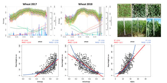
The relationship between entropy and all biophysical parameters in BBCH stages 21–49 are shown for wheat in Figure 10. Except for VWC, biophysical parameters increase exponentially with increasing entropy; therefore, the exponential regression models result in higher R2 values compared to linear models. For high entropy values (>0.7), the related biophysical parameter values are widely spread and a discrimination is not possible anymore. The good performance of plant height might be due to the comparatively low number of very small values. The RMSE values of all combinations are relatively high compared to the value range.
Figure 11 shows the scatter plots for plant height related to entropy, anisotropy, and alpha. Similar to entropy, the alpha values increase with increasing plant height, whereas anisotropy values decrease with increasing plant height. The R2 values are similar for both linear and exponential regression. The advantage of anisotropy in explaining variability in cases where entropy is high is visible as plant heights between 20 cm and 80 cm are spread over a larger range of anisotropy (around 0.1–0.7) compared to entropy (around 0.6–1). The RMSE values of all three dual-polarimetric parameters are similar (12.46–12.65), with slightly higher values of exponential models of anisotropy and alpha (13.61 and 13.89).
The regression analysis with data from BBCH stages 21–49 was additionally performed for each individual field to detect fields with consistently good regression results and fields with rather poor results (Figure 12). Most of the wheat fields reach equally high R2 values except for field A, which consistently has very poor regression results with R2 values lower than 0.1. Individual wheat fields reach very high R2 values of 0.7 and up to 0.76, for example fields G, S, E and Hey. These high R2 values are reached for exponential regression of all three polarimetric decomposition parameters combined with biomass, VWC, LAI, and plant height, whereas LAI and plant height perform best.
Only two barley fields (F and H) reach R2 values higher than 0.5, with a maximum value of 0.56 for the exponential regression of alpha and plant height for field H.
As a last step, a multiple regression including the backscatter parameters VV and VH and the polarimetric decomposition parameters entropy and alpha was performed for BBCH stages 21–49. Anisotropy was neglected because of multicollinearity with entropy. Using a stepwise approach enabled us to define the best performing model variables. All one-variable models of backscatter and polarimetric decomposition parameters are shown to compare their performance with that of the multiple model (Table 5 and Table 6).
The regression results of the multiple regression of wheat and all biophysical parameters reaches R2 higher than 0.64 and up to 0.76 except for relative VWC. Both linear and exponential regression perform similarly well. The best results achieve plant height with R2 values of 0.75 (linear) and 0.76 (exponential). The backscatter parameter VV reaches highest R2 values for the one-variable regression model and consequently contributes to all multiple models as well. Particularly, exponential multiple regression models benefit from the inclusion of further parameters, and strongest effects are observed for plant height. The R2 values are up to 0.07 higher compared to the best one-variable exponential model, and linear models slightly improve their R2 values but are not higher than around 0.04. Considering both exponential and linear models, R2 values of multiple regression improve by up to 0.05 for plant height. Most exponential multiple models include all four variables, whereas linear models mostly consist of two or three variables. RMSE values of multiple regression models are lower than those of one-variable models, for example, 9.2 cm compared to higher than 12 cm for plant height, 0.98 compared to higher than 1.2 for LAI, or 625 g/m2 compared to higher than 800 g/m2 for wet biomass.
For barley, VV backscatter provides the best regression results for the one-variable models as well, but R2 are lower than these for wheat (Table 6). Multiple regression models of plant height reach the highest R2 values but do not exceed 0.65, whereas multiple regression models of biomass, VWC, and LAI reach R2 values in the range of 0.41 to 0.47. Multiple regression models improve the R2 values only slightly, the difference in R2 values of the one-variable model of VV backscatter, and the multiple model is up to 0.06 for VWC. In contrast to wheat, linear models yield better (particularly wet and dry biomass) or equal R2 values than exponential models. Models predicting relative VWC reach higher R2 values for barley (0.33) than for wheat (0.26).
Exponential multiple regression models predicting plant height for wheat and barley are exemplarily applied for the Blönsdorf fields observed in 2018 using Equation (13) for wheat and Equation (14) for barley (Figure 13). The resulting maps of four dates during BBCH stages 21–49 represent the plant development in the course of the vegetation period starting with plant heights around 10 cm in March. With the beginning of the stem elongation in April, plant growth increased remarkably. At the end of April, fields E, F, and G had plant heights around 40 cm whereas field H already reached plant heights around 60 cm, which was also observed during the field measurements (Figure 4). In May, plant heights between 40 and 60 cm were reached for wheat, which is consistent with observed heights in the field. For field F, the model overestimates plant height and suggests heights from 60 to 80 cm, whereas heights only up to 60 cm were measured in the field. Field heterogeneity can only be observed at the end of April for field H.
6. Discussion
Analysis of the temporal behavior as well as of regression models using polarimetric decomposition parameters entropy, anisotropy, and alpha is both helpful in enhancing the understanding of these parameters regarding their ability to enable agricultural monitoring.
The temporal development of polarimetric decomposition parameters in the course of the vegetation period is mainly caused by structural changes of the vegetation as well as by varying soil and vegetation contributions to the signal. The temporal profiles show recurrent trends in both years for all acquisition settings but are also sensitive to specific meteorological conditions such as intense rainfall events in 2017 or snowfall in March and April 2018 as well as summer drought, particularly in 2018. Compared to the temporal behavior of backscatter parameters, entropy, anisotropy, and alpha show similar reactions to phenological changes [12,13,14]. Both reflect the growing vegetation at the beginning of the vegetation period with decreasing or increasing values and find their maximum or minimum during the booting stage. The heading stage marks a turning point of the course, and from that time on, the parameter values increase or decrease again. An advantage of backscatter profiles is their ability to reflect the time of the bending of the heads of barley [13]. Entropy, anisotropy, and alpha profiles are not that sensitive to this structural change and the time of the bending of the heads is not observable. Similar to this study, Mercier et al. [35] also observed a highly varying polarisation during stem elongation due to heterogeneous plant structures, which was expressed by an increasing Shannon entropy.
Although there are tremendous differences between fields regarding biophysical parameters such biomass, VWC, and LAI (Figure 4), these differences are not definitely distinguishable using temporal profiles of entropy, anisotropy, and alpha. Whereas at least few differences between fields could be observed, e.g., at the beginning of the vegetation period or during ripening, within-field variability was not detectable. Furthermore, some observed between- and within-field differences are more likely to explain variability in the plant structure, leaf, or head orientation, which is not recorded by the existing field measurements. Within-field variability could not be detected using backscatter data as well, whereas between-field variability was more pronounced in backscatter data particularly for barley [13].
As a next step, the comparison of breakpoints and local extrema of a smoothed temporal profile with phenological changes would be reasonable to estimate the beginning of phenological stages such as booting, ripening. or harvest [17,18]. This information would be particularly interesting for farmers adopting their field management such as irrigation or fertilization as well as harvesting according to current phenological stages.
Additionally, the performance of regression models differs remarkably between phenological stages, which was also found by previous studies for backscatter [7,13,16]. The best results are reached in the early BBCH stages from tillering to booting (21–49) because changes in the plant appearance indicated by increasing biomass, LAI, and plant height are most evident at this time. In later BBCH stages, the biophysical parameters change slower and are more subtle. These changes, such as moisture changes in the grains or structural changes of the plants in general, are not observable by the applied measurements. Because relative VWC does not remarkably change during BBCH stages 21–49 (Figure 4), the regression models predicting this parameter perform rather poorly.
Multiple models combining backscatter parameters and polarimetric decomposition parameters improve R2 values by up to 0.05 for plant height compared to those of single regression models. Multiple regression achieves highest R2 values for plant height because this parameter is easy to measure and measurement errors are unlikely. The main reason for the good performance might be the value range. All height values are evenly distributed over the value range and do not increase as fast and steep as for example biomass values. Furthermore, many small values do not significantly influence the regression line as is the case for biomass.
Because barley plants are already higher and more dense compared to wheat plants at the beginning of the vegetation period, resulting regression models reach not as high R2 values compared to wheat. The missing of small values prevent the fitting of an exponential regression line, and the value range is smaller. This also explains the better performance of fields F and H because these fields are comparatively smaller and not as dense as other barley fields in the same period.
The polarimetric decomposition parameters of full-polarimetric SAR data such as RADARSAT-2 reach generally higher or comparably high R2 values of single parameters compared to dual-polarimetric decomposition parameters of our study. Betbeder et al. [26] used a different decomposition algorithm and calculated Shannon entropy for Sentinel-1 data, which similar to entropy derived from H-A-α decomposition describes the randomness of the scattering. They reached R2 values up to 0.7 for Shannon entropy and rapeseed height. Mercier et al. [35] calculated the Shannon entropy for Sentinel-1 data and found that it is an important parameter for predicting the phenological stages of wheat and rapeseed. Wiseman et al. [7] used a H-A-α decomposition for RADARSAT-2 data and linearly correlated entropy, anisotropy, alpha, and further SAR parameters with dry biomass of spring wheat. They reached R2 values of 0.215 for entropy and 0.418 for alpha. These values were comparable to our wheat results (0.4 for dry biomass and alpha) or lower (0.37 for dry biomass and entropy). The reasons for the comparatively lower performance of RADARSAT-2 data in this case might be that data from the whole vegetation period was used and might be furthermore due to the lower temporal resolution of RADARSAT-2. Canisius et al. [25] also used RADARSAT-2 data to correlate the biophysical parameters of spring wheat with the polarimetric decomposition parameters. They found a high correlation between wheat height and alpha angle, with an R2 value of 0.66, which is slightly higher than our R2 value of 0.6 for alpha and plant height of wheat. The R2 value of Canisius et al. [25] was even higher for a smoothed time series and reached a value of 0.88.
Similar to temporal profiles, it is not possible to detect the field variability of biophysical parameters using regression models of backscatter and polarimetric decomposition parameters of single dates. The RMSE values are too high for a meaningful estimation of biophysical parameters and are sometimes even higher than the expected variability within a field on a single date, for example, around 9 cm for plant height. Varying meteorological conditions between years make it difficult to establish generally valid regression models as well. Therefore, the identification of phenological stages, e.g., based on temporal profiles, is meaningful.
Irregular patterns in images of polarimetric parameters make it difficult to make statements about individual points and complicates the fitting of a regression model as well as the detection of between- and within-field variability. These patterns are due to the radar speckle, the "salt-and-pepper-effect" of the images, which is individual for every image. The extraction of values of a small area includes only a few pixels; therefore, the exact extraction location has a high influence on the extracted value because neighboring pixels might be extremely different. This is a general characteristic of radar images and is furthermore fostered by speckle filtering and other averaging processes such as multilooking. These processing steps affect the inherent scattering mechanisms of each pixel and a higher amount of averaging results, for instance, in increasing entropy values and decreasing anisotropy values [51]. The high spatial variability of decomposition parameters is also mentioned in other studies [29,36]. To obtain more meaningful information for individual points, a larger extraction area or a smoothed image could improve the results, but there is again the trade-off between smoothing and information loss. Further error sources might be the different quality of field measurements, geometric inaccuracies of the SAR data caused by image processing, and differing local incidence angles, among others.
In the future, the current results of dual-polarimetric decomposition of Sentinel-1 data can be compared to the decomposition parameters of full polarimetric SAR data such as RADARSAT-2. Additionally, a smoothing of the time series could lead to better regression results, as found by Canisius et al. [25]. Furthermore, the multiple regression analysis could be performed using additional parameters such as the Radar Vegetation Index (RVI) [61], Shannon entropy [35], or field statistics of SAR parameters, as was done by Holtgrave et al. [16]. Additionally, it would be advantageous if existing field measurements are completed by additional parameters with the consideration of water content in different parts of the plant to catch also small water content differences, particularly during the ripening in the grains. Furthermore, the documentation of structural changes such as the emergence of flag leaves or heads as well as the bending of the heads must be documented in detail to explain scattering changes.
7. Conclusions
This study confirms that the polarimetric decomposition parameters of the dual-polarimetric Sentinel-1 data are useful for the monitoring of biophysical parameters on agricultural fields with some limitations. Temporal profiles of entropy, anisotropy, and alpha are sensitive to changes in the plant appearance in the course of the phenological development of both wheat and barley, whereas the variable contribution of soil and vegetation as well as the changing water content of the plants mainly influence the SAR signal. Furthermore, differences between the two years 2017, which was rather wet, and 2018, a very dry year, are clearly evident in the temporal profiles. However, temporal profiles of individual fields do not satisfactorily reflect differences between and within fields caused by varying biophysical parameters.
Regression models of polarimetric decomposition parameters related to biophysical parameters show particularly high R2 values for wheat in BBCH stages 21–49 (tillering to booting). Plant height could be predicted using single exponential regression models of entropy and anisotropy with R2 of 0.64 and 0.61, respectively. Multiple regression models including entropy and alpha as well as backscatter coefficients VH and VV resulted in even higher R2 values for plant height (0.76), wet biomass (0.7), dry biomass (0.7), and vegetation water content (0.69). Therefore, polarimetric decomposition parameters are beneficial as additional input parameters for multiple regression models to improve the prediction of biophysical parameters. The R2 values of multiple regression models improved by up to 0.05 by taking the dual-polarimetric parameters into account compared to using only backscatter parameters. Furthermore, the RMSE values are around 10% and up to 20% lower compared to those of single regression models but are still too high for a meaningful prediction of biophysical parameters on single dates.
The presented results serve as a basis for further research in agricultural monitoring and show the potential of polarimetric decomposition parameters of Sentinel-1 data as an additional source of information next to backscatter coefficients.
Author Contributions
Conceptualization, K.H., S.I., D.S., and C.W.; methodology, K.H.; formal analysis, K.H.; investigation, K.H.; data curation, K.H.; writing—original draft preparation, K.H.; writing—review and editing, K.H., S.I., D.S., and C.W.; visualization, K.H.; supervision, S.I., D.S., and C.W.; project administration, D.S.; funding acquisition, D.S. All authors have read and agreed to the published version of the manuscript.
Funding
This research is funded by the Federal Ministry of Food and Agriculture (BMEL) based on a decision of the Parliament of the Federal Republic of Germany via the Federal Office for Agriculture and Food (BLE) under the innovation support programme, grant number 2815710715.
Data Availability Statement
Publicly available datasets were analyzed in this study. Sentinel-1 data can be found here: https://scihub.copernicus.eu/. Field data and resulting data sets presented in this study are available on request from the corresponding author.
Acknowledgments
The authors would like to thank numerous interns and students for their great support in the fieldwork.
Conflicts of Interest
The authors declare no conflict of interest. The funders had no role in the design of the study; in the collection, analyses, or interpretation of data; in the writing of the manuscript; or in the decision to publish the results.
References
- Mc Nairn, H.; Brisco, B. The application of C-band polarimetric SAR for agriculture: A review. Can. J. Remote. Sens. 2004, 30, 525–542. [Google Scholar] [CrossRef]
- Steele-Dunne, S.C.; McNairn, H.; Monsivais-Huertero, A.; Mahdian, M.; Homayouni, S.; Fazel, M.A.; Mohammadimanesh, F.; Baghdadi, N.; Cresson, R.; El Hajj, M.; et al. Radar Remote Sensing of Agricultural Canopies: A Review. Remote Sens. Environ. 2016, 187, 1607–1621. [Google Scholar] [CrossRef] [Green Version]
- Satalino, G.; Balenzano, A.; Mattia, F.; Davidson, M.W. C-band SAR data for mapping crops dominated by surface or volume scattering. IEEE Geosci. Remote Sens. Lett. 2014, 11, 384–388. [Google Scholar] [CrossRef]
- Skriver, H.; Mattia, F.; Satalino, G.; Balenzano, A.; Pauwels, V.R.N.; Verhoest, N.E.C.; Davidson, M. Crop Classification Using Short-Revisit Multitemporal SAR Data. IEEE J. Sel. Top. Appl. Earth Obs. Remote Sens. 2011, 4, 423–431. [Google Scholar] [CrossRef]
- Bargiel, D. A new method for crop classification combining time series of radar images and crop phenology information. Remote Sens. Environ. 2017, 198, 369–383. [Google Scholar] [CrossRef]
- Macelloni, G.; Paloscia, S.; Pampaloni, P.; Marliani, F.; Gai, M. The relationship between the backscattering coefficient and the biomass of narrow and broad leaf crops. IEEE Trans. Geosci. Remote Sens. 2001, 39, 873–884. [Google Scholar] [CrossRef]
- Wiseman, G.; McNairn, H.; Homayouni, S.; Shang, J. RADARSAT-2 Polarimetric SAR response to crop biomass for agricultural production monitoring. IEEE J. Sel. Top. Appl. Earth Obs. Remote Sens. 2014, 7, 4461–4471. [Google Scholar] [CrossRef]
- Inoue, Y.; Sakaiya, E.; Wang, C. Capability of C-band backscattering coefficients from high-resolution satellite SAR sensors to assess biophysical variables in paddy rice. Remote Sens. Environ. 2014, 140, 257–266. [Google Scholar] [CrossRef]
- Vicente-Guijalba, F.; Martinez-Marin, T.; Lopez-Sanchez, J.M. Dynamical approach for real-time monitoring of agricultural crops. IEEE Trans. Geosci. Remote Sens. 2015, 53, 3278–3293. [Google Scholar] [CrossRef] [Green Version]
- Susan Moran, M.; Alonso, L.; Moreno, J.F.; Pilar Cendrero Mateo, M.; Fernando de la Cruz, D.; Montoro, A.; Alonso, L.; Moreno, J.F.; Cendrero Mateo, M.P. A RADARSAT-2 Quad-Polarized Time Series for Monitoring Crop and Soil Conditions in Barrax, Spain Biological Resource Management for Sustainable Agricultural Systems to encourage international research on sustainable use of natural resources in agriculture. Ieee Trans. Geosci. Remote Sens. 2011, 1, 1–14. [Google Scholar] [CrossRef]
- Skriver, H.; Svendsen, M.T.; Thomsen, A.G. Multitemporal C- and L-band polarimetric signatures of crops. IEEE Trans. Geosci. Remote Sens. 1999, 37, 2413–2429. [Google Scholar] [CrossRef]
- Vreugdenhil, M.; Wagner, W.; Bauer-Marschallinger, B.; Pfeil, I.; Teubner, I.; Rüdiger, C.; Strauss, P. Sensitivity of Sentinel-1 backscatter to vegetation dynamics: An Austrian case study. Remote Sens. 2018, 10, 1396. [Google Scholar] [CrossRef] [Green Version]
- Harfenmeister, K.; Spengler, D.; Weltzien, C. Analyzing Temporal and Spatial Characteristics of Crop Parameters Using Sentinel-1 Backscatter Data. Remote Sens. 2019, 11, 1569. [Google Scholar] [CrossRef] [Green Version]
- Veloso, A.; Mermoz, S.; Bouvet, A.; Le Toan, T.; Planells, M.; Dejoux, J.F.; Ceschia, E. Understanding the temporal behavior of crops using Sentinel-1 and Sentinel-2-like data for agricultural applications. Remote Sens. Environ. 2017, 199, 415–426. [Google Scholar] [CrossRef]
- Khabbazan, S.; Vermunt, P.; Steele-Dunne, S.; Ratering Arntz, L.; Marinetti, C.; van der Valk, D.; Iannini, L.; Molijn, R.; Westerdijk, K.; van der Sande, C. Crop Monitoring Using Sentinel-1 Data: A Case Study from The Netherlands. Remote Sens. 2019, 11, 1887. [Google Scholar] [CrossRef] [Green Version]
- Holtgrave, A.K.; Röder, N.; Ackermann, A.; Erasmi, S.; Kleinschmit, B. Comparing Sentinel-1 and -2 data and indices for agricultural land use monitoring. Remote Sens. 2020, 12, 2919. [Google Scholar] [CrossRef]
- Schlund, M.; Erasmi, S. Sentinel-1 time series data for monitoring the phenology of winter wheat. Remote Sens. Environ. 2020, 246, 111814. [Google Scholar] [CrossRef]
- Nasrallah, A.; Baghdadi, N.; El Hajj, M.; Darwish, T.; Belhouchette, H.; Faour, G.; Darwich, S.; Mhawej, M. Sentinel-1 data for winter wheat phenology monitoring and mapping. Remote Sens. 2019, 11, 2228. [Google Scholar] [CrossRef] [Green Version]
- Hajnsek, I.; Jagdhuber, T.; Schön, H.; Papathanassiou, K.P. Potential of estimating soil moisture under vegetation cover by means of PolSAR. IEEE Trans. Geosci. Remote Sens. 2009, 47, 442–454. [Google Scholar] [CrossRef] [Green Version]
- Jagdhuber, T.; Hajnsek, I.; Bronstert, A.; Papathanassiou, K.P. Soil moisture estimation under low vegetation cover using a multi-angular polarimetric decomposition. IEEE Trans. Geosci. Remote Sens. 2013, 51, 2201–2215. [Google Scholar] [CrossRef]
- Wang, H.; Magagi, R.; Goita, K. Comparison of different polarimetric decompositions for soil moisture retrieval over vegetation covered agricultural area. Remote Sens. Environ. 2017, 199, 120–136. [Google Scholar] [CrossRef]
- McNairn, H.; Shang, J.; Jiao, X.; Champagne, C. The contribution of ALOS PALSAR multipolarization and polarimetric data to crop classification. IEEE Trans. Geosci. Remote Sens. 2009, 47, 3981–3992. [Google Scholar] [CrossRef] [Green Version]
- Jiao, X.; Kovacs, J.M.; Shang, J.; McNairn, H.; Walters, D.; Ma, B.; Geng, X. Object-oriented crop mapping and monitoring using multi-temporal polarimetric RADARSAT-2 data. ISPRS J. Photogramm. Remote Sens. 2014, 96, 38–46. [Google Scholar] [CrossRef]
- Mascolo, L.; Lopez-Sanchez, J.M.; Vicente-Guijalba, F.; Nunziata, F.; Migliaccio, M.; Mazzarella, G. A Complete Procedure for Crop Phenology Estimation with PolSAR Data Based on the Complex Wishart Classifier. IEEE Trans. Geosci. Remote Sens. 2016, 54, 6505–6515. [Google Scholar] [CrossRef] [Green Version]
- Canisius, F.; Shang, J.; Liu, J.; Huang, X.; Ma, B.; Jiao, X.; Geng, X.; Kovacs, J.M.; Walters, D. Tracking crop phenological development using multi-temporal polarimetric Radarsat-2 data. Remote Sens. Environ. 2018, 210, 508–518. [Google Scholar] [CrossRef]
- Betbeder, J.; Fieuzal, R.; Philippets, Y.; Ferro-Famil, L.; Baup, F. Contribution of multitemporal polarimetric synthetic aperture radar data for monitoring winter wheat and rapeseed crops. J. Appl. Remote Sens. 2016, 10, 026020. [Google Scholar] [CrossRef]
- Ji, K.; Wu, Y. Scattering Mechanism Extraction by a Modified Cloude-Pottier Decomposition for Dual Polarization SAR. Remote Sens. 2015, 7, 7447–7470. [Google Scholar] [CrossRef] [Green Version]
- Cloude, S.R. The dual polarisation entropy/alpha decomposition: A PALSAR case study. Sci. Appl. Sar Polarim. Polarim. Interferom. 2007, 644, 2. [Google Scholar]
- Engelbrecht, J.; Theron, A.; Vhengani, L.; Kemp, J. A simple normalized difference approach to burnt area mapping using multi-polarisation C-Band SAR. Remote Sens. 2017, 9, 764. [Google Scholar] [CrossRef] [Green Version]
- Plank, S.; Jüssi, M.; Martinis, S.; Twele, A. Mapping of flooded vegetation by means of polarimetric sentinel-1 and ALOS-2/PALSAR-2 imagery. Int. J. Remote. Sens. 2017, 38, 3831–3850. [Google Scholar] [CrossRef]
- Velotto, D.; Bentes, C.; Tings, B.; Lehner, S. First Comparison of Sentinel-1 and TerraSAR-X Data in the Framework of Maritime Targets Detection: South Italy Case. IEEE J. Ocean. Eng. 2016, 41, 993–1006. [Google Scholar] [CrossRef]
- Banqué, X.; Lopez-Sanchez, J.M.; Monells, D.; Ballester, D.; Duro, J. Polarimetry-Based Land Cover Classification with Sentinel-1 Data. Polinsar 2015, 729, 1–5. [Google Scholar]
- Li, M.; Bijker, W. Vegetable classification in Indonesia using Dynamic Time Warping of Sentinel-1A dual polarization SAR time series. Int. J. Appl. Earth Obs. Geoinf. 2019, 78, 268–280. [Google Scholar] [CrossRef]
- Chauhan, S.; Darvishzadeh, R.; Boschetti, M.; Nelson, A. Discriminant analysis for lodging severity classification in wheat using RADARSAT-2 and Sentinel-1 data. ISPRS J. Photogramm. Remote. Sens. 2020, 164, 138–151. [Google Scholar] [CrossRef]
- Mercier, A.; Betbeder, J.; Baudry, J.; Le Roux, V.; Spicher, F.; Lacoux, J.; Roger, D.; Hubert-Moy, L. Evaluation of Sentinel-1 & 2 time series for predicting wheat and rapeseed phenological stages. ISPRS J. Photogramm. Remote. Sens. 2020, 163, 231–256. [Google Scholar] [CrossRef]
- Heine, I.; Jagdhuber, T.; Itzerott, S. Classification and monitoring of reed belts using dual-polarimetric TerraSAR-X time series. Remote Sens. 2016, 8, 552. [Google Scholar] [CrossRef] [Green Version]
- Voormansik, K.; Jagdhuber, T.; Zalite, K.; Noorma, M.; Hajnsek, I. Observations of Cutting Practices in Agricultural Grasslands Using Polarimetric SAR. IEEE J. Sel. Top. Appl. Earth Obs. Remote Sens. 2016, 9, 1382–1396. [Google Scholar] [CrossRef]
- Lopez-Sanchez, J.M.; Cloude, S.R.; Ballester-Berman, J.D. Rice phenology monitoring by means of SAR polarimetry at X-band. IEEE Trans. Geosci. Remote Sens. 2012, 50, 2695–2709. [Google Scholar] [CrossRef]
- Ratzke, U.; Mohr, H.J. Böden in Mecklenburg-Vorpommern: Abriss ihrer Entstehung, Verbreitung und Nutzung; Beiträge zum Bodenschutz in Mecklenburg-Vorpommern, Landesamt für Umwelt, Naturschutz und Geologie Mecklenburg-Vorpommern: Güstrow, Germany, 2003. [Google Scholar]
- Spengler, D.; Förster, M.; Borg, E. Editorial. PFG-J. Photogramm. Remote. Sens. Geoinf. Sci. 2018, 86, 49–51. [Google Scholar] [CrossRef] [Green Version]
- Zacharias, S.; Bogena, H.; Samaniego, L.; Mauder, M.; Fuß, R.; Pütz, T.; Frenzel, M.; Schwank, M.; Baessler, C.; Butterbach-Bahl, K.; et al. A Network of Terrestrial Environmental Observatories in Germany. Vadose Zone J. 2011, 10, 955–973. [Google Scholar] [CrossRef] [Green Version]
- Heinrich, I.; Balanzategui, D.; Bens, O.; Blasch, G.; Blume, T.; Böttcher, F.; Borg, E.; Brademann, B.; Brauer, A.; Conrad, C.; et al. Interdisciplinary Geo-ecological Research across Time Scales in the Northeast German Lowland Observatory (TERENO-NE). Vadose Zone J. 2018, 17, 1–25. [Google Scholar] [CrossRef] [Green Version]
- Amt für Statistik Berlin-Brandenburg. Statistischer Bericht C I 1–j/17. Bodennutzung der Landwirtschaftlichen Betriebe im Land Brandenburg 2017; Amt für Statistik Berlin-Brandenburg: Potsdam, Germany, 2017. [Google Scholar]
- Amt für Statistik Berlin-Brandenburg. Statistischer Bericht C I 1–j/18. Bodennutzung der Landwirtschaftlichen Betriebe im Land Brandenburg 2018; Amt für Statistik Berlin-Brandenburg: Potsdam, Germany, 2018. [Google Scholar]
- Ministerium für Landwirtschaft und Umwelt Mecklenburg-Vorpommern. Statistisches Datenblatt 2020; Ministerium für Landwirtschaft und Umwelt Mecklenburg-Vorpommern: Schwerin, Germany, 2020.
- DWD Climate Data Center (CDC). Historical Daily Precipitation Observations for Germany, Version v007; Deutscher Wetterdienst: Offenbach, Germany, 2020. [Google Scholar]
- Eckelmann, W.; Sponagel, H.; Grottenthaler, W.; Hartmann, K.J.; Hartwich, R.; Janetzko, P.; Joisten, H.; Kühn, D.; Sabel, K.J.; Traidl, R. Bodenkundliche Kartieranleitung. KA5; Schweizerbart’sche Verlagsbuchhandlung: Stuttgart, Germany, 2005. [Google Scholar]
- Meier, U.; Bleiholder, H.; Buhr, L.; Feller, C.; Hack, H.; Heß, M.; Lancashire, P.; Schnock, U.; Stauß, R.; Van den Boom, T.; et al. The BBCH system to coding the phenological growth stages of plants-history and publications. J. Für Kult. 2009, 61, 41–52. [Google Scholar]
- Itzerott, S.; Hohmann, C.; Stender, V.; Maass, H.; Borg, E.; Renke, F.; Jahncke, D.; Berg, M.; Conrad, C.; Spengler, D. TERENO (Northeast), Climate Station Heydenhof, Germany. V. 2.0 GFZ Data Services. 2018. Available online: https://dataservices.gfz-potsdam.de/tereno-new/showshort.php?id=escidoc:3311065 (accessed on 28 December 2020).
- Russelle, M.P.; Wilhelm, W.W.; Olson, R.A.; Power, J.F. Growth Analysis Based on Degree Days. Crop Sci. 1984, 24, 28–32. [Google Scholar] [CrossRef] [Green Version]
- Lee, J.S.; Pottier, E. Polarimetric Radar Imaging: From Basics to Applications; CRC Press: Boca Raton, FL, USA, 2009. [Google Scholar] [CrossRef]
- Moreira, A.; Prats-Iraola, P.; Younis, M.; Krieger, G.; Hajnsek, I.; Papathanassiou, K.P. A tutorial on synthetic aperture radar. IEEE Geosci. Remote. Sens. Mag. 2013, 1, 6–43. [Google Scholar] [CrossRef] [Green Version]
- Cloude, S.R.; Pottier, E. An entropy based classification scheme for land applications of polarimetric SAR. IEEE Trans. Geosci. Remote. Sens. 1997, 35, 68–78. [Google Scholar] [CrossRef]
- ESA. SNAP—ESA Sentinel Application Platform v6.0.6. 2018. Available online: https://step.esa.int/main/snap-6-0-released/ (accessed on 28 December 2020).
- Lee, J.S.; Grunes, M.R.; de Grandi, G. Polarimetric SAR speckle filtering and its implication for classification. IEEE Trans. Geosci. Remote Sens. 1999, 37, 2363–2373. [Google Scholar] [CrossRef]
- Pottier, E.; Ferro-Famil, L. PolSARPro V5.0: An ESA educational toolbox used for self-education in the field of POLSAR and POL-INSAR data analysis. In Proceedings of the International Geoscience and Remote Sensing Symposium (IGARSS), Munich, Germany, 22–27 July 2012. [Google Scholar] [CrossRef]
- Bahrenberg, G.; Giese, E.; Mevenkamp, N.; Nipper, J. Statistische Methoden in der Geographie-Band 2: Multivariate Statistik; Schweizerbart’sche Verlagsbuchhandlung: Stuttgart, Germany, 2008. [Google Scholar]
- Kuhn, M. Caret: Classification and Regression Training. R Package Version 6.0-86. 2020. Available online: https://cran.r-project.org/web/packages/caret/index.html (accessed on 28 December 2020).
- Robinson, C.; Schumacker, R.E. Interaction effects: Centering, variance inflation factor, and interpretation issues. Mult. Linear Regres. Viewpoints 2009, 35, 6–11. [Google Scholar]
- Joerg, H.; Pardini, M.; Hajnsek, I.; Papathanassiou, K.P. Sensitivity of SAR Tomography to the Phenological Cycle of Agricultural Crops at X-, C-, and L-band. IEEE J. Sel. Top. Appl. Earth Obs. Remote Sens. 2018, 11, 3014–3029. [Google Scholar] [CrossRef]
- Mandal, D.; Kumar, V.; Ratha, D.; Dey, S.; Bhattacharya, A.; Lopez-Sanchez, J.M.; McNairn, H.; Rao, Y.S. Dual polarimetric radar vegetation index for crop growth monitoring using sentinel-1 SAR data. Remote Sens. Environ. 2020, 247, 111954. [Google Scholar] [CrossRef]
Figure 1.
Location of the two test sites DEMMIN (durable environmental multidisciplinary monitoring information network) and Blönsdorf in Germany (left) and observed wheat and barley fields with observation points in 2017 and 2018 in Demmin (center) and Blönsdorf (right): background colors of the field names indicate the year of observation.

Figure 2.
Sentinel-1 acquisitions and field measurement dates 2017 and 2018: the data gaps resulted from unavailable images at the time of analysis.
Figure 2.
Sentinel-1 acquisitions and field measurement dates 2017 and 2018: the data gaps resulted from unavailable images at the time of analysis.

Figure 3.
Characteristic appearance of wheat and barley in different BBCH (Biologische Bundesanstalt, Bundessortenamt, und CHemische Industrie) stages.
Figure 3.
Characteristic appearance of wheat and barley in different BBCH (Biologische Bundesanstalt, Bundessortenamt, und CHemische Industrie) stages.

Figure 4.
Temporal development of crop parameters for all wheat fields (A) and barley fields (B): the greenish and brownish bars between the plots represent the BBCH stages in 2017 (lower bar) and 2018 (upper bar).
Figure 4.
Temporal development of crop parameters for all wheat fields (A) and barley fields (B): the greenish and brownish bars between the plots represent the BBCH stages in 2017 (lower bar) and 2018 (upper bar).

Figure 5.
Exemplary extraction area of 176.7 m2 with the four relevant 10 m × 10 m pixels of synthetic aperture radar (SAR) data depicted in the background: the center of the circle represents the centroid of the observation points of all dates (grey dots).
Figure 5.
Exemplary extraction area of 176.7 m2 with the four relevant 10 m × 10 m pixels of synthetic aperture radar (SAR) data depicted in the background: the center of the circle represents the centroid of the observation points of all dates (grey dots).

Figure 6.
Temporal development of decomposition parameters entropy, anisotropy, and alpha for all wheat fields in 2017 (left) and 2018 (right): polygons around the lines indicate ±one standard deviation. Blue bars represent the daily precipitation sums, red lines show the cumulative growing degree days, and green lines represent soil moisture at both test sites.

Figure 7.
Temporal development of decomposition parameters entropy, anisotropy, and alpha for all barley fields in 2017 (left) and 2018 (right): polygons around the lines indicate ±one standard deviation. Blue bars represent the daily precipitation sums, red lines show the cumulative growing degree days, and green lines represent soil moisture at both test sites.

Figure 8.
Temporal development of the coefficients of variation for all polarimetric and backscatter parameters: exemplarily shown are the mean values for barley fields 2018.
Figure 8.
Temporal development of the coefficients of variation for all polarimetric and backscatter parameters: exemplarily shown are the mean values for barley fields 2018.

Figure 9.
Temporal development of decomposition parameters entropy, anisotropy, and alpha for all observed wheat fields (left) and all observed barley fields (right).
Figure 9.
Temporal development of decomposition parameters entropy, anisotropy, and alpha for all observed wheat fields (left) and all observed barley fields (right).

Figure 10.
Scatter plots of entropy and biophysical parameters of wheat for BBCH stages 21–49: the regression lines, R2, and root mean square error (RMSE) are shown in red (linear regression) and blue (exponential regression).
Figure 10.
Scatter plots of entropy and biophysical parameters of wheat for BBCH stages 21–49: the regression lines, R2, and root mean square error (RMSE) are shown in red (linear regression) and blue (exponential regression).

Figure 11.
Scatter plots of entropy, anisotropy, and alpha related to the plant height of wheat for BBCH stages 21–49: the regression lines, R2, and RMSE are shown in red (linear regression) and blue (exponential regression).
Figure 11.
Scatter plots of entropy, anisotropy, and alpha related to the plant height of wheat for BBCH stages 21–49: the regression lines, R2, and RMSE are shown in red (linear regression) and blue (exponential regression).

Figure 12.
Bar plots of R2 values of regression between crop and dual-polarimetric parameters per crop type for single fields in BBCH stages 21–49.
Figure 12.
Bar plots of R2 values of regression between crop and dual-polarimetric parameters per crop type for single fields in BBCH stages 21–49.

Figure 13.
Plant heights of four dates during BBCH stages 21–49 in 2018 estimated by multiple exponential regression for the Blönsdorf fields E and G (wheat) and F and H (barley).
Figure 13.
Plant heights of four dates during BBCH stages 21–49 in 2018 estimated by multiple exponential regression for the Blönsdorf fields E and G (wheat) and F and H (barley).


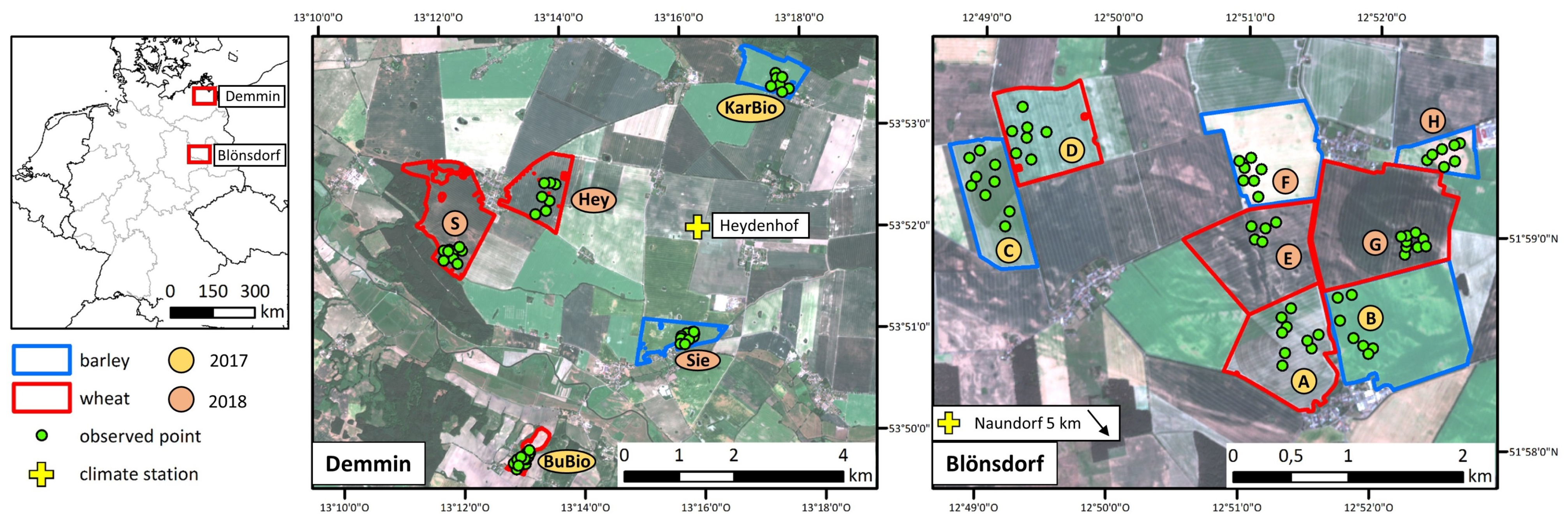
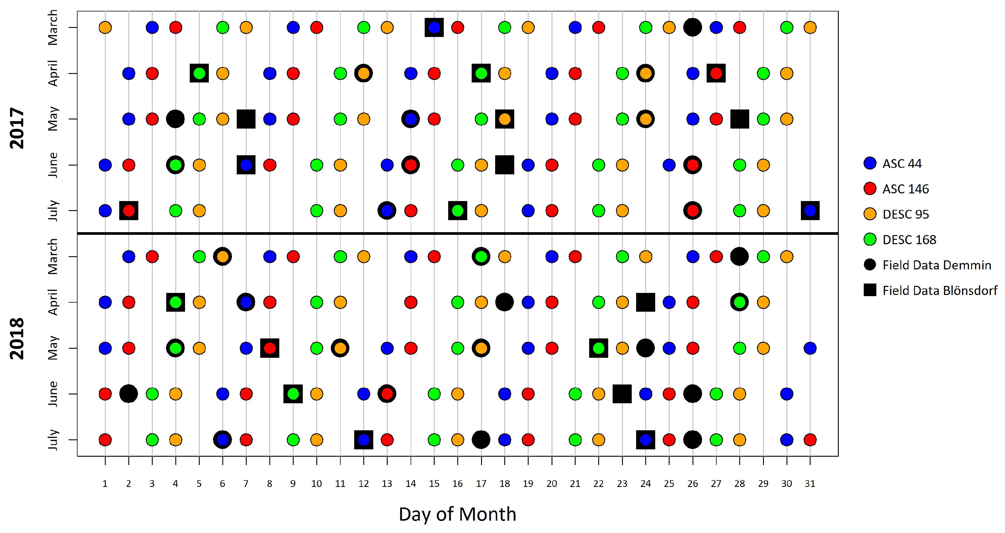
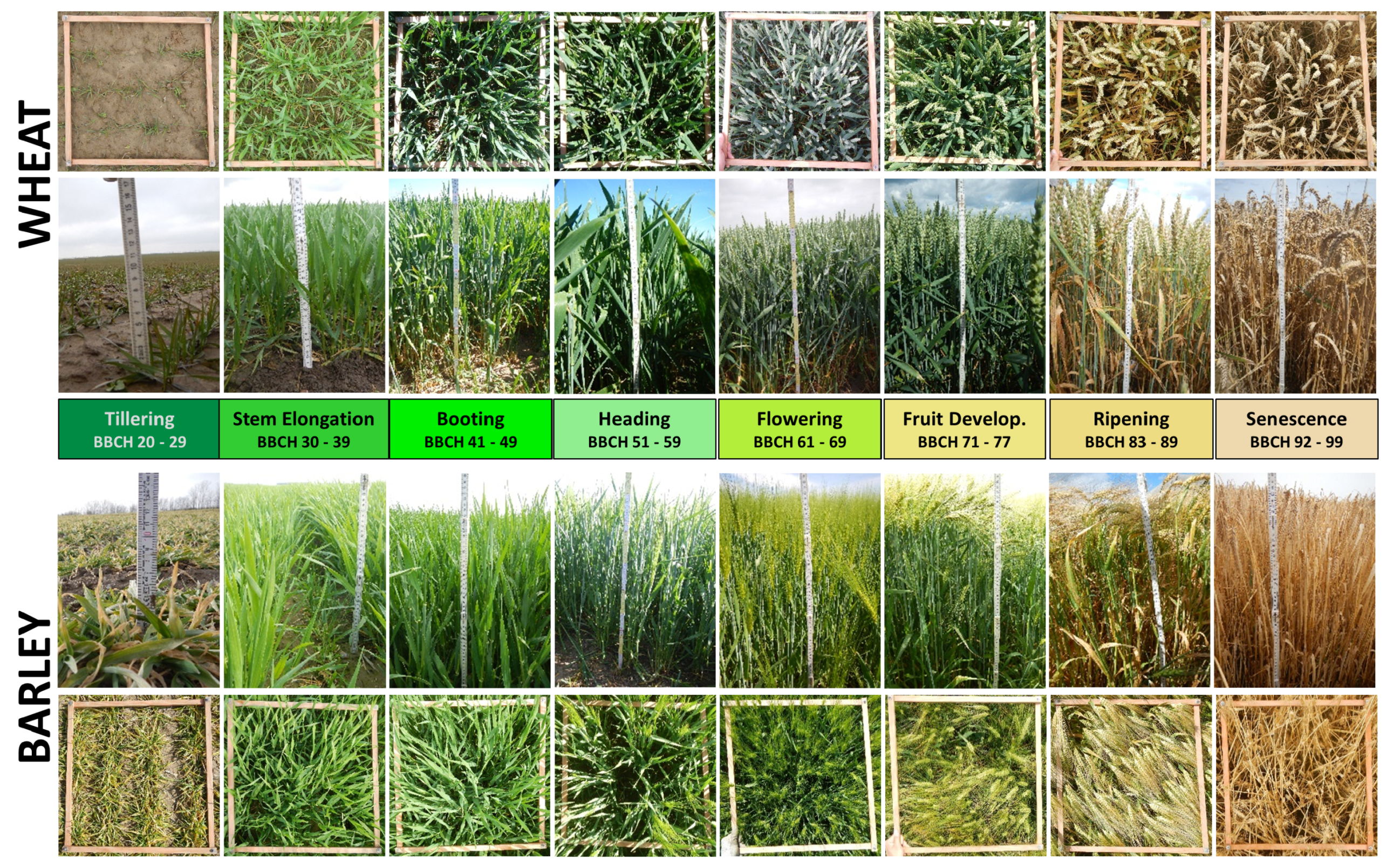
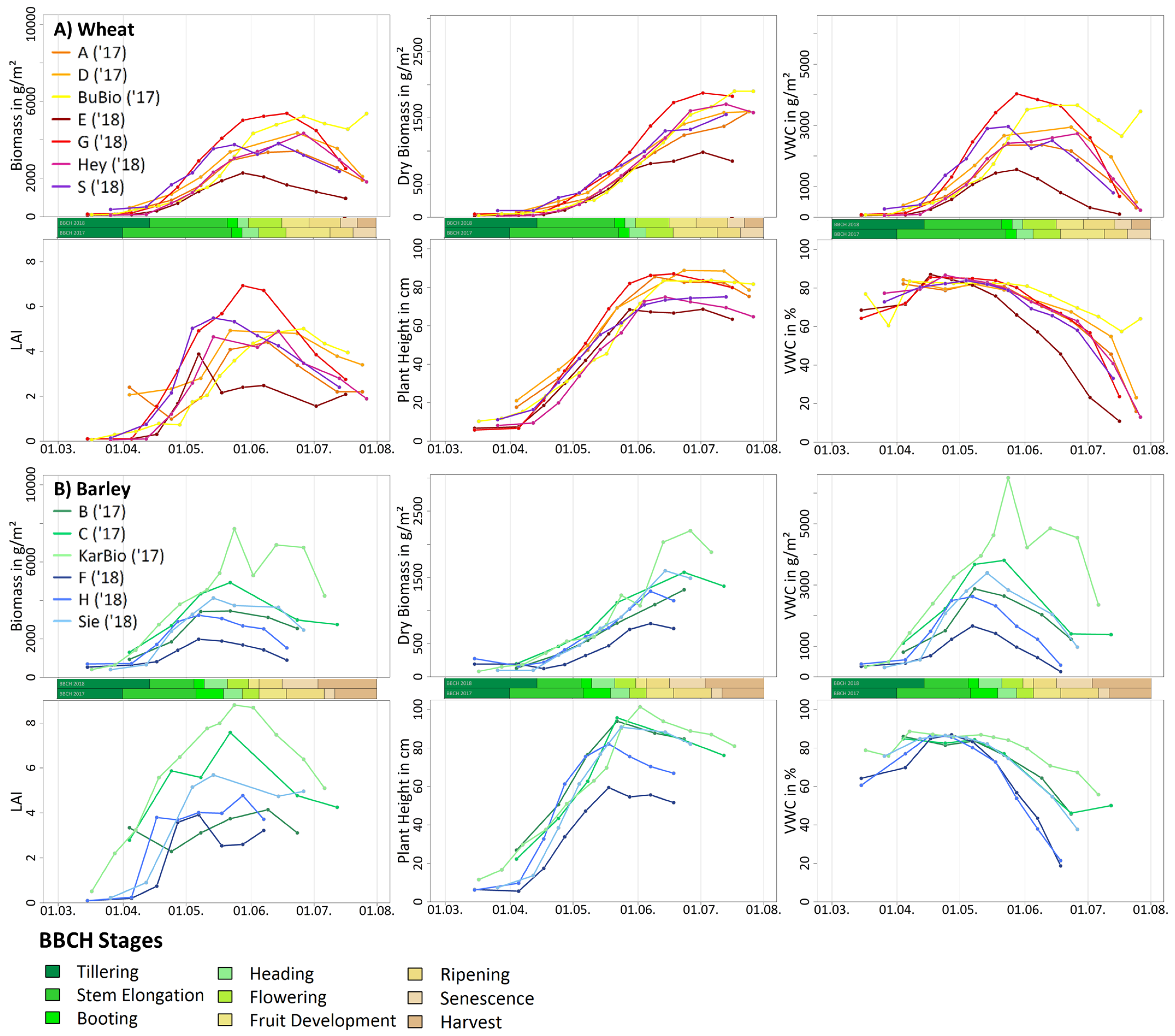
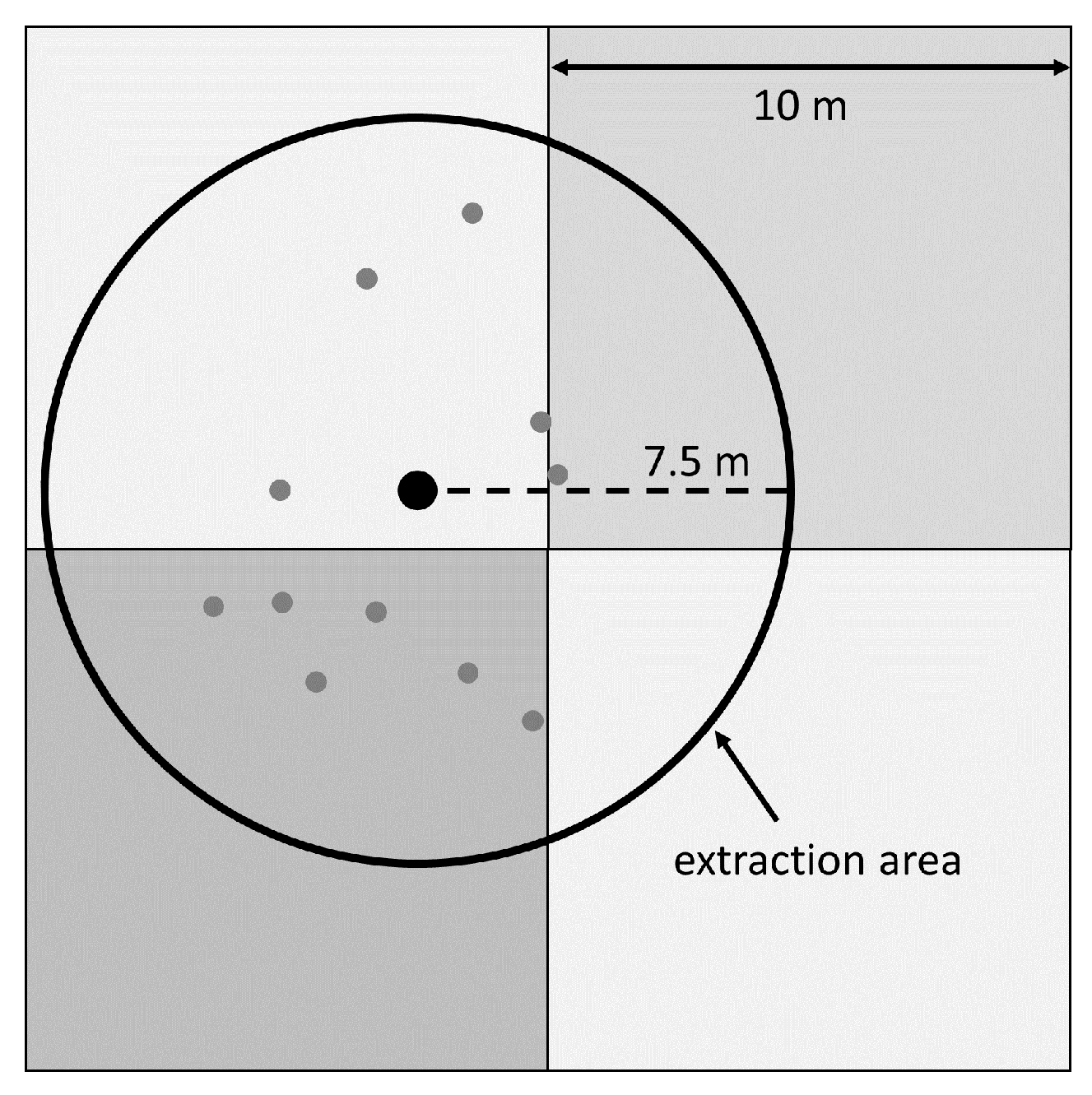
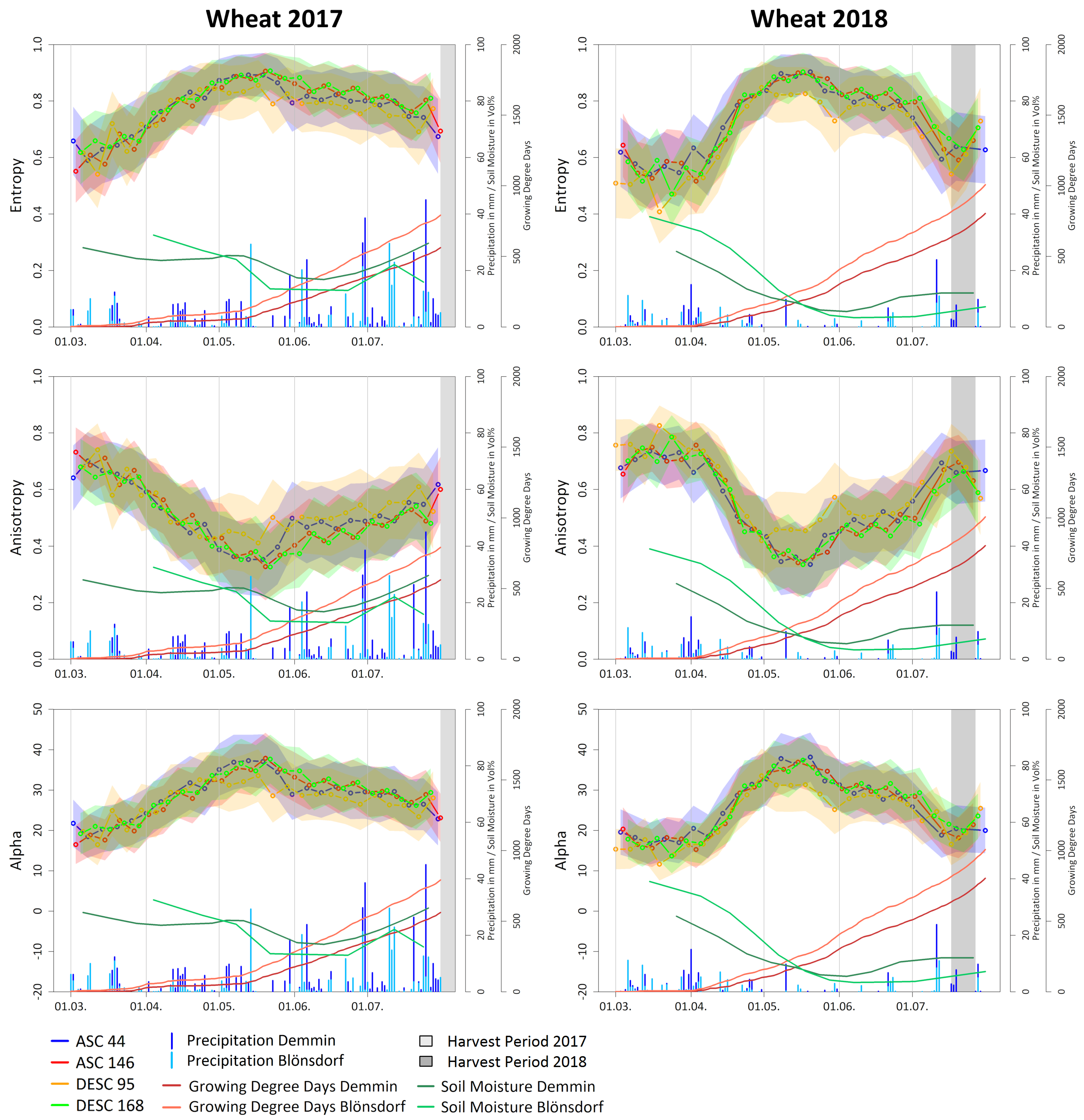
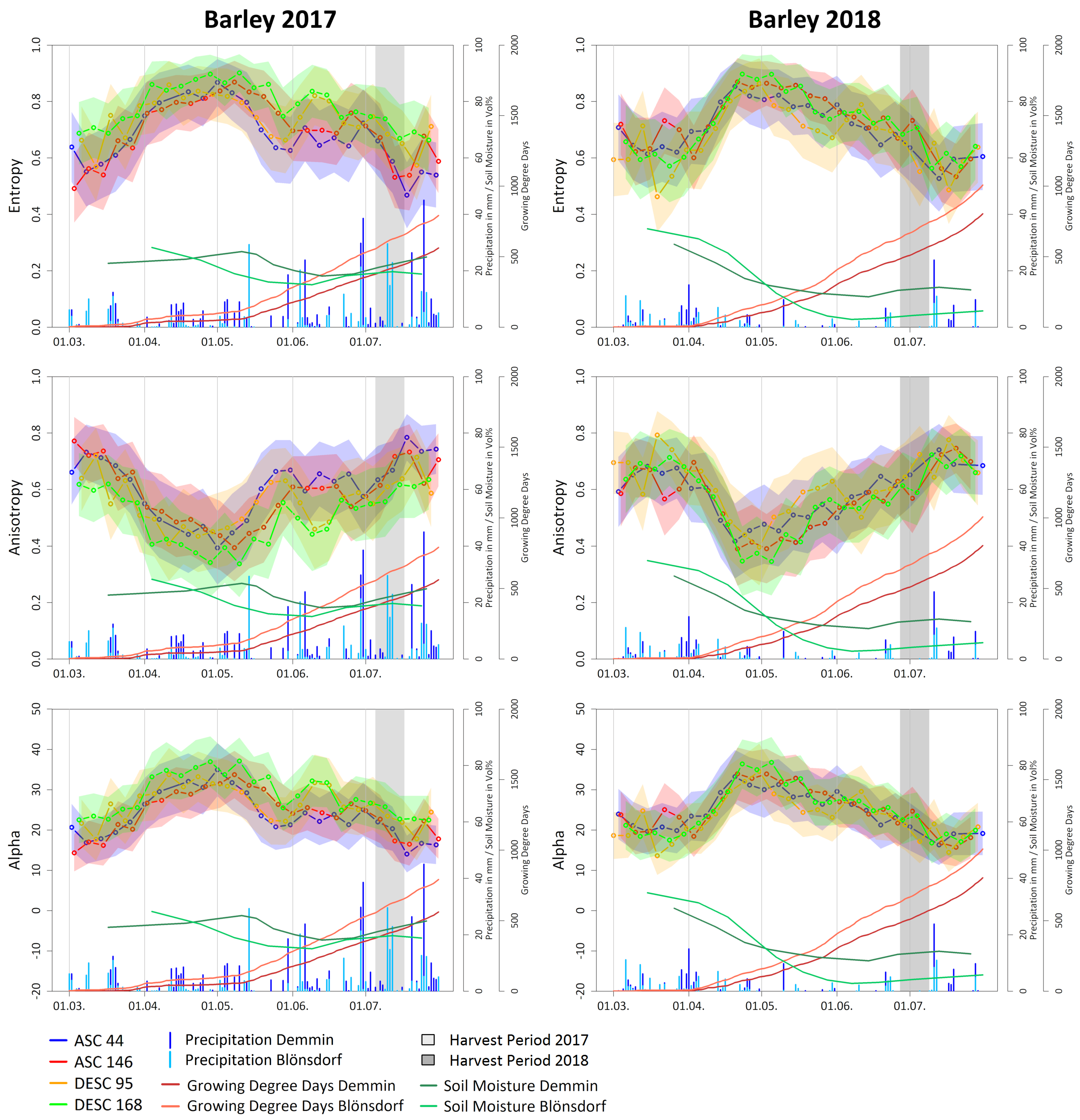
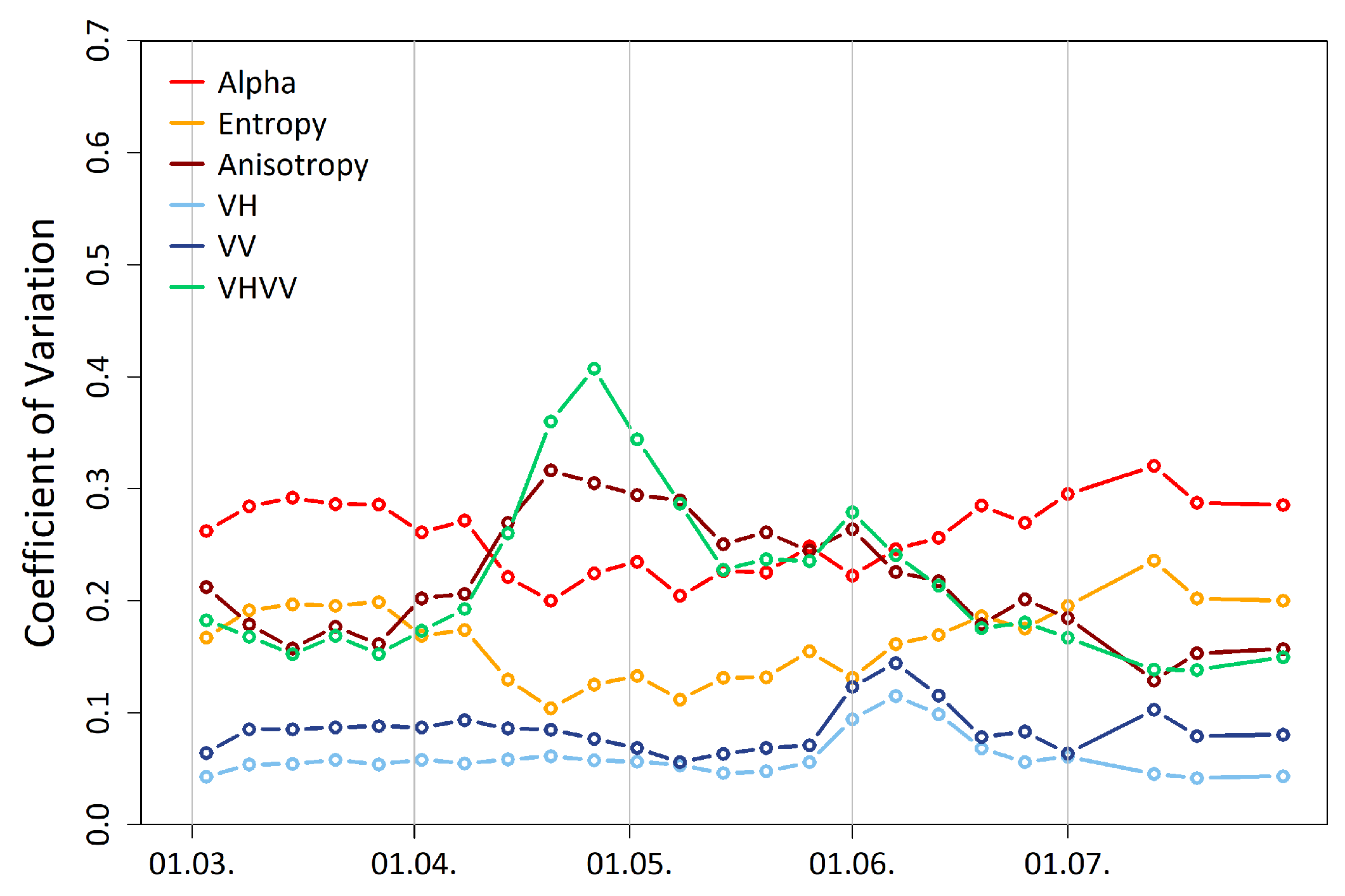
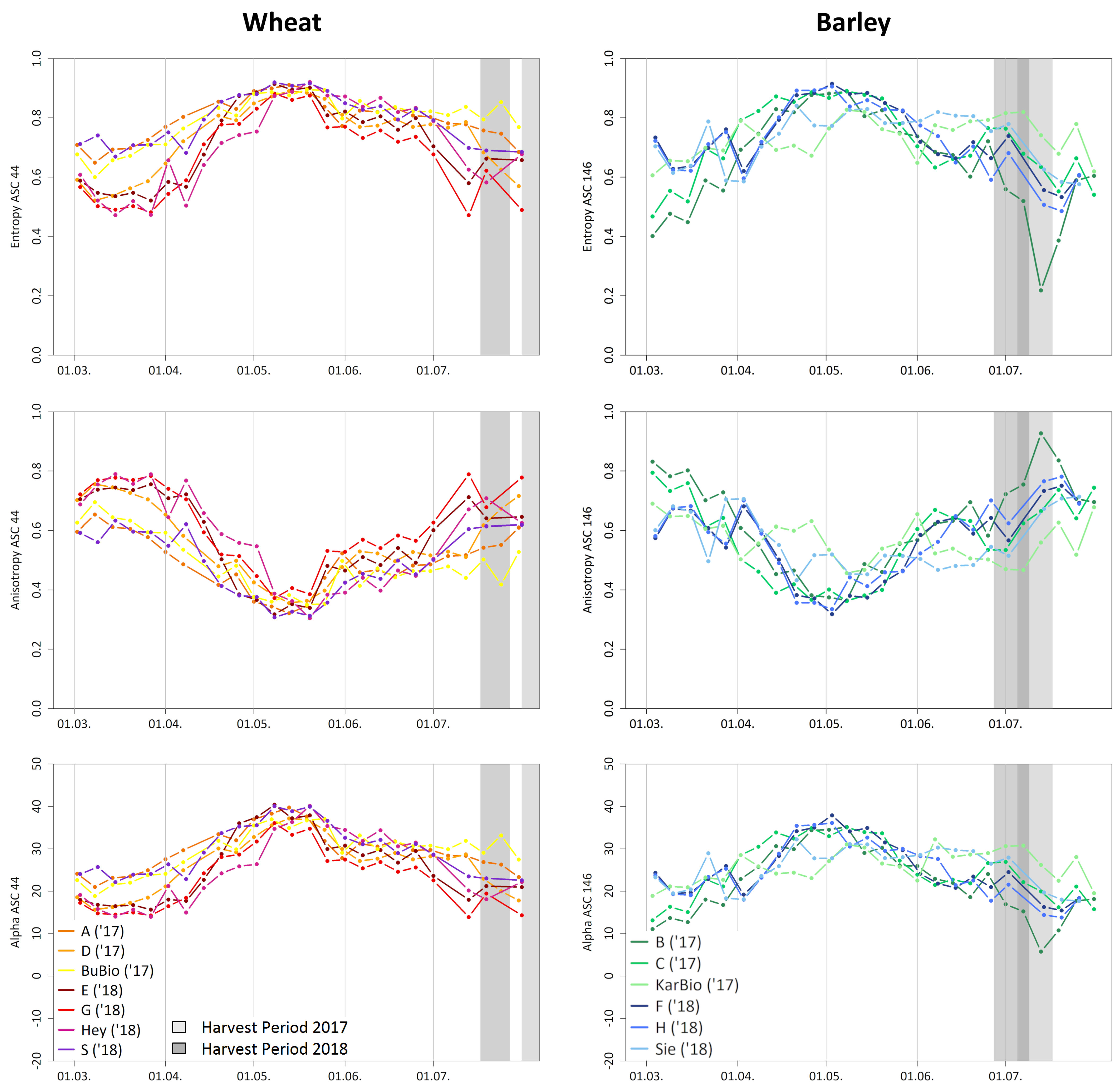
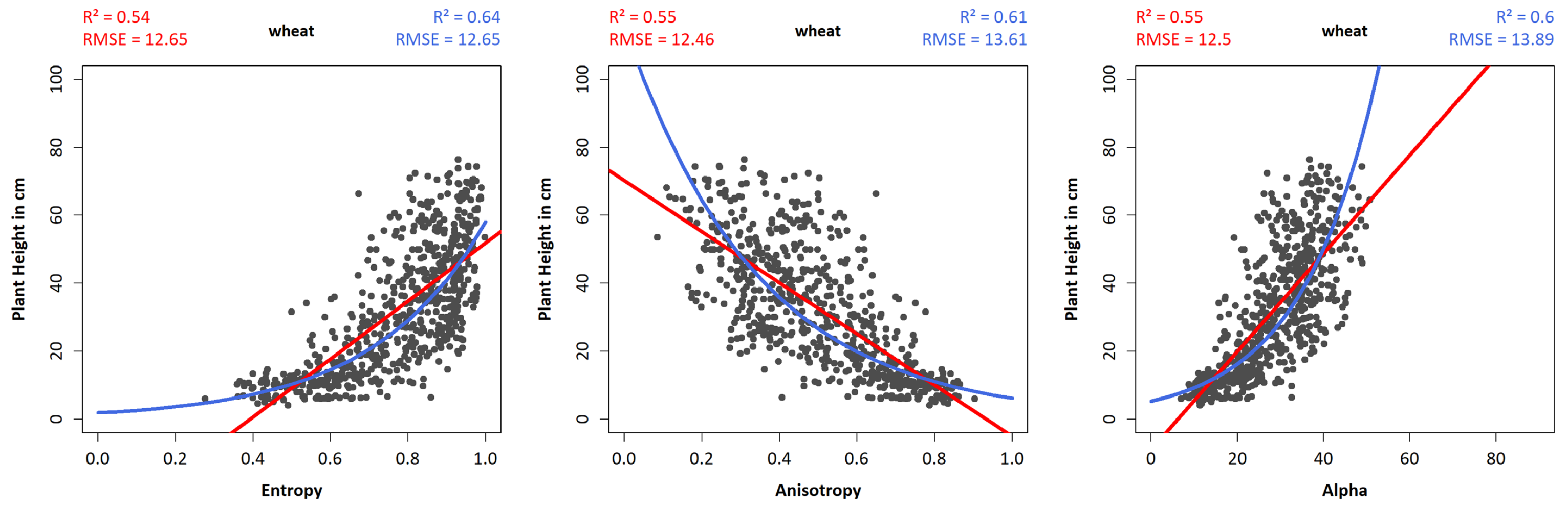
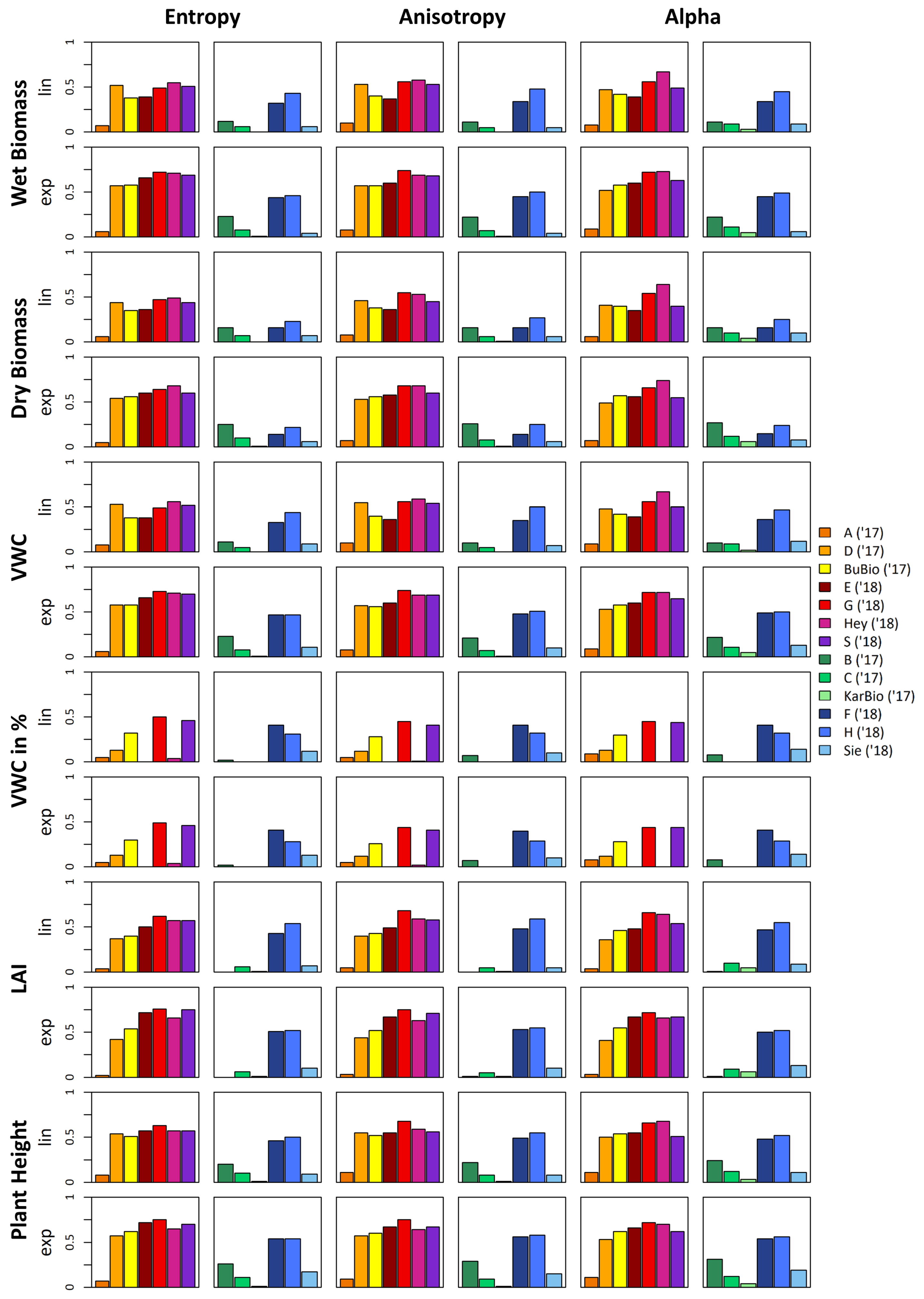
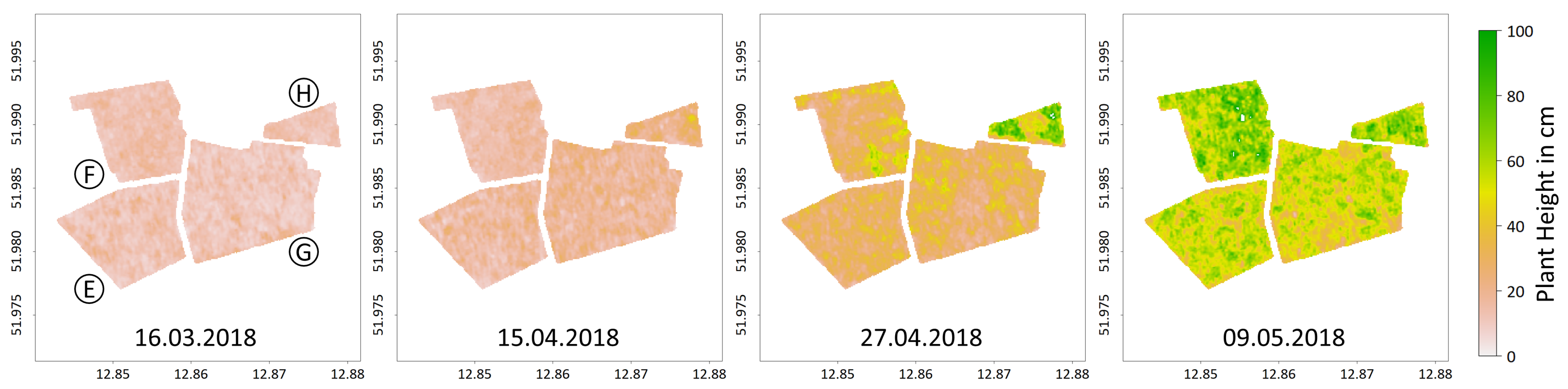
Table 1.
Selected features of the Sentinel-1 data.
| Sentinel-1 | |
|---|---|
| Antenna | C-Band (5.405 GHz) |
| Mode | Interferometric Wide Swath (IW) |
| Swath | 250 km |
| Range Spacing | 2.33 m |
| Azimuth Spacing | 13.89 m |
| Polarization | VV, VH |
| Incidence Angles | 36°–46° |
| Revisit Frequency | 6 days |
| Pass-Orbit Settings | ASC 44, ASC 146 |
| DESC 95, DESC 168 |
Table 2.
Crop parameters obtained during field campaigns 2017 and 2018.
| Crop Parameter (Field) | Unit | Method |
|---|---|---|
| Phenology | Phenological growth stage on the BBCH scale [48] | |
| Plant Height | cm | Average height of ca. 10 plants, measured by the folding rule |
| Number of Leaves | Average number of green leaves of ca. 10 plants | |
| Row Distance | cm | Row distance of crops, stable during vegetation period |
| Crop Coverage | % | Estimated percentage of ground surface covered by crops |
| Chlorophyll Content | μg/cm2 | Average chlorophyll content of 10 leaves of several plants, measured by SPAD device (2017) and DUALEX (2018) |
| Leaf Area Index (LAI) | m2/m2 | Green leaf area per unit ground surface area, average of ca. 10 measurements with SunScan LAImeter |
| Wet Biomass | g/m2 | Weight of fresh plants, destructive sampling of plants in five 1 m rows |
| Crop Parameter (Lab) | ||
| Dry Biomass | g/m2 | Weight of oven-dried plants (at 105 °C until constant weight) |
| Vegetation Water Content (VWC) | g/m2 | Weight difference between wet and dry biomass |
| Relative Vegetation Water Content | % | Weight difference between wet and dry biomass divided by wet biomass |
Table 3.
R2 values of the regression between crop and dual-polarimetric parameters per crop type for all fields: values in parentheses are not significant (p > 0.01). The darker the shade of green, the higher the R2 value.
Table 3.
R2 values of the regression between crop and dual-polarimetric parameters per crop type for all fields: values in parentheses are not significant (p > 0.01). The darker the shade of green, the higher the R2 value.
| ASC146 | Entropy | Anisotropy | Alpha | ||||
|---|---|---|---|---|---|---|---|
| Wheat | Barley | Wheat | Barley | Wheat | Barley | ||
| Wet Biomass | lin | 0.22 | 0.05 | 0.19 | 0.04 | 0.17 | 0.08 |
| exp | 0.41 | 0.08 | 0.35 | 0.07 | 0.34 | 0.11 | |
| Dry Biomass | lin | 0.08 | (0) | 0.06 | (0) | 0.05 | 0.01 |
| exp | 0.29 | 0.02 | 0.24 | 0.02 | 0.23 | 0.04 | |
| VWC | lin | 0.26 | 0.06 | 0.24 | 0.05 | 0.22 | 0.08 |
| exp | 0.46 | 0.12 | 0.4 | 0.11 | 0.39 | 0.16 | |
| VWC in % | lin | 0.04 | 0.07 | 0.05 | 0.07 | 0.05 | 0.06 |
| exp | 0.04 | 0.07 | 0.05 | 0.06 | 0.05 | 0.06 | |
| LAI | lin | 0.3 | 0.04 | 0.28 | 0.03 | 0.26 | 0.07 |
| exp | 0.46 | 0.09 | 0.4 | 0.08 | 0.39 | 0.12 | |
| Plant Height | lin | 0.26 | 0.04 | 0.22 | 0.03 | 0.2 | 0.06 |
| exp | 0.4 | 0.08 | 0.33 | 0.07 | 0.33 | 0.1 | |
Table 4.
R2 values of the regression between crop and dual-polarimetric parameters per crop type for all fields in BBCH stages 21–49. The darker the shade of green, the higher the R2 value.
Table 4.
R2 values of the regression between crop and dual-polarimetric parameters per crop type for all fields in BBCH stages 21–49. The darker the shade of green, the higher the R2 value.
| ASC146 BBCH 21–49 | Entropy | Anisotropy | Alpha | ||||
|---|---|---|---|---|---|---|---|
| Wheat | Barley | Wheat | Barley | Wheat | Barley | ||
| Wet Biomass | lin | 0.4 | 0.09 | 0.43 | 0.09 | 0.42 | 0.13 |
| exp | 0.56 | 0.12 | 0.54 | 0.12 | 0.54 | 0.16 | |
| Dry Biomass | lin | 0.37 | 0.09 | 0.4 | 0.09 | 0.4 | 0.13 |
| exp | 0.52 | 0.1 | 0.52 | 0.1 | 0.52 | 0.13 | |
| VWC | lin | 0.4 | 0.09 | 0.43 | 0.09 | 0.42 | 0.13 |
| exp | 0.56 | 0.16 | 0.54 | 0.16 | 0.53 | 0.2 | |
| VWC in % | lin | 0.24 | 0.12 | 0.2 | 0.11 | 0.2 | 0.13 |
| exp | 0.24 | 0.11 | 0.2 | 0.1 | 0.2 | 0.12 | |
| LAI | lin | 0.42 | 0.1 | 0.44 | 0.09 | 0.43 | 0.14 |
| exp | 0.57 | 0.18 | 0.53 | 0.17 | 0.53 | 0.21 | |
| Plant Height | lin | 0.54 | 0.21 | 0.55 | 0.22 | 0.55 | 0.25 |
| exp | 0.64 | 0.26 | 0.61 | 0.25 | 0.6 | 0.29 | |
Table 5.
R2 values of the regression between crop parameters and backscatter and dual-polarimetric parameters for all wheat fields in BBCH stages 21–49: values in parentheses are not significant (p > 0.01). The parameters of values with asterisk contribute to the multiple regression model. The darker the shade of green, the higher the R2 value.
| ASC146 Wheat BBCH 21–49 | VH | VV | VH/VV | Entropy | Anisotropy | Alpha | Multiple | |
|---|---|---|---|---|---|---|---|---|
| Wet Biomass | lin | 0.22 * | 0.69 * | 0.46 | 0.4 | 0.43 | 0.42 * | 0.7 |
| exp | 0.06 * | 0.6 * | 0.61 | 0.56 * | 0.54 | 0.54 * | 0.68 | |
| Dry Biomass | lin | 0.23 | 0.69 * | 0.44 | 0.37 | 0.4 | 0.4 * | 0.69 |
| exp | 0.09 * | 0.65 * | 0.6 | 0.52 * | 0.52 | 0.52 | 0.7 | |
| VWC | lin | 0.22 * | 0.68 * | 0.45 | 0.4 | 0.42 | 0.42 * | 0.69 |
| exp | 0.05 * | 0.57 * | 0.6 | 0.56 * | 0.54 | 0.53 * | 0.67 | |
| VWC in % | lin | (0.01) * | 0.09 * | 0.21 | 0.24 * | 0.2 | 0.2 * | 0.26 |
| exp | (0.01) * | 0.09 * | 0.2 | 0.23 * | 0.2 | 0.2 * | 0.25 | |
| LAI | lin | 0.19 | 0.65 * | 0.46 | 0.42 | 0.44 | 0.43 * | 0.67 |
| exp | 0.03 * | 0.52 * | 0.58 | 0.57 * | 0.53 | 0.53 * | 0.64 | |
| Plant Height | lin | 0.12 * | 0.71 * | 0.61 | 0.54 | 0.55 | 0.55 * | 0.75 |
| exp | 0.05 * | 0.65 * | 0.69 | 0.64 * | 0.61 | 0.6 * | 0.76 | |
Table 6.
R2 values of the regression between crop parameters and backscatter and dual-polarimetric parameters for all barley fields in BBCH stages 21–49: the parameters of values with asterisk contribute to the multiple regression model. The darker the shade of green, the higher the R2 value.
Table 6.
R2 values of the regression between crop parameters and backscatter and dual-polarimetric parameters for all barley fields in BBCH stages 21–49: the parameters of values with asterisk contribute to the multiple regression model. The darker the shade of green, the higher the R2 value.
| ASC146 Barley BBCH 21–49 | VH | VV | VH/VV | Entropy | Anisotropy | Alpha | Multiple | |
|---|---|---|---|---|---|---|---|---|
| Wet Biomass | lin | 0.36 * | 0.38 * | 0.11 | 0.09 * | 0.09 | 0.12 * | 0.44 |
| exp | 0.2 * | 0.3 * | 0.14 | 0.12 | 0.12 | 0.16 * | 0.32 | |
| Dry Biomass | lin | 0.32 * | 0.35 * | 0.11 | 0.09 * | 0.09 | 0.13 * | 0.41 |
| exp | 0.14 * | 0.22 * | 0.1 | 0.1 * | 0.1 | 0.13 * | 0.24 | |
| VWC | lin | 0.38 * | 0.41 * | 0.12 | 0.09 * | 0.09 | 0.13 * | 0.47 |
| exp | 0.28 * | 0.42 * | 0.2 | 0.16 * | 0.16 | 0.2 * | 0.44 | |
| VWC in % | lin | 0.2 | 0.33 * | 0.17 | 0.12 | 0.11 | 0.13 | 0.33 |
| exp | 0.19 | 0.32 * | 0.17 | 0.11 | 0.1 | 0.12 | 0.32 | |
| LAI | lin | 0.34 * | 0.4 * | 0.14 | 0.1 * | 0.09 | 0.14 * | 0.45 |
| exp | 0.27 * | 0.46 * | 0.24 | 0.18 | 0.17 | 0.21 | 0.46 | |
| Plant Height | lin | 0.43 * | 0.62 * | 0.28 | 0.21 * | 0.22 | 0.25 * | 0.64 |
| exp | 0.39 * | 0.64 * | 0.33 | 0.26 | 0.26 | 0.29 * | 0.65 | |
Publisher’s Note: MDPI stays neutral with regard to jurisdictional claims in published maps and institutional affiliations. |
© 2021 by the authors. Licensee MDPI, Basel, Switzerland. This article is an open access article distributed under the terms and conditions of the Creative Commons Attribution (CC BY) license (http://creativecommons.org/licenses/by/4.0/).
Share and Cite
MDPI and ACS Style
Harfenmeister, K.; Itzerott, S.; Weltzien, C.; Spengler, D. Agricultural Monitoring Using Polarimetric Decomposition Parameters of Sentinel-1 Data. Remote Sens. 2021, 13, 575. https://0-doi-org.brum.beds.ac.uk/10.3390/rs13040575
AMA Style
Harfenmeister K, Itzerott S, Weltzien C, Spengler D. Agricultural Monitoring Using Polarimetric Decomposition Parameters of Sentinel-1 Data. Remote Sensing. 2021; 13(4):575. https://0-doi-org.brum.beds.ac.uk/10.3390/rs13040575
Chicago/Turabian StyleHarfenmeister, Katharina, Sibylle Itzerott, Cornelia Weltzien, and Daniel Spengler. 2021. "Agricultural Monitoring Using Polarimetric Decomposition Parameters of Sentinel-1 Data" Remote Sensing 13, no. 4: 575. https://0-doi-org.brum.beds.ac.uk/10.3390/rs13040575
Note that from the first issue of 2016, this journal uses article numbers instead of page numbers. See further details here.