Article

Machine Learning Classification of Mediterranean Forest Habitats in Google Earth Engine Based on Seasonal Sentinel-2 Time-Series and Input Image Composition Optimisation

by
Salvatore Praticò
1,
Francesco Solano
2,*,
Salvatore Di Fazio
1 and
Giuseppe Modica
1
1
Dipartimento di Agraria, Università degli Studi Mediterranea di Reggio Calabria, Località Feodi Vito, I-89122 Reggio Calabria, Italy
2
Department of Agriculture and Forest Sciences (DAFNE), University of Tuscia, via S. Camillo de Lellis, 01100 Viterbo, Italy
*
Author to whom correspondence should be addressed.
Submission received: 23 December 2020 / Revised: 3 February 2021 / Accepted: 4 February 2021 / Published: 7 February 2021

Abstract

:
The sustainable management of natural heritage is presently considered a global strategic issue. Owing to the ever-growing availability of free data and software, remote sensing (RS) techniques have been primarily used to map, analyse, and monitor natural resources for conservation purposes. The need to adopt multi-scale and multi-temporal approaches to detect different phenological aspects of different vegetation types and species has also emerged. The time-series composite image approach allows for capturing much of the spectral variability, but presents some criticalities (e.g., time-consuming research, downloading data, and the required storage space). To overcome these issues, the Google Earth engine (GEE) has been proposed, a free cloud-based computational platform that allows users to access and process remotely sensed data at petabyte scales. The application was tested in a natural protected area in Calabria (South Italy), which is particularly representative of the Mediterranean mountain forest environment. In the research, random forest (RF), support vector machine (SVM), and classification and regression tree (CART) algorithms were used to perform supervised pixel-based classification based on the use of Sentinel-2 images. A process to select the best input image (seasonal composition strategies, statistical operators, band composition, and derived vegetation indices (VIs) information) for classification was implemented. A set of accuracy indicators, including overall accuracy (OA) and multi-class F-score (Fm), were computed to assess the results of the different classifications. GEE proved to be a reliable and powerful tool for the classification process. The best results (OA = 0.88 and Fm = 0.88) were achieved using RF with the summer image composite, adding three VIs (NDVI, EVI, and NBR) to the Sentinel-2 bands. SVM and RF produced OAs of 0.83 and 0.80, respectively.

Graphical Abstract

1. Introduction

The contemporary management and conservation of natural heritage have assumed strategic importance globally. In the European Union, a key role is played by the Natura 2000 network, which is a network of high-natural-value sites to be protected, set up in the framework of two different, but integrated, European directives (79/409/EEC—Birds Directive and 92/43/EEC—Habitat Directive). In this context, to ensure the achievement of the related conservation aims, a repeatable method is needed to monitor the changes in habitats and species occurring over time [1]. Moreover, each European Member State must report, every six years, the status of protected habitats and species that fall within its borders [2]. Accordingly, knowledge of the spatial pattern of typical species is fundamental for habitat monitoring issues. Forests play a major role in nature conservation. Their specific monitoring is relevant to the detection of ongoing degradation processes, as is the case of many Mediterranean forests [3], and addressing future sustainable strategies for landscape planning to strengthen the positive trends and hinder the negative ones [4].
Land-use and land-cover (LU/LC) classification represents pivotal information to understand human–environment relationships [5,6,7]. For mapping and conservation-related issues, remote sensing (RS) techniques and geographic information systems (GIS) have been widely used, in part due to the ever-growing availability of free data and software [8,9,10,11,12,13]. At present, many researchers take advantage of high-resolution satellite imagery, making landscape analysis more precise and, thus, improving the resulting accuracy [14]. RS satellite data are a useful source for LU/LC classification and change detection, offering some advantages and enabling landscape observation, mapping, assessment, and monitoring, for either general or specific purposes [15,16,17,18,19,20]. RS allows for rapid map production, especially for hard-to-reach regions [21]. Moderate-resolution image spectroradiometer (MODIS) data have been used to estimate different vegetation characteristics, such as leaf area index, biomass, and productivity [22,23,24]. However, a finer spatial resolution than that provided by MODIS is often required [25]. Free data from the Landsat (https://www.usgs.gov/core-science-systems/nli/landsat) and Sentinel missions (https://sentinel.esa.int/web/sentinel/home) have been used to monitor LC changes at different scales and in different environments [26,27,28]. Landsat data and RS techniques have been used to monitor natural habitats in Germany [29]. Chetan et al. [30] performed an analysis of the changes in the most common natural habitat types of Romanian mountains using Landsat time-series and an object-based classification approach. Bock et al. [31] performed a comparison between pixel- and object-based classification approaches to monitor some Natura 2000 areas of Germany and the United Kingdom using Landsat free satellite data. Wang and Xu [32] compared the performance of different RS techniques in detecting landscape changes to assess hurricane damage to forests in the United States of America. Free satellite data and landscape metrics have been used by Pôças et al. [33] to analyse mountain landscape changes in North Portugal. Pastick et al. [34] used Landsat-8 OLI and Sentinel-2 MSI jointly to characterise seasonal vegetation index (VI) signatures in a drylands environment.
The classical RS spectral approach in LC mapping and monitoring is not easy to perform in mountain forests, where the spectral similarity between different species might be misleading. Moreover, mountainous areas are often characterised by frequent cloud coverage, which may affect the results of single-image LC discrimination. To achieve accurate scene classification, a multi-scale and multi-temporal approach is needed, in order to detect the different phenological aspects that characterise different vegetation types and species [35,36]. This type of approach also solves the problem of the presence of clouds [6]. Variation in spectral vegetation indices (VIs) has been linked to seasonal phenological changes due to different photosynthetically active leaf area responses, highlighting seasonal vegetation variation due to growth–senescence alternation [37,38]. Information related to phenology is crucial for ecologists and land managers, because they can obtain essential insights about species composition, distribution patterns, and the vigour of vegetation and forest habitats in general [39,40].
The time-series composite image approach allows for capturing much of the variability in the spectra of different LC types, as widely demonstrated in such complex environments as mountain forests [6,41,42,43,44,45]. The analysis of phenological differences during a selected time period (e.g., one year or consecutive years) can help to discriminate between different forest types [46,47,48]. RS geospatial big data [49] can reflect the dynamic state of the earth’s surface, which undergoes continuous change. Such multi-temporal big data approaches present some critical aspects, basically due to the time-consuming activity of satellite-data searching and downloading, as well as the huge storage space needed for the associated petabytes of RS data. Moreover, powerful computational processing capacities are required to manage all data and to run the different algorithms.
To address the aforementioned issues, a novel approach must be used. There are two different common system architecture solutions: cluster-based high-performance computing systems and cloud-based computation platforms [50]. The former involves the co-operation of several computers with a single-system image, allowing for strong computational capability but suffering high load and processing massive volumes of data [14]. On the other hand, cloud-based platforms—that is, virtualising supercomputer infrastructures—offer a more user-friendly approach.
The Google Earth engine (GEE; https://earthengine.google.com) [51] is a free cloud-based computational platform that uses Google’s cloud and JavaScript-based language to access and process petabyte scales of remotely sensed data on a global scale. GEE takes advantage of Google’s computational infrastructure to reduce operational time and provide a repository for script storing and sharing, allowing for broad collaboration between different users with minimal cost and equipment. The GEE data catalogue allows access to multiple satellite data and satellite-derived products [52].
Moreover, GEE offers different image collecting, analysis, processing, classification, and export packages, ensuring that users no longer have to depend solely on commercial software [14,52,53]. To date, GEE has been widely used for different mapping purposes; primarily to exploit its massive catalogue of images to capture time-series data or derive useful information to analyse phenomena over a long period. The capabilities of GEE, jointly with external software and applications, have been widely explored using different data and algorithms for a wide range of applications, such as forest mapping [26,54,55], LU/LC classification [56,57], fire severity analysis [58], forest disturbance mapping [59], forest defoliation assessment [60], surface water detection [61], mine mapping [62], snow [63] and shoreline detection [64], urban and rural settlement mapping [65,66], and species habitat monitoring [67].
This paper proposes a novel approach which is entirely developed in the GEE environment, exploiting its full potential to test different combinations of variables and obtain solid data collection to improve each classification step. Moreover, this approach has made it possible to exploit the strengths of both an unsupervised and supervised classification to optimise the acquisition of input data and then achieve the highest levels of accuracy.
The novelty of this research relies upon the proposed workflow for analysing different image and variable composites (i.e., seasonal image collections, reflectance bands, and VIs) to improve Mediterranean mountainous forest habitat classification accuracy. Moreover, the in-depth investigation of these data and their combination enabled us to optimise training and validation points selection, which is a delicate step in the classification process.
Furthermore, we aimed to make the analysis, classification, and mapping processes accessible to different users with different backgrounds and software and hardware availabilities. Therefore, it was crucial to test GEE’s responses, in order to carry out the entire work process without using third-party applications.
Furthermore, all scripts can be shared, edited, and updated for rapid application, in order to support decision-making in planning and monitoring activities.
The research reported in this paper was conceived with three main objectives:
  • To test the potential of the GEE platform and Sentinel-2 data to classify forest habitat in a protected natural national park representative of the Mediterranean region, which includes remarkable Natura 2000 sites, performing the whole process inside the code editor environment of GEE;
  • To test how different variables and their combinations, all available in GEE, can improve the classification performance (e.g., combinations of input images, bands, reflectance indices, and so on);
  • To compare and assess the performance of different machine-learning classification algorithms, in terms of the obtained classification accuracy.
Our goal was to define a method which, although tested in a specific region, might be adapted and applied in a broader context concerning the same classification issue, using similar data types and for similar Mediterranean Natura 2000 forest habitats.

2. Materials and Methods
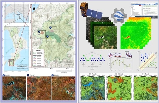
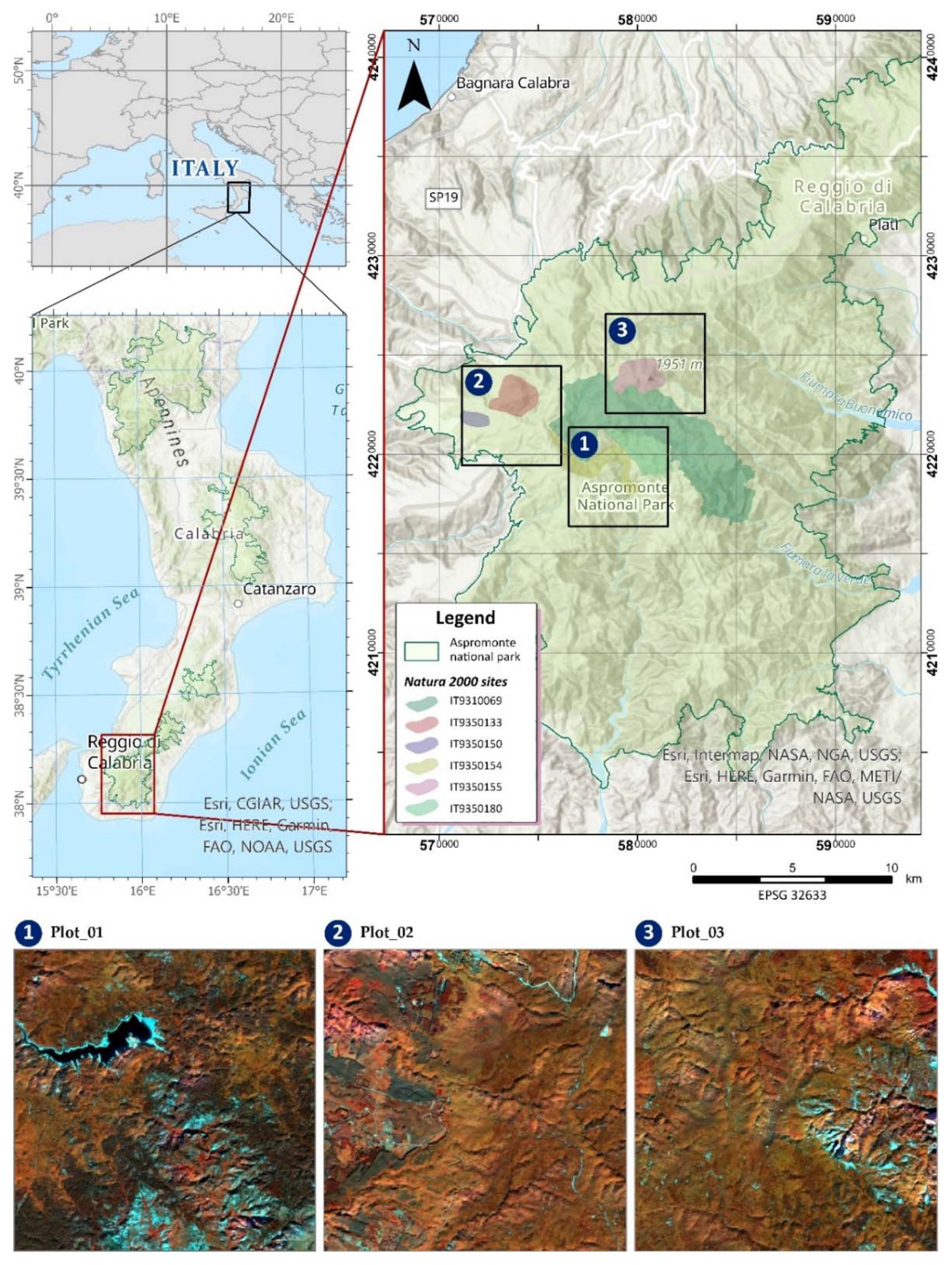
Our proposed method, overviewed in Figure 1 and applied in an Italian mountainous protected area, was based entirely on the use of the GEE cloud platform environment.
Starting from the available images in the GEE catalogue, we built a consistent time-series. We tested how the use of different compositions of images, grouped according to their seasonality, together with different combinations of spectral bands and VIs, affected the classification result, leading to identification of the best input image that provided the highest accuracy. Finally, this image was used to test three different classifiers, in order to detect which of them provided the best result, in terms of classification accuracy.
Our proposed method can be summarised as follows: image pre-processing, including image selection, filtering, and time-series building; image processing (derivation of seasonal information, image reduction); classification (training and validation points acquisition, best input image selection, supervised machine learning algorithms and parameters optimisation); accuracy assessment and comparison; and mapping.

2.1. Study Area

The study area where the method was applied is part of the natural Aspromonte National Park, in the Calabria region (Southern Italy; see Figure 2).
This natural park was established in 1994 and had a total surface of 65,647.46 ha (www.parcoaspromonte.gov.it—last accessed on 5 November 2020).
Aspromonte National Park is located in the very south of Calabria, and presents altitudes ranging from 100 m a.s.l to 1956 m a.s.l., with the highest peak corresponding to Mt. Montalto. Calabria is located in the extreme south of the Italian peninsula, covering about 15,000 km2, and presents an elongated shape, extending north to south and separating the Ionian Sea from the Tyrrhenian Sea. Calabria lies in the centre of the Mediterranean basin, and shows a typical, although diversified, Mediterranean climate [67]. The Apennine Mountains run along the central part of the region, marking climatic differences between the Ionian and Tyrrhenian sides [68].
This climate diversity is mirrored by an analogous diversity in vegetation composition and distribution [69], playing an essential role in defining and maintaining a natural habitat network [70]. This is why we decided to locate the study area in the Aspromonte National Park, where considerable forest biodiversity within a relatively small area can be observed, thus making LU/LC classification particularly challenging. Aspromonte is characterised by a gradient of natural vegetation, following the altitudinal belts from the Meso-Mediterranean Holm oak forests (Quercus ilex L.) and thermophilous oak forests (Quercus frainetto Ten., Quercus pubescens s.l.) to mountain black pine forests (Pinus nigra subsp. Calabrica Loud.) and beech forests (Fagus sylvatica L.) with fir (Abies alba Mill.). This vegetation complex contains many endemic (Calabrian) and sub-endemic (Calabrian–Sicilian) plant species [71].
In Aspromonte, pure and mixed beech stands can also be found, including the occurrence of essential priority habitats for natural conservation in Europe (9210* Apennine beech forests with Taxus and Ilex and 9220* Apennine beech forests with Abies alba and beech forests with Abies nebrodensis), along with Calabrian pine afforestations and pure Apennine silver fir (Abies alba subsp. Apennina Brullo, Scelsi, & Spamp.) woodlands, especially on steep slopes [69]. Finally, at the lower altitudes, chestnut woods (Castanea sativa Mill.) are also planted in the supra-Mediterranean belt or the one below, which are usually managed as coppice systems. To include all these different LU/LC classes, three different square plots, covering a total surface of 75 km2 (25 km2 each), were defined within the Aspromonte National Park (Figure 2). Moreover, the following Natura 2000 sites fell into the three plots: (i) IT9310069 “Parco Nazionale della Calabria”; (ii) IT9350133 “Monte Basilicò—Torrente Listì”; (iii) IT9350150 “Contrada Gornelle”; (iv) IT9350154 “Torrente Menta”; (v) IT9350155 “Montalto”; and (vi) IT9350180 “Contrada scala”. These sites hosted several relevant forest habitats, such as Apennine beech forests with Taxus and Ilex (code 9210*), Apennine beech forests with Abies alba and beech forests with Abies nebrodensis (code 9220*), Castanea sativa woods (code 9260), Southern Apennine Abies alba forests (code 9510*), and (Sub-)Mediterranean pine forests with endemic black pines (code 9530*).

2.2. Image Pre-Processing

2.2.1. Satellite Data Selection

According to Chaves et al. [18], we used Sentinel-2 imagery, because its bands are considered more suitable for vegetation analysis, thanks to its finer spatial resolution compared to other satellite images and its wavelength sensitivity to chlorophyll content and phenological states [72], making the VIs more accurate for LU/LC discrimination [73].
The payload carried on Sentinel-2 is a multispectral sensor with 13 bands at different ground resolutions (Table 1).
Sentinel-2 data are available in two different levels, based on the atmospherical correction status of the images: Level 1C for top-of-atmosphere (TOA) images, and Level 2A for bottom-of-atmosphere (BOA) reflectance. The former need to be atmospherically corrected, in order to obtain useful reflectance values. This correction cannot be carried out in the GEE JavaScript-based environment, but requires third-party applications or Python API [74,75,76]. To adhere to the research objectives, we used level 2A images, which are already atmospherically corrected.
In the GEE code editor environment, we imported Sentinel-2 level 2A images as an image collection (i.e., a set of Google Earth engine images).

2.2.2. Image Filtering and Time-Series Extraction

To reduce the image collection step, a filtering process was needed. In this work, we filtered the image collection using three variables: covered location, time interval, and cloud percentage. The location of the images was given by the boundaries of the three square plots under study that we imported in GEE environment. The time period was fixed, starting from 28 March 2017 (the first Sentinel-2 BOA available image in GEE) to 31 July 2020, thus covering more than three consecutive years. Finally, we used the cloudy pixel percentage value, stored as metadata for each image, to select and extract only those images with a cloud cover less than 10% in the study area.

2.3. Image Processing

2.3.1. Vegetation Indices

Time-series can be used to extract the seasonal variability of each pixel, using the values of several VIs as indicators [42,77]. The link between VIs and vegetation phenological variability is more robust than that of single bands [78]. Computing different VIs for each image of a time-series can be a time-consuming activity. The GEE JavaScript-based code editor environment allows for the straightforward and simultaneous calculation of VIs for each time-series image.
All computed indices can be added as a separate band for each image. Six VIs, listed in Table 2, were taken into account in this work.
The first index was the normalised difference vegetation index (NDVI) [79], based on the normalised ratio of near infrared (NIR) and red bands. This is a well-known and widely used VI, which allows for the identification of photosynthesising vegetation by investigating the bands of higher absorption and chlorophyll reflectance. The NDVI can assume values between −1 and 1.
The green normalised difference vegetation index (GNDVI) [80] has been developed to estimate leaf chlorophyll concentration, and uses the green band instead of the red band in the NDVI formula.
The enhanced vegetation index (EVI) [81] involves the NIR, red, and blue bands. It has been developed to achieve better sensitivity in high biomass regions and be more responsive to different species’ canopy structural variation by decoupling the canopy background.
The normalised ratio between NIR and short wave infrared (SWIR) bands was taken into account to compute two different indices: the normalised difference infrared index (NDII) [82] and normalised burn ratio (NBR) [83]. Both indices consider the shortwave-infrared region, a portion of the spectrum which is sensitive to leaf water content. In general, SWIR reflectance decreases when leaf water content increases [84]. The NDII and NBR formulae differ in the SWIR wavelength investigated [85]. The former investigates the region between 1550 nm and 1750 nm (Sentinel-2 B11), while the latter considers the region between 2050 nm and 2450 nm (Sentinel-2 B12).

2.3.2. Image Reduction

All collected images were split into sub-time-series by month of acquisition and grouped to represent different seasonal periods. In this way, we obtained: (i) a winter set of images that highlights the no-leaf status of deciduous species, composed of images acquired in December-March (W_IC); (ii) a late spring–early summer set from April-June (Sp_IC), representing the period of vegetative restart and growth; (iii) a summer set, corresponding to the maximum potential vegetation activity, collected in July-September (Su_IC); and (iv) an autumn set, during the start of the senescence period, highlighted by images from October and November (A_IC), when the leaves of deciduous trees turn to yellow and red colours.
All of the time-series had to be reduced to a single image, containing each selected image’s information, to perform the classification.
To obtain a single image, a process of reduction was needed. Single images of the image collection represented the input.
The output, computed pixel-wise, was a new image for which values of all images provide each pixel value in the collection at a given location. The final value was computed using statistical operations. We used the median, mean, maximum, and minimum values of pixels to perform the reduction.

2.4. Classification

The classification can be performed either by pixel- or object-based approaches. It has been widely demonstrated that object-based approaches can provide more accurate results when using high- and very high-resolution data [86,87,88]. In contrast, when the object’s dimension is smaller than the pixel resolution (e.g., when a single-tree canopy is to be detected in images with 10 m spatial resolution), a pixel-based approach is preferable.
In this study, considering the resolution of the images used to carry out the supervised classification of LC, we adopted a pixel-based approach which, according to Tamiminia et al. [14], is considered as the GEE approach and has been most adopted by the scientific community.
Considering the characteristics of the area and our previous research experiences [89], we chose seven LC classes to perform the classification: water (Wa), bare soil (BS), roads (Ro), chestnut woodland (CW), beech woodland (BW), silver fir woodland (SW), and pine woodland (PW).

2.4.1. Unsupervised Clustering

The first classification step concerned the discrimination between the coniferous and broadleaf forest components, in order to derive homogeneous areas to collect SW and PW class training points in the subsequent process. To this end, an unsupervised classification was performed, in order to highlight potential areas of localisation of these forest types, using W_IC to exploit the leaf-off condition to better distinguish conifers from deciduous broad-leaved woods. Among the various classification approaches, unsupervised image classification methods have the advantage of using the overall spectral content of an image [90], with the essential condition that, in this case, the goal was to grasp the thematic homogeneity represented by conifers. The unsupervised classification was performed in the GEE environment, using the K-means clustering algorithm [91,92,93].
This classifier calculates class means that are evenly distributed in the data space, and then iteratively tries to cluster data, according to their similarity, using minimum spectral distance techniques [94]. Each iteration recalculates means and reclassifies pixels concerning the new means. All pixels are classified to the nearest class using a distance threshold.
In this case, the clustering was based on the Euclidean distance. Once the process was completed, a new layer was obtained, with the homogeneous areas represented only by conifers. The result was validated using ground truth data points.

2.4.2. Determination of Training and Validation Points

To improve the quality of the final classification results, the choice of training and validation points is one of the most critical steps in the whole process [95]. The in-depth investigation of all the available images and the possibility of efficiently combining them to create seasonal ICs enabled us to optimise the selection of training and validation points, thus allowing us to use reference layers that highlighted different forest species behaviours (e.g., winter images allowed for better coniferous detection). The classification method used was pixel-based; therefore, training and validation points represented the defined LC classes to which they belonged, avoiding mixed pixel issues.
For each LC class, a set of 100 points (700 in total) was collected in the GEE map area environment using different reference layers (i.e., unsupervised clustering output, in situ surveys, and different ICs). Each set was formed of 25 training points (25% of the total) and 75 validation points (75% of the total), for each class; thus, with a total number of 175 training points and 525 validation points. All training points were collected through a visual approach, while the validation points were collected, on one hand, using a visual approach justified by a thorough knowledge of the area and, on the other hand, only for the forest LC classes, using several points of known co-ordinates surveyed directly in the field. A total of 50 ground truth points were randomly collected in situ, 20 for the BW class and 10 each for CW, SW, and PW classes. As mentioned previously (see Section 2.4.1), we used the map resulting from the unsupervised clustering, detecting the two main coniferous woodland species existing in the scene, as a reference layer for the collection of coniferous class training points. The winter composite image was used to collect validation points, due to its capacity to highlight the species of interest. For BS and Ro class points, we used the summer composite image as a reference layer for both training and validation points, avoiding the wrong assignment of points caused by a temporary uncovering of the soil due to the regular growth cycles of vegetation. CW and BW class training and validation points were collected using the autumn composite image. In this season, the two broad-leaved species present a different colour, due to the higher concentration of carotenoid and anthocyanin pigments caused by the senescence period [96]. Considering that these two species occupy different altitudinal limits, we added the information provided by the 30 m spatial resolution digital elevation model (DEM) available in GEE. Wa points detection did not need a specific image as a reference and, thus, the Su_IC was used as reference layer for both training and validation points.

2.4.3. Machine Learning Classification Algorithms

The GEE environment integrates several different classifiers. We compared the performance of three of them, chosen according to their wide use and reliability in LC classification [11,14,86,97,98,99,100,101]: random forest (RF), classification and regression tree (CART), and support vector machine (SVM).
RF [102] is a decision method based on using a decision forest consisting of many individual decision trees that operate as an ensemble. Each tree is trained in a different training set from the original one using bootstrap aggregation (namely, bagging) and generating an error estimate, including observations that occur in the original data and not in the bootstrap sample [103].
RF in GEE allows for setting different parameters: the number of decision trees in the forest, the number of variables per split, the minimum leaf population, the bag fraction (i.e., the proportion of training data to be used in the creation of the next tree in the boost), the maximum number of nodes in each tree, and the randomisation seed.
CART [104,105], similar to RF, is a single tree decision classifier. One attribute splits the data into subsets at each node of the tree based on the normalised information gain, resulting in the split’s defining attribute. The attribute with the higher value of normalised information gain is chosen to make the final decision [106]. In GEE, only two parameters can be set: the minimum leaf population and the maximum number of nodes.
SVM [107,108] is a non-parametric supervised classifier based on kernel functions. To train the algorithm, SVM learns the boundary between trainers belonging to different classes, projecting them in a multidimensional space and finding one or more hyperplanes maximising the separation of the training data set between the pre-defined number of classes [109].
In the GEE environment, several parameters can be set: the decision procedure (voting or margin), the Kernel type (linear, polynomial, sigmoid, or radial basis function), and the C parameter (how many samples inside the margin contribute to the overall error). Based on these parameters, others can be set (e.g., Kernel degree, if a polynomial function is chosen).
Different combinations of parameters were tested for each classifier with a trial-and-error approach, reporting and comparing the obtained accuracy.

2.4.4. Choice of the Best Input Image for Classification

As highlighted by Phan et al. [110], the choice of the input image can influence the accuracy of the classification process. Different images lead to different accuracy values at the end of the classification process.
To assess the best achievable accuracy, we exploited GEE’s potential, which allowed us to test several different input images quickly. They were differentiated, according to the different variables composing each of them, such as band number, reflectance regions, VIs, and statistics used to reduce the image collection (e.g., mean, median, minimum, and maximum values of the pixel). A trial-and-error approach was carried out, testing how the use of one variable rather than another, and their possible combinations, might affect the final classification result. To test the effects of different images on the classification, we used the accuracy values and out-of-bag (OOB) error estimates as indicators. OOB is an unbiased estimate of the actual prediction error of RF and other machine learning algorithms.

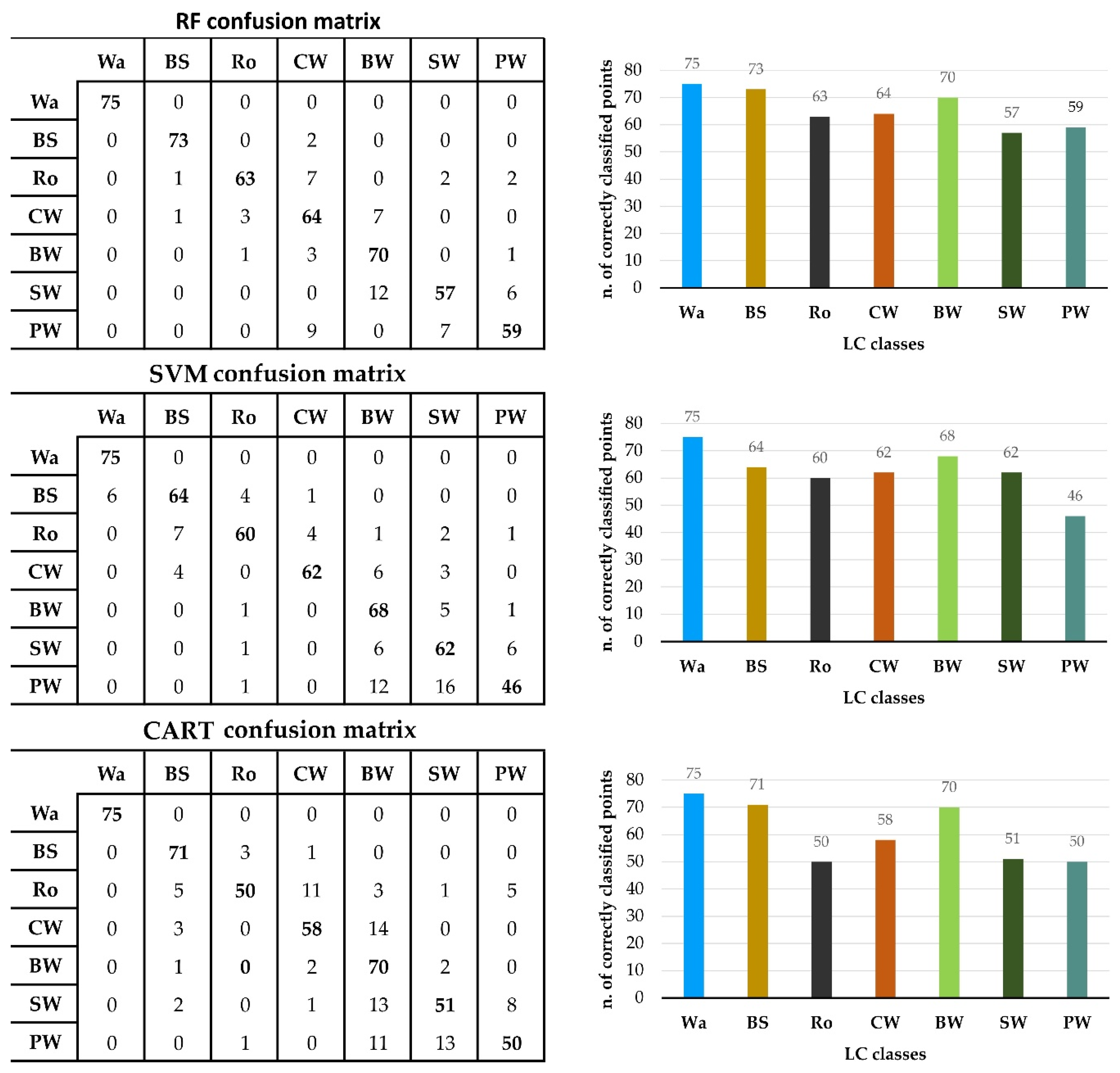
2.5. Accuracy Assessment
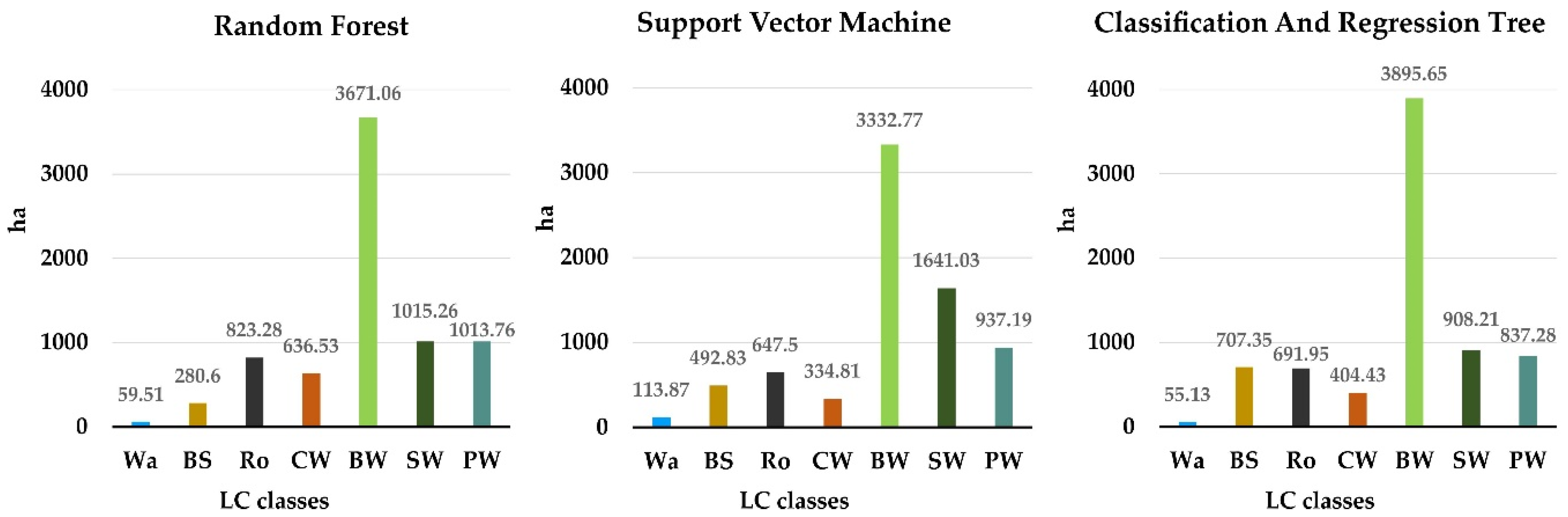
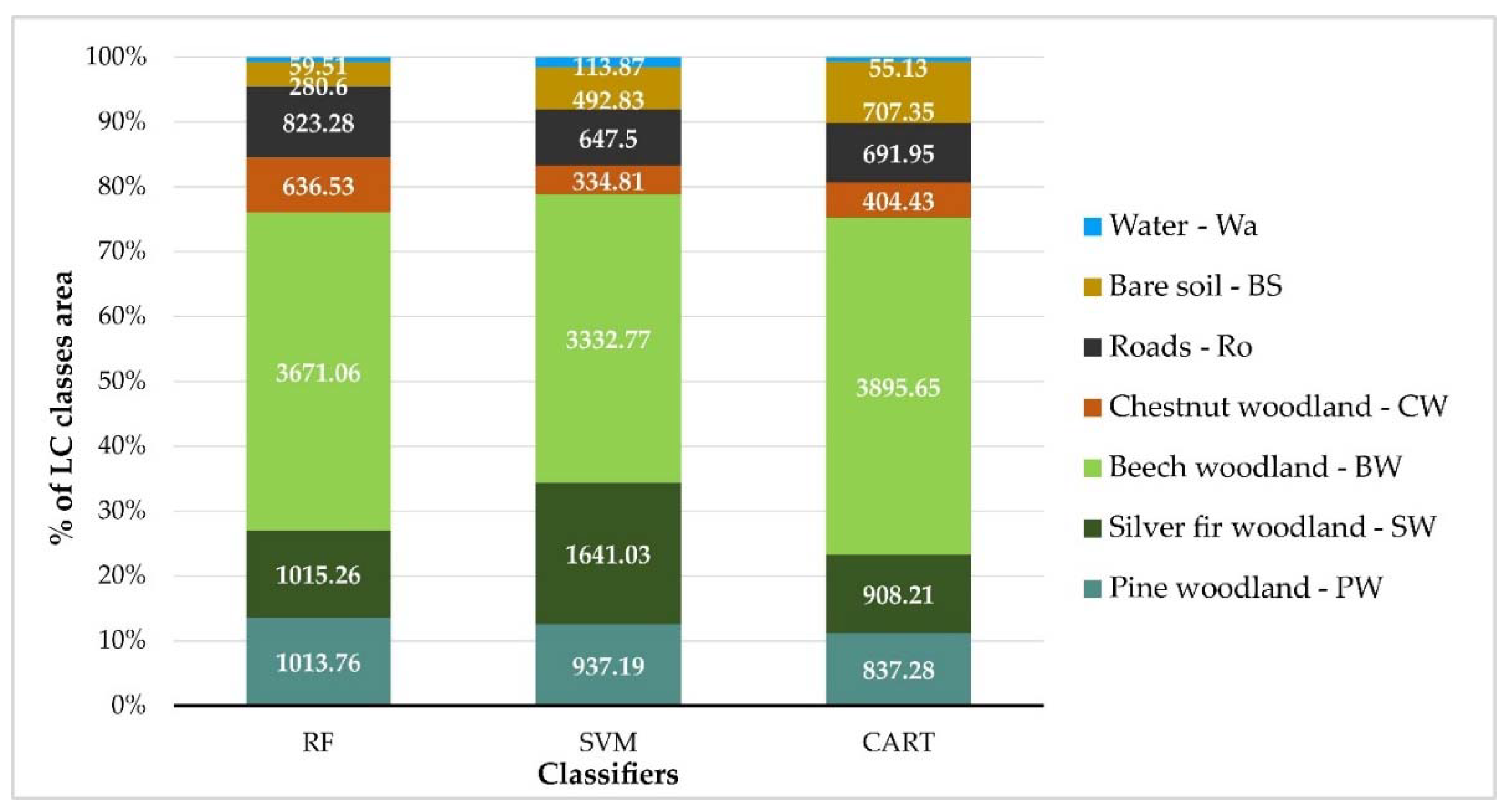
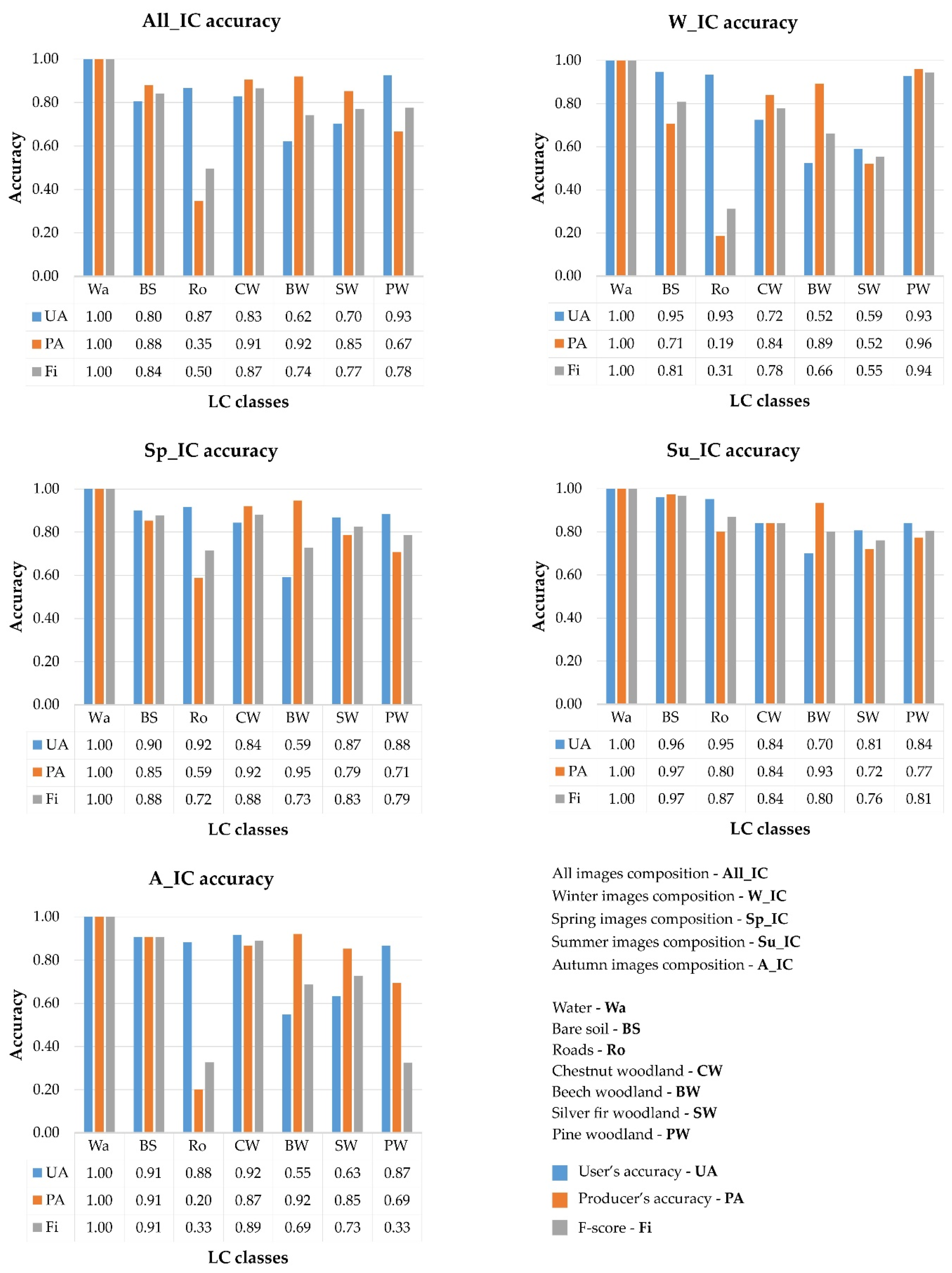
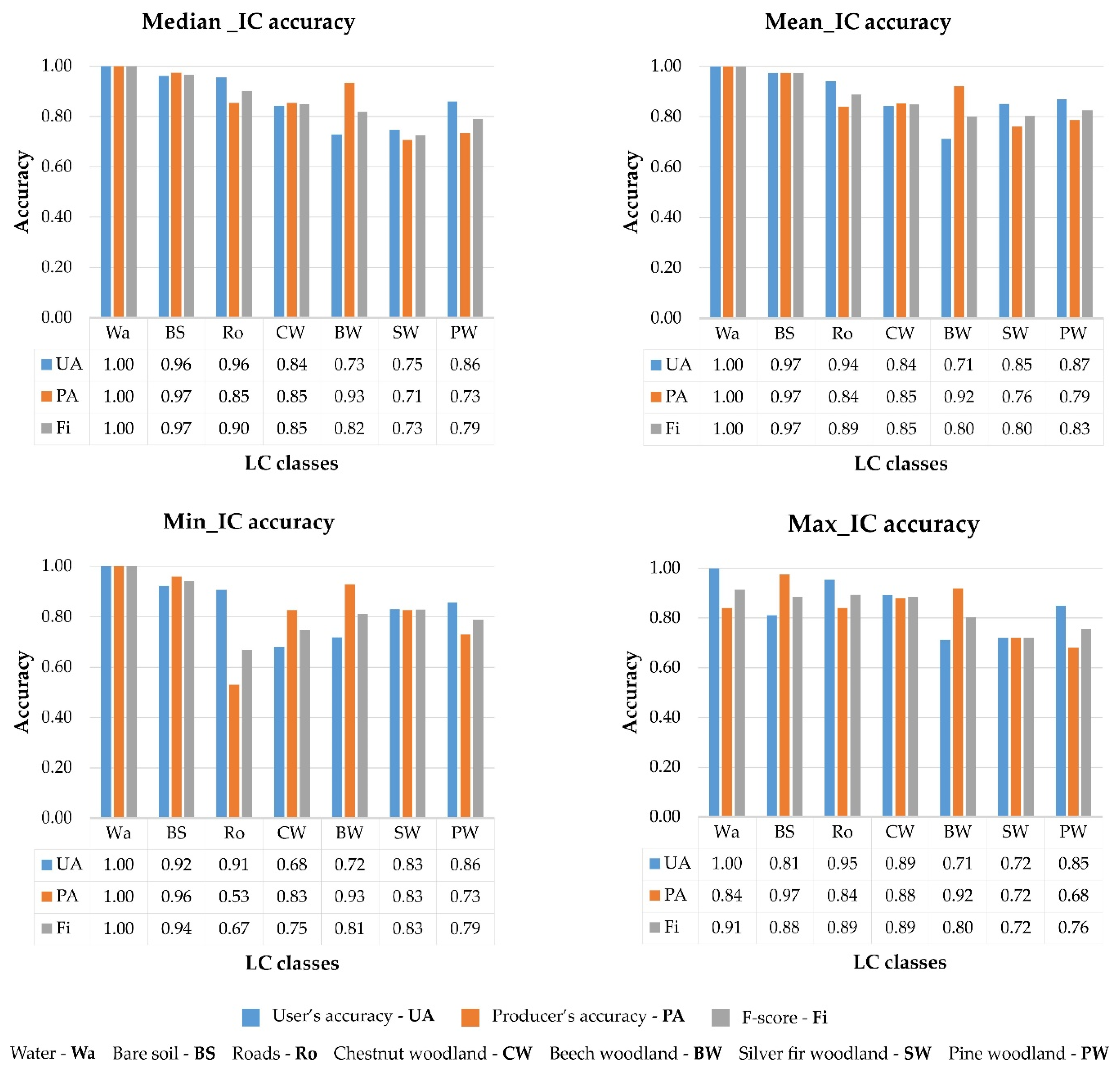
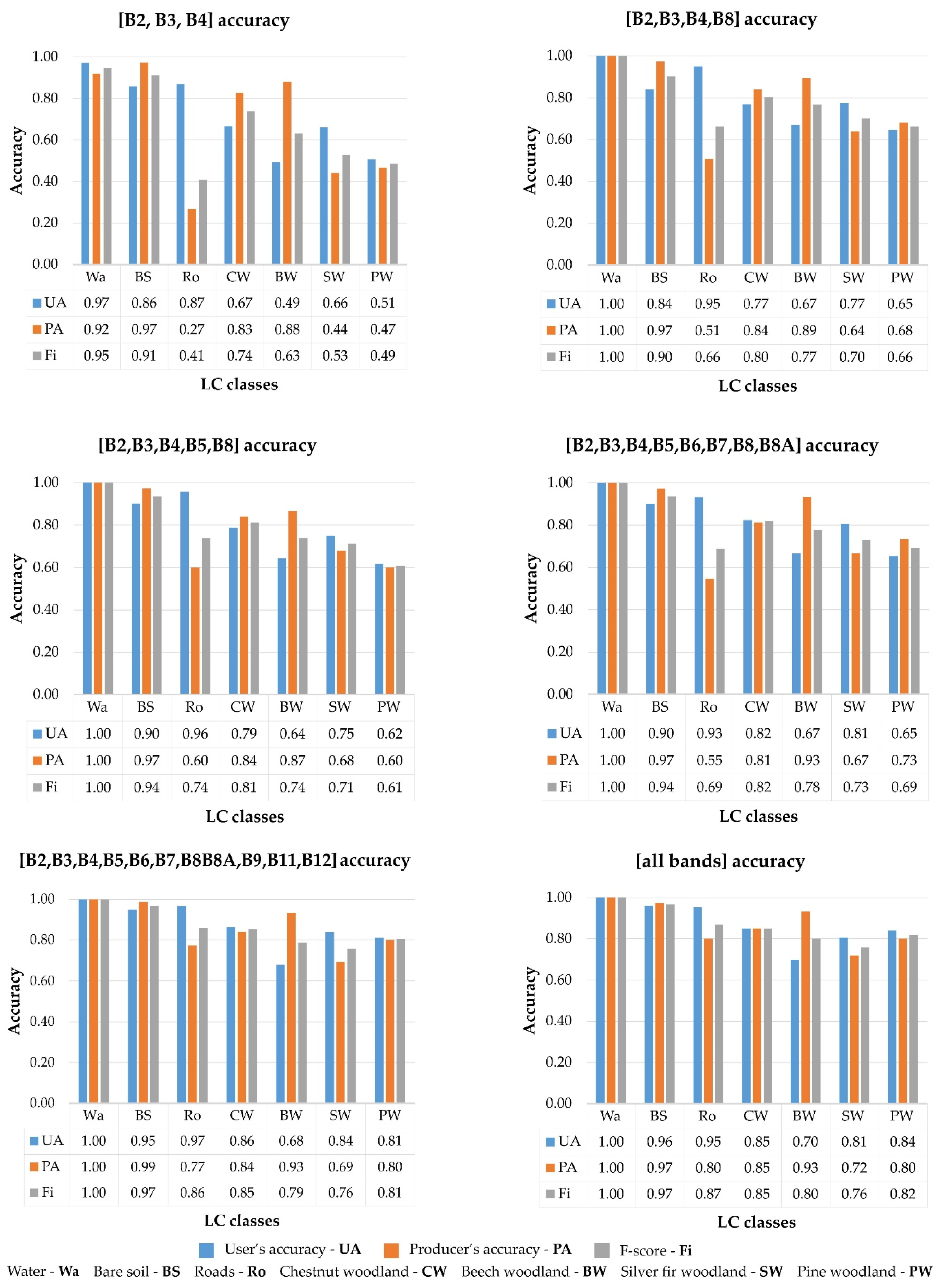
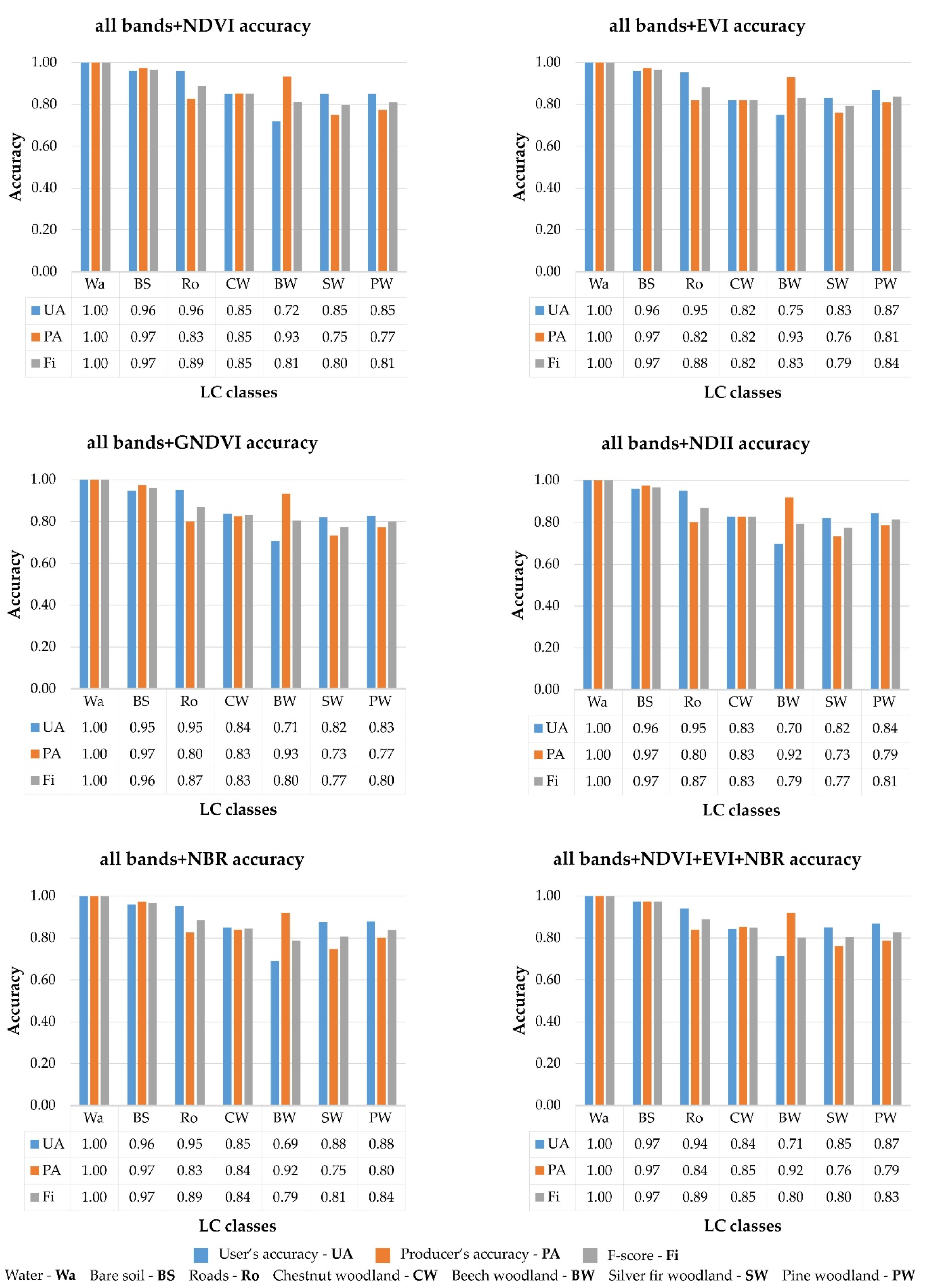
For each performed classification test, a measure of accuracy was performed, considering, as indicators, the overall accuracy (OA), the user’s accuracy (UA), and the producer’s accuracy (PA).
The OA is the total percentage of classification, given by the ratio between the number of correctly classified units and their total number [111], while UA and PA refer to single-class classification accuracies [112]. The UA is the ratio between correctly classified and all classified units in a given class, while the PA is the ratio between the number of correctly classified units and the number of validation units in a given class. The UA and PA were calculated, for each LC class, as the mean value of all LC classes, UAm (Equation (1)) and PAm (Equation (2)), respectively.
These accuracy measures were used to calculate the F-Score (Fi) [113,114] (Equation (3)) for each LC and the multi-class F-score (Fm) [115] (Equation (4)), the latter representing a measure of the entire classification process accuracy.
The F-score is the harmonic mean of recall and precision, which have the same meaning as PA and UA, respectively [87,101]:
UA m = i = 1 n U A n ,
PA m = i = 1 n P A n ,
F i = 2 P A U A P A + U A ,
F m = 2 P A m U A m P A m + U A m ,
where n is the number of LC classes.

3. Results

The image collection, after the filtering with the date and location process, consisted of 140 images. After applying the cloud cover threshold (maximum 5%), we obtained 33 elements, as follows: (i) 11 images for the winter season, (ii) 9 images for spring, (iii) 8 images for summer, and (iv) 5 images for autumn. Referring to the acquisition year, we retrieved 5 images for 2017 (starting from the end of March), 11 images for 2018, 11 images for 2019, and 6 images for the first half of 2020 (until the end of July).

3.1. Best Input Image Composite (IC)

This section reports the main results obtained after an extensive comparison of different variables (see Section 2.4.4), carried out through a trial-and-error approach, and aimed to highlight the best input image composite, in terms of image seasonality, reflectance bands, and VIs. Table 3 reports the main results of the seasonal IC choice step. The lowest accuracy values were attained when using the winter image composite (W_IC), with an OA of 0.72, UAm of 0.80, PAm of 0.72, and Fm of 0.76. The best result was obtained using the summer image composite (Su_IC), with an OA of 0.86, UAm of 0.87, PAm of 0.86, and Fm of 0.87. Focusing on single LC classes, the best performance was obtained when classifying Wa, with an Fi of 1. Considering the forest classes, the best and worst Fi scores were obtained using the autumn input composite (A_IC), for classes CW (0.89) and PW (0.33), respectively. UA, PA, and Fi values for each LC class and each examined IC, resulting from the trial-and-error approach, are displayed in Figure A1 (Appendix A).
Concerning the statistical operator adopted to reduce the image collection, the results are given in Table 4. The best accuracy value was obtained when reducing images with the mean. All used accuracy indicators were equal to 0.88. UA, PA, and Fi values for each LC class and each statistical operator, resulting from the trial-and-error approach, are displayed in Figure A2 (Appendix A).
Once we identified the best image composite, based on the accuracy results, we tested different band combinations for that image. We started by using only visible bands and then added NIR, RE, and SWIR bands.
The main results, shown in Table 5, highlight that the solution with all bands was the best input image, with an OOB error estimate of 0.01, an OA of 0.86, UAm and PAm equal to 0.87 and 0.86, respectively, and an Fm of 0.87. As expected, the lowest result was obtained using the visible bands (OA = 0.68, UAm = 0.72, PAm = 0.68, and Fm = 0.70).
The best-classified forest class was CW when using all bands, with an Fi of 0.85; while the worst score was reached for PW (0.49) when using just the visible bands. This image also gave the highest OOB error estimate (0.10). The UA, PA, and Fi values for each LC class and each spectral region investigated by the different bands, resulting from all the conducted iterations, are displayed in Figure A3 (Appendix A).
The computed VIs were added to the Su_IC all-bands image, and their contribution to the final result was investigated through the accuracy indicators and the OOB error estimate. The OOB error estimate remained stable (at 0.01) for all tests. Concerning the use of a single VI, the lowest accuracy values were reached using all bands and adding GNDVI or NDII with the same results for OA (0.86) and Fm (0.87), while the highest values were reached with the other three VIs, showing the same OA (0.87) and Fm (0.88). Although demonstrating identical mean accuracy values, these three combinations of bands and indices showed different Fi values for the various LC classes.
The best forest class score (0.85) was recorded for CW using all bands + NDVI, while the worst (0.79) was achieved for SW when adding the EVI layer to the IC and for BW adding the NBR. These three VIs were added together, reaching the best result with all accuracy indicators equal to 0.88.
Table 6 shows the main results of this step. Regarding this combination of bands and VIs, CW registered the highest Fi for forest classes, with a value of 0.85, while BW and SW had the lowest score (0.80). The UA, PA, and Fi values for each LC class with each VI taken into account are displayed in Figure A4 (Appendix A).
On the basis of the results of this process, the best input image for classification was obtained by reducing all the summer images using the mean statistical operator, considering all available Sentinel-2 bands, and adding NDVI, EVI, and NBR as VIs.

3.2. Classification Algorithms

As mentioned in Section 2.4.3, three machine learning algorithms were tested for their supervised pixel-based classification performance. RF obtained the best accuracy scores, with OA and Fm values of 0.88, followed by SVM, which registered values of 0.83 and 0.84 for OA and Fm, respectively.
The worst accuracy values were reached when performing classification with CART, obtaining an OA of 0.80 and an Fm of 0.79. According to the classification results (Figure 3), forest LC reached 6336.61 ha in RF, 6245.80 ha in SVM, and 6045.67 ha in CART. The BW class occupied the largest area, with a total surface of 3671.06 ha, 3332.77 ha, and 3895.65 ha for RF, SVM, and CART, respectively. The CW class occupied the least extent, ranging between 636.53 ha in RF, 404.43 ha in CART, and 334.81 ha in SVM.
Regarding the confusion matrices (Figure 4), it can be observed that all algorithms reached a satisfactory correspondence in classifying Wa (all validation points were correctly classified).
Considering forest LC classes, BW achieved the highest score in all classifiers, with a percentage of correctly assigned validation points of 93.33% for RF and CART and 90.67% for SVM. RF misassigned five points, assigning three to CW, one to Ro, and one to PW. SVM wrongly assigned five points to SW, one to PW, and one to Ro. CART misassigned two points to CW, two points to SW, and one point to BS.
RF reached the lowest score in classifying SW, misassigning 12 points to BW and 6 points to PW, reaching a percentage of correctly assigned points equal to 76% (57 points). SVM and CART highlighted PW class as the worst, with percentages of correctly assigned points of 61.33% and 66.67%, respectively. SVM wrongly assigned 16 points to SW, 12 points to BW, and 1 point to Ro; while CART erroneously assigned 13 points to SW, 11 points to BW, and 1 point to Ro.
Figure 5 shows the classified maps resulting from each adopted classifier and square plot.

4. Discussion

Unlike other similar studies relying on third-party software [75,76,116,117,118,119,120,121], we performed the entire workflow process inside the GEE cloud platform and used the JavaScript language to recall variables and functions in the code editor. This is a point of novelty of our research in this field. It is an attractive solution, because it allows different users with different technical devices of relatively low cost to obtain complete and satisfactory results, otherwise obtainable only by using external components that need background knowledge and a significant financial availability to buy high-performing PCs and/or commercial software. Our results show that the accuracy is generally high, compared to that obtained in other similar studies, and were completely in line with the accuracy highlighted in the review of Tamiminia et al. [14].
In previous studies, the data most used by other authors have been those from the Landsat constellation, followed by MODIS products (785 and 55 published papers, respectively, according to a review from GEE’s first use until 2020 [14]). We preferred the use of Sentinel-2 images instead, due to their better spatial resolution (10 m for visible and NIR bands, instead of 30 m for Landsat) and the narrow bandwidth in RE and NIR regions.
The classification accuracy is affected by the number and quality of training and validation points. We highlighted how the possibility of exploiting the computational potential of GEE makes it possible—quickly and without a need for storing big data—to use different seasonal ICs for the choice of training and validation points, which is generally considered the most delicate step in the classification process. We also highlighted that, when using the same set of reference data for training and validation, the input image composition choice led to different results. We tested different composition methods (seasonal composition strategies, statistical operators, band composition, and derived VIs information), in order to generate the best spectral input data for LC classification, investigating how this process may affect classification accuracy. Moreover, we tested the performance of three different classifiers (RF, SVM, and CART), using the same composite image as input.
According to the results summarised in Table 2, the worst accuracy results of W_IC may have been due to the non-simultaneous presence of all species on the ground, which generated errors in the LC classification, especially for BS and Ro classes. On the other hand, this composite was useful to discriminate coniferous training points, due to the absence of broadleaved trees in the scene. A progressive enhancement of accuracy values can be noticed with the other seasonal periods, representing the different phases of the senescence/growth cycle, reaching the best results in summer, when vegetative species are in their maximum growth period.
Although previous studies have approached the statistical operator issue in the image reduction process, highlighting median as the most-used [48,111], after testing different solutions with a trial-and-error approach, we obtained the best results using mean pixel values.
It is interesting to highlight that the progressive adding of Sentinel-2 bands to the RGB bands (Table 4) produced a decrease in the OOB error estimate and an increase in accuracy indicators (OA and Fm). This was because these bands add useful spectral information, facilitating the detection of different behaviours of remotely sensed objects, such as the chlorophyll response (in different portions of the NIR and RE wavelengths) or the response of water content (in SWIR wavelengths). A bottleneck of this process can be produced by the spectral similarity among co-occurring species, which could affect the results of a classification process based on multispectral instead of hyperspectral images [122]. Hyperspectral images are more difficult to obtain and require more background knowledge and, so far, require third-party software for their elaboration.
The use of VIs can improve classification accuracy. We tested five VIs (Table 5), three of which (NDVI, EVI, and NBR) produced a better result—in terms of increased accuracy—than the other two (GNDVI and NDII). This was probably due to the spectral behaviour of the species present in the study area and the characteristics of the selected input images. Moreover, we tested either a composition with these three best indices and a composition with all indices, highlighting that, for classification purposes, a correct choice of VIs is needed and should be preferred to the mere addition of derived indices.
Concerning the classification process, the choice of the three adopted classifiers was in line with the findings of the review of Taminia et al. [14], who reported RF, CART, and SVM as those which have been most adopted in previous GEE works (97, 26, and 21 published papers, respectively). Concerning the accuracy results, RF proved to be the best solution, in agreement with Rodriguez-Galiano et al. [123], who defined RF as being superior to other classifiers. Considering the total surface occupied by each LC class (Figure 4), the classified maps (Figure 5), and the composition in terms of percentage of each LC class (Figure 6), it can be observed that the three classifiers produced quite different results. In general, it is possible to see that, in SVM-classified maps (Figure 5), the typical salt-and-pepper effect of pixel-based classification is more accentuated than in the RF and CART maps, especially for Plot 1. RF and CART gave a similar result for the Wa class, while SVM overestimated this LC class by assigning it almost double the area indicated by the other two classifiers. Furthermore, SW was overestimated, while CW and BW were underestimated; mainly CW, which was assigned half the total surface assigned by RF. Concerning BS, the major overestimation was by CART, which assigned almost three-fold more surface assigned by RF. The total area occupied by the forest classes was overestimated either by SVM and CART. The reason for this is probably related to the intrinsic characteristics of RF which, as reported in the literature [124,125], is easy to train and is less sensitive to the quality of training data; unlike SVM, which is very sensitive to mislabelled pixels [126,127]. The results also showed that, in our case—having used the same set of training and validation data—the poor performance of SVM may be due to the remarkably heterogeneous nature of the identified plots. It is important to highlight that the obtained results were strongly linked to the spatial resolution of the available data in the GEE catalogue. It has been demonstrated that the results can be powerfully improved when using higher-resolution sensors [128].
In general, all classifiers produced an acceptable accuracy value, demonstrating the reliability of GEE as a tool enabling access to bulk data efficiently, which can also perform the entire classification process.

5. Conclusions

The main aim of this work was to test the potential of the GEE platform and Sentinel-2 time-series to classify LC in a mountainous natural national park, which included Natura 2000 sites hosting relevant protected forest habitats. Behind the entire work was the idea to exploit GEE to obtain a solid data collection, investigating how different uses and combinations of variables can improve the classification performance, without needing to rely on third-party software. Furthermore, the performance of different classification algorithms, in terms of classification accuracy, was compared and evaluated. By completing the entire classification process in a heterogeneous protected forest environment, such as that of the study area (Aspromonte National Park), we showed the reliability and versatility of GEE. Moreover, by efficiently managing a massive amount of RS data, thanks to its cloud architecture, it avoids using external and often commercial (i.e., expensive) software. In this work, high accuracy was reached thanks to the careful process of training and validation points collection, carried out by exploiting the opportunity of using different seasonal IC, and to the various iterations carried out during the trial-and-error approach to achieve the best input image. It highlighted the possibility to implement the entire classification process in this cloud environment, thus enabling worldwide dissemination of useful primary data for decision-making and planning processes, even in those countries with limited access to the most current technological resources. The only limitations remain the need for a good internet connection and the limited availability of data with suitable resolution in the catalogue, whose improvement in this direction is desirable for both researchers and practitioners.

Author Contributions

Conceptualization, S.P., F.S. and G.M.; methodology, S.P. and F.S.; software, S.P.; validation, S.P., F.S., S.D.F. and G.M.; formal analysis, S.P.; investigation, S.P. and F.S.; data curation, S.P.; writing—original draft preparation, S.P., F.S. and G.M.; writing—review and editing, S.P., F.S., S.D.F. and G.M.; visualization, S.P., S.D.F. and G.M.; supervision, S.D.F. and G.M. All authors have read and agreed to the published version of the manuscript.

Funding

The research of Dr. Salvatore Praticò was partially funded by the project “PON Research and Innovation 2014–2020—European Social Fund, Action I.2 Attraction and International Mobility of Researchers—AIM-1832342-1”. The research of Dr. Francesco Solano was partially funded by the project “FISR-MIUR Italian Mountain Lab”, and MIUR (Italian Ministry for Education, University and Research) initiative Department of Excellence (Law 232/2016).

Institutional Review Board Statement

Not applicable.

Informed Consent Statement

Not applicable.

Data Availability Statement

Sentinel-2 data are openly available via the Copernicus Open Access Hub and the Google Earth Engine. The GEE codes developed in this research are available, upon any reasonable request, by emailing the authors.

Conflicts of Interest

The authors declare no conflict of interest.

Appendix A

Figure A1. Seasonal image composition accuracy values.
Remotesensing 13 00586 g0a1
Figure A2. Accuracy values of the statistical operators adopted to reduce the images.
Remotesensing 13 00586 g0a2
Figure A3. Band composition accuracy values, according to the land-cover (LC) classes considered.
Remotesensing 13 00586 g0a3
Figure A4. Bands with vegetation indices (VIs) composition accuracy values, according to the land-cover (LC) classes considered.
Remotesensing 13 00586 g0a4

References

  1. Díaz Varela, R.A.; Ramil Rego, P.; Calvo Iglesias, S.; Muñoz Sobrino, C. Automatic habitat classification methods based on satellite images: A practical assessment in the NW Iberia coastal mountains. Environ. Monit. Assess. 2008, 144, 229–250. [Google Scholar] [CrossRef]
  2. European Commission. Commission Note on Establishment Conservation Measures for Natura 2000 Sites. Doc. Hab. 13-04/05. 2013. Available online: https://ec.europa.eu/environment/nature/natura2000/management/docs/commission_note/comNote conservation measures_EN.pdf (accessed on 7 January 2021).
  3. Di Fazio, S.; Modica, G.; Zoccali, P. Evolution Trends of Land Use/Land Cover in a Mediterranean Forest Landscape in Italy. In Proceedings of the Computational Science and Its Applications-ICCSA 2011, Part I, Lecture Notes in Computer Science, Santander, Spain, 20–23 June 2011; pp. 284–299. [Google Scholar]
  4. Modica, G.; Merlino, A.; Solano, F.; Mercurio, R. An index for the assessment of degraded Mediterranean forest ecosystems. For. Syst. 2015, 24, e037. [Google Scholar] [CrossRef] [Green Version]
  5. Modica, G.; Praticò, S.; Di Fazio, S. Abandonment of traditional terraced landscape: A change detection approach (a case study in Costa Viola, Calabria, Italy). Land Degrad. Dev. 2017, 28, 2608–2622. [Google Scholar] [CrossRef]
  6. Gómez, C.; White, J.C.; Wulder, M.A. Optical remotely sensed time series data for land cover classification: A review. ISPRS J. Photogramm. Remote Sens. 2016, 116, 55–72. [Google Scholar] [CrossRef] [Green Version]
  7. Modica, G.; Vizzari, M.; Pollino, M.; Fichera, C.R.; Zoccali, P.; Di Fazio, S. Spatio-temporal analysis of the urban–rural gradient structure: An application in a Mediterranean mountainous landscape (Serra San Bruno, Italy). Earth Syst. Dyn. 2012, 3, 263–279. [Google Scholar] [CrossRef] [Green Version]
  8. Kerr, J.T.; Ostrovsky, M. From space to species: Ecological applications for remote sensing. Trends Ecol. Evol. 2003, 18, 299–305. [Google Scholar] [CrossRef]
  9. Modica, G.; Pollino, M.; Solano, F. Sentinel-2 Imagery for Mapping Cork Oak (Quercus suber L.) Distribution in Calabria (Italy): Capabilities and Quantitative Estimation. In Proceedings of the International Symposium on New Metropolitan Perspectives, Reggio Calabria, Italy, 22–25 May 2018; pp. 60–67. [Google Scholar] [CrossRef]
  10. Lanucara, S.; Praticò, S.; Modica, G. Harmonization and Interoperable Sharing of Multi-Temporal Geospatial Data of Rural Landscapes. Available online: https://0-doi-org.brum.beds.ac.uk/10.1007/978-3-319-92099-3_7 (accessed on 7 January 2021).
  11. De Luca, G.; Silva, J.M.N.; Cerasoli, S.; Araújo, J.; Campos, J.; Di Fazio, S.; Modica, G. Object-based land cover classification of cork oak woodlands using UAV imagery and Orfeo Toolbox. Remote Sens. 2019, 11, 1238. [Google Scholar] [CrossRef] [Green Version]
  12. Fraser, R.H.; Olthof, I.; Pouliot, D. Monitoring land cover change and ecological integrity in Canada’s national parks. Remote Sens. Environ. 2009, 113, 1397–1409. [Google Scholar] [CrossRef]
  13. Borre, J.V.; Paelinckx, D.; Mücher, C.A.; Kooistra, L.; Haest, B.; De Blust, G.; Schmidt, A.M. Integrating remote sensing in Natura 2000 habitat monitoring: Prospects on the way forward. J. Nat. Conserv. 2011, 19, 116–125. [Google Scholar] [CrossRef]
  14. Amiminia, H.; Salehi, B.; Mahdianpari, M.; Quackenbush, L.; Adeli, S.; Brisco, B. Google Earth Engine for geo-big data applications: A meta-analysis and systematic review. ISPRS J. Photogramm. Remote Sens. 2020, 164, 152–170. [Google Scholar] [CrossRef]
  15. Steinhausen, M.J.; Wagner, P.D.; Narasimhan, B.; Waske, B. Combining Sentinel-1 and Sentinel-2 data for improved land use and land cover mapping of monsoon regions. Int. J. Appl. Earth Obs. Geoinf. 2018, 73, 595–604. [Google Scholar] [CrossRef]
  16. Cihlar, J. Land cover mapping of large areas from satellites: Status and research priorities. Int. J. Remote Sens. 2000, 21, 1093–1114. [Google Scholar] [CrossRef]
  17. Franklin, S.E.; Wulder, M.A. Remote sensing methods in medium spatial resolution satellite data land cover classification of large areas. Prog. Phys. Geogr. Earth Environ. 2002, 26, 173–205. [Google Scholar] [CrossRef]
  18. Chaves, M.E.D.; Picoli, M.C.A.; Sanches, I.D. Recent Applications of Landsat 8/OLI and Sentinel-2/MSI for Land Use and Land Cover Mapping: A Systematic Review. Remote Sens. 2020, 12, 3062. [Google Scholar] [CrossRef]
  19. Rogan, J.; Chen, D. Remote sensing technology for mapping and monitoring land-cover and land-use change. Prog. Plan. 2004, 61, 301–325. [Google Scholar] [CrossRef]
  20. Choudhury, A.M.; Marcheggiani, E.; Despini, F.; Costanzini, S.; Rossi, P.; Galli, A.; Teggi, S. Urban Tree Species Identification and Carbon Stock Mapping for Urban Green Planning and Management. Forests 2020, 11, 1226. [Google Scholar] [CrossRef]
  21. Nossin, J.J. A Review of: “Remote Sensing, theorie en toepassingen van landobservatie (Remoie Sensing theory and applications of land observation”). Edited by H, J. BUITEN and J. G. P. W. CLEVERS. Series ‘Dynamiek, indenting and bcheer van landelijke gebieden’, part 2. (Wageningen: Pudoe Publ., 1990.) [Pp. 504 ] (312 figs, 38 tables, 22 colour plates. 10 supplements, glossary.). Int. J. Remote Sens. 1991, 12, 2173. [Google Scholar] [CrossRef]
  22. Zhang, Y.; Xiao, X.; Wu, X.; Zhou, S.; Zhang, G.; Qin, Y.; Dong, J. A global moderate resolution dataset of gross primary production of vegetation for 2000–2016. Sci. Data 2017, 4, 170165. [Google Scholar] [CrossRef] [Green Version]
  23. Zhou, H.; Wang, C.; Zhang, G.; Xue, H.; Wang, J.; Wan, H. Generating a Spatio-Temporal Complete 30 m Leaf Area Index from Field and Remote Sensing Data. Remote Sens. 2020, 12, 2394. [Google Scholar] [CrossRef]
  24. Zhang, Y.L.; Song, C.H.; Band, L.E.; Sun, G.; Li, J.X. Reanalysis of global terrestrial vegetation trends from MODIS products: Browning or greening? Remote Sens. Environ. 2017, 191, 145–155. Available online: https://0-linkinghub-elsevier-com.brum.beds.ac.uk/retrieve/pii/S0034425716304977 (accessed on 7 January 2021). [CrossRef] [Green Version]
  25. Bolton, D.K.; Gray, J.M.; Melaas, E.K.; Moon, M.; Eklundh, L.; Friedl, M.A. Continental-scale land surface phenology from harmonized Landsat 8 and Sentinel-2 imagery. Remote Sens. Environ. 2020, 240, 111685. [Google Scholar] [CrossRef]
  26. Hansen, M.C.; Potapov, P.V.; Moore, R.; Hancher, M.; Turubanova, S.A.; Tyukavina, A.; Thau, D.; Stehman, S.V.; Goetz, S.J.; Loveland, T.R.; et al. High-resolution global maps of 21st-century forest cover change. Science 2013, 342, 850–853. [Google Scholar] [CrossRef] [PubMed] [Green Version]
  27. Pekel, J.-F.; Cottam, A.; Gorelick, N.; Belward, A.S. High-resolution mapping of global surface water and its long-term changes. Nature 2016, 540, 418–422. Available online: http://0-www-nature-com.brum.beds.ac.uk/articles/nature20584 (accessed on 7 January 2021). [CrossRef] [PubMed]
  28. Li, J.; Roy, D.P. A Global Analysis of Sentinel-2A, Sentinel-2B and Landsat-8 Data Revisit Intervals and Implications for Terrestrial Monitoring. Remote Sens. 2017, 9, 902. [Google Scholar]
  29. Weiers, S.; Bock, M.; Wissen, M.; Rossner, G. Mapping and indicator approaches for the assessment of habitats at different scales using remote sensing and GIS methods. Landsc. Urban Plan. 2004, 67, 43–65. [Google Scholar] [CrossRef]
  30. Cheţan, M.A.; Dornik, A.; Urdea, P. Analysis of recent changes in natural habitat types in the Apuseni Mountains (Romania), using multi-temporal Landsat satellite imagery (1986–2015). Appl. Geogr. 2018, 97, 161–175. [Google Scholar] [CrossRef]
  31. Bock, M.; Xofis, P.; Mitchley, J.; Rossner, G.; Wissen, M. Object-oriented methods for habitat mapping at multiple scales–Case studies from Northern Germany and Wye Downs, UK. J. Nat. Conserv. 2005, 13, 75–89. [Google Scholar] [CrossRef]
  32. Wang, F.; Xu, Y.J. Comparison of remote sensing change detection techniques for assessing hurricane damage to forests. Environ. Monit. Assess. 2009, 162, 311–326. [Google Scholar] [CrossRef]
  33. Pôças, I.; Cunha, M.; Pereira, L.S. Remote sensing based indicators of changes in a mountain rural landscape of Northeast Portugal. Appl. Geogr. 2011, 31, 871–880. [Google Scholar] [CrossRef]
  34. Pastick, N.J.; Wylie, B.K.; Wu, Z. Spatiotemporal analysis of Landsat-8 and Sentinel-2 data to support monitoring of dryland ecosystems. Remote Sens. 2018, 10, 791. [Google Scholar] [CrossRef] [Green Version]
  35. Vogelmann, J.E.; Xian, G.; Homer, C.G.; Tolk, B. Monitoring gradual ecosystem change using Landsat time series analyses: Case studies in selected forest and rangeland ecosystems. Remote Sens. Environ. 2012, 122, 92–105. [Google Scholar] [CrossRef] [Green Version]
  36. Simonetti, E.; Szantoi, Z.; Lupi, A.; Eva, H.D. First Results From the Phenology-Based Synthesis Classifier Using Landsat 8 Imagery. IEEE Geosci. Remote Sens. Lett. 2015, 12, 1496–1500. [Google Scholar] [CrossRef]
  37. Melaas, E.K.; Sulla-Menashe, D.; Gray, J.; Black, T.A.; Morin, T.H.; Richardson, A.D.; Friedl, M.A. Multisite analysis of land surface phenology in North American temperate and boreal deciduous forests from Landsat. Remote Sens. Environ. 2016, 186, 452–464. [Google Scholar] [CrossRef]
  38. Myneni, R.B.; Hall, F.G.; Sellers, P.J.; Marshak, A.L. Interpretation of spectral vegetation indexes. IEEE Trans. Geosci. Remote Sens. 1995, 33, 481–486. [Google Scholar] [CrossRef]
  39. Morisette, J.T.; Richardson, A.D.; Knapp, A.K.; Fisher, I.J.; Graham, A.E.; Abatzoglou, J.; Wilson, E.B.; Breshears, D.D.; Henebry, G.M.; Hanes, J.M.; et al. Tracking the rhythm of the seasons in the face of global change: Phenological research in the 21st century. Front. Ecol. Environ. 2009, 7, 253–260. [Google Scholar] [CrossRef] [Green Version]
  40. Solano, F.; Colonna, N.; Marani, M.; Pollino, M. Geospatial Analysis to Assess Natural Park Biomass Resources for Energy Uses in the Context of the Rome Metropolitan Area; Springer: Dordrecht, Netherlands, 2019; pp. 173–181. Available online: http://0-link-springer-com.brum.beds.ac.uk/10.1007/978-3-319-92099-3_21 (accessed on 7 January 2021).
  41. Lu, D.; Weng, Q. A survey of image classification methods and techniques for improving classification performance. Int. J. Remote Sens. 2007, 28, 823–870. [Google Scholar] [CrossRef]
  42. Jönsson, P.; Cai, Z.; Melaas, E.; Friedl, M.A.; Eklundh, L. A Method for Robust Estimation of Vegetation Seasonality from Landsat and Sentinel-2 Time Series Data. Remote Sens. 2018, 10, 635. [Google Scholar] [CrossRef] [Green Version]
  43. Thompson, S.D.; Nelson, T.A.; White, J.C.; Wulder, M.A. Mapping Dominant Tree Species over Large Forested Areas Using Landsat Best-Available-Pixel Image Composites. Can. J. Remote Sens. 2015, 41, 203–218. [Google Scholar] [CrossRef]
  44. Clark, M.L.; Aide, T.M.; Grau, H.R.; Riner, G. A scalable approach to mapping annual land cover at 250 m using MODIS time series data: A case study in the Dry Chaco ecoregion of South America. Remote Sens. Environ. 2010, 114, 2816–2832. [Google Scholar] [CrossRef]
  45. Wakulińska, M.; Marcinkowska-Ochtyra, A. Multi-Temporal Sentinel-2 Data in Classification of Mountain Vegetation. Remote Sens. 2020, 12, 2696. [Google Scholar] [CrossRef]
  46. Lehmann, E.A.; Wallace, J.F.; Caccetta, P.A.; Furby, S.L.; Zdunic, K. Forest cover trends from time series Landsat data for the Australian continent. Int. J. Appl. Earth Obs. Geoinf. 2013, 21, 453–462. [Google Scholar] [CrossRef]
  47. Gómez, C.; White, J.C.; Wulder, M.A.; Alejandro, P. Integrated Object-Based Spatiotemporal Characterization of Forest Change from an Annual Time Series of Landsat Image Composites. Can. J. Remote Sens. 2015, 41, 271–292. [Google Scholar] [CrossRef]
  48. Kollert, A.; Bremer, M.; Löw, M.; Rutzinger, M. Exploring the potential of land surface phenology and seasonal cloud free composites of one year of Sentinel-2 imagery for tree species mapping in a mountainous region. Int. J. Appl. Earth Obs. Geoinf. 2021, 94, 102208. [Google Scholar] [CrossRef]
  49. Li, S.; Dragicevic, S.; Anton, F.; Sester, M.; Winter, S.; Çöltekin, A.; Pettit, C.; Jiang, B.; Haworth, J.; Stein, A.; et al. Geospatial big data handling theory and methods: A review and research challenges. ISPRS J. Photogramm. Remote Sens. 2016, 115, 119–133. [Google Scholar] [CrossRef] [Green Version]
  50. Ma, Y.; Wu, H.; Wang, L.; Huang, B.; Ranjan, R.; Zomaya, A.Y.; Jie, W. Remote sensing big data computing: Challenges and opportunities. Futur. Gener. Comput. Syst. 2015, 51, 47–60. [Google Scholar] [CrossRef]
  51. Gorelick, N.; Hancher, M.; Dixon, M.; Ilyushchenko, S.; Thau, D.; Moore, R. Google Earth Engine: Planetary-scale geospatial analysis for everyone. Remote Sens. Environ. 2017, 202, 18–27. [Google Scholar] [CrossRef]
  52. Kumar, L.; Mutanga, O. Google Earth Engine Applications Since Inception: Usage, Trends, and Potential. Remote Sens. 2018, 10, 1509. [Google Scholar] [CrossRef] [Green Version]
  53. Mondal, P.; Liu, X. (Leon); Fatoyinbo, T.; Lagomasino, D. Evaluating Combinations of Sentinel-2 Data and Machine-Learning Algorithms for Mangrove Mapping in West Africa. Remote Sens. 2019, 11, 2928. [Google Scholar] [CrossRef] [Green Version]
  54. Chen, B.; Xiao, X.; Li, X.; Pan, L.; Doughty, R.; Ma, J.; Dong, J.; Qin, Y.; Zhao, B.; Wu, Z.; et al. A mangrove forest map of China in 2015: Analysis of time series Landsat 7/8 and Sentinel-1A imagery in Google Earth Engine cloud computing platform. ISPRS J. Photogramm. Remote Sens. 2017, 131, 104–120. [Google Scholar] [CrossRef]
  55. FForstmaier, A.; Shekhar, A.; Chen, J. Mapping of Eucalyptus in Natura 2000 Areas Using Sentinel 2 Imagery and Artificial Neural Networks. Remote Sens. 2020, 12, 2176. [Google Scholar] [CrossRef]
  56. Saah, D.; Johnson, G.; Ashmall, B.; Tondapu, G.; Tenneson, K.; Patterson, M.S.; Poortinga, A.; Markert, K.; Quyen, N.H.; Aung, K.S.; et al. Collect Earth: An online tool for systematic reference data collection in land cover and use applications. Environ. Model. Softw. 2019, 118, 166–171. [Google Scholar] [CrossRef]
  57. Tassi, A.; Vizzari, M. Object-Oriented LULC Classification in Google Earth Engine Combining SNIC, GLCM, and Machine Learning Algorithms. Remote Sens. 2020, 12, 3776. [Google Scholar] [CrossRef]
  58. Parks, S.A.; Holsinger, L.M.; Koontz, M.J.; Collins, L.; Whitman, E.; Parisien, M.; Loehman, R.A.; Barnes, J.L.; Bourdon, J.; Boucher, J.; et al. Giving Ecological Meaning to Satellite-Derived Fire Severity Metrics across North American Forests. Remote Sens. 2019, 11, 1735. [Google Scholar] [CrossRef] [Green Version]
  59. Senf, C.; Seidl, R. Mapping the forest disturbance regimes of Europe. Nat. Sustain. 2021, 4, 63–70. [Google Scholar] [CrossRef]
  60. Pérez-Romero, J.; Navarro-Cerrillo, R.M.; Palacios-Rodriguez, G.; Acosta, C.; Mesas-Carrascosa, F.J. Improvement of remote sensing-based assessment of defoliation of Pinus spp. caused by Thaumetopoea pityocampa Denis and Schiffermüller and related environmental drivers in Southeastern Spain. Remote Sens. 2019, 11, 1736. [Google Scholar] [CrossRef] [Green Version]
  61. Wang, C.; Jia, M.; Chen, N.; Wang, W. Long-Term Surface Water Dynamics Analysis Based on Landsat Imagery and the Google Earth Engine Platform: A Case Study in the Middle Yangtze River Basin. Remote Sens. 2018, 10, 1635. [Google Scholar] [CrossRef] [Green Version]
  62. De Lucia Lobo, F.; Souza-Filho, P.W.M.; Novo EML de, M.; Carlos, F.M.; Barbosa, C.C.F. Mapping Mining Areas in the Brazilian Amazon Using MSI/Sentinel-2 Imagery (2017). Remote Sens. 2018, 10, 1178. [Google Scholar] [CrossRef] [Green Version]
  63. Snapir, B.; Momblanch, A.; Jain, S.; Waine, T.; Holman, I.P. A method for monthly mapping of wet and dry snow using Sentinel-1 and MODIS: Application to a Himalayan river basin. Int. J. Appl. Earth Obs. Geoinf. 2019, 74, 222–230. [Google Scholar] [CrossRef] [Green Version]
  64. Hagenaars, G.; De Vries, S.; Luijendijk, A.P.; De Boer, W.P.; Reniers, A.J. On the accuracy of automated shoreline detection derived from satellite imagery: A case study of the sand motor mega-scale nourishment. Coast. Eng. 2018, 133, 113–125. [Google Scholar] [CrossRef]
  65. Liu, X.; Hu, G.; Chen, Y.; Li, X.; Xu, X.; Li, S.; Pei, F.; Wang, S. High-resolution multi-temporal mapping of global urban land using Landsat images based on the Google Earth Engine Platform. Remote Sens. Environ. 2018, 209, 227–239. [Google Scholar] [CrossRef]
  66. Ji, H.; Li, X.; Wei, X.; Liu, W.; Zhang, L.; Wang, L. Mapping 10-m Resolution Rural Settlements Using Multi-Source Remote Sensing Datasets with the Google Earth Engine Platform. Remote Sens. 2020, 12, 2832. [Google Scholar] [CrossRef]
  67. Callaghan, C.T.; Major, R.E.; Lyons, M.B.; Martin, J.M.; Kingsford, R.T. The effects of local and landscape habitat attributes on bird diversity in urban greenspaces. Ecosphere 2018, 9, e02347. [Google Scholar] [CrossRef] [Green Version]
  68. Caloiero, T.; Coscarelli, R.; Ferrari, E.; Mancini, M. Trend detection of annual and seasonal rainfall in Calabria (Southern Italy). Int. J. Clim. 2010, 31, 44–56. [Google Scholar] [CrossRef]
  69. Cameriere, P.; Caridi, D.; Crisafulli, A.; Spampinato, G. La carta della vegetazione reale del Parco Nazionale dell’Aspromonte (Italia meridionale). In Proceedings of the 97 Congresso Nazionale Della Società Botanica Italiana, Lecce, Italy, 24–27 September 2002. [Google Scholar]
  70. Modica, G.; Praticò, S.; Laudari, L.; Ledda, A.; Di Fazio, S.; De Montis, A. Design and implementation of multispecies ecological networks at the regional scale: Analysis and multi-temporal assessment. Remote Sens. under review.
  71. Spampinato, G.; Cameriere, P.; Caridi, D.; Crisafulli, A. Carta della biodiversità vegetale del Parco Nazionale dell’Aspromonte (Italia Meridionale). Quaderno di Botanica Ambientale Applicata 2009, 20, 3–36. [Google Scholar]
  72. Sánchez-Espinosa, A.; Schröder, C. Land use and land cover mapping in wetlands one step closer to the ground: Sentinel-2 versus landsat 8. J. Environ. Manag. 2019, 247, 484–498. [Google Scholar] [CrossRef] [PubMed]
  73. Munyati, C.; Balzter, H.; Economon, E. Correlating Sentinel-2 MSI-derived vegetation indices with in-situ reflectance and tissue macronutrients in savannah grass. Int. J. Remote Sens. 2020, 41, 3820–3844. [Google Scholar] [CrossRef]
  74. Schmitt, M.; Hughes, L.H.; Qiu, C.; Zhu, X.X. Aggregating Cloud-Free Sentinel-2 Images with Google Earth Engine. ISPRS Ann. Photogramm. Remote Sens. Spatial Inf. Sci. 2019, 4, 145–152. [Google Scholar] [CrossRef] [Green Version]
  75. Nguyen, M.D.; Baez-Villanueva, O.M.; Du Bui, D.; Nguyen, P.T.; Ribbe, L. Harmonization of Landsat and Sentinel 2 for Crop Monitoring in Drought Prone Areas: Case Studies of Ninh Thuan (Vietnam) and Bekaa (Lebanon). Remote Sens. 2020, 12, 281. [Google Scholar] [CrossRef] [Green Version]
  76. Zhang, W.; Brandt, M.; Wang, Q.; Prishchepov, A.V.; Tucker, C.J.; Li, Y.; Lyu, H.; Fensholt, R. From woody cover to woody canopies: How Sentinel-1 and Sentinel-2 data advance the mapping of woody plants in savannas. Remote Sens. Environ. 2019, 234, 111465. [Google Scholar] [CrossRef]
  77. Dong, J.; Xiao, X.; Chen, B.; Torbick, N.; Jin, C.; Zhang, G.; Biradar, C. Mapping deciduous rubber plantations through integration of PALSAR and multi-temporal Landsat imagery. Remote Sens. Environ. 2013, 134, 392–402. [Google Scholar] [CrossRef]
  78. Coppin, P.; Jonckheere, I.; Nackaerts, K.; Muys, B.; Lambin, E. Digital change detection methods in ecosystem monitoring: A review. Int. J. Remote Sens. 2004, 25, 1565–1596. [Google Scholar] [CrossRef]
  79. Rouse, J.W.; Hass, R.H.; Schell, J.A.; Deering, D.W. Monitoring Vegetation Systems in the Great Plains with ERTS. In Proceedings of the Third Earth Resources Technology Satellite (ERTS) Symposium, Washington, DC, USA, 10–14 December 1973; Volume 1, pp. 309–317. [Google Scholar]
  80. Gitelson, A.A.; Kaufman, Y.J.; Merzlyak, M.N. Use of a green channel in remote sensing of global vegetation from EOS-MODIS. Remote Sens. Environ. 1996, 58, 289–298. [Google Scholar] [CrossRef]
  81. Huete, A.; Didan, K.; Miura, T.; Rodriguez, E.P.; Gao, X.; Ferreira, L.G. Overview of the radiometric and biophysical performance of the MODIS vegetation indices. Remote Sens. Environ. 2002, 83, 195–213. [Google Scholar] [CrossRef]
  82. Kimes, D.; Markham, B.; Tucker, C.; McMurtrey, J. Temporal relationships between spectral response and agronomic variables of a corn canopy. Remote Sens. Environ. 1981, 11, 401–411. [Google Scholar] [CrossRef]
  83. Garcia, M.J.L.; Caselles, V. Mapping burns and natural reforestation using thematic Mapper data. Geocarto Int. 1991, 6, 31–37. [Google Scholar] [CrossRef]
  84. Raymond Hunt, E.; Rock, B.N.; Nobel, P.S. Measurement of leaf relative water content by infrared reflectance. Remote Sens. Environ. 1987, 22, 429–435. [Google Scholar] [CrossRef]
  85. Ji, L.; Zhang, L.; Wylie, B.K.; Rover, J. On the terminology of the spectral vegetation index (NIR − SWIR)/(NIR + SWIR). Int. J. Remote Sens. 2011, 32, 6901–6909. [Google Scholar] [CrossRef]
  86. Modica, G.; Messina, G.; De Luca, G.; Fiozzo, V.; Praticò, S. Monitoring the vegetation vigor in heterogeneous citrus and olive orchards. A multiscale object-based approach to extract trees’ crowns from UAV multispectral imagery. Comput. Electron. Agric. 2020, 175, 105500. [Google Scholar] [CrossRef]
  87. Solano, F.; Di Fazio, S.; Modica, G. A methodology based on GEOBIA and WorldView-3 imagery to derive vegetation indices at tree crown detail in olive orchards. Int. J. Appl. Earth Obs. Geoinf. 2019, 83, 101912. [Google Scholar] [CrossRef]
  88. Makinde, E.O.; Salami, A.T.; Olaleye, J.B.; Okewusi, O.C. Object Based and Pixel Based Classification Using Rapideye Satellite Imager of ETI-OSA, Lagos, Nigeria. Geoinform. FCE CTU 2016, 15, 59–70. [Google Scholar] [CrossRef]
  89. Praticò, S.; Di Fazio, S.; Modica, G. Multi Temporal Analysis of Sentinel-2 Imagery for Mapping Forestry Vegetation Types: A Google Earth Engine Approach; Springer: Dordrecht, Netherlands, 2021; pp. 1650–1659. Available online: http://0-link-springer-com.brum.beds.ac.uk/10.1007/978-3-030-48279-4_155 (accessed on 7 January 2021).
  90. Cihlar, J.; Latifovic, R.; Beaubien, J. A Comparison of Clustering Strategies for Unsupervised Classification. Can. J. Remote Sens. 2000, 26, 446–454. [Google Scholar] [CrossRef]
  91. Tou, J.T.; Gonzalez, R.C. Pattern Recognition Principles; Addison-Wesley Publishing Company: Boston, MA, USA, 1974. [Google Scholar]
  92. Hartigan, J.A.; Wong, M.A. A K-Means Clustering Algorithm. Appl. Stat. 1979, 28, 100. [Google Scholar] [CrossRef]
  93. Arthur, D.; Vassilvitskii, S. K-Means++: The Advantages of Careful Seeding. In Proceedings of the Eighteenth Annual ACM-SIAM Symposium on Discrete Algorithms, New Orleans, LA, USA, 7–9 January 2007; pp. 1027–1035. [Google Scholar]
  94. Vauhkonen, J.; Imponen, J. Unsupervised classification of airborne laser scanning data to locate potential wildlife habitats for forest management planning. Forests 2016, 89, 350–363. [Google Scholar] [CrossRef] [Green Version]
  95. Ma, L.; Cheng, L.; Li, M.; Liu, Y.; Ma, X. Training set size, scale, and features in Geographic Object-Based Image Analysis of very high resolution unmanned aerial vehicle imagery. ISPRS J. Photogramm. Remote Sens. 2015, 102, 14–27. [Google Scholar] [CrossRef]
  96. Jones, H.G.; Vaughan, R.A. Remote Sensing of Vegetation: Principles, Techniques, and Applications; Oxford University Press: Oxford, UK, 2010; 384p. [Google Scholar]
  97. Brovelli, M.A.; Sun, Y.; Yordanov, V. Monitoring Forest Change in the Amazon Using Multi-Temporal Remote Sensing Data and Machine Learning Classification on Google Earth Engine. ISPRS Int. J. Geo-Inf. 2020, 9, 580. [Google Scholar] [CrossRef]
  98. Abdi, A.M. Land cover and land use classification performance of machine learning algorithms in a boreal landscape using Sentinel-2 data. GIScience Remote Sens. 2020, 57, 1–20. [Google Scholar] [CrossRef] [Green Version]
  99. Maxwell, A.E.; Warner, T.A.; Fang, F. Implementation of machine-learning classification in remote sensing: An applied review. Int. J. Remote Sens. 2018, 39, 2784–2817. [Google Scholar] [CrossRef] [Green Version]
  100. Mardani, M.; Korrani, H.M.; De Simone, L.; Varas, S.; Kita, N.; Saito, T. Integration of Machine Learning and Open Access Geospatial Data for Land Cover Mapping. Remote Sens. 2019, 11, 1907. [Google Scholar] [CrossRef] [Green Version]
  101. Modica, G.; De Luca, G.; Messina, G.; Fiozzo, V.; Praticò, S. Comparison and assessment of different object-based classifications using machine learning algorithms and UAVs multispectral imagery in the framework of precision agriculture. Remote Sens. under review.
  102. Breiman, L. Random forests. Mach. Learn. 2001, 45, 5–32. [Google Scholar] [CrossRef] [Green Version]
  103. Cutler, D.R.; Edwards, T.C.; Beard, K.H.; Cutler, A.; Hess, K.T.; Gibson, J.; Lawler, J.J. Random Forests for Classification in Ecology. Ecology 2007, 88, 2783–2792. [Google Scholar] [CrossRef]
  104. Breiman, L.; Friedman, J.H.; Olshen, R.A.; Stone, C.J. Classification and Regression Trees [Internet]. Available online: https://www.taylorfrancis.com/books/9781351460491 (accessed on 7 January 2021).
  105. Loh, W. Classification and regression trees. Wiley Interdiscip. Rev. Data Min. Knowl. Discov. 2011, 1, 14–23. [Google Scholar] [CrossRef]
  106. Bishop, C. Pattern Recognition and Machine Learning; Springer: New York, NY, USA, 2006; p. 738. [Google Scholar]
  107. Cortes, C.; Vapnik, V. Support-Vector Networks. Mach. Learn. 1995, 20, 273–297. [Google Scholar] [CrossRef]
  108. Vapnik, V. Statistical Learning Theory; New York John Wiley and Sons: New York, NY, USA, 1998. [Google Scholar]
  109. Huang, C.; Davis, L.S.; Townshend, J.R.G. An assessment of support vector machines for land cover classification. Int. J. Remote Sens. 2002, 23, 725–749. [Google Scholar] [CrossRef]
  110. Phan, T.N.; Kuch, V.; Lehnert, L.W. Land Cover Classification using Google Earth Engine and Random Forest Classifier—The Role of Image Composition. Remote Sens. 2020, 12, 2411. [Google Scholar] [CrossRef]
  111. Congalton, R.G.; Green, K. Assessing the Accuracy of Remotely Sensed Data; CRC Press: Boca Raton, FL, USA, 2019. [Google Scholar]
  112. Story, M.; Congalton, R.G. Remote Sensing Brief Accuracy Assessment: A User’s Perspective. Photogramm. Eng. Remote Sens. 1986, 52, 397–399. [Google Scholar]
  113. Goutte, C.; Gaussier, E. A Probabilistic Interpretation of Precision, Recall and F-Score, with Implication for Evaluation; Springer: Berlin/Heidelberg, Germany, 2005; pp. 345–359. [Google Scholar] [CrossRef]
  114. Sokolova, M.; Japkowicz, N.; Szpakowicz, S. Beyond Accuracy, F-Score and ROC: A Family of Discriminant Measures for Performance Evaluation; Springer: Berlin/Heidelberg, Germany, 2006; pp. 1015–1021. [Google Scholar] [CrossRef] [Green Version]
  115. Sokolova, M.; Lapalme, G. A systematic analysis of performance measures for classification tasks. Inf. Process. Manag. 2009, 45, 427–437. [Google Scholar] [CrossRef]
  116. Hauser, L.T.; An Binh, N.; Viet Hoa, P.; Hong Quan, N.; Timmermans, J. Gap-Free Monitoring of Annual Mangrove Forest Dynamics in Ca Mau Province, Vietnamese Mekong Delta, Using the Landsat-7-8 Archives and Post-Classification Temporal Optimization. Remote Sens. 2020, 12, 3729. [Google Scholar] [CrossRef]
  117. Hird, J.N.; DeLancey, E.R.; McDermid, G.J.; Kariyeva, J. Google earth engine, open-access satellite data, and machine learning in support of large-area probabilisticwetland mapping. Remote Sens. 2017, 9, 1315. [Google Scholar] [CrossRef] [Green Version]
  118. Regan, S.; Gill, L.; Regan, S.; Naughton, O.; Johnston, P.; Waldren, S.; Ghosh, B. Mapping Vegetation Communities Inside Wetlands Using Sentinel-2 Imagery in Ireland. Int. J. Appl. Earth Obs. Geoinf. 2020, 88, 102083. [Google Scholar] [CrossRef]
  119. Vivekananda, G.N.; Swathi, R.; Sujith, A. Multi-temporal image analysis for LULC classification and change detection. Eur. J. Remote Sens. 2020, 1, 1–11. [Google Scholar] [CrossRef]
  120. Tong, X.; Brandt, M.; Hiernaux, P.; Herrmann, S.; Rasmussen, L.V.; Rasmussen, K.; Tian, F.; Tagesson, T.; Zhang, W.; Fensholt, R. The forgotten land use class: Mapping of fallow fields across the Sahel using Sentinel-2. Remote Sens. Environ. 2020, 239, 111598. [Google Scholar] [CrossRef]
  121. Johansen, K.; Phinn, S.; Taylor, M. Mapping woody vegetation clearing in Queensland, Australia from Landsat imagery using the Google Earth Engine. Remote Sens. Appl. Soc. Environ. 2015, 1, 36–49. [Google Scholar] [CrossRef]
  122. Somers, B.; Asner, G.P. Tree species mapping in tropical forests using multi-temporal imaging spectroscopy: Wavelength adaptive spectral mixture analysis. Int. J. Appl. Earth Obs. Geoinf. 2014, 31, 57–66. [Google Scholar] [CrossRef]
  123. Rodriguez-Galiano, V.; Ghimire, B.; Rogan, J.; Chicaolmo, M.; Rigol-Sanchez, J. An assessment of the effectiveness of a random forest classifier for land-cover classification. ISPRS J. Photogramm. Remote Sens. 2012, 67, 93–104. [Google Scholar] [CrossRef]
  124. Belgiu, M.; Drăgu, L. Random forest in remote sensing: A review of applications and future directions. ISPRS J. Photogramm. Remote Sens. 2016, 114, 24–31. [Google Scholar] [CrossRef]
  125. Mahdianpari, M.; Salehi, B.; Mohammadimanesh, F.; Motagh, M. Random forest wetland classification using ALOS-2 L-band, RADARSAT-2 C-band, and TerraSAR-X imagery. ISPRS J. Photogramm. Remote Sens. 2017, 130, 13–31. [Google Scholar] [CrossRef]
  126. Mountrakis, G.; Im, J.; Ogole, C. Support vector machines in remote sensing: A review. ISPRS J. Photogramm. Remote Sens. 2011, 66, 247–259. [Google Scholar] [CrossRef]
  127. Holloway, J.; Mengersen, K. Statistical Machine Learning Methods and Remote Sensing for Sustainable Development Goals: A Review. Remote Sens. 2018, 10, 1365. [Google Scholar] [CrossRef] [Green Version]
  128. Messina, G.; Peña, J.M.; Vizzari, M.; Modica, G. A Comparison of UAV and Satellites Multispectral Imagery in Monitoring Onion Crop. An Application in the ‘Cipolla Rossa di Tropea’ (Italy). Remote Sens. 2020, 12, 3424. [Google Scholar] [CrossRef]
Figure 1. Workflow of the presented method. The first part shows the image pre-processing step to obtain the time-series. The second part shows all image processing steps to obtain image composites. The third part shows all the classification process components, while the fourth concerns the accuracy comparison step to obtain the final output (the last step). List of abbreviations: NDVI (normalised difference vegetation index); GNDVI (green normalised difference vegetation index); EVI (enhanced vegetation index); NBR (normalised burn ratio); NDII (normalised difference infrared index); DEM (digital elevation model); CART (classification and regression tree); RF (random forest); SVM (support vector machine); OA (overall accuracy).
Remotesensing 13 00586 g001
Figure 2. Geographical location of the study area— natural Aspromonte National Park—with the boundaries of the Natura 2000 sites considered. The three defined plots (Plot_01, Plot_02, and Plot_03) are shown as Sentinel-2 false colour images (RGB 7,3,2 band composition).
Remotesensing 13 00586 g002
Figure 3. Total classified surface for each adopted classifier (RF: random forest; SVM: support vector machine; CART: classification and regression tree) and for each adopted land-cover (LC) class (Wa: water; BS: bare soil; Ro: roads; CW: chestnut woodland; BW: beech woodland; SW: silver fir woodland; PW: pine woodland).
Remotesensing 13 00586 g003
Figure 4. Confusion matrices and charts for each adopted classifier (RF: random forest; SVM: support vector machine; CART: classification and regression tree) and for each adopted land-cover (LC) class (Wa: water; BS: bare soil; Ro: roads; CW: chestnut woodland; BW: beech woodland; SW: silver fir woodland; PW: pine woodland).
Remotesensing 13 00586 g004
Figure 5. The maps resulting from each adopted classifier (RF: random forest; SVM: support vector machine; CART: classification and regression tree), in rows and, for each square plot, in columns.
Remotesensing 13 00586 g005
Figure 6. Percentages of total area occupied by each LU/LC class (Wa: water; BS: bare soil; Ro: roads; CW: chestnut woodland; BW: beech woodland; SW: silver fir woodland; PW: pine woodland) for each classifier: random forest (RF), support vector machine (SVM), and classification and regression tree (CART).
Remotesensing 13 00586 g006
Table 1. Bands characteristics of Sentinel-2 multispectral sensors.
Band Sentinel-2 ASentinel-2 BGSD
[m]
BandwidthCentral WavelengthBandwidthCentral Wavelength
[nm][nm][nm][nm]
121442.721442.260
266492.466492.110
336559.836559.010
431664.631664.910
515704.116703.820
615740.515739.120
720782.820779.720
8106832.8106832.910
8A21864.721864.020
920945.121943.260
10311373.5301376.960
11911613.7941610.420
121752202.41852185.720
Table 2. Vegetation indices (VIs) adopted in this work and computed in the Google Earth Engine (GEE).
Vegetation Index (VI)FormulaReference
Normalised Difference Vegetation Index (NDVI) N I R ρ 842 R e d ρ 665 N I R ρ 842 + R e d ρ 665 [79]
Green Normalised Difference Vegetation Index (GNDVI) N I R ρ 842 G r e e n ρ 560 N I R ρ 842 + G r e e n ρ 560 [80]
Enhanced Vegetation Index (EVI) G N I R ρ 842 R e d ρ 665 N I R ρ 842 + C 1 R e d ρ 665 C 2 B l u ρ 490 + L [81]
Normalised Difference Infrared Index (NDII) N I R ρ 842 S W I R ρ 1610 N I R ρ 842 + S W I R ρ 1610 [82]
Normalised Burn Ratio (NBR) N I R ρ 842 S W I R ρ 2190 N I R ρ 842 + S W I R ρ 2190 [83]
Table 3. The different combinations of image composites (ICs) tested in the first step of the proposed method (i.e., best input image composite selection). The obtained overall accuracy (OA) and multi-class F-score (Fm) are reported for each tested IC. Moreover, the third column reports the out-of-bag (OOB) error estimate values for the random forest (RF) algorithm.
Input ImageAccuracyOOB Error Estimate
All_ICOA 0.79
Fm 0.80
0.01
W_ICOA 0.72
Fm 0.76
0.01
Sp_ICOA 0.82
Fm 0.82
0.02
Su_ICOA 0.86
Fm 0.87
0.01
A_ICOA 0.77
Fm 0.79
0.02
Table 4. The different combinations of bands adopted for the Su_IC input image with accuracy information of overall accuracy (OA) and multi-class F-score (Fm). Moreover, the out-of-bag (OOB) error estimate values for the RF algorithm are reported.
StatisticsAccuracyOOB Error Estimate
meanOA 0.88
Fm 0.88
0.01
medianOA 0.86
Fm 0.86
0.01
minimumOA 0.82
Fm 0.83
0.02
maximumOA 0.84
Fm 0.84
0.01
Table 5. The different combinations of bands adopted on the summer image composite (Su_IC) and the obtained accuracy information, expressed as overall accuracy (OA) and multi-class F-score (Fm). Moreover, the out-of-bag (OOB) error estimate values for the random forest (RF) algorithm are reported.
Input BandsAccuracyOOB Error Estimate
Visible
(B2, B3, B4)
OA 0.68
Fm 0.70
0.10
Visible + NIR
(B2, B3, B4, B8)
OA 0.79
Fm 0.80
0.06
Visible + RE + NIR
(B2, B3, B4, B5, B8)
OA 0.79
Fm 0.80
0.05
Visible + all REs + all NIRs
(B2, B3, B4, B5, B6, B7, B8, B8A)
OA 0.81
Fm 0.82
0.03
Visible + all REs + all NIRs+ all SWIRs
(B2, B3, B4, B5, B6, B7, B8, B8A, B9, B11, B12)
OA 0.85
Fm 0.84
0.02
All bandsOA 0.86
Fm 0.87
0.01
Table 6. The overall accuracy (OA) and multi-class F-scores (Fm) obtained with different combinations of bands adopted on the summer image composite (Su_IC). Moreover, the out-of-bag (OOB) error estimate values for the random forest (RF) algorithm are reported.
Vegetation IndicesAccuracyOOB Error Estimate
NDVIOA 0.87
Fm 0.88
0.01
EVIOA 0.87
Fm 0.88
0.01
GNDVIOA 0.86
Fm 0.87
0.01
NDIIOA 0.86
Fm 0.87
0.01
NBROA 0.87
Fm 0.88
0.01
NDVI + EVI + NBROA 0.88
Fm 0.88
0.01
All indicesOA 0.87
Fm 0.87
0.01
Publisher’s Note: MDPI stays neutral with regard to jurisdictional claims in published maps and institutional affiliations.

