
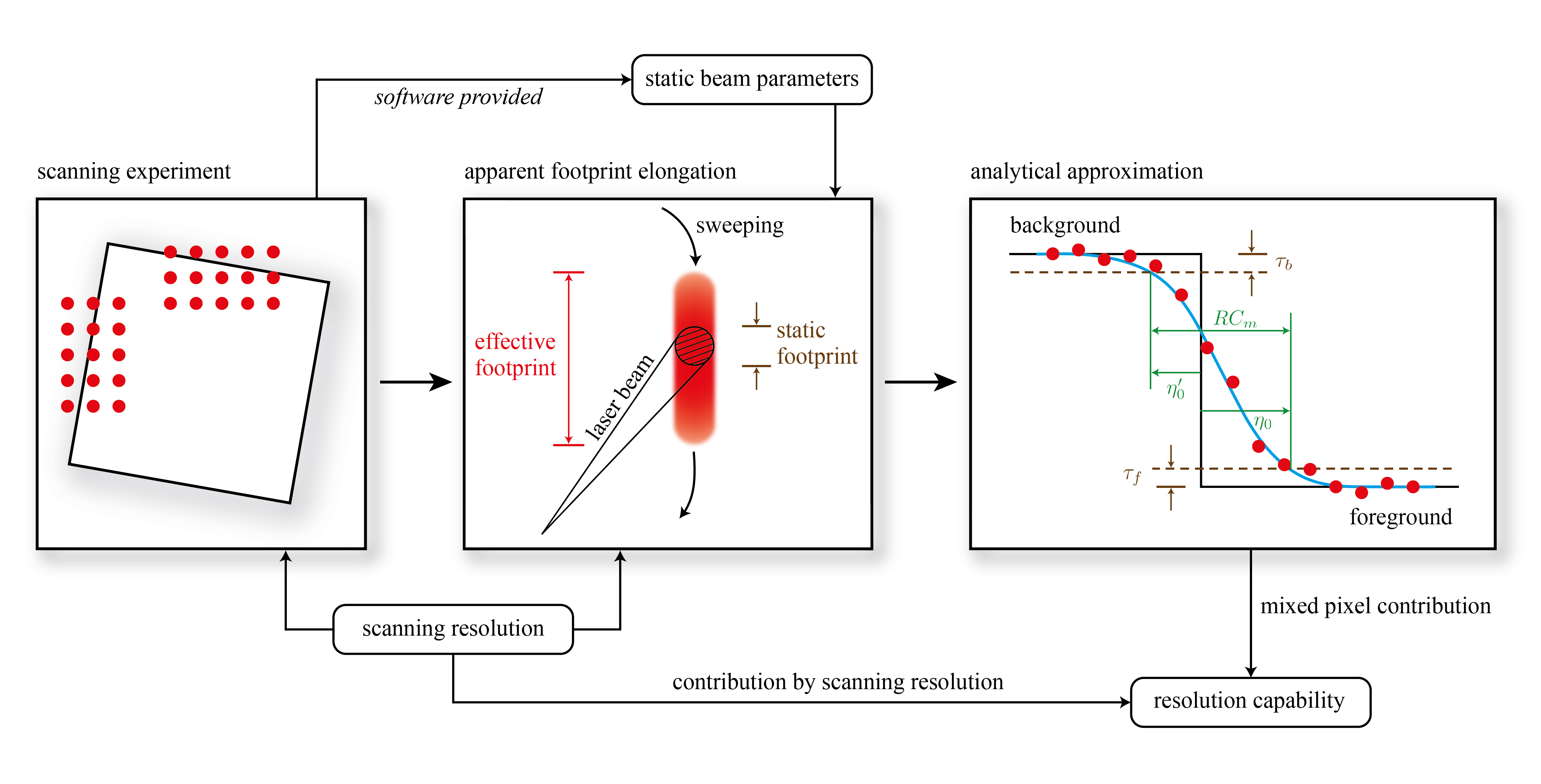
A Modeling Approach for Predicting the Resolution Capability in Terrestrial Laser Scanning


Institute of Geodesy and Photogrammetry, ETH Zurich, 8093 Zurich, Switzerland
*
Author to whom correspondence should be addressed.
Remote Sens. 2021, 13(4), 615; https://0-doi-org.brum.beds.ac.uk/10.3390/rs13040615
Submission received: 8 January 2021
/
Revised: 3 February 2021
/
Accepted: 5 February 2021
/
Published: 9 February 2021
(This article belongs to the Special Issue 3D Modelling from Point Cloud: Algorithms and Methods)
Abstract
:The minimum size of objects or geometrical features that can be distinguished within a laser scanning point cloud is called the resolution capability (RC). Herein, we develop a simple analytical expression for predicting the RC in angular direction for phase-based laser scanners. We start from a numerical approximation of the mixed-pixel bias which occurs when the laser beam simultaneously hits surfaces at grossly different distances. In correspondence with previous literature, we view the RC as the minimum angular distance between points on the foreground and points on the background which are not (severely) affected by a mixed-pixel bias. We use an elliptical Gaussian beam for quantifying the effect. We show that the surface reflectivities and the distance step between foreground and background have generally little impact. Subsequently, we derive an approximation of the RC and extend it to include the selected scanning resolution, that is, angular increment. We verify our model by comparison to the resolution capabilities empirically determined by others. Our model requires parameters that can be taken from the data sheet of the scanner or approximated using a simple experiment. We describe this experiment herein and provide the required software on GitHub. Our approach is thus easily accessible, enables the prediction of the resolution capability with little effort and supports assessing the suitability of a specific scanner or of specific scanning parameters for a given application.

1. Introduction
Each distance measurement produced by a laser scanner is a weighted average over the footprint, that is, over the surfaces illuminated quasi-simultaneously by the beam. As the scanner sweeps the beam across the environment to create a 3d point cloud, it unavoidably also illuminates surfaces with vastly different distances at some times. The coordinates of the corresponding points may be corrupted by biases well above the precision of the instrument [1]. This so-called mixed pixel effect is often observed near edges in terrestrial laser scanning (TLS) [2,3,4,5,6,7]. Several researchers have studied the effect and proposed algorithms to detect or filter out mixed pixels in point clouds [8,9,10,11,12,13,14].
A practically relevant aspect related to mixed pixels is the resolution capability (RC, ) of a scanner. This is the minimum size in angular direction of an object or geometrical feature that can be distinguished within the point cloud [15]. Obviously, the RC depends on the sampling interval (or scanning resolution, ), that is, the angular distance between neighboring points in the point cloud, because there must be at least one point on its surface to distinguish an object, and thus . Due to the distance averaging within the footprint also depends on the size of the footprint and thus on the beam parameters [16]. In fact, the object must be big enough such that there is at least one point on its surface which is not a mixed pixel. We may expect that the (user selected) scanning resolution dominates if it is much larger than the footprint whereas the mixed pixel effect dominates otherwise.
The resolution capability of laser scanners has been investigated experimentally by several authors. Reference [17] carried out a general analysis of various indicators of laser scanner accuracy based on data acquired experimentally with commercial scanners on specifically designed targets, including observations of the influence of mixed pixels on effective resolution and edge effects. References [16,18] used optical transfer function analysis to define a unified metric that accounts for the joint impact of scanning resolution and beam size, demonstrating that the effective RC is only reliably defined by the selected scanning resolution when the latter is much larger than the laser footprint. Reference [19] evaluated the interplay between scanning resolution and beam divergence empirically to derive practical insights for the appropriate choice of the scanning resolution and scanning configuration in view of the required level of detail of the resulting point cloud. Following the approach of [17] and using ad-hoc targets [15,20,21] focused on extensive experimental investigations of the RC of specific instruments, providing practical recommendations about the suitability of certain scanners and settings for given requirements in terms of level of geometric details represented by the point cloud.
Herein, we complement these investigations by providing an analytical expression for predicting the angular resolution capability as a function of beam properties and additionally relevant parameters, namely distance, distance noise, surface reflectivities and modulation wavelength. We focus on phase-based LiDAR (light detection and ranging) which uses modulated continuous waves. This technology is the backbone of some of the most precise commercially available terrestrial laser scanners for short to medium ranges, requires no algorithmic design choices like signal detection thresholds or full wave-form analysis potentially affecting the RC, and cannot be tuned to separate multiple reflections within the same beam. We derive the analytical expression from a numerical model of the mixed pixel effect and simplify it by focusing on the most influential parameters. Our main contribution with respect to previous investigations on RC lies in providing a simple expression which bounds the RC that can be expected from a certain scanner and scanning scenario, and which requires only parameters that can in most cases be obtained directly from the manufacturer’s specifications or simply approximated.
Our models of mixed pixels and RC are based on the assumption of a Gaussian beam [22,23,24]. If the beam waist diameter and the beam divergence are given in the instrument’s data sheet, the resolution capability can be predicted with practically useful accuracy using only the data sheet and the equations given herein. However, currently the data sheets rarely contain these values or the necessary quantities allowing to calculate them unambiguously. As an additional contribution, we therefore introduce a simple procedure to derive sufficient approximations of the beam parameters experimentally, from scans across an edge between a planar foreground and a planar background. The MATLAB functions for calculating the beam parameters from the scans are provided on GitHub: https://github.com/ChaudhrySukant/BeamProfiling (accessed on 2 February 2021).
The paper is structured as follows—Section 2 briefly presents the mathematical model of phase-based LiDAR measurements. In Section 3 we derive an analytical model for the mixed pixel effect at a single edge between parallel planar foreground and background of possibly different reflectivity. We also establish the relation to the resolution capability. In Section 4 we show the experimental setup for a mixed pixel analysis and for determining the relevant beam parameters. We briefly refer to the numerical simulation framework used for validation of the simplified analytical expressions. Section 5 shows experimental results comparing predicted and observed mixed pixel effects. In Section 6 we compare the RC for three scanners and different settings obtained from our analytical model to the results reported by [15,21] who used a specially designed target for an experimental investigation. The conclusions are given in Section 7.
2. Phase-Based LiDAR
Phase-based LiDAR systems estimate the distance to the illuminated targets from the accumulated phase of radio-frequency tones modulated onto a continuous-wave (CW) laser [25]. The phase is an indirect observation of the propagation time of the optical probing signal. Assuming that the measurement refers to a single point at the euclidean distance d from the mechanical zero of the instrument, the phase observation at a certain modulation wavelength can be written as
where represents the measurement error and the systematic distance offset between the internal phase reference of the instrument and its mechanical zero, compensated by calibration. The estimated distance to the target can be derived from this phase observation as
where is the (unknown) number of full cycles covered by the modulation wavelength .
For real LiDAR measurements the beam is actually reflected by a finite patch of surface rather than at a single point. The observed phase therefore represents the weighted contributions of the signals reflected across the beam footprint on the surface. These contributions experience different delays and attenuation depending on the surface geometry and reflectance properties across . Considering the phasor sum of all contributions, the observed phase can be expressed as
where the quadra- and in-phase components and are actually measured by the instrument [26,27]. They result from mixing the received signal with an attenuated copy of the simultaneously emitted signal and of a delayed version of it, as is for example, also known from GPS carrier phase tracking, see for example, [28]. These components are functions of the distances and reflected optical powers within , such that
where and are the measurement errors, and the footprint is expressed as the subset of angles and (in orthogonal directions) from the beam axis for which the irradiance on the surface is relevant.
We will further specify and simplify this general model for the phase observations in the next section by considering only a limited number of reflected contributions in order to derive a model of the mixed-pixels bias. A more detailed explanation of the phase-based LiDAR measurement process can be found in [27].
As is apparent from Equations (1) and (2), the number of full cycles is unknown, making phase-based distance measurements inherently ambiguous for ranges larger than . This is practically solved by combining two or more modulation wavelengths and thus extending the overall unambiguous range across the complete measurement range of the instrument. We base our analysis herein on an incremental ambiguity resolution approach, that represents the simplest solution for multi-wavelength distance measurement. This approach relies on using a longer wavelength to solve the cycle ambiguity of the (immediately next) shorter wavelength, see for example, [25]. The actually used modulation wavelengths of modern laser scanners are usually not communicated by the manufacturers, but the shortest ones may be expected to be on the order of about , as established for electronic distance meters, [25] and also indicated by the values reported about an older Faro scanner in [12] (). It requires the uncertainty of the measurement at the longer wavelength to be less than the shorter wavelength. Once unambiguous, the final measurement is uniquely defined by the shortest wavelength, which provides the highest resolution and precision.
Given a phase observation at a modulation wavelength where is the maximum possible range of the instrument, and ignoring for simplicity, an unambiguous distance estimate can be directly obtained from
This measurement is then used to select the number of full cycles of the shorter wavelength that provides the highest agreement, that is,
with being the observed phase at , and larger than the uncertainty of . This enables an absolute distance estimation based on the smaller wavelength , therefore more precise than under the same measurement conditions.
This process can be carried out sequentially with more than two wavelengths. The choice of wavelengths and ambiguity resolution approach by the manufacturer is a trade-off between maximum range, desired distance resolution, and implementation complexity. However, the mixed-pixel behaviour for targets separated by a few cm to dm only—and thus the resolution capability as studied herein—is dominated by the distance bias at the smallest modulation wavelength. In this case, the ambiguity resolution algorithm has virtually no influence on the RC and we therefore use the above simple algorithm without further investigation herein.
3. Mixed Pixel and Resolution Capability Models
Based on a simple but representative situation, we develop an analytical model of the mixed-pixel bias in this section. We then use this model to derive an approximation of the RC which accounts for the impact of both scanning resolution and footprint spatial averaging. The validation of the mixed-pixel model by direct comparison with our laser scanning numerical simulation framework [27] is presented in Section 5.1. The RC approximation is validated in Section 6 by comparison to previously published experimental results.
3.1. Mixed Pixel Bias
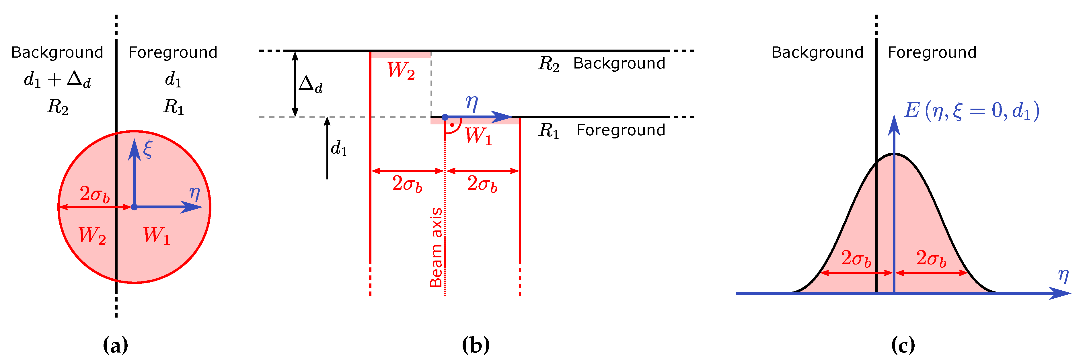
We assume an elliptical Gaussian measurement beam [24,29] illuminating simultaneously two perfectly planar and homogeneous targets parallel to each other and oriented normally to the beam axis. The transition between both targets is assumed to be a perfectly straight edge within the footprint dimensions. Figure 1 shows front (a) and top (b) view diagrams of this situation depicting both targets. The targets are defined by their respective spatially invariant reflectances and , and are placed at distances and from the instrument, respectively, where we assume that . The footprint partially covering both targets is also depicted in the figure, where is the horizontal beam radius (thus indicating the distance from the beam axis up to which, given a circular beam, 86% of the total power are contained [30,31]). and are respectively defined as the horizontal and vertical dimensions along the footprint on the front target. and , further explained below, represent the respective weights of the measurements corresponding to each target, defined by its reflectance and the portion of the beam illuminating it. The beam irradiance profile along at the front target distance is shown in Figure 1c.
While the figure represents a transition between targets along a vertical edge and the following derivations are therefore specified for the horizontal beam dimension , the analysis resulting therefrom is equally valid for the vertical dimension when the beam transits across a horizontal edge.
For distances much larger than the footprint diameter, as is the case for terrestrial laser scanning (with typical distances of several m or more, and typical beam diameters at the mm- to cm-level) except at close range and with extremely flat beam incidence, the distance variations within the footprint portion on each planar target can be neglected and the measurement process can be approximated as a weighted average of two single-point measurements where each reflecting surface is represented by a single distance. Considering the quasi-normal incidence on both targets, the distances can be approximated as and , respectively. The weights and , on the other hand, are proportional to the optical signal power received from foreground and background, respectively, where we may assume equal attenuation due to distance and atmosphere for both. The weights can thus be calculated as the integral of the irradiance over the respective portion of the footprint, scaled with the surface reflectance. Since we assumed that the separation between the targets is much smaller than the distance to the front target, the beam divergence between the targets can be neglected, and the integration can be carried out over the irradiance at the foreground distance, that is,
where is the location of the edge on the -axis.
As discussed in Section 2, the estimated distance is derived from the phase observation at the shortest modulation wavelength , and the ambiguity is resolved using larger wavelengths. Considering the derivation of the phase observation from the I- and Q-components, and their respective definition according to Equation (Section 2), the phase observation for the shortest wavelength is
The distance is then calculated from this phase according to Equation (2), where the number of full cycles is resolved from an additional measurement using a longer wavelength, as discussed in Section 2.
The impact of mixed pixels on phase-based LiDAR is twofold and depends in particular on the range of distances involved. If the separation between the targets is smaller than , the mixed pixel situation has no impact on the ambiguity resolution and only the phase of the smallest wavelength is affected. This case is modeled by Equation (8). The error introduced in this case results in a distance estimate somewhere between the true distances of both targets. Assuming a footprint that slides gradually across the edge, the distance changes smoothly between both true values and the distance error depends on the relative weights. When larger relative distances are involved, the ambiguity resolution algorithm yields different values for with the beam center in the vicinity of the edge, depending on the actual distances, on the measurement noise and on the relative weights. This introduces an apparent quantization and produces estimated distances only near integer multiples of in the region affected by mixed-pixels. When visualizing a point cloud this phenomenon appears as a set of equidistant, noisy replicas of the foreground contour towards the background. However, also in this case the resolution capability is affected by spatial averaging within the footprint and is fundamentally limited by the mixed pixel biases. This contribution to RC is therefore the focus of the model derived next.
Considering the foreground distance to be the true distance, the mixed-pixel bias for a specific edge between foreground and background (with specific reflectances and at specific distances) depends on the distance of the beam center from the edge. From a practical perspective, there will be no (significant) mixed-pixel bias if the beam center is far enough from the edge. We now aim at deriving an equation which predicts how close to the edge—or possibly even beyond it—the beam center can be such that the mixed-pixel bias is negligible. This will allow us to draw conclusions about the location and width of the regions around the target edges that are prone to significant errors. We define these errors as significant when they are larger than a threshold which we link to the expected noise level of the LiDAR sensor as .
Taking the front target as a reference and thus assuming that is the true distance, we determine the critical (minimum) ratio between the weights and for which the distance error exceeds the threshold:
The weights can be related to the beam properties by calculating the normalized power in the foreground target through integrating the Gaussian irradiance profile, defined by its shape parameter at , along the dimension perpendicular to the edge. This yields
where is the Gauss error function as resulting from integrating the probability density function of a normal distribution. Considering that the normalized power in the background is , we obtain
Plugging this and Equation (11) into (9), rearranging to express the position of the edge within the footprint, and denoting this particular position (where the ratio of and is exactly the critical ratio) , we obtain:
with being the inverse Gauss error function. Since there exists no closed form representation of this function, the above expression needs to be evaluated using a numerical approximation of .
From the perspective of the scanning process, this derivation provides a solution for calculating the critical distances around the edge of certain targets within which the impact of mixed pixels may become visible over the noise background. Results from the evaluation of this expression and a validation are presented and discussed in Section 5.1.
3.2. Resolution Capability
The mixed pixel model derived above can easily be extended to compute the width of the transition region between two targets where measurements cannot be resolved independently for one of the targets, thus indicating the resolution capability as limited by footprint spatial averaging. For this purpose, we need to complement the above by the critical value that conceptually corresponds to but denotes the position of the edge within the footprint where the mixed pixel bias first exceeds the threshold when moving the beam towards the edge from the background side and considering the background distance as the true distance. This edge position is obtained by replacing in Equation (13) with
The resolution capability can then be calculated as the width of the region between the limits and where measurements do not correspond reliably to any of the targets as
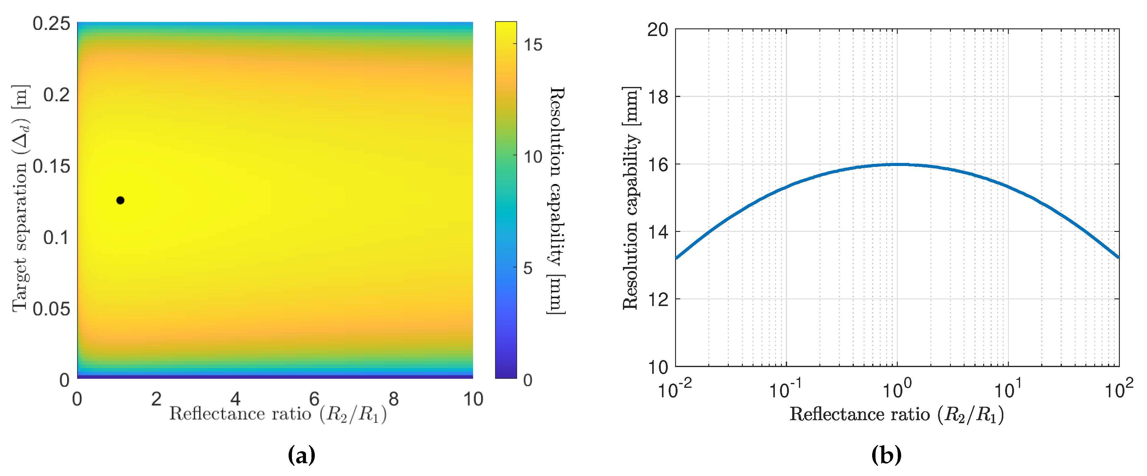
To analyze the impact of the separation and reflectances of foreground and background targets on , the derived resolution capability model has been computed for certain arbitrary but realistic instrument parameters. The resulting values for between 0 and , and reflectance ratios between 0.1 and 10 are depicted in Figure 2, where the absolute maximum (largest value of ) is indicated with a black dot. Equivalently to the mixed pixel biases, as modeled in Section 3.1, the resolution capability shows a periodicity of with the target separation . For such target separations the contributions of foreground and background to the overall phase at are almost in phase or in phase opposition and thus the mixed pixel situation primarily affects the total signal power while the distance measurement changes from foreground to background nearly suddenly as the beam sweeps across the edge. However, this situation is not practically relevant because of the impact of measurement noise. Furthermore, we restrict the RC analysis herein to small target separations, that is, , as mentioned above.
As can be seen in Figure 2a, the (practically relevant) maximum value of occurs at . Figure 2b shows as a function of the reflectance ratio for this particular target separation. This shows more clearly than Figure 2a that the resolution capability depends slightly on the ratio of the reflectances and is largest when .
Aiming at providing a simple expression that enables computing the resolution capability with little information on the scanner and scene properties, we have simplified the above model by only focusing on the worst case described above, that is, a target separation and equal reflectances () of the foreground and background planes. This results in
where is the inverse Gauss error function,
and the beam shape parameter at the measurement distance can be calculated from the nominal or measured beam parameters following the Gaussian beam model [22,23,24] as
with being the beam divergence half-angle, the beam waist radius, and the beam waist distance from the mechanical zero of the instrument.
Laser scanners typically realize the vertical beam deflection by means of a fast continuously rotating mirror. Additionally, phase-based LiDAR sensors internally accumulate the I and Q samples as of Equation (Section 2) over some time (integration time, herein) to collect enough signal power for a potentially high signal-to-noise ratio and thus high measurement precision. If the integration time during each measurement is not much smaller than the time between subsequent vertical measurements, the beam displacement during the integration introduces an effective elongation of the beam vertical dimension. The model can be extended to account for this effect when specifically calculating the vertical resolution capability by modifying the nominal beam parameters to calculate a specific vertical beam shape parameter . Approximating as the sum of the nominal beam shape parameter (corresponding to a static beam) and the apparent beam elongation resulting from the vertical displacement of the beam during the integration time (during which the beam constantly illuminates the surface but moves vertically), we obtain
where is the angular scanning resolution of the instrument as chosen by the user, represents the ratio between the measurement integration time and the time between subsequent measurement points ( would indicate integration across the complete transition between subsequent points), and the coefficient introduces the ratio between the beam shape parameter and the beam diameter. This extension is useful to provide a more realistic estimation of the vertical degradation of the resolution capability depending on the chosen scanning resolution and quality setting (longer integration time for higher quality). However, it requires to be estimated beforehand; the actual integration times for different scanner settings are usually not given in the specifications or manuals.
The simplified expressions in (16) to (19) provide a worst case estimation of the resolution capability that represents a useful indicator of the overall expected performance while only requiring knowledge of the distance to the targets of interest and the basic beam properties (divergence, waist radius and waist position), noise level and fine modulation wavelength of the instrument. Unlike beam properties and range noise, typically provided in the instruments’ specifications, the modulation wavelengths implemented in laser scanners are not usually disclosed by the manufacturers. Nevertheless, since range noise levels are in any case much smaller than the fine modulation wavelength, uncertainties in the value used for the above equations do not have a large impact on the computed resolution capability. For example, under realistic instrument parameters a deviation of 50% on the applied wavelength introduces deviations below 7% on the computed value of . In case no information at all is available regarding modulation wavelength, a value of 1 m is a reasonable choice considering current bandwidth limits in the hundreds of MHz range for commercially available modulators.
Aiming at providing an integral indicator of the expected resolution capability, the derived model for mixed-pixel limited resolution capability should be extended to account also for the influence of scanning resolution. Although the interplay between mixed pixels and scanning resolution may require a more specific investigation and is beyond the scope of this paper, we define a simple approximation for the total resolution capability by adding the angular scanning resolution such that
As opposed to Equation (19) which introduces an effective beam elongation only in the vertical direction (the integration time has virtually no influence on the horizontal beam shape), Equation (20) holds for both, horizontal and vertical RC. It takes into account that an object can only be resolved if it is wider than both the mixed-pixel zone and the distance between neighboring points in the point cloud.
4. Practical Approach for Mixed Pixel Analysis
In this section, we present the experimental measurement setup and the simulation framework used for the quantitative analysis of mixed pixel effects and for the validation of the equations derived above. Ideally, the experiments would yield measurements for different positions of the footprint center with respect to an edge and allow the footprint to be shifted in small increments from the beam being fully on the background to being fully on the foreground. This can be achieved easily with the numerical simulations (see Section 4.2). However, it is virtually impossible to achieve this movement of the footprint across an edge experimentally using a commercial terrestrial laser scanner which yields measurements at fixed, user-selected angular increments . We solve this problem in Section 4.1 by proposing a special target configuration for the scans.
4.1. Experimental Investigation
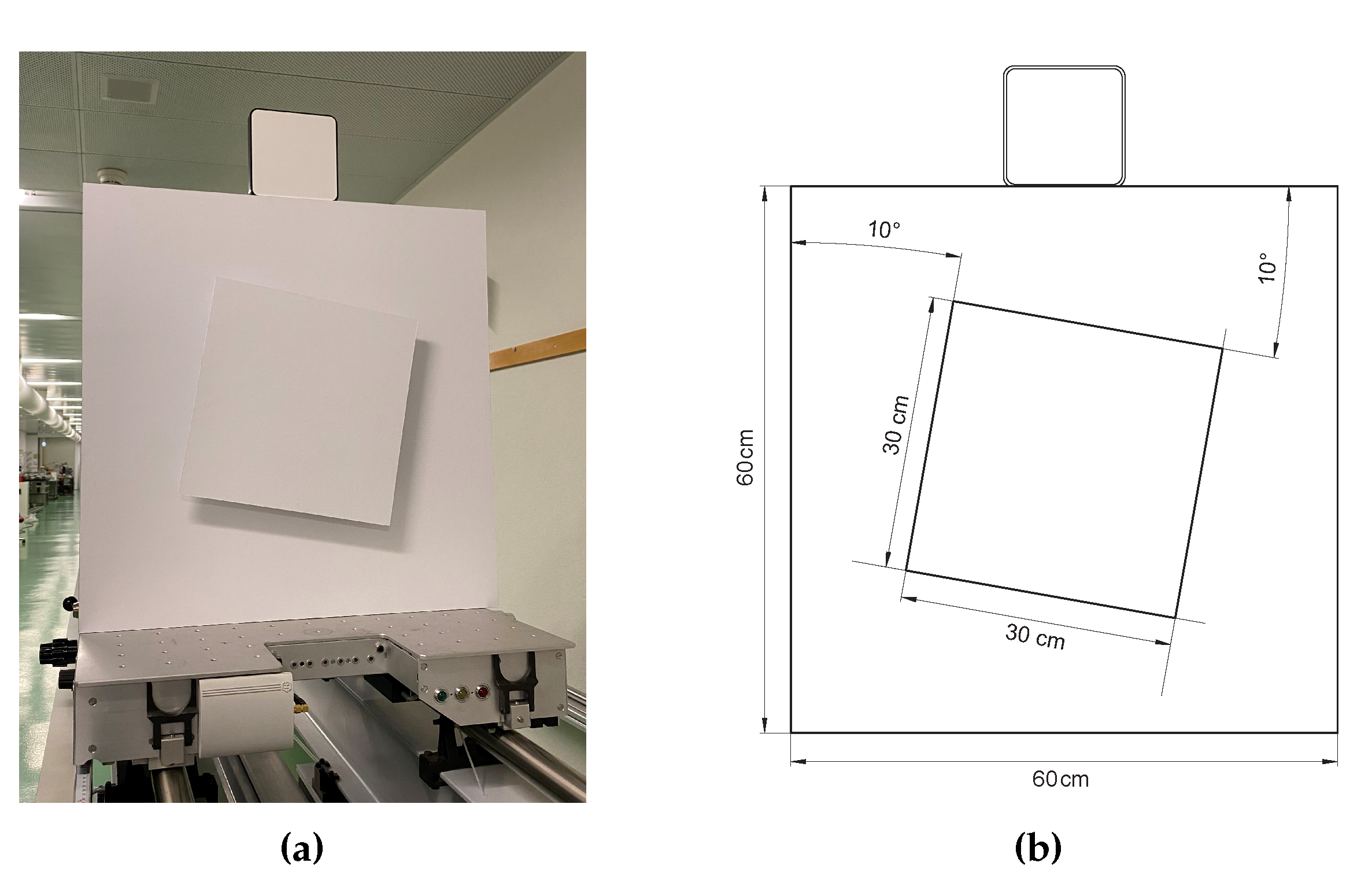
In order to obtain a sufficient number of mixed pixels and a large variety of relative footprint positions with respect to the edge from a normal scan, we use a square foreground plane which is slightly rotated such that neighboring points along vertical or horizontal profiles in the point cloud are associated with different footprint fractions on the foreground and background, see Figure 3 and explanations below. For practical reasons we have mounted the targets on a trolley which can be moved along a linear bench and enabled easily scanning the targets from different distances using a laser scanner set up at one end of the bench. The relative distance between the foreground and background planes can be changed manually between 3 and 23 cm. This range covers approximately the region where predicting the mixed pixel effects does not require assumptions regarding the ambiguity resolution algorithm (see Section 2). Additionally, we mounted a diffuse reflectance standard above the background target, see Figure 3, to enable estimation of the foreground and background reflectances from the scanner’s intensity data. Knowing the reflectances is not necessary for predicting the RC using our analytical model (see Equations (16) to (19)), but it allowed simulating exactly the real measurement situation later on. For all our own experiments reported herein, we used a Z&F Imager 5016 scanner, foreground and background plates with the same reflectance (73%), and a setup where the scanner is upright and approximately at the same height as the target center such that the beam hits the targets almost orthogonally across the entire target surface.
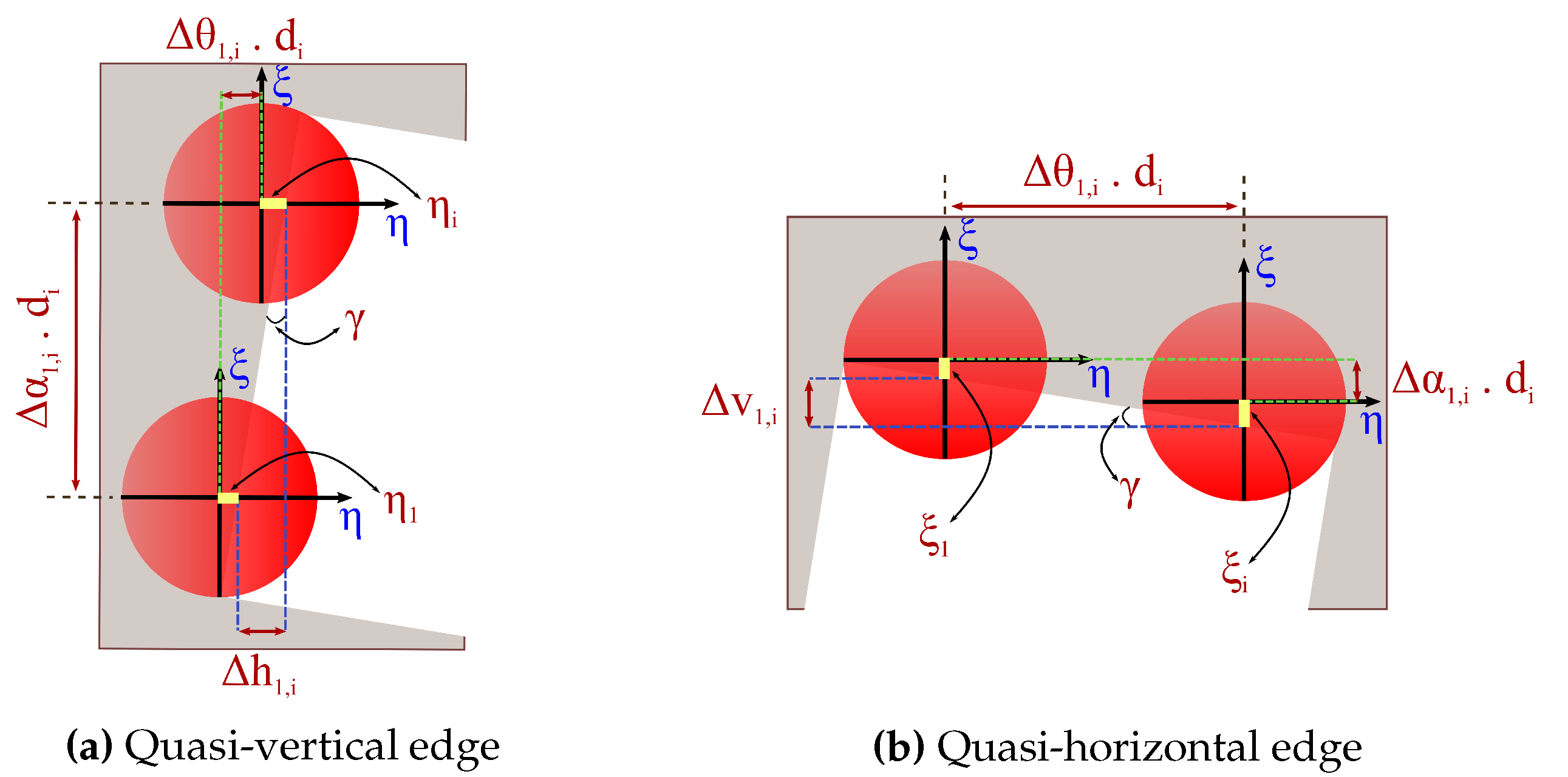
Analyzing the mixed pixel effects requires a quantification of the relative portion of the footprint on each of the targets. This is possible by calculating the differences and of the foreground-background edge position within the footprint (see Section 3.1 for the definition of and ) from the differences and of the polar coordinates of points in the point cloud. The relevant parameters of this transformation for the quasi-vertical and the quasi-horizontal edge are depicted in Figure 4.
The vertical movement of the footprint is depicted in Figure 4a which shows two points near the edge, one of which we arbitrarily picked from the point cloud as reference point for this analysis and denoted with the index 1, the other one arbitrarily assumed to be the ith picked point. and are the positions of the edge relative to the respective footprint center along the -axis. The relative change of the footprint center position with respect to the edge when moving from point 1 to point i is
where
is the shift resulting from the tilt angle between the edge and the scanner’s vertical axis, and are the differences of the horizontal and vertical angles of the two points, and is the 3d distance assumed to be approximately equal for both points, that is, . Except , all quantities can be extracted directly from the measured coordinates output by the scanner.
The transformation for the footprint displacement along the -axis (see Figure 4b) is achieved equivalently, where we assume the same tilt angle as above, now as the angle between the scanner’s horizontal axis and the edge:
with
These transformations are applied to the sections of the point clouds used for the mixed pixel analysis obtained from the experimental measurements. The transformed measurements enable representing the estimated distances uniquely as a function of the relative displacement of the footprint center with respect to the edge independently of the actual scanning process. Although still lacking information on the actual position of the edge—which is not known beforehand but will be derived from the measured points as part of the further analysis—the resulting data allows analyzing the mixed pixel effect as the footprint slides across the edge between foreground and background, see Section 5.1.
4.2. Numerical Simulation
The numerical simulation framework, presented in [27], refers to phase-based LiDAR measurements (Section 2). The simulations are extended to a 3D scanning process by deflecting the measurement beam at incremental angular directions. The simulations use a ray tracing approach to account for the energy distribution within the discretized laser footprint, surface geometry, and reflectivity of the surface material. The surfaces are geometrically represented as triangular irregular networks (TIN). The reflectivity properties are associated with the individual triangles via a Lambertian scattering model [32,33].
The simulation framework operates on a Gaussian irradiance beam profile [23,24] assumption, and allows to configure beam divergence, beam width and optical wavelength, as well as the set of modulation wavelengths used for the phase estimation. For the present paper, we use the framework to simulate measurements like the ones described in Section 4 but with a larger number of different configurations than in the real experiments. The beam parameters are taken from the specifications of the scanner used during the experimental investigation. The beam divergence is 0.3 mrad (half-angle), which corresponds to a beam waist radius of about 1.6 mm. The optical wavelength of the laser is 1500 nm, reported in [21,34]. There is no information about the implemented modulation wavelengths in the specifications. Judging from replicas produced in mixed pixel experiments with large separation between foreground and background, we assume that the shortest modulation wavelength is around 1.26 m and use this value herein. A longer modulation wavelength is only needed for ambiguity resolution. Since the impact of the latter is not investigated herein and we restrict to an analysis with short foreground-background separation where the ambiguity resolution does not affect the mixed pixel bias, the choice of the longer wavelength(s) is not critical. We arbitrarily chose , that is, 126 m, as the single longer modulation wavelength for the simulations.
5. Experimental Results
This section contains the mixed pixels analysis using the numerical simulation framework and the analytical model, in Section 5.1. Furthermore, in Section 5.2, it shows the experimental results of the beam parameter estimation of the Z&F Imager 5016 laser scanner using real measurements according to the procedure proposed in Section 4.1.
5.1. Mixed Pixels
We now study the mixed pixel effect numerically for a set-up equivalent to the one defined in Section 3. In particular, we use the numerical simulation framework with the beam parameters specified in Section 4.2 to predict the distances expected when measuring vertical profiles with negligibly small angular increments across a horizontal edge and we quantify how close to the edge the beam center can get at either side before the distance bias becomes significant. At this stage we assume a circular Gaussian beam. Therefore, the analysis of a horizontal measurement profile across a vertical edge would yield the same results.
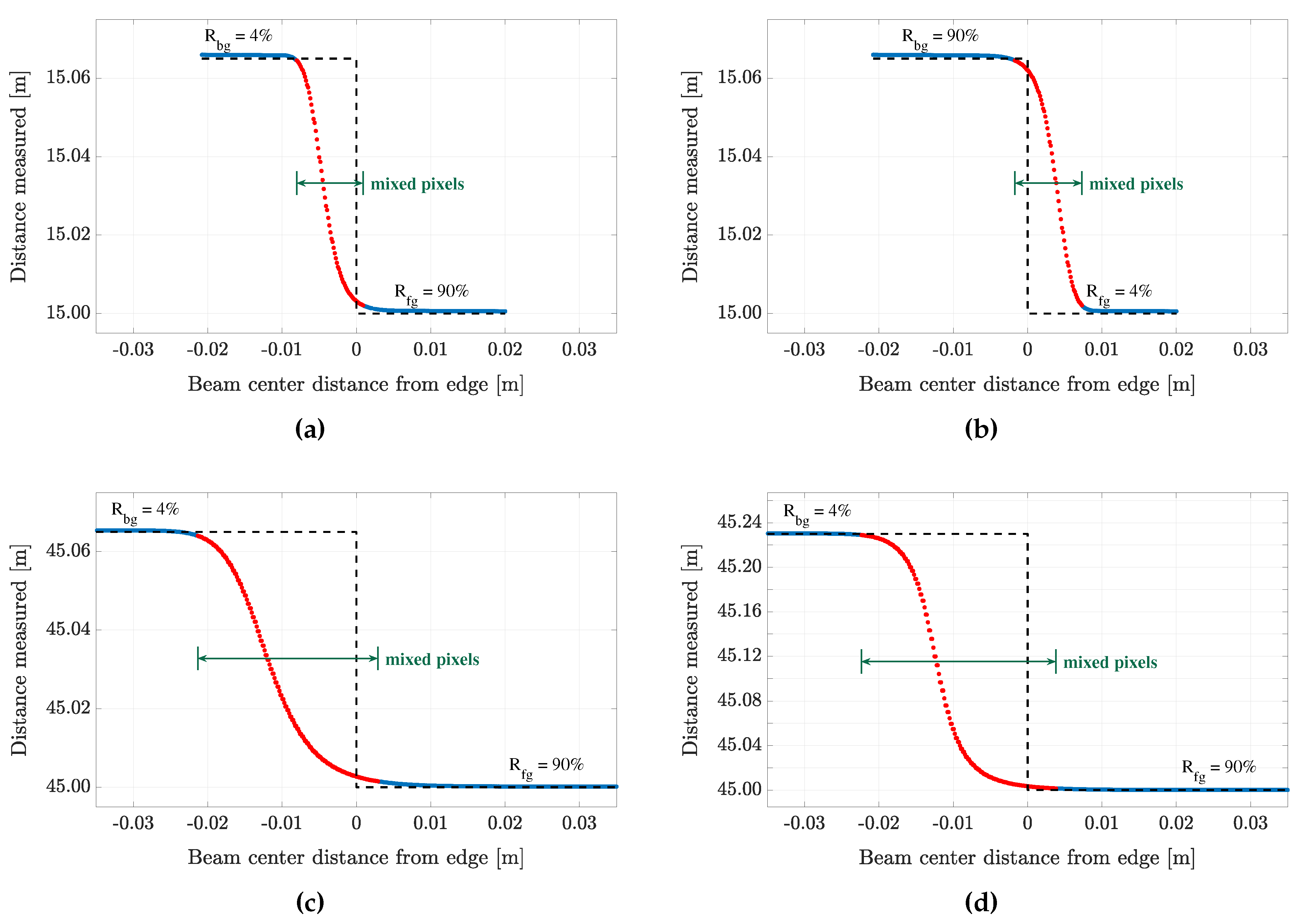
Figure 5 shows instructive examples of the results. The plots depict the estimated distance as a function of the footprint center position along the profile for certain combinations of parameters. The values significantly affected by mixed pixel biases are shown in red. They have been identified as those deviating from the geometrical distance along the beam center by more than . This threshold has been chosen for demonstration purposes only. Following the criteria given in Section 3, the threshold should be chosen smaller than the expected standard deviation of the distances in a real-world application.
Figure 5a shows a scenario with a bright foreground at 15 m and a dark background 6.5 cm farther away. The results were obtained using the beam parameters stated in Section 4.2. The beam divergence half-angle of 0.3 mrad results in a footprint diameter of 9.6 mm at this distance. When measurements are taken as the footprint moves across the background surface and transits beyond the edge of the foreground target, relevant errors occur if the beam center is closer than 8 mm to the edge. If instead the footprint approaches the edge from the foreground side significant errors occur only when the beam center is closer than 0.9 mm to the edge. So in this case the region around the edge affected by mixed pixels is about 8.9 mm wide (approximately corresponding to the footprint diameter), but it is not symmetric about the edge because of the large difference of foreground and background reflectances.
Actually, and in correspondence with the derivations given in Section 3.2, the numerical simulations showed that the width of the mixed pixel zone is practically independent of the reflectances, but the critical distances from the edge beyond which the bias is relevant, strongly depend on the ratio of the reflectances. This is corroborated by Figure 5b where the entire measurement setup is equal to the one of Figure 5a except the reflectances which are interchanged. The width of the affected zone is equal to the previous one (9 mm) but this zone now extends from 1.7 mm on the background side to 7.3 mm on the foreground side.
To see how this transition zone is affected by the distance, we also simulated scenarios with different distances. Figure 5c shows the results of such a calculation for a setup and beam parameters exactly as before (see Figure 5a) except the distance which is now 45 m to the foreground. As a consequence of the larger distance, the footprint diameter is also bigger (now approximately 27.2 mm). The width of the zone affected by mixed pixels is 24.2 mm wide, that is, scales roughly proportionally with distance and like the footprint although not exactly.
Figure 5d, corresponding to a scenario like the previous one but with an increased distance step between foreground and background (note different scaling of distance axis), finally shows that the impact of a larger relative distance between the two targets is comparably small; the transition zone is only slightly wider than before (26.2 mm), and the relative location of that zone about the edge does not change as compared to Figure 5c. Also these results are in agreement with the theoretical findings in Section 3.2.
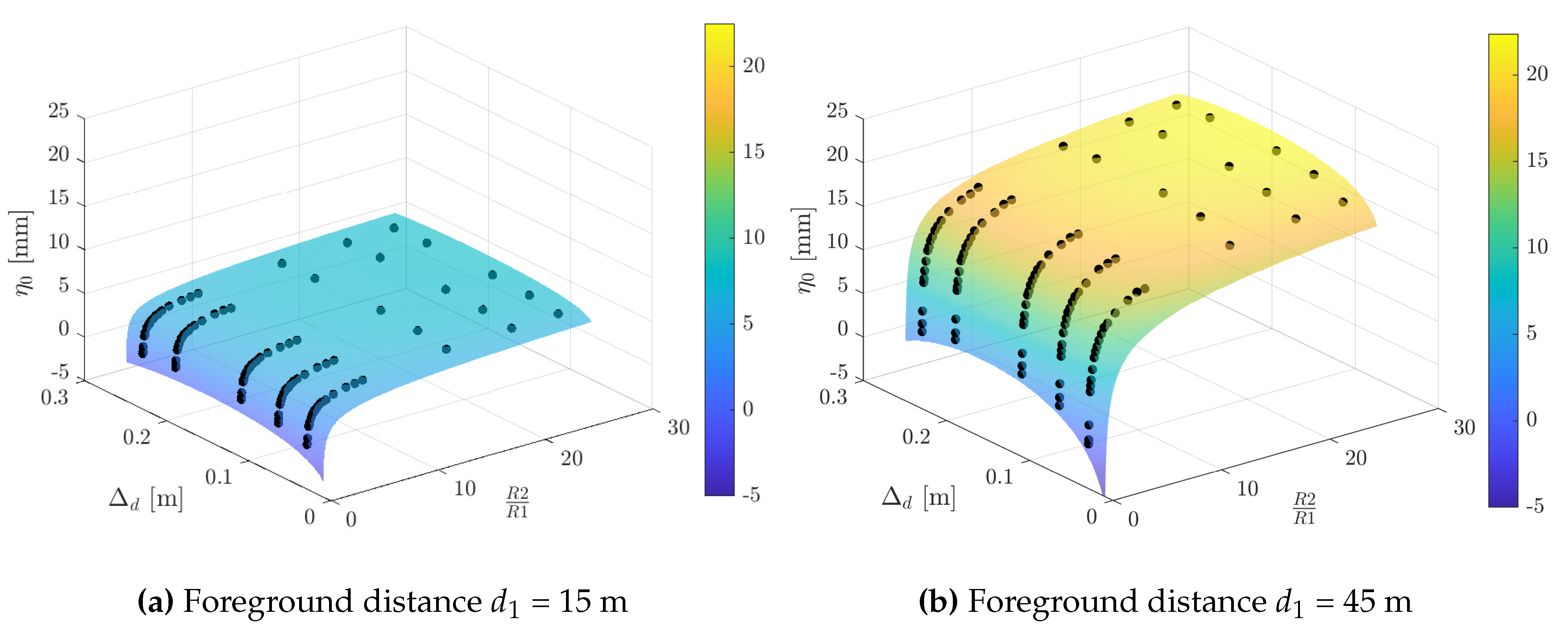
Using the numerical simulation of the measurement process, we have actually calculated the critical distances to the target edge for a variety of combinations of reflectances (4, 20, 50, 70 and 90%), distance steps (3, 6.5, 11, 19 and 23 cm), all lying within one quarter of , and for both distances (15 and 45 m). The results are shown as black dots in Figure 6. The semitransparent surfaces also shown in this figure were instead obtained for a dense grid of reflectances and distance steps using the analytical approximation Equation (13) derived in Section 3. The results agree at the sub-mm level which shows that the analytical approximation can be used to predict the critical distances and the width of the zone affected by mixed pixels.
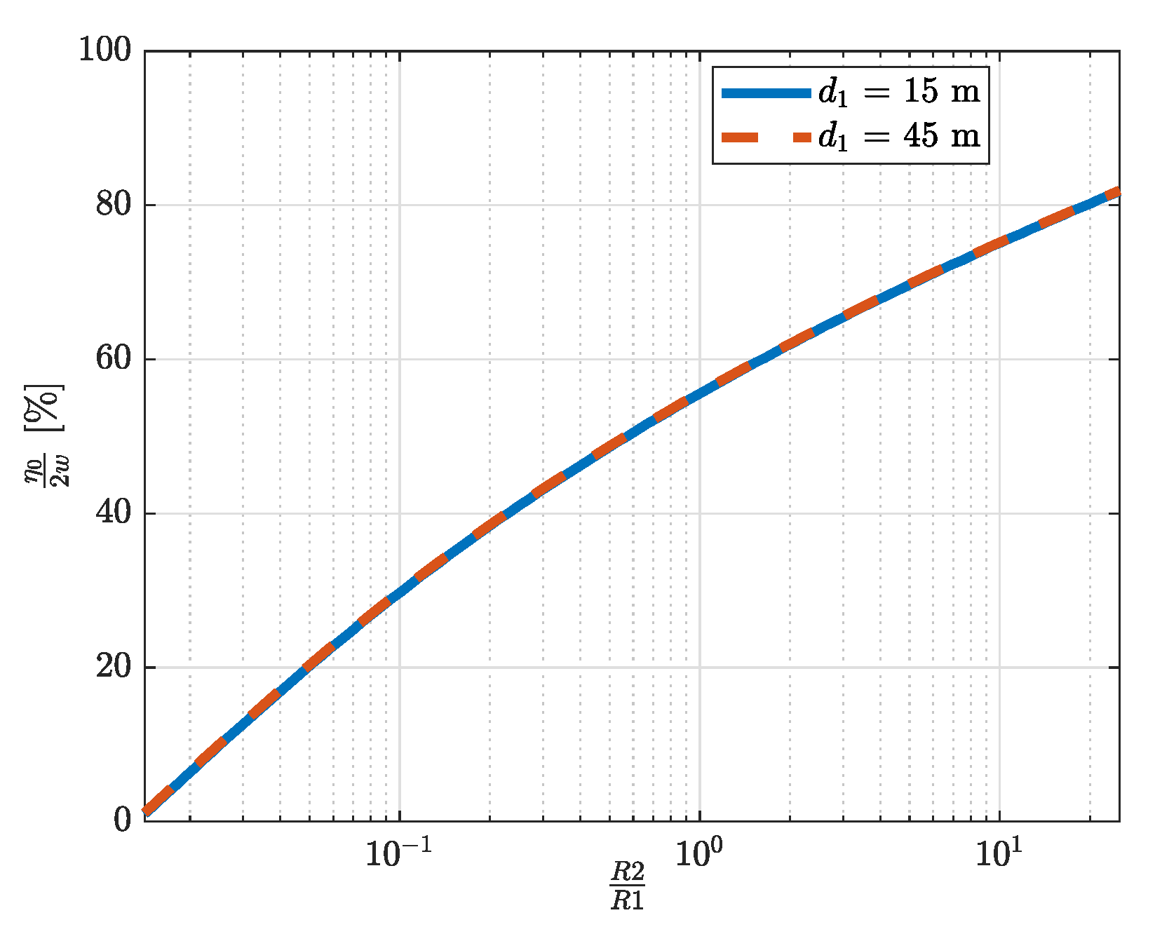
After this valdiation, we now use the analytical approximation to investigate the sensitivity of the mixed pixel effect further with respect to the reflectances and the relative distances. We already saw above that the errors are highly sensitive to the reflectance ratios and hardly sensitive to the separation between the surfaces. For closer inspection, the section of the surfaces in Figure 6 corresponding to is shown in slightly modified form in Figure 7. The critical distances are normalized to the respective beam diameter and the reflectance ratio is plotted on a logarithmic scale from about 0.01 to 30. While the values of seemed different for the 15 m and 45 m case before, they overlap almost perfectly in this display, thus indicating that, in the simple mixed pixel scenario depicted in Figure 1 and used to develop the analytical model, the critical value scales proportionally to the footprint. This overlap also holds for all other relative distances between 3 and 23 cm which we analyzed. Moreover, the dependence on the reflectance ratio suggests that when the foreground and background reflectances are equal, the critical distance is about 55% of the beam diameter and thus the width of the zone affected by mixed pixels is about 10% larger than the footprint.
5.2. Beam Parameter Estimation
The prediction of the mixed pixel effect and of the RC using the equations derived in Section 3 requires the beam shape parameter or equivalently the Gaussian beam radius w to be known. These quantities depend on the distance d and are related according to
We use the subscript x to indicate the dimension, that is, for the horizontal beam shape, and for the vertical one. According to the Gaussian model [22,24] the change of beam radius with distance is given by
The beam shape for arbitrary distances is thus known if the beam waist radius , the beam waist distance from the scanner, and the carrier wavelength of the modulated laser source are known. Except very close to the beam waist, the radius changes almost linearly with distance and the corresponding beam divergence half-angle is
If and cannot be extracted from the data sheet or from specifications given therein, an experimental setup like the one described in Section 4.1 may be used to derive these parameters experimentally. We describe the data processing and results obtained with a specific Z&F Imager 5016 laser scanner in this subsection.
We start by manually cutting out a part of the point cloud along the quasi-horizontal top edge of the foreground plate, see Figure 8 (blue points) for an example. This represents a band of vertical profiles from which we can estimate . Corresponding subsets of the point cloud are also selected for the other quasi-vertical or quasi-horizontal edges (see green points in Figure 8 for the left edge) to estimate also the horizontal beam shape and to check the results by independently deriving them from more than one edge. The areas cut-out should extend far enough beyond the edge to include also points which only represent the foreground or background and are not affected by mixed-pixel errors.
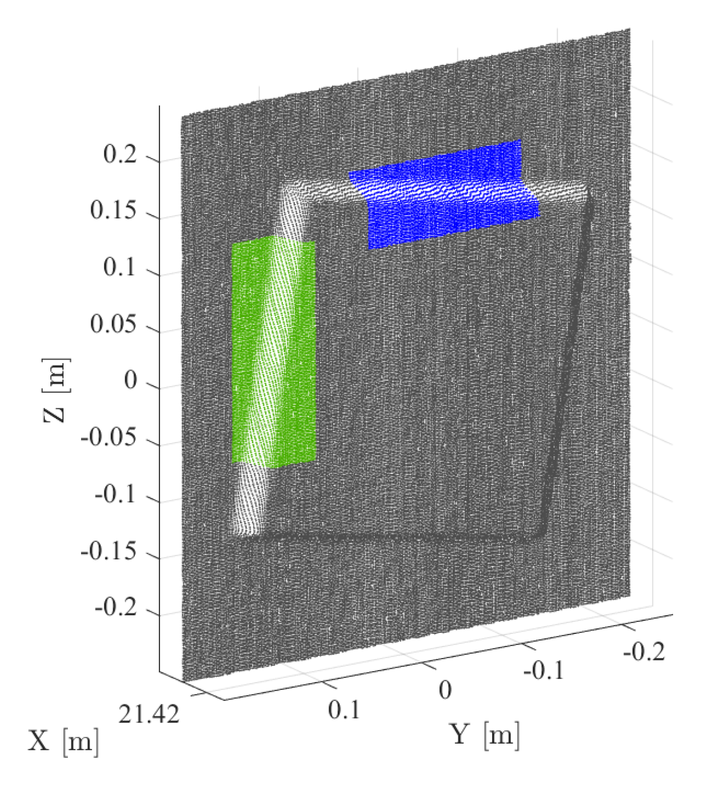
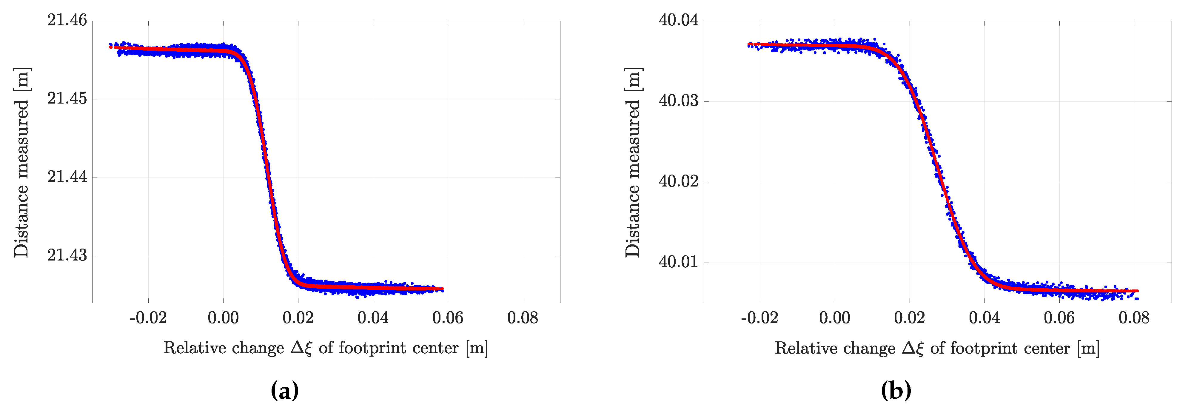
For the analysis, the angular coordinates of the beam centers (points in the cut-out subsets) are transformed into equivalent vertical edge coordinates , as introduced in Section 4.1, using Equation (23). One point in the selected band of profiles needs to be arbitrarily chosen as the origin of these transformed coordinates, that is, the point with index 1 in Equation (23). Herein, we pick the first point in the subset. Except for an initially unknown offset this transformation allows representing the measured distances as a function of the relative displacement of the footprint center with respect to the edge for a variety of coordinates. The result is displayed for the top edge and scans from two different distances in Figure 9 (blue dots).
If the true edge position, the true distances to foreground and background, the ratio of the reflectances, and the beam shape parameter were known, the experimental data as of Figure 9 would correspond to predicted data as of Figure 5 except for the impact of noise and of the approximations underlying our models. We can therefore estimate parameters within these models by adapting the assumed parameters such that the discrepancies between the transformed experimental data and the predictions are minimized in a suitable sense. Herein, we chose to estimate , , and from the data obtained across a quasi-horizontal edge using least-squares estimation (LSE). Equivalently, we preprocess point cloud data across a quasi-vertical edge and estimate , , and from those data. When using foreground and background of the same material and surface finish (see Section 4.1), : is known and does not need to be estimated. While it would be possible to jointly estimate all 4 parameters mentioned above from the data of all edges, we have decided to estimate them separately for each edge. This offers the opportunity to assess the quality of the estimated results by comparing them and it allows implicitly accounting for slightly non-parallel foreground and background edges without complicating the model.
The estimated beam radii obtained from scans with the highest quality setting (“premium”) and scanning resolution for different distances are given in Table 1. The corresponding distance predictions for two of the edges are shown as red dots in Figure 9; they visually confirm the successful representation of the data by the adapted model. The results reported in the table show a roughly linear dependence of beam radius on distance (as expected), agreement on the level of a few between corresponding edges (e.g., left and right), and slightly larger vertical than horizontal beam radius (including the apparent elongation due to data accumulation while the beam slides vertically along the surface). The formal standard deviations of the estimates as obtained from the LSE are below for close range and grow with distance to about for the case. The differences between the results obtained for corresponding edges, and later also the use of these values for estimating and (see below), suggest that these formal standard deviations are lower than the actual ones by a factor of about 8 to 10. This is likely due to data correlation ignored in the chosen LSE but is not a problem for the subsequent use of the estimated beam radii.
Given for different distances, Equation (25) can now be used to estimate the beam parameters and from which, in turn, the divergence half-angle and the beam radius for arbitrary distances can be calculated. We use the data from Table 1 for weighted LSE with weights inversely proportional to the squared formal standard deviations. The resulting estimates and their standard deviations are given in Table 2. The latter are based on the posterior variance factor and thus represent the actual misfit between the data from Table 1 and the model (25). Although it is theoretically possible to also estimate the optical wavelength of the measurement laser we have taken it as fixed herein, using the value reported for this scanner in [21,34]. Practically, w would need to be determined experimentally at several distances close to the beam waist in addition to larger distances, otherwise , and are highly correlated. However, the correlation is only problematic when comparing the estimated parameters to true ones or to values taken from the specification sheet, or when extrapolating the calculated beam radius to distances far from the ones covered by the samples. In the example given here, estimating the wavelength additionaly results in a (wrong) value of and different values also for and , but the calculated beam radii between 6 and differ by less than from the ones calculated using the results reported in Table 2. So, knowledge of is not critical for the present purpose. The beam parameters derived from scans in this way can be used to predict the RC for the respective scanner (see Section 6).
In view of Equation (19), the experimental determination of the beam parameters should be carried out with negligible beam elongation due to rotation of the laser beam (i.e., with a scanning resolution smaller than the beam divergence), because this beam elongation is modeled separately by the second term on the right hand side of (19). Nevertheless, the influence of various and different quality settings on the parameters of the effective footprint can be assessed using the approach outlined above when using scans obtained with different settings of the scanner. As an example of such a study, we show results (Table 3) of and obtained from scans at one particular distance only but for different scanning resolution and quality.
We see from these experimental investigations that the set by the user has an effect on the vertical footprint dimension whereas it has virtually no impact on the horizontal dimension. In correspondence with the simplified model introduced in Equation (19) larger vertical point spacing between consecutive measurements leads to an apparent vertical elongation of the beam. As opposed to that, the quality settings have no relevant impact on the beam parameters.
6. Results
Using a specifically designed target and the method presented in [15], an experimental evaluation of the resolution capability of several commercial scanners for different angular resolutions and quality levels has been given in [21]. We compare the vertical and horizontal resolution capability of the phase-based scanners (Leica HDS6100, Faro Focus X130 and Z&F Imager 5016) from that study to the results predicted using our model.
The beam and noise parameters used to evaluate our model for each scanner have been based on the manufacturer’s specifications. Some assumptions had to be made to derive these parameters despite insufficient or contradictory information in the specifications. Table 4 lists the parameters and reports the specific assumptions. The dependence of range noise on distance was interpolated from the given values using a quadratic polynomial. Additionally, the increase of range noise standard deviation in low-quality modes in relation to the specified values for high-quality modes was estimated assuming that it is inversely proportional to the square root of the measurement time (i.e., if the fastest scanning rate is m times the slowest (highest quality) one, noise is assumed to be times larger in the former).
The mixed-pixel threshold is defined as 2.58 times the range noise standard deviation, following the same criterion used experimentally in [15,21]. In the absence of any nominal information regarding the shortest modulation wavelength implemented on the assessed scanners, the value of 1.26 m assumed for the Z&F scanner from experimental results (see Section 4.2) and used in the mixed pixel analysis in Section 5.1 is taken as a sufficiently accurate assumption with little impact on the resolution capability results (see Section 3). The only instrument-related parameter that remains undefined and cannot be derived from the specifications or reasonably selected is the ratio between internal measurement accumulation time and scan time per point, as introduced in Equation (19). We have therefore computed the vertical RC for both extreme cases: indicating no beam elongation due to rotation of the beam, and , indicating measurements integrated across the whole transition between subsequent points, thus effectively elongating the vertical beam dimension to the complete point spacing.
The RC calculated from our model according to Equations (16) to (19) does not require any additional scenario-related parameter aside from the distance to the foreground target. As discussed in Section 3.2, the subsequent model results therefore refer to a worst—although still representative—case estimation corresponding to a target separation of ( = 15.75 cm) and equal reflectance of foreground and background ().
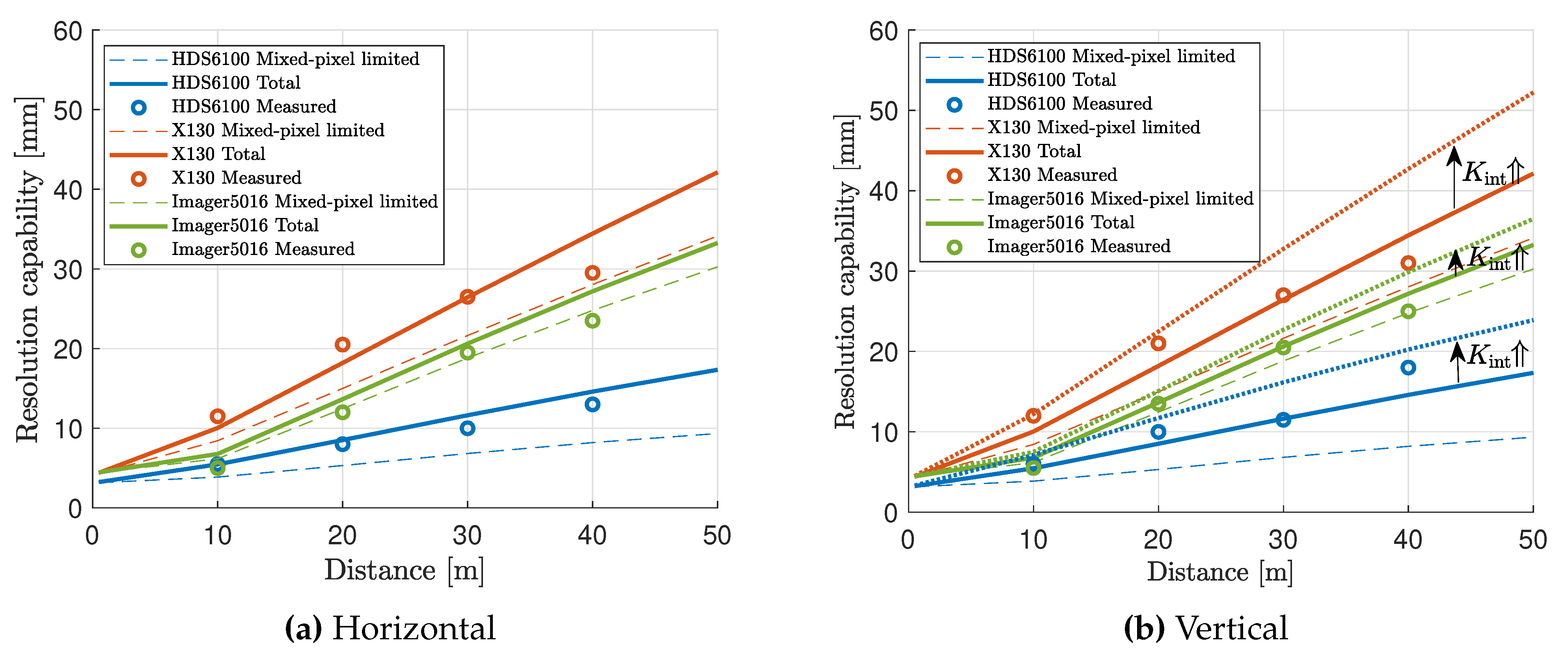
Figure 10 compares the resolution capabilities obtained experimentally in [21] (circles) and the ones computed with our model assuming the range noise level of the highest-quality mode and the highest scanning resolution. The model results are plotted separately for the mixed-pixel-limited contribution (dashed) and the total RC (solid) including the impact of the scanning resolution according to Equation (20). The vertical component in Figure 10 additionally shows the total RC (dotted) for the maximum vertical elongation () with the assumed scanning resolution. The simple numerical model is in very good agreement with the experimental results for all the scanners, in particular figuring in the standard deviations of the empirical results which are summarily reported as 0.1 to 3.7 mm in [15] and the fact that the experimental data have been extracted visually from plots given in [15,21].
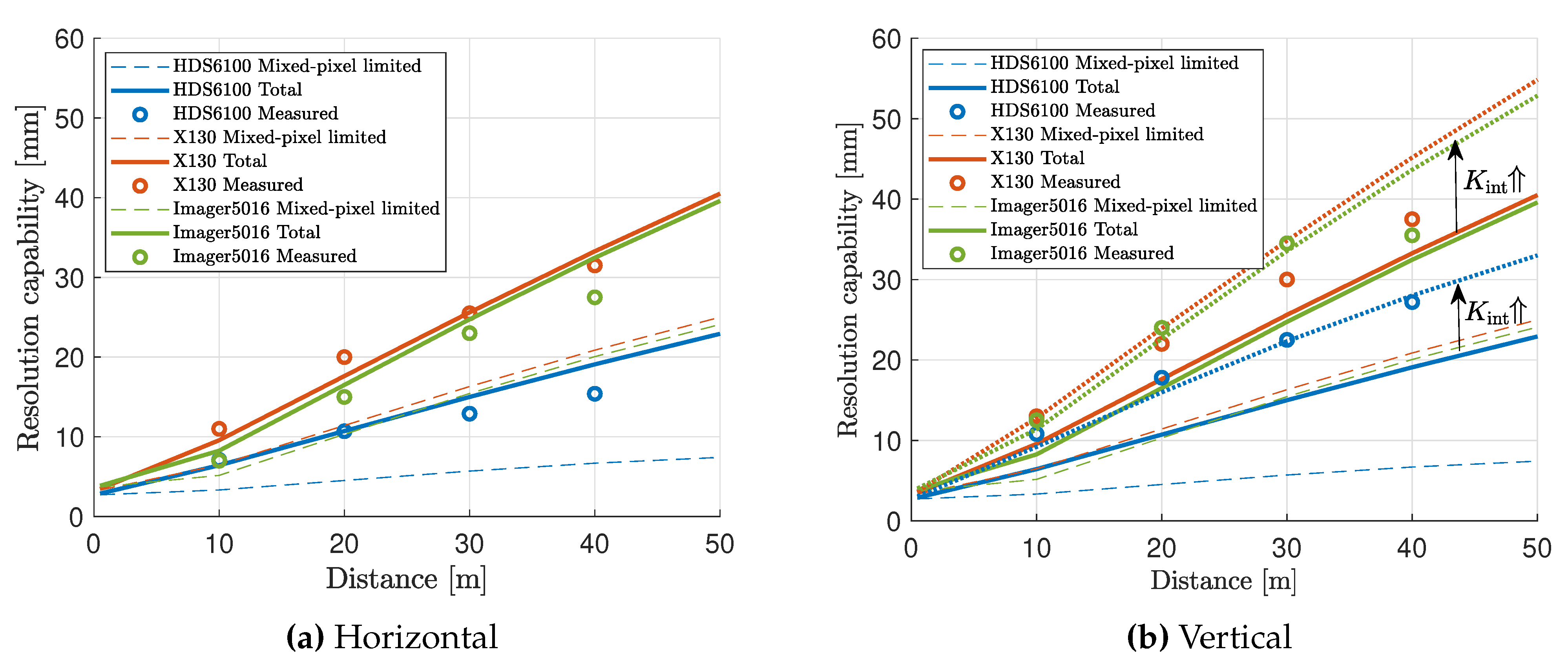
Figure 11 shows similar comparative results measured and computed for scanners set in low-quality mode and using a scanning resolution of 3.1 mm @ 10 m. Also in this case, the RC predicted by our simple model is in very good agreement with the experimental results.
There are multiple reasons that may explain the small deviations between model and experimental results. A slight overestimation of the RC can be generally expected from the model taking into account that it addresses a worst-case scenario regarding target-related parameters, and considering that the experimental method proposed in [15] computes the RC on measurements averaged across elongated sections of the point clouds, thus potentially underestimating the impact of scanning resolution due to randomization. Aside from these, the most plausible sources of deviations are a possibly more complex interplay between scanning resolution and mixed pixels in defining the total RC and, mostly, differences between the actual instrument parameters and the ones derived from the specifications—including assumptions when insufficient data was available—to compute the model. Among those, beam-related parameters are specially relevant due to the higher sensitivity of our model to them compared to the assumed range noise or modulation wavelength (e.g., an error of 50% in the assumed beam divergence introduces approximately the same relative error in the computed RC, whereas similar deviations in the range noise or modulation wavelength impact the RC by less than 10%).
The comparison between horizontal and vertical results for the lower scanning resolution—beam elongation is hardly significant for the highest scanning resolution—indicates that accounting for vertical elongation of the beam in fast scanning modes is relevant to estimate the RC more accurately, and that this impact is properly accounted for by our simple model. Information regarding the expected elongation, however, can be rarely derived from specifications and requires dedicated measurements as proposed in Section 4. The estimated beam parameters—including vertical elongation—derived experimentally for the Z&F scanner (see Table 2) indicate beam divergence values up to 30% larger than the one from the specifications. The RC predicted with our model using these estimated parameters is correspondingly larger. The results for the vertical component in low-resolution/low-quality mode (Figure 11b) provide a better agreement to the empirical results from [21] than if computed with the nominal values. These results are largely affected by vertical beam elongation, the higher agreement thus highlighting the advantage of using experimentally-obtained beam parameters in such situations. The results for all the other cases, however, show slightly worse agreement with the empirical results, likely caused by differences between the beam parameters of the specific instrument used in [21] and herein.
The agreement reached in the evaluated scanners indicates that the simple model proposed in this work can provide an estimation of the RC with sufficient accuracy for predicting the suitability of certain scanner, scanning configuration, and scanning resolution setting to meet measurement requirements regarding the effective resolution of the point cloud. Aside from the practical applicability of the proposed model, the observed agreement additionally shows the validity of the assumption discussed in Section 2 on the expected independence of RC with the implemented ambiguity resolution algorithm—unknown and possibly different among the investigated scanners—when the target separation is not much larger than a few dm. Furthermore, the results also corroborate that the actual measurement beams can be approximated as Gaussian beams.
7. Conclusions
We have developed an analytical expression for predicting and evaluating the resolution capability (RC) of phase-based laser scanners. This RC model represents the impact of spatial averaging over the footprint of the laser beam and includes the scanning resolution . We started by deriving a numerical model of the mixed pixel effect and using it to quantify how close to an edge a measurement beam center can be before a significant mixed-pixel bias is obtained. Therefrom we derived the width of the transition region next to an edge between two targets where the measurement no longer resolves one of the targets but instead represents a mixed pixel. The RC is the compound of this width and the scanning resolution.
We have validated the mixed pixel model using a numerical simulation framework of phase-based LiDAR and real scans with a Z&F Imager 5016 laser scanner. Finally, we have compared the RC predicted by our model to the RC empirically determined through laborious experiments by other authors. The excellent agreement indicates that our model can be used instead of the experiments for predicting the RC of a phase-based scanner with sufficient accuracy to decide whether the scanner and planned scanning configuration will yield point clouds with sufficient resolution for example, to represent the surfaces with the level of geometric details required by the intended application.
Both our mixed pixel and RC models are based on a Gaussian beam assumption and require certain beam parameters to be known, in particular beam waist radius and beam divergence. For the above comparison of our predictions to empirical results, we have assumed these values based on the specifications provided in the data sheets. However, in cases where the data sheets do not contain sufficient information or the parameters of a specific scanner’s beam should be compared to the specifications, it may be necessary to determine the parameters experimentally—possibly including the ellipticity. We thus also proposed a simple setup for a suitable experiment and the associated data processing herein.
Future extensions of the research will focus on further investigating the impact of the scanning resolution, and on covering also pulse-based scanners.
Author Contributions
Conceptualization, A.W.; methodology, S.C. and D.S.-M.; software and lab experiments, S.C.; analytical approximations, D.S.-M.; visualizations, S.C. and D.S.-M.; writing—original draft, S.C., D.S.-M. and A.W.; writing—review and editing, D.S.-M., A.W. and S.C.; supervision and funding acquisition, A.W. All authors have read and agreed to the published version of the manuscript.
Funding
This work was supported by the Swiss National Science Foundation (SNSF) under grant number 169318.
Institutional Review Board Statement
Not applicable.
Informed Consent Statement
Not applicable.
Data Availability Statement
The new data underlying this study are publicly available along with the MATLAB functions for calculating the beam parameters on GitHub: https://github.com/ChaudhrySukant/BeamProfiling.
Acknowledgments
Conflicts of Interest
The authors declare no conflict of interest.
References
- Lichti, D.D.; Gordon, S.J.; Tipdecho, T. Error Models and Propagation in Directly Georeferenced Terrestrial Laser Scanner Networks. J. Surv. Eng. 2005, 131, 135–142. [Google Scholar] [CrossRef]
- Kim, M.K.; Sohn, H.; Chang, C.C. Automated dimensional quality assessment of precast concrete panels using terrestrial laser scanning. Autom. Constr. 2014, 45, 163–177. [Google Scholar] [CrossRef]
- Wang, Q.; Kim, M.K.; Cheng, J.C.P.; Sohn, H. Automated quality assessment of precast concrete elements with geometry irregularities using terrestrial laser scanning. Autom. Constr. 2016, 68, 170–182. [Google Scholar] [CrossRef]
- Tang, P.; Akinci, B.; Huber, D. Quantification of edge loss of laser scanned data at spatial discontinuities. Autom. Constr. 2009, 18, 1070–1083. [Google Scholar] [CrossRef]
- Godbaz, J.P.; Dorrington, A.A.; Cree, M.J. Understanding and Ameliorating Mixed Pixels and Multipath Interference in AMCW Lidar. In TOF Range-Imaging Cameras; Springer: Berlin/Heidelberg, Germany, 2013; pp. 91–116. ISBN 978-3-642-27523-4. [Google Scholar]
- Hodge, R.A. Using simulated Terrestrial Laser Scanning to analyse errors in high-resolution scan data of irregular surfaces. ISPRS J. Photogramm. Remote Sens. 2010, 65, 227–240. [Google Scholar] [CrossRef]
- Olsen, M.J.; Kuester, F.; Chang, B.J.; Hutchinson, T.C. Terrestrial laser scanning-based structural damage assessment. J. Comput. Civ. Eng. 2010, 24, 264–272. [Google Scholar] [CrossRef]
- Hebert, M.; Krotkov, E. 3D measurements from imaging laser radars: How good are they? Image Vis. Comput. 1992, 10, 170–178. [Google Scholar] [CrossRef] [Green Version]
- Adams, M.D.; Probert, P.J. The Interpretation of Phase and Intensity Data from AMCW Light Detection Sensors for Reliable Ranging. Int. J. Robot. Res. 1996, 15, 441–458. [Google Scholar] [CrossRef]
- Tuley, J.; Vandapel, N.; Hebert, M. Analysis and Removal of Artifacts in 3-D LADAR Data. In Proceedings of the 2005 IEEE International Conference on Robotics and Automation, Barcelona, Spain, 18–22 April 2005; Volume 15, pp. 2203–2210. [Google Scholar]
- Tang, P.; Huber, D.; Akinci, B. A comparative analysis of depth-discontinuity and mixed-pixel detection algorithms. In Proceedings of the Sixth International Conference on 3-D Digital Imaging and Modeling (3DIM 2007), Montreal, QC, Canada, 21–23 August 2007; pp. 29–38. [Google Scholar]
- Wang, Q.; Sohn, H.; Cheng, J.C.P. Development of a mixed pixel filter for improved dimension estimation using AMCW laser scanner. ISPRS J. Photogramm. Remote Sens. 2016, 119, 246–258. [Google Scholar] [CrossRef]
- Wang, Q.; Sohn, H.; Cheng, J.C.P. Development of high-accuracy edge line estimation algorithms using terrestrial laser scanning. Autom. Constr. 2019, 101, 59–71. [Google Scholar] [CrossRef]
- Wang, Q.; Tan, Y.; Mei, Z. Computational methods of acquisition and processing of 3D point cloud data for construction applications. Arch. Comput. Methods Eng. 2020, 27, 479–499. [Google Scholar] [CrossRef]
- Schmitz, B.; Kuhlmann, H.; Holst, C. Investigating the resolution capability of terrestrial laser scanners and its impact on the effective number of measurements. ISPRS J. Photogramm. Remote Sens. 2020, 159, 41–52. [Google Scholar] [CrossRef]
- Lichti, D.D.; Jamtsho, S. Angular resolution of terrestrial laser scanners. Photogramm. Rec. 2006, 21, 141–160. [Google Scholar] [CrossRef]
- Boehler, W.; Vicent, M.B.; Marbs, A. Investigating laser scanner accuracy. Int. Arch. Photogramm. Remote Sens. Spat. Inf. Sci. 2003, 34, 696–701. [Google Scholar]
- Lichti, D.D. A resolution measure for terrestrial laser scanners. Int. Arch. Photogramm. Remote Sens. Spat. Inf. Sci. 2004, 34, B5. [Google Scholar]
- Pesci, A.; Teza, G.; Bonali, E. Terrestrial Laser Scanner Resolution: Numerical Simulations and Experiments on Spatial Sampling Optimization. Remote Sens. 2011, 3, 167–184. [Google Scholar] [CrossRef] [Green Version]
- Huxhagen, U.; Kern, F.; Siegrist, B. Untersuchung zum Auflösungsvermögen terrestrischer Laserscanner mittels Böhler-Stern. DGPF Tagungsband 2011, 20, 409–418. [Google Scholar]
- Schmitz, B.; Coopmann, D.; Kuhlmann, H.; Holst, C. Using the Resolution Capability and the Effective Num-ber of Measurements to Select the “Right” Terrestrial Laser Scanner. In Proceedings of the Contributions to International Conferences on Engineering Surveying, Dubrovnik, Croatia, 1–4 April 2020; pp. 92–104. [Google Scholar]
- Marshall, G.F. Gaussian laser beam diameters. In Laser Beam Scanning: Opto-Mechanical Devices, Systems, and Data Storage Optics; Marcel Dekker, Inc.: New York, NY, USA, 1985; pp. 289–301. [Google Scholar]
- Milonni, P.W.; Eberly, J.H. Laser Physics; John Wiley & Sons, Ltd.: Hoboken, NJ, USA, 2010. [Google Scholar]
- Saleh, B.; Teich, M. Fundamentals of Photonics, 3rd ed.; John Wiley & Sons: New York, NY, USA, 2019; ISBN 9781119506874. [Google Scholar]
- Rüeger, J.M. Electronic Distance Measurement: An Introduction; Springer Science & Business Media: Berlin, Germany, 2012. [Google Scholar]
- Proakis, J.G.; Salehi, M. Digital Communications, 5th ed.; McGraw Hill: New York, NY, USA, 2007. [Google Scholar]
- Chaudhry, S.; Salido-Monzú, D.; Wieser, A. Simulation of 3D laser scanning with phase-based EDM for the prediction of systematic deviations. In Proceedings of the International Society for Optics and Photonics (SPIE), Munich, Germany, 24–27 June 2019; Volume 11057, pp. 92–104. [Google Scholar]
- Braasch, M.S.; Van Dierendonck, A.J. GPS Receiver Architectures and Measurements. Proc. IEEE 1999, 87, 48–64. [Google Scholar] [CrossRef] [Green Version]
- Self, S.A. Focusing of spherical Gaussian beams. Appl. Opt. 1983, 22, 658–661. [Google Scholar] [CrossRef] [PubMed] [Green Version]
- Siegman, A.E.; Sasnett, M.W.; Johnston, T.F. Choice of clip levels for beam width measurements using knife-edge techniques. IEEE J. Quantum Electron. 1991, 27, 1098–1104. [Google Scholar] [CrossRef]
- Siegman, A.E. How to (maybe) measure laser beam quality. In Diode Pumped Solid State Lasers: Applications and Issues; DPSS: Washington, DC, USA, 1998; Volume 27, p. MQ1. [Google Scholar]
- Soudarissanane, S.S. The Geometry of Terrestrial Laser Scanning; Identification of Errors, Modeling and Mitigation of Scanning Geometry. Ph.D. Thesis, Technische Universiteit Delft, Delft, The Netherlands, 2016. [Google Scholar]
- Rees, W.G. Physical Principles of Remote Sensing; Scott Polar Research Institute: Cambridge, UK, 2001. [Google Scholar]
- Luhmann, T.; Robson, S.; Kyle, S.; Boehm, J. Close-Range Photogrammetry and 3D Imaging; De Gruyter: Berlin, Germany, 2020; ISBN 9783110607246. [Google Scholar]
Figure 1.
Modeled mixed pixel scenario with Gaussian footprint of horizontal radius covering a vertical transition between orthogonal planar foreground and background targets of reflectance and at distances and , respectively. (a) Front view, (b) top view, and (c) beam irradiance profile.
Figure 1.
Modeled mixed pixel scenario with Gaussian footprint of horizontal radius covering a vertical transition between orthogonal planar foreground and background targets of reflectance and at distances and , respectively. (a) Front view, (b) top view, and (c) beam irradiance profile.

Figure 2.
Resolution capability computed for a beam diameter ( of 12.8 mm, range noise and fine modulation wavelength : (a) as a function of target separation and reflectance ratio and, (b) as a function of reflectance ratio for fixed .
Figure 2.
Resolution capability computed for a beam diameter ( of 12.8 mm, range noise and fine modulation wavelength : (a) as a function of target separation and reflectance ratio and, (b) as a function of reflectance ratio for fixed .

Figure 3.
Target configuration of the experimental set-up. (a) Motorized trolley equipped with foreground plate, background plate and Spectralon reference target. (b) Dimensions and placing of the target components.
Figure 3.
Target configuration of the experimental set-up. (a) Motorized trolley equipped with foreground plate, background plate and Spectralon reference target. (b) Dimensions and placing of the target components.

Figure 4.
Parameters involved in the transformation between scanner coordinate system and footprint coordinate system.
Figure 4.
Parameters involved in the transformation between scanner coordinate system and footprint coordinate system.

Figure 5.
The transition width of the measurements (blue points) effected by the mixed pixels (red points) computed using the numeric simulation framework (Section 4.2) for different combinations of foreground and background reflectances [(a,c,d): = 90%, = 4%; (b): = 4%, = 90%], different foreground distances [(a,b): = 15 m; (c,d): = 45 m], and different relative distances [(a–c): = 6.5 cm; (d): = 23 cm].

Figure 6.
Critical distances calculated for a variety of configurations and the beam parameters stated in Section 4.2: numerical simulation (dots), analytical approximation (Equation (13)) (surfaces).
Figure 6.
Critical distances calculated for a variety of configurations and the beam parameters stated in Section 4.2: numerical simulation (dots), analytical approximation (Equation (13)) (surfaces).

Figure 7.
Critical distance , computed using the analytical approximation (Equation (13)), as a fraction of the footprint diameter and depending on the reflectance ratio .
Figure 7.
Critical distance , computed using the analytical approximation (Equation (13)), as a fraction of the footprint diameter and depending on the reflectance ratio .

Figure 8.
Point cloud obtained from a distance of 21.42 m, and subsets selected for beam parameter estimation from the top (blue) and left edge (green).
Figure 8.
Point cloud obtained from a distance of 21.42 m, and subsets selected for beam parameter estimation from the top (blue) and left edge (green).

Figure 9.
Measured points of top edge subset (blue) and corresponding model predictions (red) as a function of the footprint center position relative to the edge after beam parameter estimation for scans at about (a) 21 m and (b) 40 m. Both scans have been acquired with highest ( @ ) and with premium quality setting; refers to the arbitrary origin (see text), not to the actual position of the edge.

Figure 10.
Resolution capability as a function of distance on (a) horizontal and (b) vertical scanning directions for Leica HDS6100 (with scanning resolution 1.6 mm @ 10 m), Faro Focus X130 (with scanning resolution 1.6 mm @ 10 m) and Z&F Imager 5016 (with scanning resolution 0.8 mm @ 10 m). All instruments in high quality mode. Results of computation using our numerical approximation (dashed: mixed-pixel-limited, solid: mixed-pixel-limited + scanning-resolution-limited) and experimental results from real measurements on ad-hoc target as reported in [21] (circles).

Figure 11.
Resolution capability as a function of distance on (a) horizontal and (b) vertical scanning directions for Leica HDS6100 (results corrected with respect to [21] due to mislabeled dataset), Faro Focus X130 and Z&F Imager 5016. All instruments in low quality mode with scanning resolution 3.1 mm @ 10 m. Model computation (dashed: mixed-pixel-limited, solid: mixed-pixel-limited + scanning-resolution-limited) and real measurements on ad-hoc target from [21] (circles).


Table 1.
The experimentally determined horizontal beam radii along the left (←) and right (→) edges, and vertical beam radii along top (↑) and bottom (↓) edges for a Z&F Imager 5016 at various scanning distances with and premium (finest) quality setting.
Table 1.
The experimentally determined horizontal beam radii along the left (←) and right (→) edges, and vertical beam radii along top (↑) and bottom (↓) edges for a Z&F Imager 5016 at various scanning distances with and premium (finest) quality setting.
| Foreground Distance [m] | Beam Radius w [mm] | |||
|---|---|---|---|---|
| 6.0 | 1.8 | 2.0 | 1.9 | 2.1 |
| 21.4 | 7.0 | 7.0 | 7.7 | 7.7 |
| 25.0 | 8.2 | 8.2 | 9.0 | 9.2 |
| 40.0 | 13.3 | 13.7 | 15.4 | 14.9 |
| 51.8 | 17.3 | 17.3 | 20.1 | 19.8 |
Table 2.
Experimentally determined beam parameters for a Z&F Imager 5016 laser scanner at highest scanning resolution and quality.
Table 2.
Experimentally determined beam parameters for a Z&F Imager 5016 laser scanner at highest scanning resolution and quality.
| Dimension | Estimated Beam Waist | Estimated Beam Divergence | ||||
|---|---|---|---|---|---|---|
| Position | Radius | Half Angle | ||||
| [m] | [m] | [mm] | [mm] | [mrad] | [mrad] | |
| hz | 2.15 | 0.1 | 1.35 | 0.01 | 0.35 | 0.003 |
| vt | 1.93 | 0.1 | 1.22 | 0.02 | 0.39 | 0.006 |
Table 3.
The experimentally determined horizontal beam width radii along the left (←) and right (→) edges and vertical beam width radii along top (↑) and bottom (↓) edges for scans acquired at a distance of 21.42 m with different quality settings and scanning resolutions.
Table 3.
The experimentally determined horizontal beam width radii along the left (←) and right (→) edges and vertical beam width radii along top (↑) and bottom (↓) edges for scans acquired at a distance of 21.42 m with different quality settings and scanning resolutions.
| [mm @ 10 m] | Quality Setting | Beam Radius w [mm] | |||
|---|---|---|---|---|---|
| 0.8 | premium | 7.0 | 7.0 | 7.7 | 7.7 |
| 1.6 | premium | 7.1 | 7.0 | 9.3 | 9.3 |
| 3.2 | premium | 7.3 | 7.2 | 13.9 | 14.1 |
| 0.8 | high | 7.1 | 7.0 | 7.7 | 7.6 |
| 1.6 | high | 7.1 | 6.9 | 9.3 | 9.2 |
| 3.2 | high | 7.5 | 7.4 | 14.1 | 14.0 |
| 1.6 | normal | 7.1 | 7.0 | 9.3 | 9.3 |
| 3.2 | low | 7.1 | 7.3 | 13.9 | 13.8 |
Table 4.
Beam and noise parameters used for the resolution capability model computation of the evaluated scanners. : Beam size assumed to indicate diameter, as the most extended beam waist definition for laser scanners. : Beam waists assumed to be located at mechanical zero of instrument, being the most reasonable design choice in the absence of further specifications. : estimated from beam divergence and diameter at certain distance.
| Scanner | Beam Waist Radius [mm] | Beam Waist Position [m] | Divergence Half-Angle [mrad] | Range Noise Standard Deviation [mm] | |
|---|---|---|---|---|---|
| High-Quality | Low-Quality | ||||
| Leica HDS6100 | 1.5 | 0 | 0.11 | 0.72 @ 10 m 2.00 @ 50 m | 1.44 @ 10 m 4.00 @ 50 m |
| Faro Focus X130 | 1.6 | 0 | 0.27 | 0.26 @ 10 m 0.44 @ 50 m | 1.47 @ 10 m 2.51 @ 50 m |
| Z&F Imager 5016 | 1.6 | 3.43 | 0.3 | 0.14 @ 10 m 0.30 @ 50 m | 0.42 @ 10 m 0.85 @ 50 m |
Publisher’s Note: MDPI stays neutral with regard to jurisdictional claims in published maps and institutional affiliations. |
© 2021 by the authors. Licensee MDPI, Basel, Switzerland. This article is an open access article distributed under the terms and conditions of the Creative Commons Attribution (CC BY) license (http://creativecommons.org/licenses/by/4.0/).
Share and Cite
MDPI and ACS Style
Chaudhry, S.; Salido-Monzú, D.; Wieser, A. A Modeling Approach for Predicting the Resolution Capability in Terrestrial Laser Scanning. Remote Sens. 2021, 13, 615. https://0-doi-org.brum.beds.ac.uk/10.3390/rs13040615
AMA Style
Chaudhry S, Salido-Monzú D, Wieser A. A Modeling Approach for Predicting the Resolution Capability in Terrestrial Laser Scanning. Remote Sensing. 2021; 13(4):615. https://0-doi-org.brum.beds.ac.uk/10.3390/rs13040615
Chicago/Turabian StyleChaudhry, Sukant, David Salido-Monzú, and Andreas Wieser. 2021. "A Modeling Approach for Predicting the Resolution Capability in Terrestrial Laser Scanning" Remote Sensing 13, no. 4: 615. https://0-doi-org.brum.beds.ac.uk/10.3390/rs13040615
Note that from the first issue of 2016, this journal uses article numbers instead of page numbers. See further details here.