
Extracting the Tailings Ponds from High Spatial Resolution Remote Sensing Images by Integrating a Deep Learning-Based Model

 ,
,  and
and
Abstract
:
1. Introduction
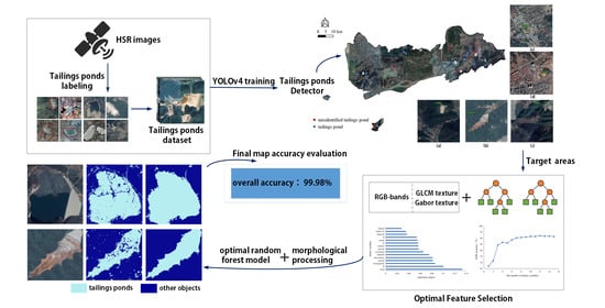
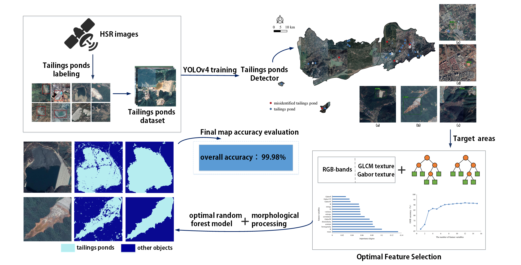
2. Methodology
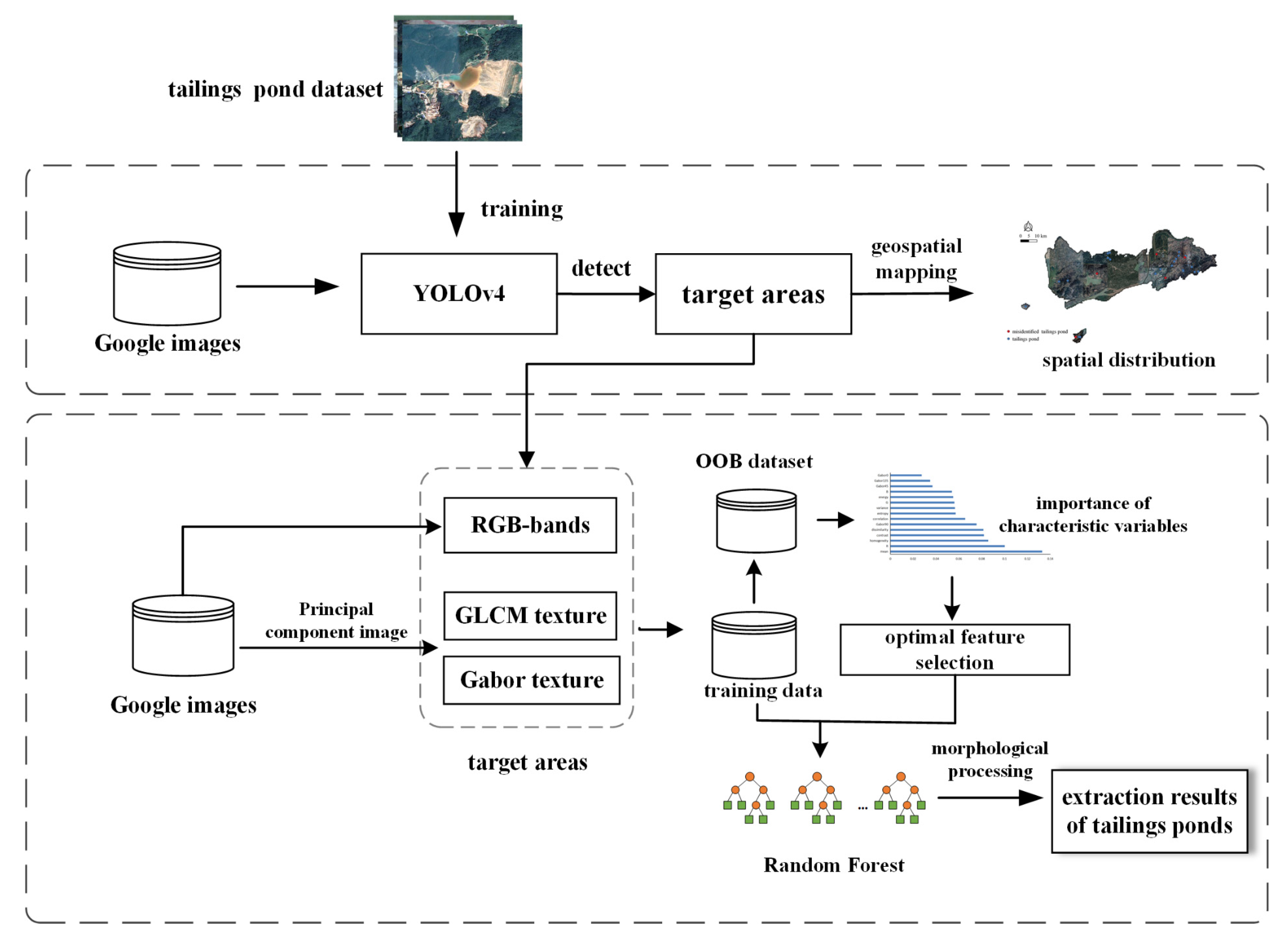
2.1. Detection of Tailings Pond Regions
2.2. Extraction of Tailings Ponds
2.2.1. Feature Extraction of Tailings Ponds
2.2.2. Random Forest Classification
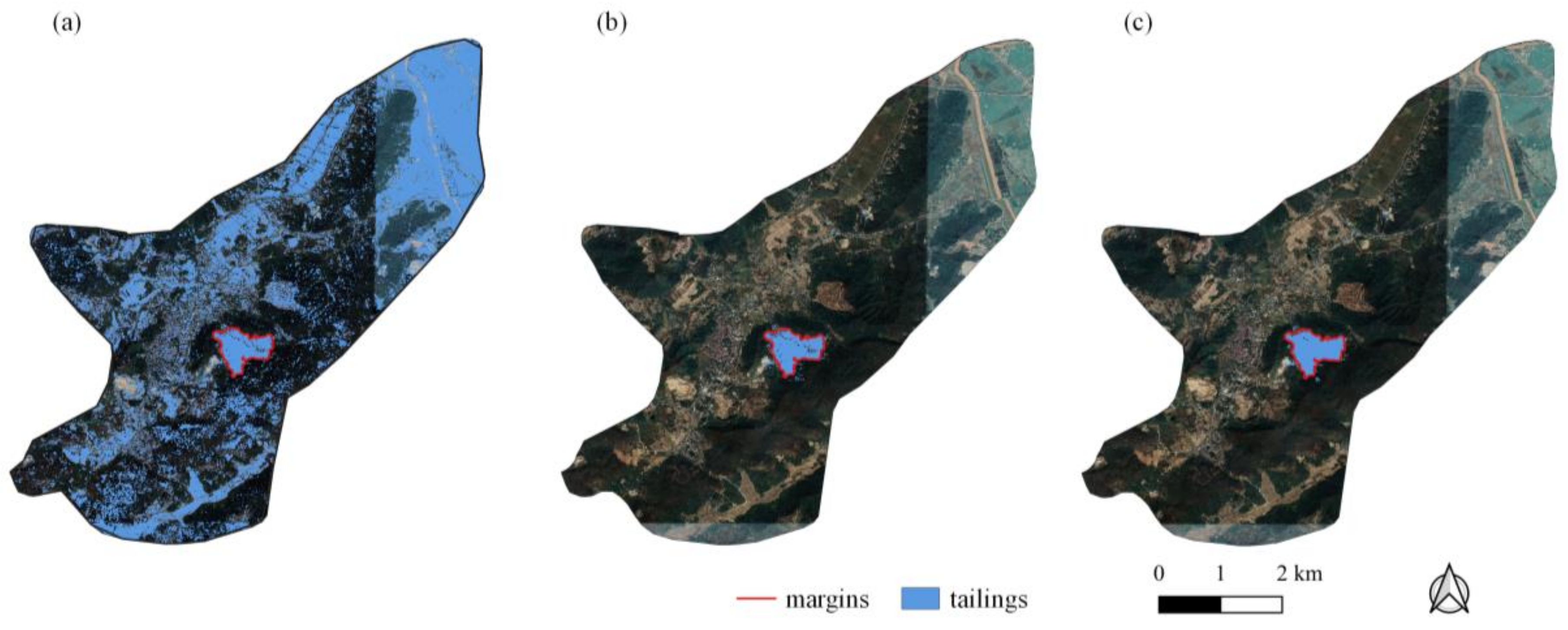
2.3. Morphological Processing
2.4. Accuracy Evaluation
2.4.1. Tailings Ponds Detection Accuracy Evaluation
2.4.2. Final Results Accuracy Evaluation
3. Results
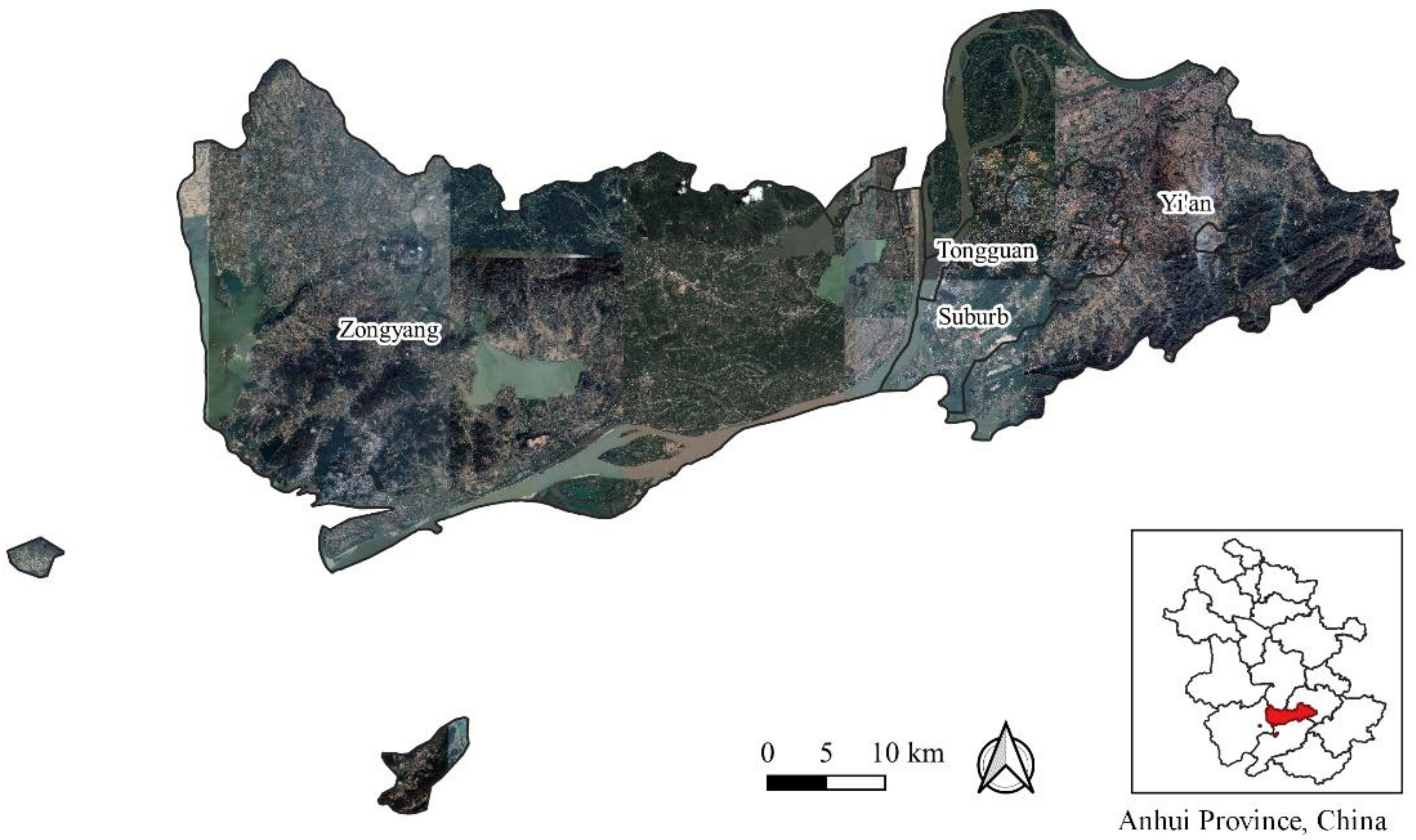
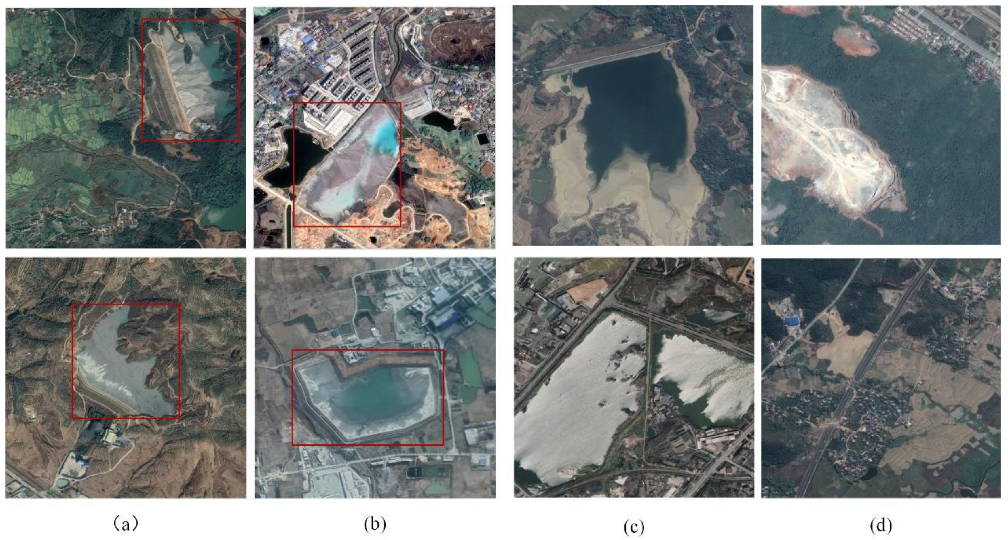
3.1. Study Area and Data
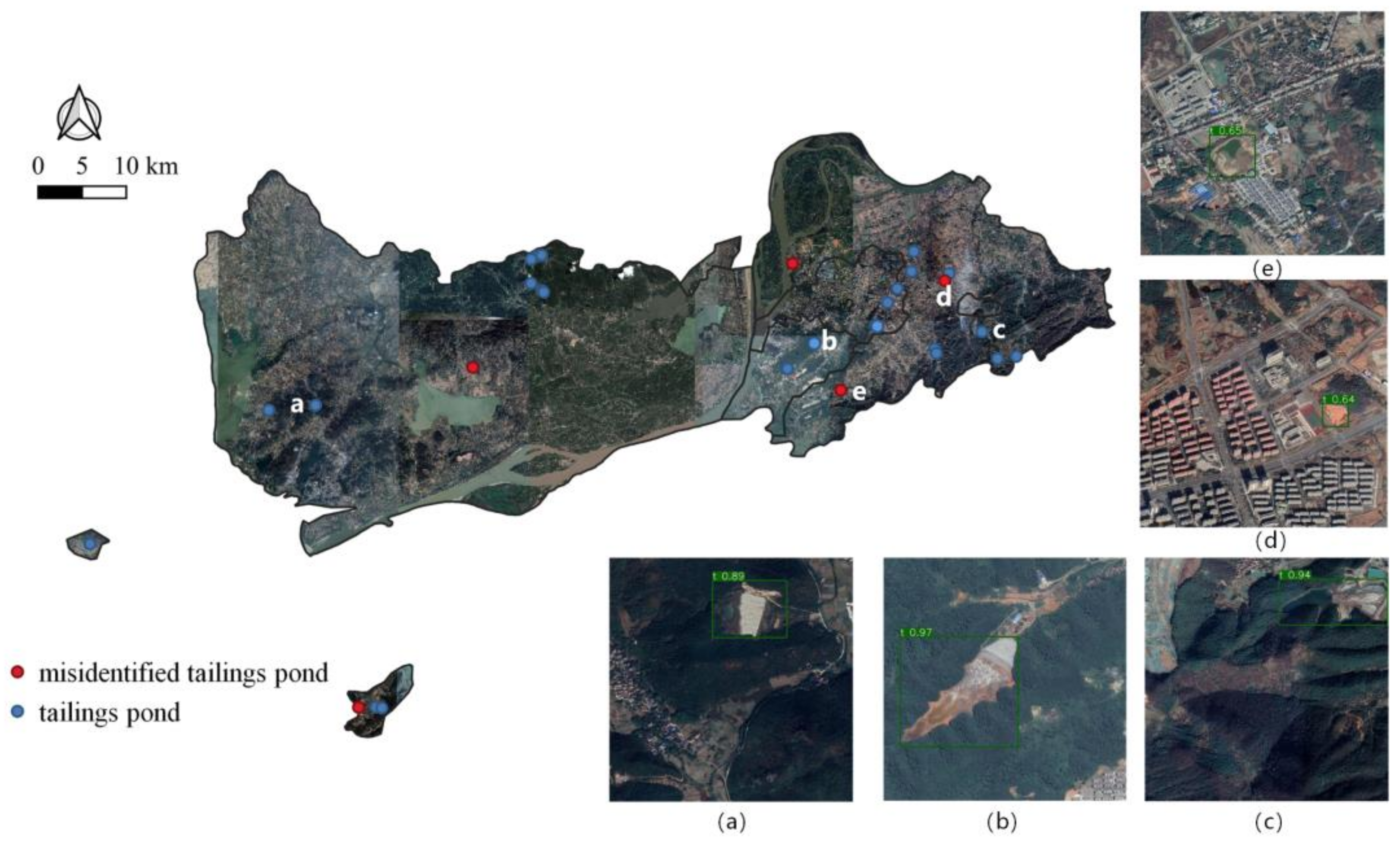
3.2. Detection of Tailings Ponds Based on YOLOv4
3.3. The Extraction of Tailings Ponds in Tongling
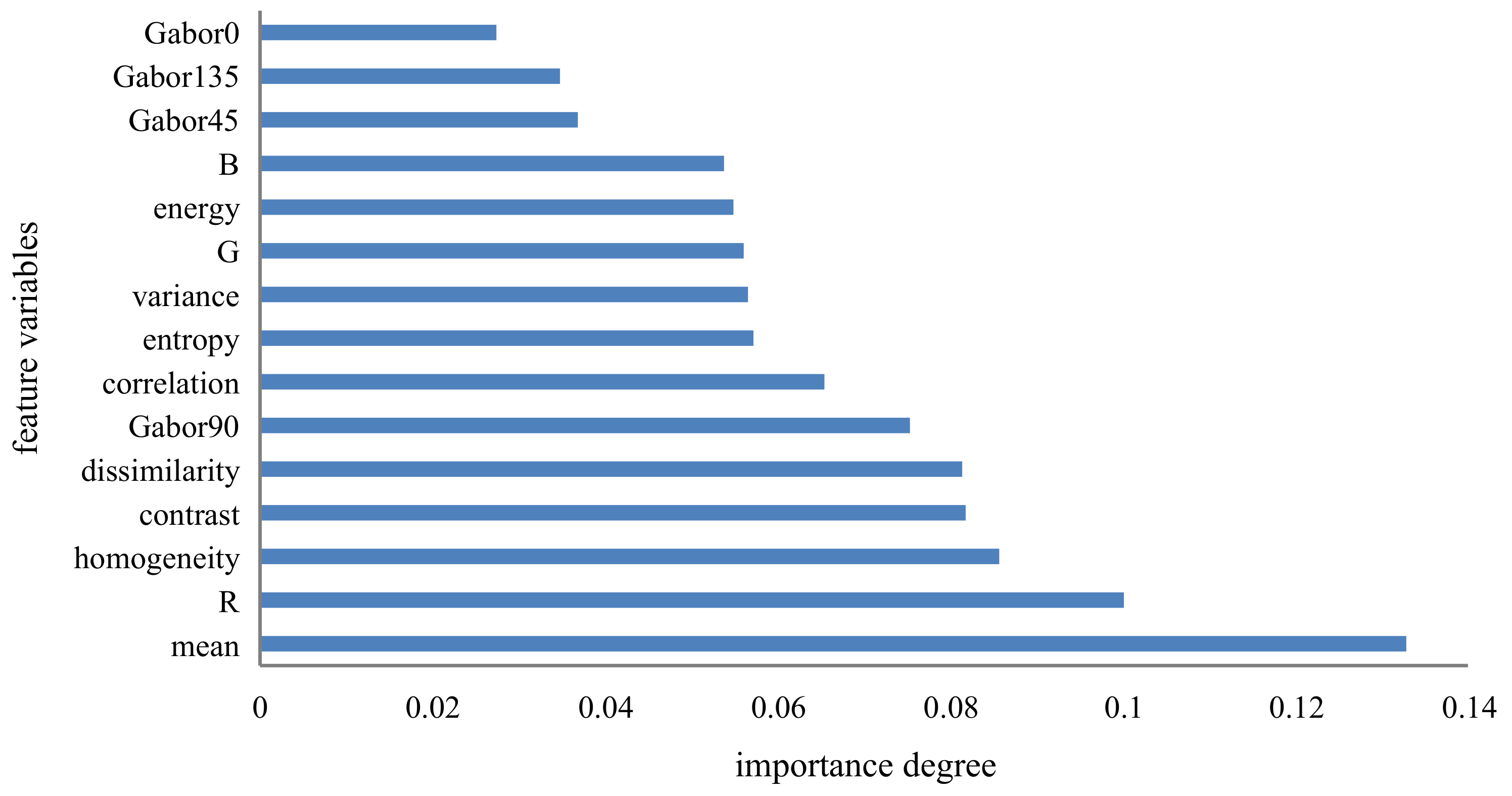
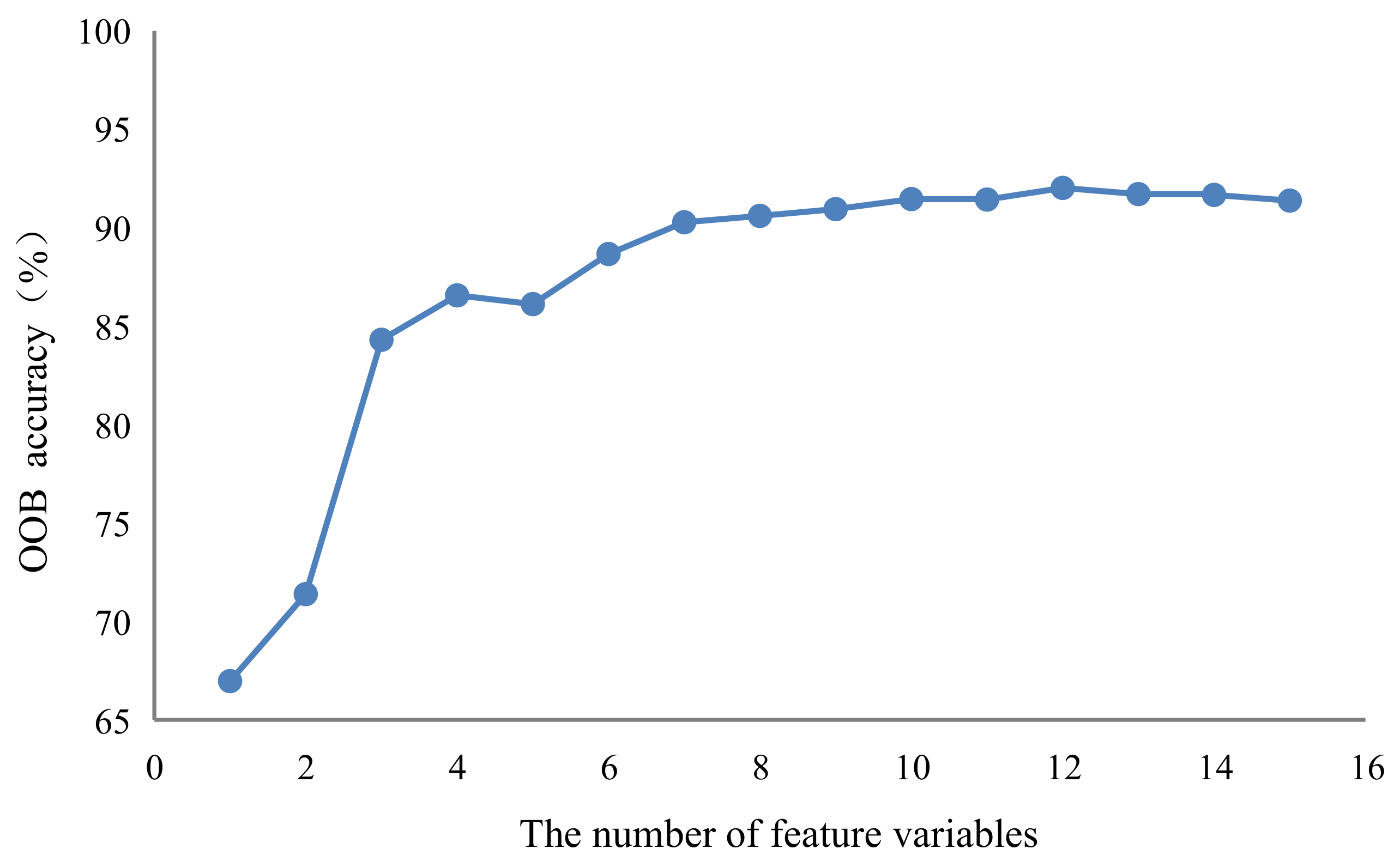
3.3.1. Selection of Optimal Features Based on Random Forest
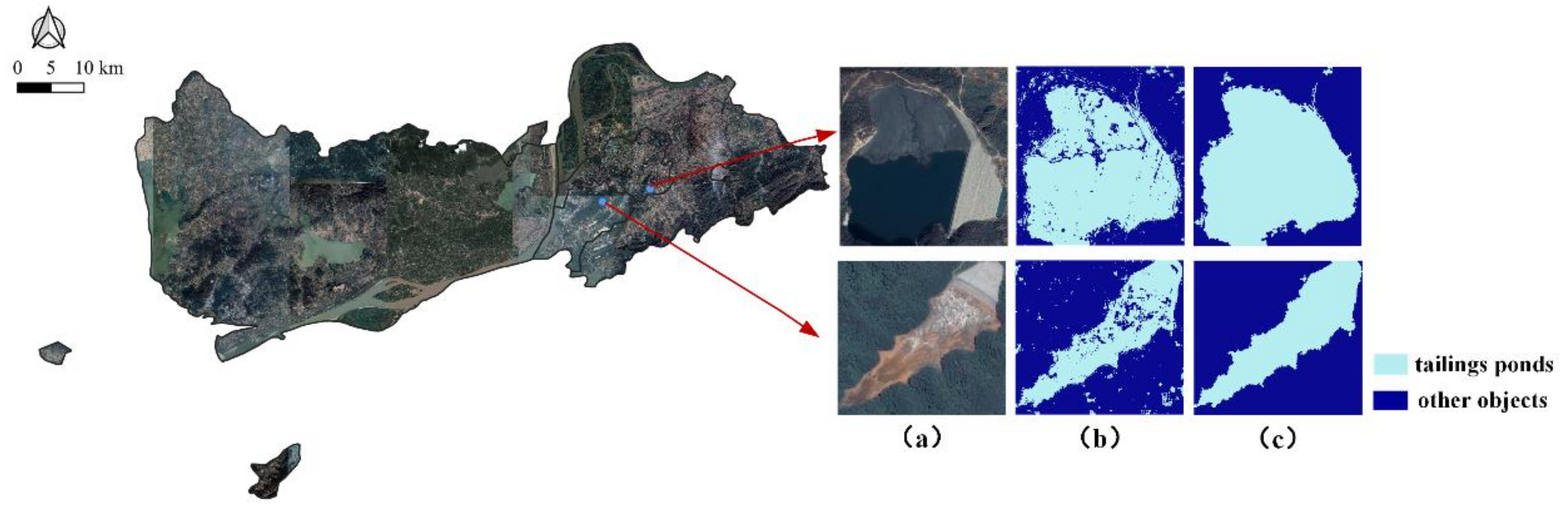
3.3.2. Extraction Results of Tailings Ponds
3.3.3. Final Map Accuracy Assessment
3.4. Model Comparison Results
4. Discussion
5. Conclusions
Author Contributions
Funding
Institutional Review Board Statement
Informed Consent Statement
Data Availability Statement
Acknowledgments
Conflicts of Interest
References
- BG, L. Mine Wastes: Characterization, Treatment and Environmental Impacts, 3rd ed.; Springer: Berlin/Heidelberg, Germany, 2010. [Google Scholar]
- Komnitsas, K.; Kontopoulos, A.; Lazar, I.; Cambridge, M. Risk assessment and proposed remedial actions in coastal tailings disposal sites in Romania. Miner. Eng. 1998, 11, 1179–1190. [Google Scholar] [CrossRef]
- Nasategay, F.F.U. Detection and Monitoring of Tailings Dam Surface Erosion Using UAV and Machine Learning; University of Nevada: Reno, NV, USA, 2020. [Google Scholar]
- Xiao, R.; Lv, J.; Fu, Z.; Wenming, S.; Wencheng, X.; Yuanli, S.; Fei, C.; Qianxiang, X. The application of remote sensing in the environmental risk monitoring of tailings pond in Zhangjiakou city, China. Remote Sens. Technol. Appl. 2014, 29, 100–105. [Google Scholar]
- Tang, L.; Liu, X.; Wang, X.; Liu, S.; Deng, H. Statistical analysis of tailings ponds in China. J. Geochem. Explor. 2020, 216, 106579. [Google Scholar] [CrossRef]
- Kossoff, D.; Dubbin, W.E.; Alfredsson, M.; Edwards, S.J.; Macklin, M.G.; Hudson-Edwards, K.A. Mine tailings dams: Characteristics, failure, environmental impacts and remediation. Appl. Geochem. 2014, 51, 229–245. [Google Scholar] [CrossRef] [Green Version]
- Mei, G. Quantitative assessment method study based on weakness theory of dam failure risks in tailings dam. Proc. Eng. 2011, 26, 1827–1834. [Google Scholar]
- Lyu, Z.; Chai, J.; Xu, Z.; Qin, Y.; Cao, J. A comprehensive review on reasons for tailings dam failures based on case history. Adv. Civil Eng. 2019, 9, 1–18. [Google Scholar] [CrossRef]
- Yu, D.; Tang, L.; Chen, C. Three-dimensional numerical simulation of mud flow from a tailings dam failure across complex terrain. Nat. Hazard. Earth Sys. 2020, 20, 727–741. [Google Scholar] [CrossRef] [Green Version]
- Zabcic, N.; Rivard, B.; Ong, C.; Müller, A. Using airborne hyperspectral data to characterize the surface pH and mineralogy of pyrite mine tailings. Int. J. Appl. Earth Obs. 2014, 32, 152–162. [Google Scholar] [CrossRef]
- Che, D.; Liang, A.; Li, X.; Ma, B. Remote sensing assessment of safety risk of iron tailings pond based on runoff coefficient. Sensors 2018, 18, 4373. [Google Scholar] [CrossRef] [Green Version]
- Lawley, V.; Lewis, M.; Clarke, K.; Ostendorf, B. Site-based and remote sensing methods for monitoring indicators of vegetation condition: An Australian review. Ecol. Indic. 2016, 60, 1273–1283. [Google Scholar] [CrossRef] [Green Version]
- Tan, Q.; Shao, Y. Application of remote sensing technology to environmental pollution monitoring. Remote Sens. Technol. Appl. 2012, 15, 246–251. [Google Scholar]
- Liu, K.; Liu, R.; Liu, Y. A Tailings Pond Identification Method Based on Spatial Combination of Objects. IEEE J. Sel. Top. Appl. Earth Observ. Remote Sens. 2019, 12, 2707–2717. [Google Scholar] [CrossRef]
- Schimmer, R. A remote sensing and GIS method for detecting land surface areas covered by copper mill tailings. In Proceedings of the Pecora, Denver, CO, USA, 18–20 November 2008. [Google Scholar]
- Ma, B.; Yuteng, C.; Song, Z.; Xuexin, L. Remote Sensing Extraction Method of Tailings Ponds in Ultra-Low-Grade Iron Mining Area Based on Spectral Characteristics and Texture Entropy. Entropy 2018, 20, 345. [Google Scholar] [CrossRef] [Green Version]
- Hao, L.; Zhang, Z.; Yang, X. Mine tailing extraction indexes and model using remote-sensing images in southeast Hubei Province. Environ. Earth Sci. 2019, 78, 493. [Google Scholar] [CrossRef] [Green Version]
- Zhang, X.; Xiao, P.; Feng, X.; Yuan, M. Separate segmentation of multi-temporal high-resolution remote sensing images for object-based change detection in urban area. Remote Sens. Environ. 2017, 201, 243–255. [Google Scholar] [CrossRef]
- Hao, L.; Zhang, Z.; He, W.X.; Chen, T. Tailings reservoir recognition factors of the high resolution remote sensing image in Southeastern Hubei. Remote Sens. Land Resour. 2012, 24, 154–158. [Google Scholar]
- Gao, Y.; Chu, Y.; Liang, W. Remote sensing monitoring and analysis of tailings ponds in the ore concentration area of Heilongjiang Province. Remote Sens. Land Resour. 2015, 27, 160–163. [Google Scholar]
- Zhou, Y.; Wang, X.; Yao, W.; Yang, J. Remote sensing investigation and environment impact analysis of tailing ponds in Shandong province. Geol. Surv. China 2017, 4, 88–92. [Google Scholar]
- Mezned, N.; Mechrgui, N.; Abdeljaouad, S. Mine wastes environmental impact mapping using Landsat ETM+ and SPOT 5 data fusion in the North of Tunisia. J. Indian Soc. Remote 2016, 44, 451–455. [Google Scholar] [CrossRef]
- Li, Q.M.; Zhang, H.; Li, G. Comparative analysis on safety management of tailings ponds in China and Canada. China Min. Mag. 2017, 26, 21–24. [Google Scholar]
- Kussul, N.; Lavreniuk, M.; Skakun, S.; Shelestov, A. Deep learning classification of land cover and crop types using remote sensing data. IEEE Geosci. Remote Sens. 2017, 14, 778–782. [Google Scholar] [CrossRef]
- Zhang, L.; Xia, G.; Wu, T.; Lin, L.; Tai, X.C. Deep learning for remote sensing image understanding. J. Sens. 2016, 501, 173691. [Google Scholar] [CrossRef]
- Ball, J.E.; Anderson, D.T.; Chan, C.S. Comprehensive survey of deep learning in remote sensing: Theories, tools and challenges for the community. J. Appl. Remote Sens. 2017, 11, 42609. [Google Scholar] [CrossRef] [Green Version]
- Zou, Q.; Ni, L.; Zhang, T.; Wang, Q. Deep learning based feature selection for remote sensing scene classification. IEEE Geosci. Remote Sens. 2015, 12, 2321–2325. [Google Scholar] [CrossRef]
- Alshehhi, R.; Marpu, P.R.; Woon, W.L.; Mura, M.D. Simultaneous extraction of roads and buildings in remote sensing imagery with convolutional neural networks. ISPRS J. Photogramm. Remote Sens. 2017, 130, 139–149. [Google Scholar] [CrossRef]
- Cao, Y.; Niu, X.; Dou, Y. Region-based convolutional neural networks for object detection in very high resolution remote sensing images. In Proceedings of the 12th International Conference on Natural Computation, Fuzzy Systems and Knowledge Discovery (ICNC-FSKD), Changsha, China, 13–15 August 2016. [Google Scholar]
- Ren, S.; He, K.; Girshick, R.; Sun, J. Faster r-cnn: Towards real-time object detection with region proposal networks. In Proceedings of the Advances in Neural Information Processing Systems, Montreal, QC, Canada, 7–12 December 2015. [Google Scholar]
- Liu, W.; Anguelov, D.; Erhan, D.; Szegedy, C.; Reed, S.; Fu, C.; Berg, A.C. Ssd: Single shot multibox detector. In Proceedings of the 14th European Conference on Computer Vision, Amsterdam, The Netherlands, 8–16 October 2016. [Google Scholar]
- Redmon, J.; Divvala, S.; Girshick, R.; Farhadi, A. You only look once: Unified, real-time object detection. In Proceedings of the IEEE Conference on Computer Vision and Pattern Recognition (CVPR), Las Vegas, NV, USA, 27–30 June 2016. [Google Scholar]
- Bochkovskiy, A.; Wang, C.; Liao, H.M. YOLOv4: Optimal Speed and Accuracy of Object Detection. arXiv 2020, arXiv:2004.10934. (preprint). [Google Scholar]
- Cheng, Z.; Zhang, F. Flower End-to-End Detection Based on YOLOv4 Using a Mobile Device. Wirel. Commun. Mob. Comput. 2020, 2, 1–9. [Google Scholar] [CrossRef]
- Liu, S.; Qi, L.; Qin, H.; Shi, J.; Jia, J. Path aggregation network for instance segmentation. In Proceedings of the Conference on Computer Vision and Pattern Recognition (CVPR), Salt Lake City, UT, USA, 18–23 June 2018; pp. 8759–8768. [Google Scholar]
- Seifi Majdar, R.; Ghassemian, H. A probabilistic SVM approach for hyperspectral image classification using spectral and texture features. Int. J. Remote Sens. 2017, 38, 4265–4284. [Google Scholar] [CrossRef]
- Zhang, Q.; Zhu, S. Visual interpretability for deep learning: A survey. Front. Inf. Technol. Electron. Eng. 2018, 19, 27–39. [Google Scholar] [CrossRef] [Green Version]
- Liu, X.; He, J.; Yao, Y.; Zhang, J.; Liang, H.; Wang, H.; Hong, Y. Classifying urban land use by integrating remote sensing and social media data. Int. J. Geogr. Inf. Sci. 2017, 31, 1675–1696. [Google Scholar] [CrossRef]
- Tan, K.; Zhang, Y.; Wang, X.; Chen, Y. Object-based change detection using multiple classifiers and multi-scale uncertainty analysis. Remote Sens. 2019, 11, 359. [Google Scholar] [CrossRef] [Green Version]
- Hall-Beyer, M. Practical guidelines for choosing GLCM textures to use in landscape classification tasks over a range of moderate spatial scales. Int. J. Remote Sens. 2017, 38, 1312–1338. [Google Scholar] [CrossRef]
- Mirzapour, F.; Ghassemian, H. Fast GLCM and Gabor filters for texture classification of very high resolution remote sensing images. Int. J. Inf. Commun. Technol. Res. 2015, 7, 21–30. [Google Scholar]
- Hao, M.; Shi, W.; Ye, Y.; Zhang, H.; Deng, K. A novel change detection approach for VHR remote sensing images by integrating multi-scale features. Int. J. Remote Sens. 2019, 40, 4910–4933. [Google Scholar] [CrossRef]
- Chen, L.; Zhu, Q.; Xie, X.; Hu, H.; Zeng, H. Road extraction from VHR remote-sensing imagery via object segmentation constrained by Gabor features. ISPRS Int. J. Geo Inf. 2018, 7, 362. [Google Scholar] [CrossRef] [Green Version]
- Imani, M.; Ghassemian, H. GLCM, Gabor and morphology profiles fusion for hyperspectral image classification. In Proceedings of the 24th Iranian Conference on Electrical Engineering (ICEE), Shiraz University, Shiraz, Iran, 10–12 May 2016. [Google Scholar]
- Teluguntla, P.; Thenkabail, P.S.; Oliphant, A.; Xiong, J.; Gumma, M.K.; Congalton, R.G.; Yadav, K.; Huete, A. A 30-m landsat-derived cropland extent product of Australia and China using random forest machine learning algorithm on Google Earth Engine cloud computing platform. ISPRS J. Photogramm. 2018, 144, 325–340. [Google Scholar] [CrossRef]
- Breiman, L. Random forests. Mach. Learn. 2001, 45, 5–32. [Google Scholar] [CrossRef] [Green Version]
- Pal, M. Random forest classifier for remote sensing classification. Int. J. Remote Sens. 2005, 26, 217–222. [Google Scholar] [CrossRef]
- Beyer, F.; Jurasinski, G.; Couwenberg, J.; Grenzdörffer, G. Multisensor data to derive peatland vegetation communities using a fixed-wing unmanned aerial vehicle. Int. J. Remote Sens. 2019, 40, 9103–9125. [Google Scholar] [CrossRef]
- Yao, Y.; Liu, X.; Li, X.; Liu, P.; Hong, Y.; Zhang, Y.; Mai, K. Simulating urban land-use changes at a large scale by integrating dynamic land parcel subdivision and vector-based cellular automata. Int. J. Geogr. Inf. Sci. 2017, 31, 2452–2479. [Google Scholar] [CrossRef]
- Rafael, G.C.; Richard, W.E.; Steven, E.L. Digital Image Processing, 3rd ed.; Prentice Hall: Upper Saddle River, NJ, USA, 2007. [Google Scholar]
- An, Z.; Shi, Z. Scene learning for cloud detection on remote-sensing images. IEEE J. Sel. Top. Appl. Earth Observ. Remote Sens. 2015, 8, 4206–4222. [Google Scholar] [CrossRef]
- Everingham, M.; Van Gool, L.; Williams, C.K.; Winn, J.; Zisserman, A. The pascal visual object classes (voc) challenge. Int. J. Comput. Vision 2010, 88, 303–338. [Google Scholar] [CrossRef] [Green Version]
- Olofsson, P.; Foody, G.M.; Herold, M.; Stehman, S.V.; Woodcock, C.E.; Wulder, M.A. Good practices for estimating area and assessing accuracy of land change. Remote Sens. Environ. 2014, 148, 42–57. [Google Scholar] [CrossRef]
- Olofsson, P.; Foody, G.M.; Stehman, S.V.; Woodcock, C.E. Making better use of accuracy data in land change studies: Estimating accuracy and area and quantifying uncertainty using stratified estimation. Remote Sens. Environ. 2013, 129, 122–131. [Google Scholar] [CrossRef]
- Wang, B.; Ye, X.; Cheng, C. Comprehensive Approach to Solve the Eco-environmental Problem in the Mining Area of Tongling City, Anhui Province. Resour. Environ. Yangtze Basin 2004, 13, 494–498. [Google Scholar]
- Wang, J.; Xu, X.; Chen, F. Assessment of the heavy metals pollution in the reclaimed soil of Linchong tailings reservoir, Tongling. J. Hefei Univ. Technol. (Nat. Sci.) 2005, 2, 142–145. [Google Scholar]
- Perez, L.; Wang, J. The effectiveness of data augmentation in image classification using deep learning. arXiv 2017, arXiv:1712.04621. (preprint). [Google Scholar]
- Mandal, V.; Mussah, A.R.; Adu-Gyamfi, Y. Deep Learning Frameworks for Pavement Distress Classification: A Comparative Analysis. arXiv 2020, arXiv:2010.10681. (preprint). [Google Scholar]
- Possatti, L.C.; Guidolini, R.; Cardoso, V.B.; Berriel, R.F.; Paixão, T.M.; Badue, C.; De Souza, A.F.; Oliveira-Santos, T. Traffic light recognition using deep learning and prior maps for autonomous cars. In Proceedings of the International Joint Conference on Neural Networks, Budapest, Hungary, 14–19 July, 2019. [Google Scholar]
- Belgiu, M.; Drăguţ, L. Random forest in remote sensing: A review of applications and future directions. ISPRS J. Photogramm. 2016, 114, 24–31. [Google Scholar] [CrossRef]
- He, K.; Gkioxari, G.; Dollár, P.; Girshick, R. Mask r-cnn. In Proceedings of the IEEE International Conference on Computer Vision (ICCV), Venice, Italy, 22–29 October 2017. [Google Scholar]
- Zhang, Q.; Chang, X.; Bian, S.B. Vehicle-damage-detection segmentation algorithm based on improved mask RCNN. IEEE Access 2020, 8, 6997–7004. [Google Scholar] [CrossRef]
- Xue, Y.; Jia, F.; Cai, X.; Shadabfare, M. Semantic Segmentation of Shield Tunnel Leakage with Combining SSD and FCN. Intell. Syst. Appl. 2020, 1250, 53–61. [Google Scholar]
- Georganos, S.; Grippa, T.; Vanhuysse, S.; Lennert, M.; Shimoni, M.; Kalogirou, S.; Wolff, E. Less is more: Optimizing classification performance through feature selection in a very-high-resolution remote sensing object-based urban application. Gisci. Remote Sens. 2018, 55, 221–242. [Google Scholar] [CrossRef]


| Feature Type | Feature Variable |
|---|---|
| Spectral band | R, G, B |
| Texture feature | GLCM: mean, variance, homogeneity, contrast, dissimilarity, entropy, second moment, correlation Gabor: Gabor0°, Gabor45°, Gabor90°, Gabor135° |
| Confidence | Precision | Recall | mAP |
|---|---|---|---|
| 0.5 | 99.6% | 89.9% | 89.7% |
| Class | Tailings Ponds | Other Objects | Map Area (Pixel) | Total () |
|---|---|---|---|---|
| Tailings ponds | 0.00052 | 0.00004 | 337,070 | 0.00056 |
| Other objects | 0.00012 | 0.99932 | 604,802,377 | 0.99944 |
| Total | 0.00064 | 0.99936 | 605,139,447 | 1 |
| Comparative Experiment | Extraction Time in Tongshan Town | Extraction Time in the Study Area |
|---|---|---|
| YOLOv4 + random forest | 17.8 seconds | 378.5 seconds |
| Only random forest | 844.7 seconds | Approximately 13 hours |
Publisher’s Note: MDPI stays neutral with regard to jurisdictional claims in published maps and institutional affiliations. |
© 2021 by the authors. Licensee MDPI, Basel, Switzerland. This article is an open access article distributed under the terms and conditions of the Creative Commons Attribution (CC BY) license (http://creativecommons.org/licenses/by/4.0/).
Share and Cite
Lyu, J.; Hu, Y.; Ren, S.; Yao, Y.; Ding, D.; Guan, Q.; Tao, L. Extracting the Tailings Ponds from High Spatial Resolution Remote Sensing Images by Integrating a Deep Learning-Based Model. Remote Sens. 2021, 13, 743. https://0-doi-org.brum.beds.ac.uk/10.3390/rs13040743
Lyu J, Hu Y, Ren S, Yao Y, Ding D, Guan Q, Tao L. Extracting the Tailings Ponds from High Spatial Resolution Remote Sensing Images by Integrating a Deep Learning-Based Model. Remote Sensing. 2021; 13(4):743. https://0-doi-org.brum.beds.ac.uk/10.3390/rs13040743
Chicago/Turabian StyleLyu, Jianjun, Ying Hu, Shuliang Ren, Yao Yao, Dan Ding, Qingfeng Guan, and Liufeng Tao. 2021. "Extracting the Tailings Ponds from High Spatial Resolution Remote Sensing Images by Integrating a Deep Learning-Based Model" Remote Sensing 13, no. 4: 743. https://0-doi-org.brum.beds.ac.uk/10.3390/rs13040743