Article

Assessment of Annual Composite Images Obtained by Google Earth Engine for Urban Areas Mapping Using Random Forest

1
Aerospace Information Research Institute, Chinese Academy of Sciences, Beijing 100094, China
2
School of Electronic, Electrical and Communication Engineering, University of Chinese Academy of Sciences, Beijing 100049, China
3
School of Environmental Science and Engineering, Southern University of Science and Technology, Shenzhen 518000, China
*
Author to whom correspondence should be addressed.
Submission received: 28 December 2020 / Revised: 5 February 2021 / Accepted: 12 February 2021 / Published: 18 February 2021

Abstract

:
Urban areas represent the primary source region of greenhouse gas emissions. Mapping urban areas is essential for understanding land cover change, carbon cycles, and climate change (urban areas also refer to impervious surfaces, i.e., artificial cover and structures). Remote sensing has greatly advanced urban areas mapping over the last several decades. At present, we have entered the era of big data. Long time series of satellite data such as Landsat and high-performance computing platforms such as Google Earth Engine (GEE) offer new opportunities to map urban areas. The objective of this research was to determine how annual time series images from Landsat 8 Operational Land Imager (OLI) can effectively be composed to map urban areas in three cities in China in support of GEE. Three reducer functions, ee.Reducer.min(), ee.Reducer.median(), and ee.Reducer.max() provided by GEE, were selected to construct four schemes to synthesize the annual intensive time series Landsat 8 OLI data for three cities in China. Then, urban areas were mapped based on the random forest algorithm and the accuracy was evaluated in detail. The results show that (1) the quality of annual composite images was improved significantly, particularly in reducing the impact of cloud and cloud shadows, and (2) the annual composite images obtained by the combination of multiple reducer functions had better performance than that obtained by a single reducer function. Further, the overall accuracy of urban areas mapping with the combination of multiple reducer functions exceeded 90% in all three cities in China. In summary, a suitable combination of reducer functions for synthesizing annual time series images can enhance data quality and ensure differences between characteristics and higher precision for urban areas mapping.

Graphical Abstract

1. Introduction

Urban areas are the key variables and hot spots that drive environmental changes [1,2]. However, access to resources and knowledge in multiple cities remains a significant challenge for social governance [3,4]. Mapping urban areas based on remote sensing data is important for understanding urbanization and its impacts on the environment. It can provide basic scientific decision-making data for the construction and management of future cities for sustainable development.
In the past decades, many urban areas mapping studies have been performed based on remote sensing technology [5,6,7,8]. For instance, based on the random forest algorithm, Zhu et al. used Landsat 7 Enhanced Thematic Mapper Plus (ETM+) and Synthetic Aperture Radar (SAR) data to perform urban areas mapping [9]. Schneider et al. used Moderate-Resolution Imaging Spectroradiometer (MODIS) 500 m data to map global urban areas [10]. However, cities and their surroundings environments are composed of heterogeneous materials, leading to confusion between urban areas and other objects (e.g., cropland or bare land), and urban areas mapping based on single-temporal observations is susceptible to satellite data quality (e.g., stripes, clouds, and cloud shadows). Hence, accurately extracting urban areas is a challenge [11].
The open access provision of Landsat and other data provides a wealth of data for urban areas mapping. Image compositing is a tool to reduce data volume [12]. Composite intensive time-series Landsat satellite observations can remarkably relieve the impact of bare lands and croplands on urban areas mapping [13]. Based on annual multitemporal Landsat data, Li et al. [14] provided an approach incorporating normalized difference vegetation index (NDVI) time series to extract urban areas in Beijing. Compared with previous methods using only single temporary data, Li et al.’s method relieved the confusion between urban areas and other classes and had better performance in urban areas mapping. However, in their method, 123 images needed to be downloaded, and it was time-consuming to preprocess and classify all the images scene by scene locally.
Fortunately, high-performance planetary-scale platforms such as Google Earth Engine (GEE) provide great potential for solving the above mentioned problems regarding urban areas mapping [15]. GEE is a product of the development of big data and cloud computing technology [16,17]. It has been used in various environmental studies, including but not limited to crop mapping, burned area mapping, and impervious surface area extraction [18,19,20,21]. In addition, Lu et al. proposed a new theory for the management and analysis of high-dimensional data. It is an array-based modeling theory, which uses multidimensional arrays to analyze geoscientific data [22]. A number of functions in GEE are designed for analyzing multidimensional geoscientific data in remote sensing. The image composites are simplified but made powerful by GEE. There are numerous annual synthesis methods. Currently, there are few relevant studies evaluating the performance between different composite methods. The aim of our research was to evaluate the performance of different composite methods for urban areas mapping.
In this research, we attempted to determine how annual time series images from Landsat 8 Operational Land Imager (OLI) can effectively be composed to map urban areas. Three cities in China were selected as the study areas: Beijing, Xi’an, and Xiamen. The three study areas cover different noises (including bare land, clouds, and cropland). First, for each city, all the available data of Landsat 8 OLI images in 2017 were used for mapping urban areas, and three reducer functions, ee.Reducer.median(), ee.Reducer.max(), and ee.Reducer.min(), provided by GEE, were selected to construct four schemes to compose images. Among them, the first three schemes only used a single reducer method, and the last scheme used a combination of multiple reducer methods. Second, the random forest (RF) algorithm was chosen for supervised classification at the pixel level and feature importance evaluation due to its robust performance and accurate classification accuracy [23,24]. Finally, through a comprehensive comparison and analysis based on validation points, the performances of annual composite images of the four schemes obtained by GEE for urban areas mapping were evaluated.

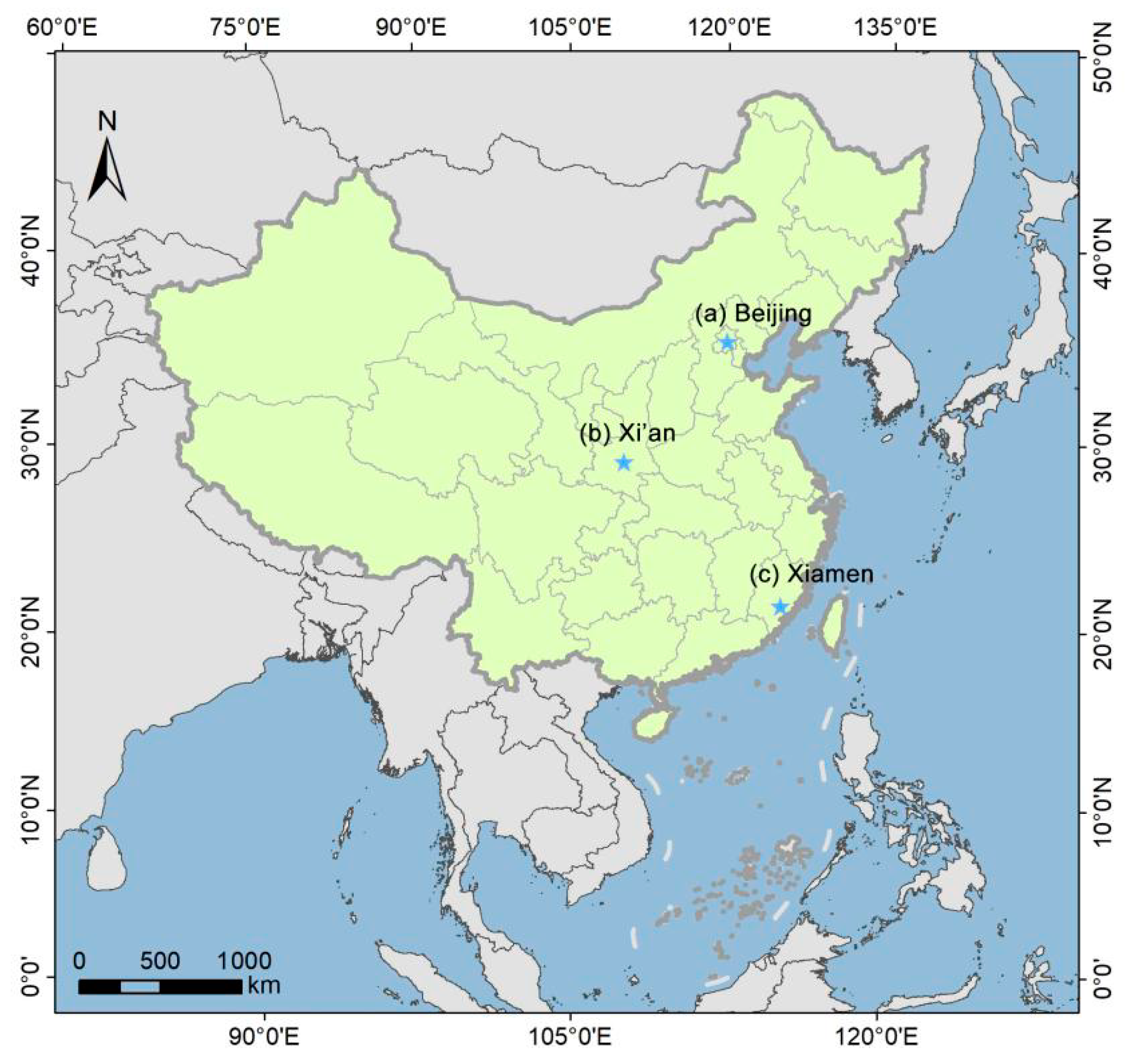
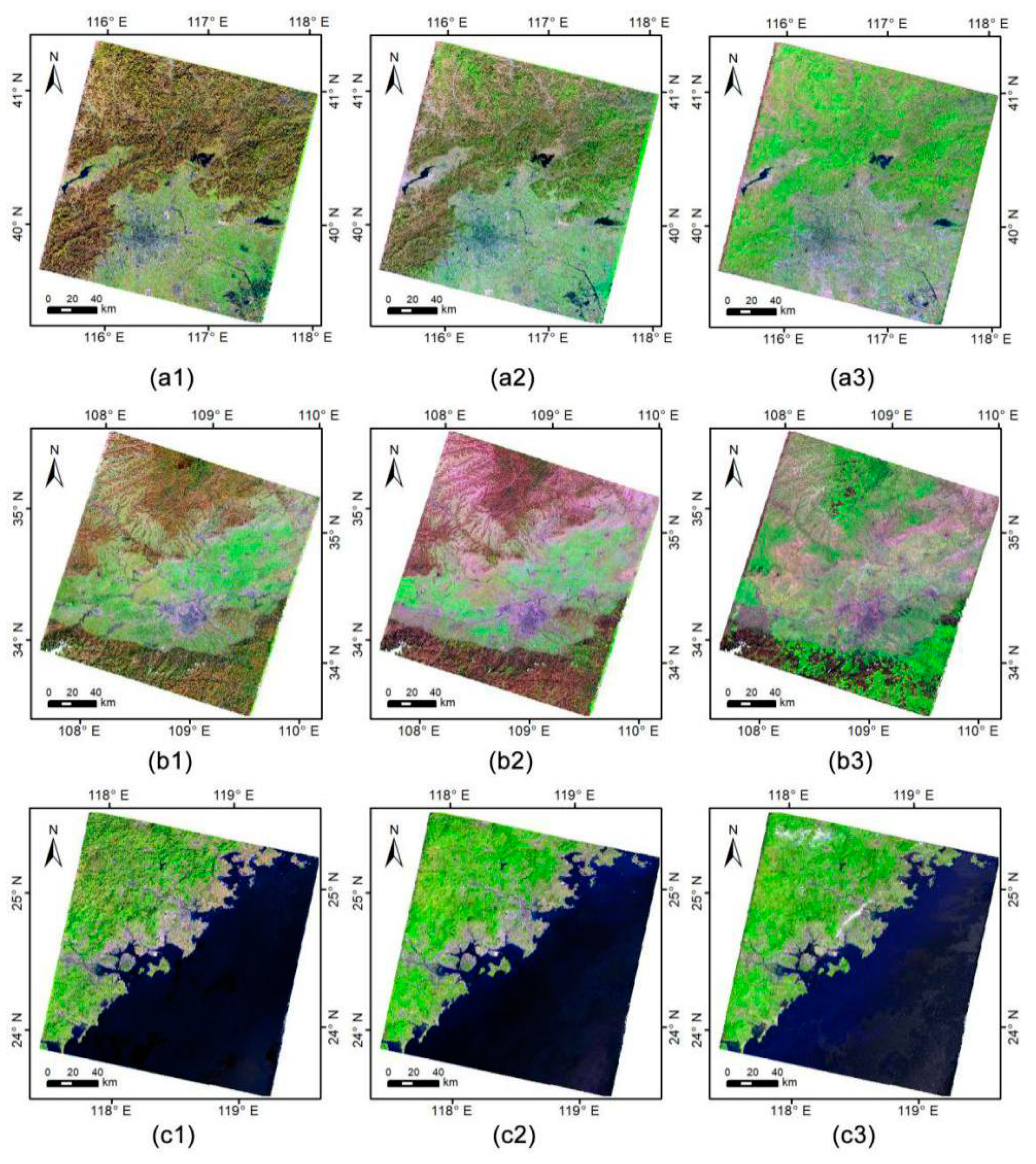
2. Dataset and Study Area
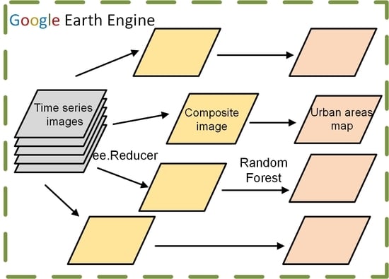
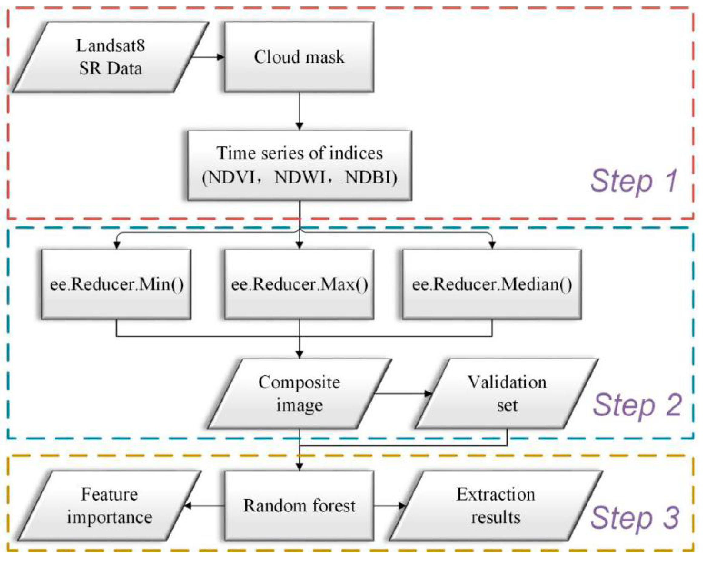
China has seen rapid urbanization and the largest human migration in history [25], particularly in the early 21st century. Three cities in China were selected as the study area, namely Beijing, Xi’an, and Xiamen (Figure 1). Beijing is the capital of China and the central city in North China, with a typical warm temperate semihumid continental monsoon climate [26]. It is hot and rainy in summer and cold and dry in winter. It is one of the ancient capitals of China with a history of more than 3000 years. Xi’an is a central city in northwestern China, with a warm and semihumid continental monsoon climate. Its history is very long, and it is also a “World Historic City” determined by the United Nations Educational, Scientific and Cultural Organization (UNESCO) in 1981. Xiamen is a central city in East China, with a subtropical maritime monsoon climate. It is a coastal city that has been rapidly developing in recent decades. For each city, a track number (path/row) was selected as the mapping area based on Landsat World Reference System II (WRS II) frames. The Landsat 8 OLI surface reflectance images corresponding to the three study areas were collected by GEE, and detailed statistics of these images are indicated in Table 1. The selected dataset is LC08/C01/T1_SR, which is the atmospherically corrected surface reflectance from the Landsat 8 OLI sensor. The images we used contained 5 visible and near-infrared bands (Coastal, Blue, Green, Red, and NIR) and 2 short-wave infrared bands (SWIR1 and SWIR2) processed to orthorectified surface reflectance.

3. Methods

The flowchart of this research is shown in Figure 2, which includes three steps. In the first step, the Quality Assessment (QA) band of the LC08/C01/T1_SR dataset, which was generated by the CFMask algorithm [27], was used for masking clouds and cloud shadows. Three indices, including the normalized difference water index (NDWI) [28], normalized difference vegetation index (NDVI) [29], and normalized difference built-up index (NDBI) [30], were calculated from the annual time series Landsat images after cloud masking. Then, in the second step, an annual composite image was obtained by the multidimensional arrays [22] for analyzing geoscience data using GEE. Three reducer functions, ee.Reducer.min(), ee.Reducer.median(), and ee.Reducer.max() provided by GEE, were selected to construct four schemes to synthesize the annual intensive time series Landsat data for each study area. Each study area can get four annual composite images. Finally, the random forest algorithm was employed as a supervised classification and feature importance evaluation method for the four annual composite images in each study area. The performances of different annual composite images in mapping urban areas were comprehensively compared and analyzed for each study area. The 68 images required for the research did not need to be downloaded locally.

3.1. Indices for Urban Areas Mapping

NDWI, NDVI, and NDBI were employed in this study. Calculations of these indices are as follows:
N D W I = G r e e n N I R / G r e e n + N I R
N D V I = N I R R e d / N I R + R e d
N D B I = S W I R N I R / S W I R + N I R
where Green, Red, NIR, and SWIR represent land surface reflectance in green, red, near-infrared, and short-wave infrared bands, respectively.

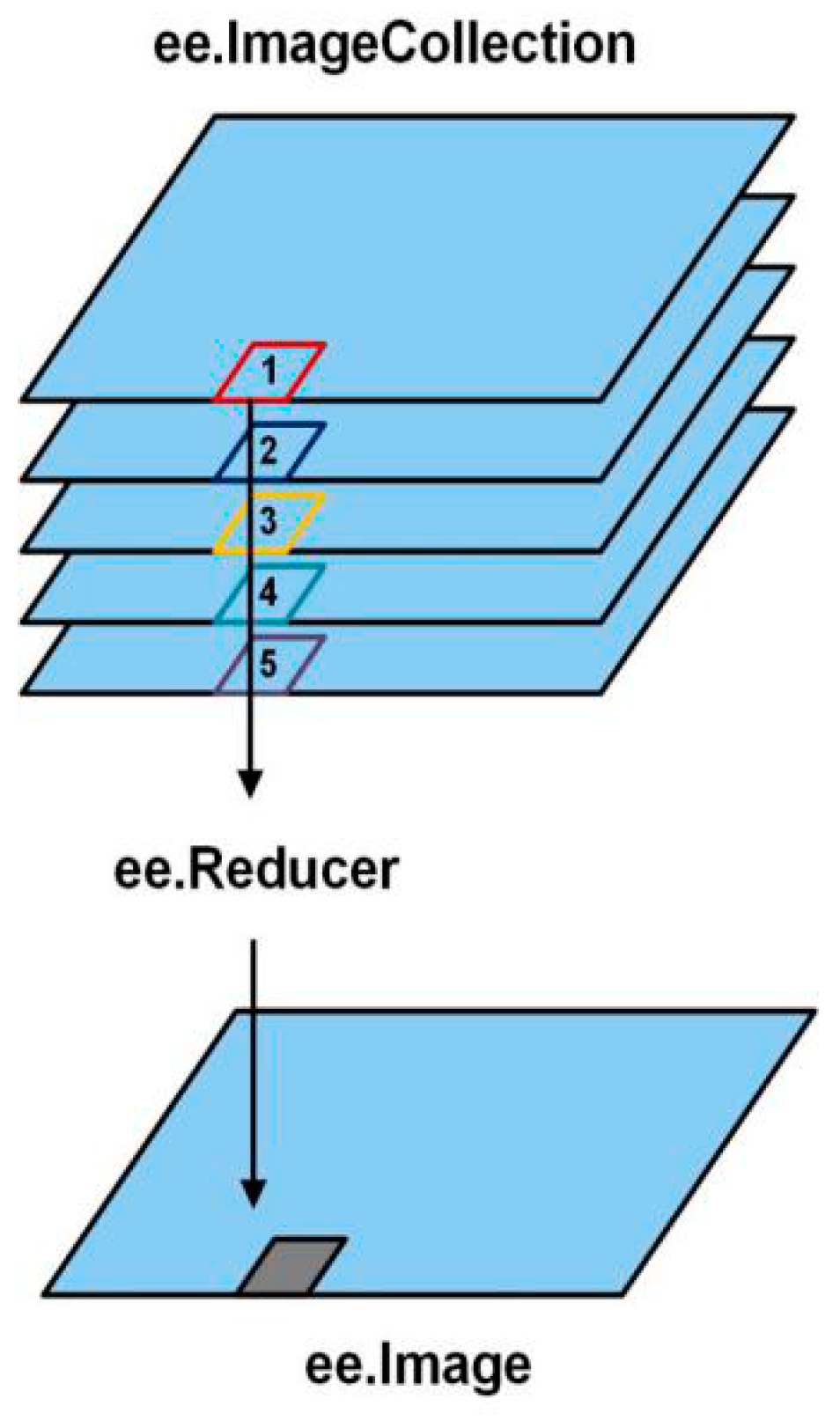
3.2. Annual Composite Image

Time series data in remote sensing have columns and rows, establishing arrays of two or more dimensions. The size and variety of Earth observation data continue to increase, which requires big data management tools and analysis methods. High-dimensional data usually contain duplicate information, which is mixed with signals and is burdensome for calculation and data storage. In order to stimulate analytics of Earth observation datasets in the big data era (e.g., time series images of Landsat 8 OLI), Lu at al. [22] put forward an array-based modeling theory, namely, multidimensional arrays, which is used to analyze geoscientific data. The emphasis in this study was the reducer operation. The reducer operations yield a meaningful array for high-dimensional data by particular aggregation functions, for example, simple statistics such as calculating the median of the data. The reducer operation plays an important role in dimension reduction and makes the data comprehensible and presentable [15]. It also benefits in terms of decreasing the required computation time and computational resources. Application of reducer operating by GEE yielded annual composite images from time series images of Landsat 8 OLI in this study.
Devised for multidimensional data, the ee.Reducer function in GEE is an often-used class that uses multidimensional arrays to combine time series data. Figure 3 explains the function of ee.Reducer, and Table 2 presents some ee.Reducer functions provided by GEE. The three reducer functions provided by GEE were selected to construct four schemes (see Table 3) to compose the annual intensive time series Landsat 8 OLI data for the three cities. In Table 3, schemes of (1)–(3) only used one reducer function to composite the spectral bands (SWIR1, SWIR2, Coastal, Blue, Green, Red, and NIR) of annual time series data to obtain an image with seven bands; however, schemes of (4) used the combination of three reducer functions to compose the NDVI, NDWI, and NDBI of time series data to obtain an image with nine bands for each study area. For example, for NDVI, a combination of reducer functions was used to extract the maximum, minimum, and median values of NDVI annual time series data.

3.3. Classification and Accuracy Assessment

Supervised classification methods [31] can evidently enhance the efficiency of urban areas mapping. Based on the evaluation of the stability performance and feature importance, the RF algorithm [32] was chosen for supervised classification at the pixel level in this research. The RF method includes a large number of parameters. The number of variables to be selected for the best split when growing the trees (Mtry) and the number of decision trees to be generated (Ntree) are two important parameters to produce the forest trees [23]. More details regarding the parameters and properties of the default values can be found in Tyralis et al.’s work [33]. In this research, an open-source platform named scikit-learn [34] was employed to implement the RF with Python. The Ntree parameter was assigned to 500, and Mtry was assigned to the square root of the number of input variables, as is usual. Other parameters were assigned to default values. Variable importance estimation is also one of the important advantages of random forest algorithms and is widely used in feature selection. After classification, we conducted a variable importance estimation.
Accuracy assessment based on the error matrix is the most typically used method [35]. Statistically robust and transparent approaches play an important role in ensuring the reliability of accuracy assessment [36]. One hundred random verification points were generated for each type using stratified random sampling, and the total validation points for urban and nonurban areas were 300 for each study area. Then, these points were verified based on annual time series Landsat 8 data and high-resolution Google Earth images for each classification result. Derived from the error matrices, the four typically used accuracy measure indices [36,37] are overall accuracy (OA), commission error ratio (CE), omission error ratio (OE), and kappa coefficients (K).

4. Results and Discussion

The performance results of the annual composites from GEE for each study area were firstly assessed through visual comparisons. Subsequently, detailed comparisons of the statistical characteristics of the samples from different composite results were performed to characterize the features of urban areas and other objects. Finally, the performance of the urban areas extraction for each study area was verified through visual comparisons and four accuracy measures from error matrices.

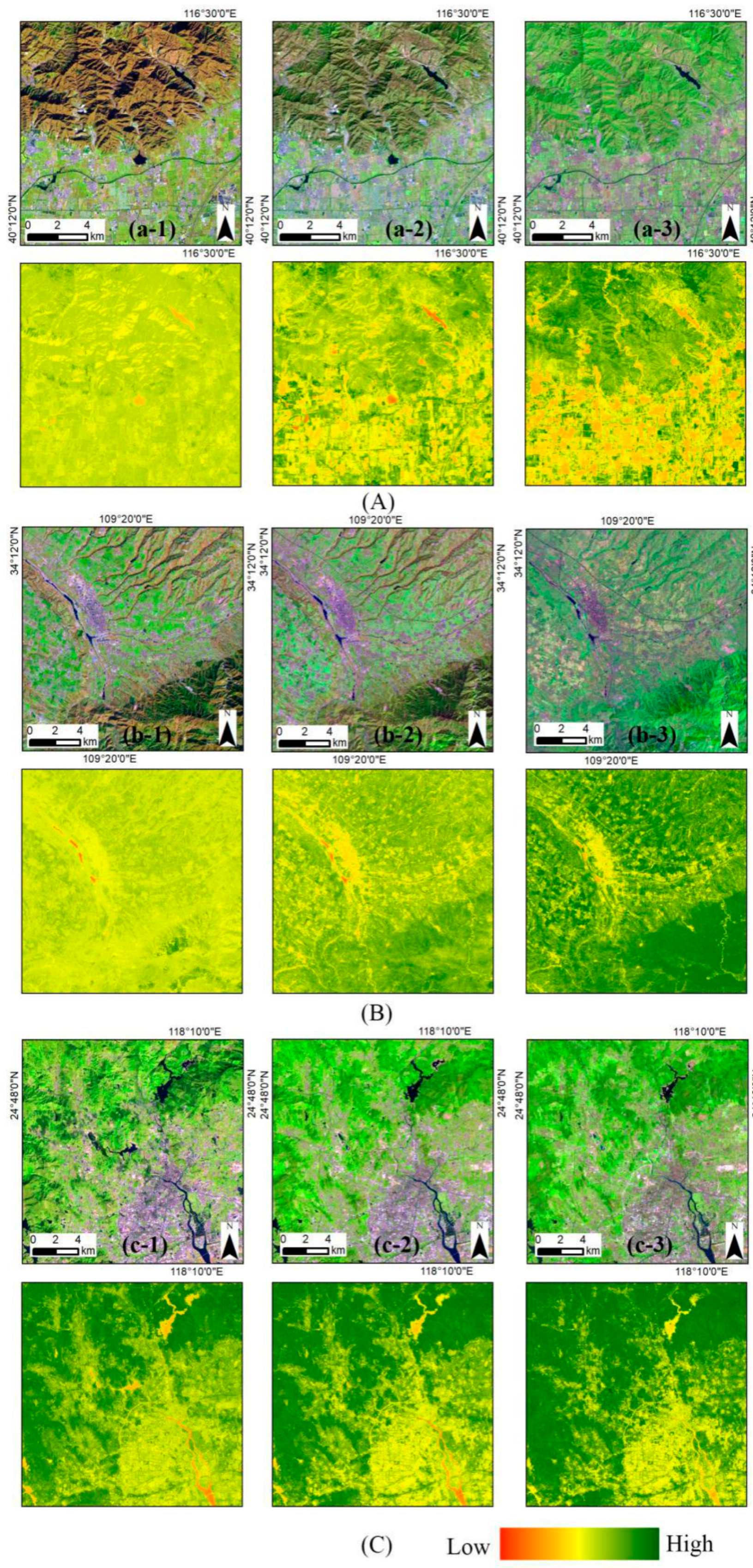
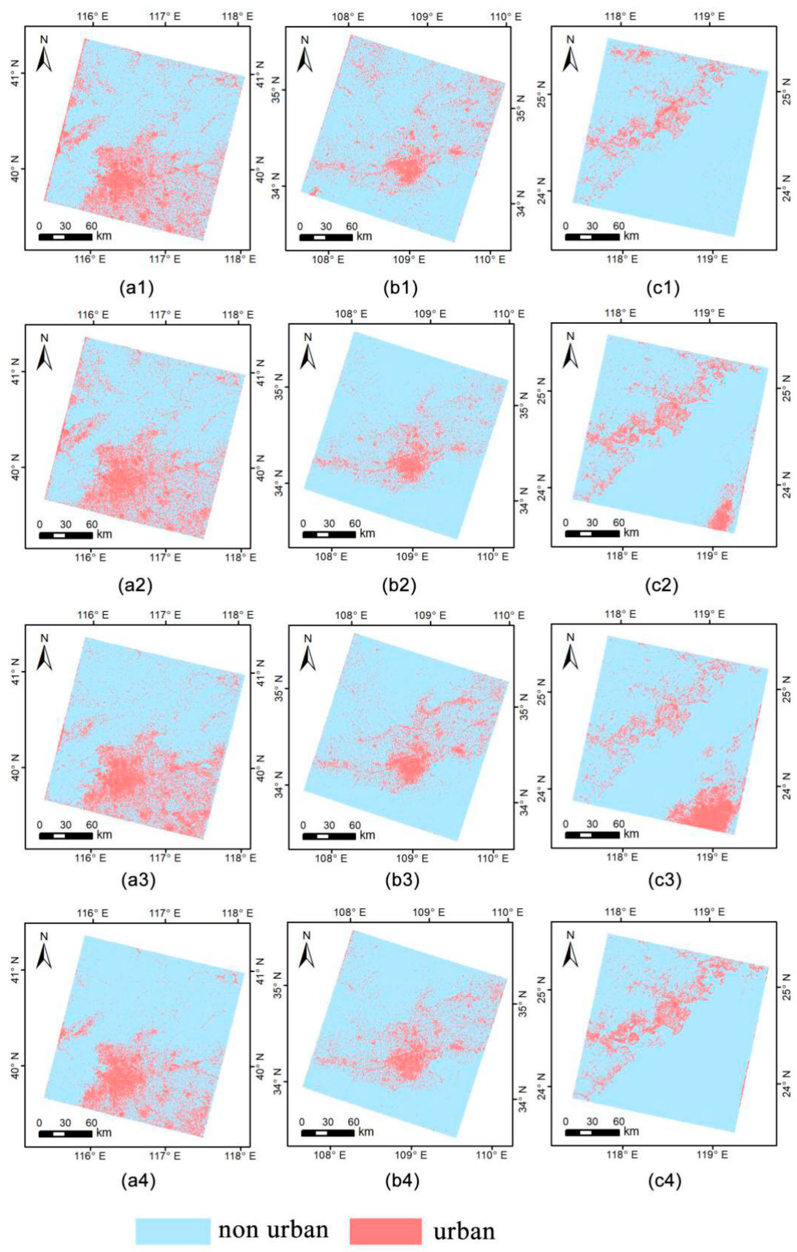
4.1. Annual Composite Result

The annual composite images of the three study areas are displayed in Figure 4. It can be clearly seen that most of the composite images have mitigated data quality influencing factors, such as residual clouds and cloud shadows. Thus, the performance of urban mapping may be improved, especially in cloudy areas. Meanwhile, the three composite images calculated by selected reducer functions, namely ee.Reducer.min(), ee.Reducer.median(), and ee.Reducer.max(), can reflect the phenological effect at each study area; however, this cannot be achieved by the single-temporal image. More specifically, the three composite images of Beijing and Xi’an exhibit more differences than Xiamen due to their greater climatic and vegetation variations in different seasons.
NDVI is an important vegetation index, reflecting plant growth and other information [38]. The NDVI images in the three study areas using the three reducers (e.g., ee.Reducer.min(), ee.Reducer.median(), and ee.Reducer.max(), respectively) are displayed in Figure 5. Based on visual inspection, the NDVI images changed obviously in Beijing and Xi’an in 2017 due to their typical warm temperate semihumid continental monsoon climate. However, NDVI images in Xiamen exhibited much fewer differences because Xiamen belongs to the subtropical marine monsoon climate, and vegetation is evergreen in different seasons.

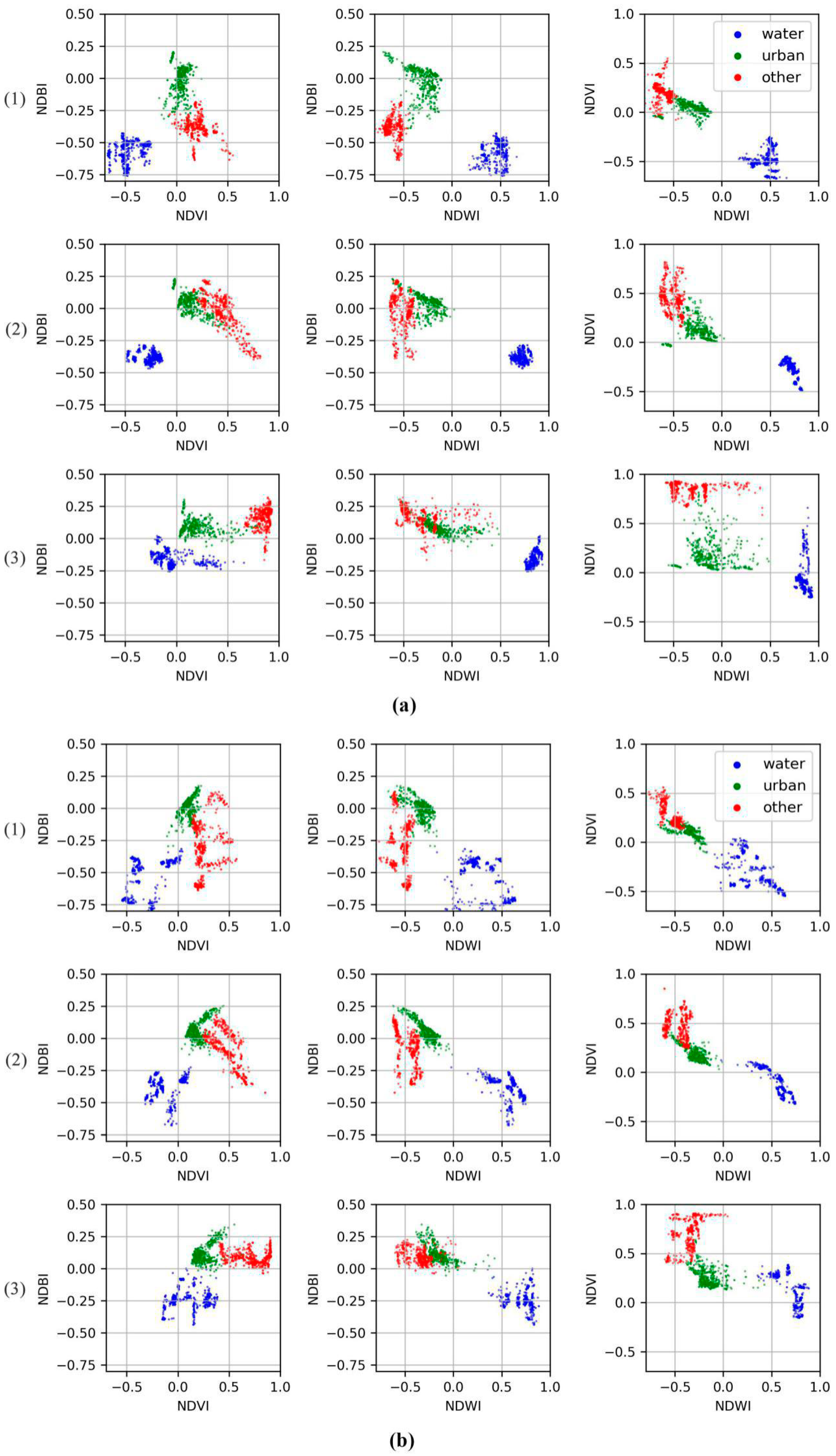
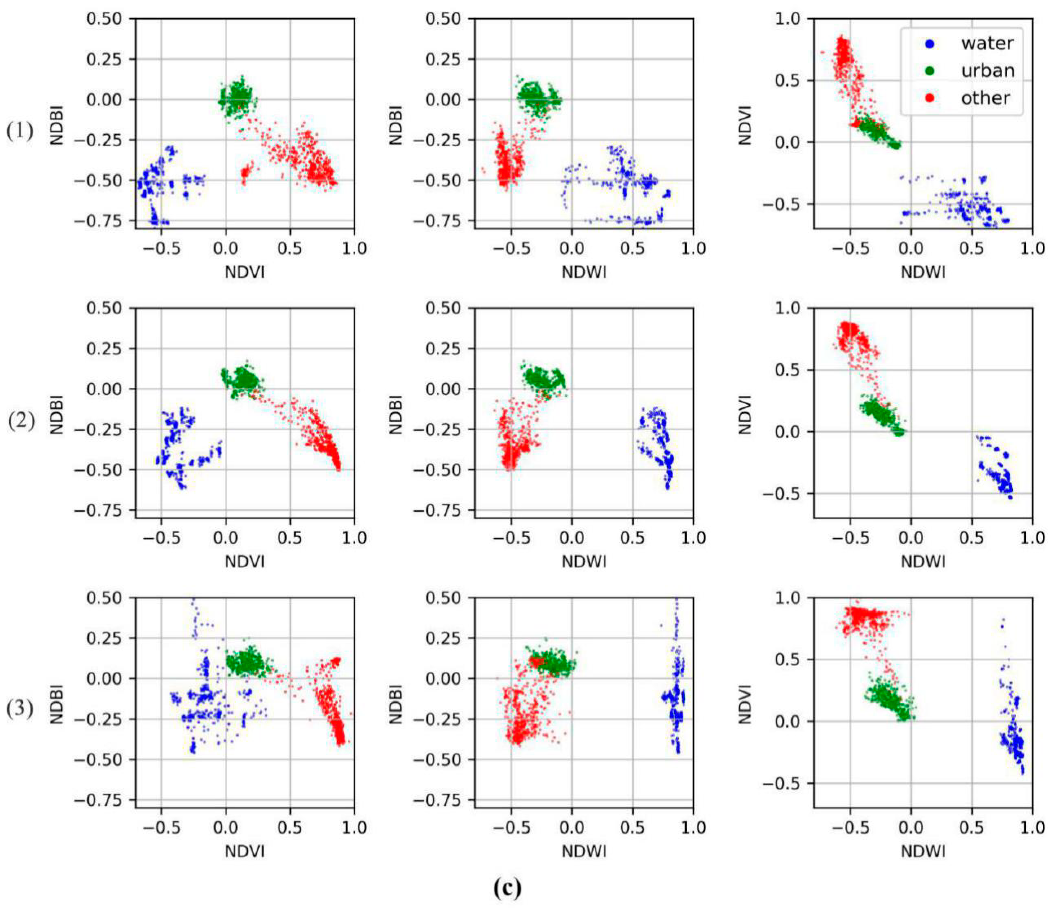
4.2. Sample Analysis

In the three study areas, the major land cover types include farmland, grassland, forest, water, bare land, and urban areas. Specifically, we referred to the definition of urban from Schneider [39]: a place dominated by the built environment, containing artificial cover and structures, such as roads and buildings. “Dominated” means that the coverage of the built environment in each pixel exceeds 50%. Combining the performance of the classifier with the time series spectral characteristics of the features, the ground objects were divided into three types: water, urban, and other (forest, grassland, farmland, etc.). Based on the above knowledge, sample points for training were selected. Through visual interpretation of annual time series Landsat 8 data and high-resolution satellite images in Google Earth, stable training samples were collected. “Stable” indicates that the type of the sampling point did not change in 2017. For each type, 500 training sample points were selected manually in each study area. The spatial distribution of these points is relatively uniform.
The scatter plots of the training sample points are the most simple and straightforward charts for assessing the separability and correlation of various training samples [40]. Figure 6 shows the training sample points of urban land along with two other types of nonurban sample points collected from images of Beijng, Xi’an, and Xiamen. It is evident that the urban samples group has unique characteristics with relatively larger NDBI values, negative NDWI values, and NDVI values close to 0. Furthermore, nonurban sample points, especially for the other type (containing farmland, forests, grasslands, etc.), change obviously in terms of NDVI, NDWI, and NDBI values by Analysis of Variance (ANOVA), which is quite different from the urban samples (see Figure 6). This is because the other types (containing farmland, forests, grasslands, etc.) change dynamically with the seasons, but urban areas have no seasonal effects.

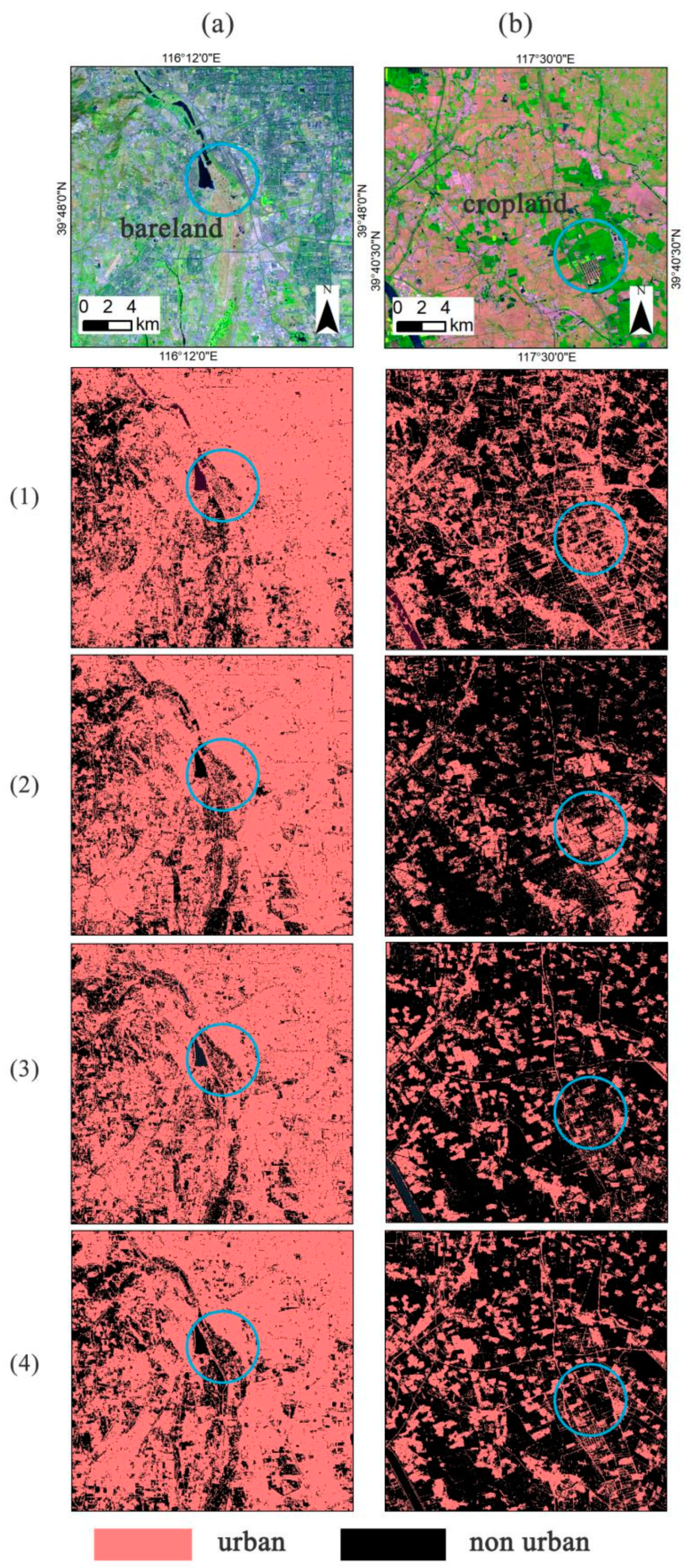
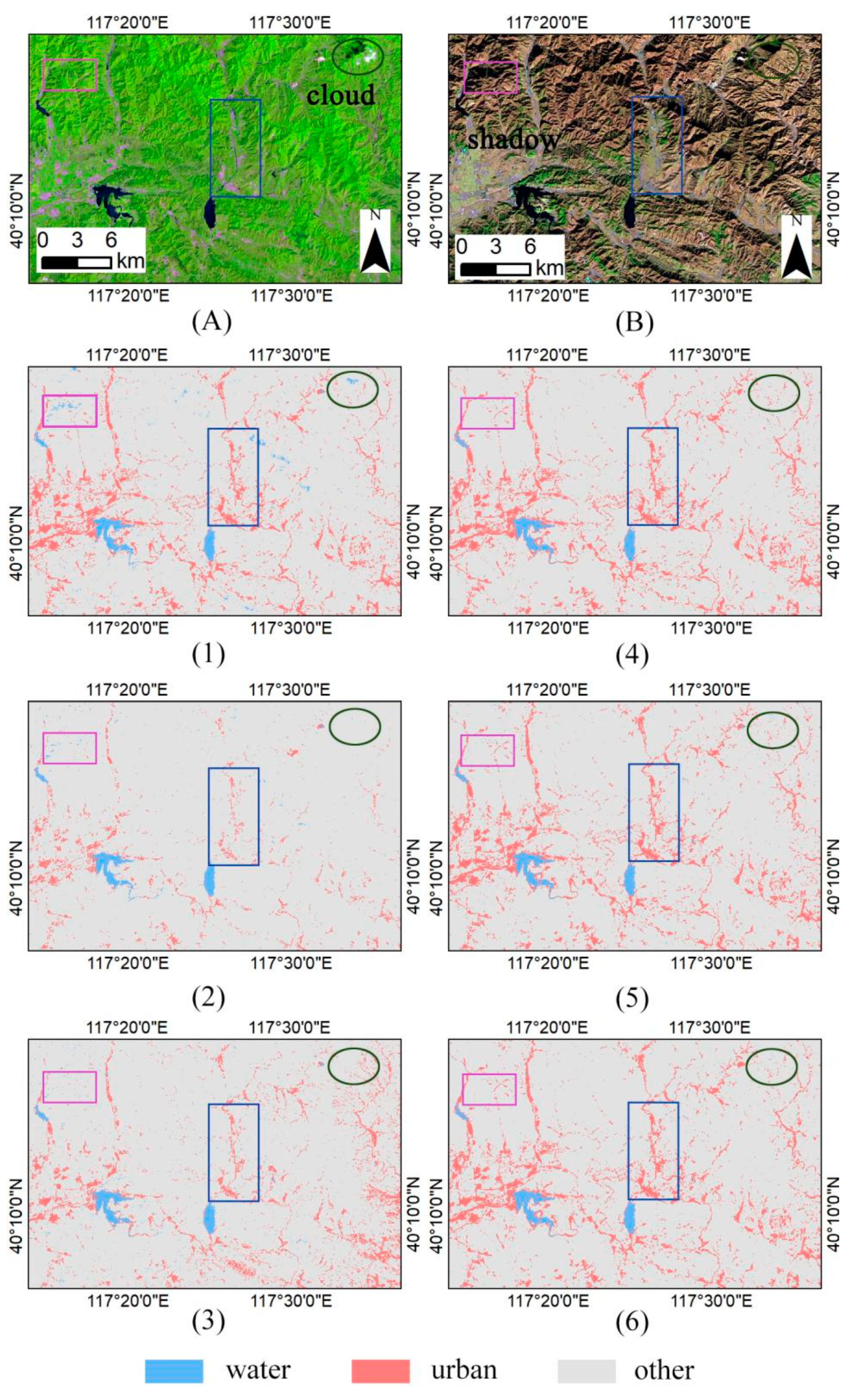
4.3. Classification Results and Accuracy Verification

Before detailed verification is undertaken, a basic visual inspection should be conducted to identify obvious errors in the classification results [41]. The classifications of the urban areas using the four schemes in the three study areas are displayed in Figure 7. Based on visual inspection, the performances in study areas a and b using the four schemes were different but did not have a significant error. The performance in study area c using the second and third schemes was unsatisfactory, with obvious errors (large urban areas on the sea) (see Figure 7(c2),(c3)).
The error matrix for the urban classification for each scene was constructed with the validation points and classification results. The assessment results are shown in Table 4. When comparing the OA, CE, OE, and K of the four schemes in the three research areas, the accuracy of the fourth scheme was better than the other schemes. Thus, the fourth scheme (the combination of multiple reducer functions) is more appropriate for urban areas extraction due to its consideration of phenological characteristics.

4.4. Performance Comparison when Suppressing Noise

Bare lands and croplands are the main sources of noise [42] in urban areas mapping from remote sensing images due to their similarities with urban areas in the spectrum. To examine the reliability of the four schemes in urban areas extraction, two major noisy images, including bare lands and croplands, were derived from the study datasets. Performance comparisons of the results of the four schemes are shown in Figure 8. For bare lands, the results in Figure 8(a3),(a4) demonstrate that bare lands can be removed using the third and fourth schemes, and the fourth scheme had the best performance. For croplands, the results in Figure 8(b1),(b2) show that croplands cannot be removed using the first and second schemes; however, the fourth scheme achieved a satisfactory result. In short, the fourth scheme performed generally well in suppressing noises.

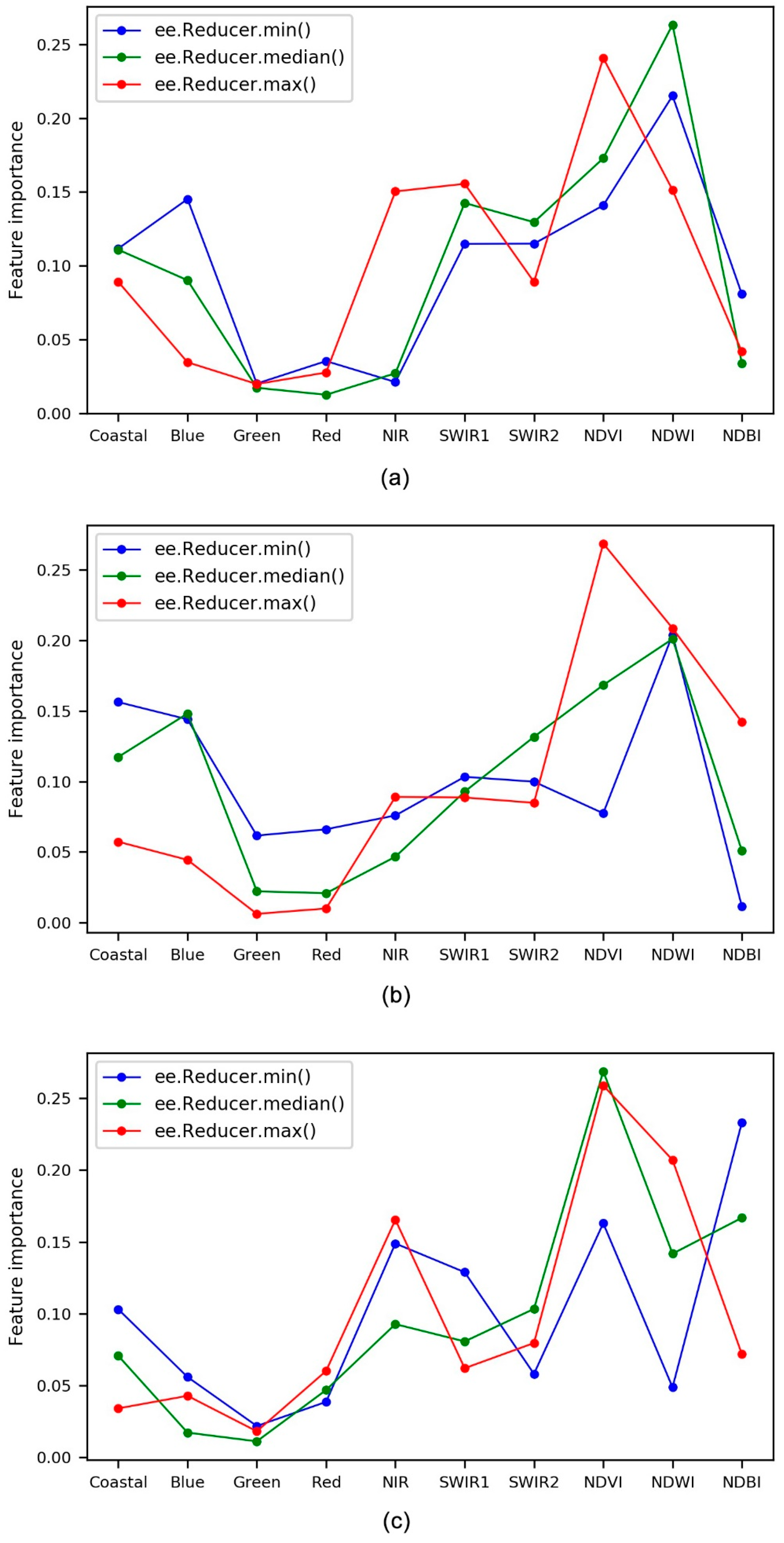
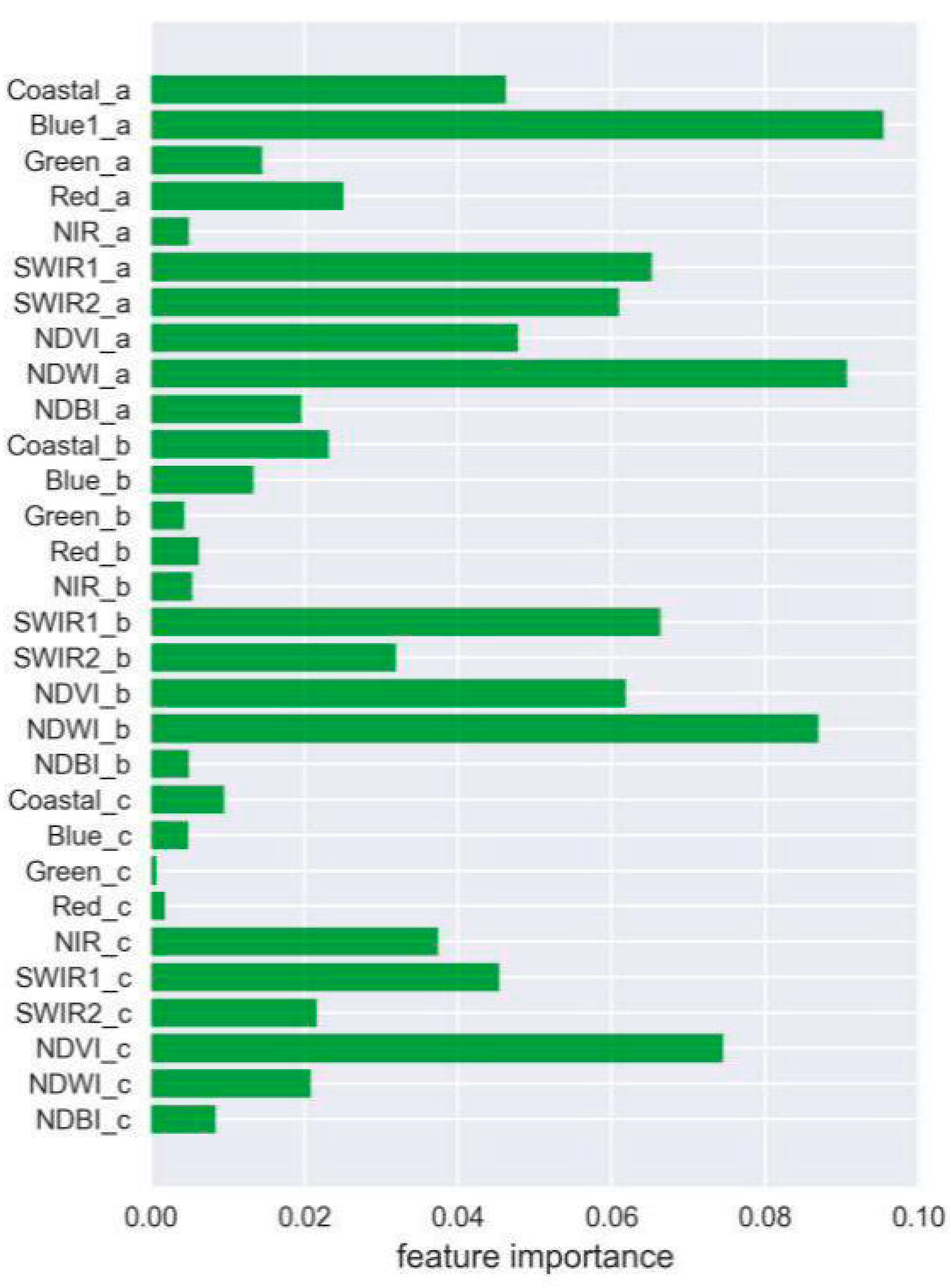
4.5. Feature Importance Evaluation

After training by random forest, the normalized feature importance of each variable can be outputted; that is, the sum of all feature importance is 1 [24]. The feature importance can be calculated internally in multiple ways, such as using the mean decrease in the Gini coefficient [32]. The greater the feature importance, the more important the feature is, and vice versa. Figure 9 shows the feature importance of the results derived from the ee.Reducer.min(), ee.Reducer.median(), and ee.Reducer.max() functions for each study area. It can be seen that although the three study areas are in different places and have different climatic conditions, they had similar characteristics in feature importance. NDVI and NDWI were the most important features, followed by Coastal, Blue, NIR, SWIR1, and SWIR2 bands, and the Green and Red bands exhibited relatively less importance. Figure 10 shows the feature importance with all 30 predictor variables in Beijing. It can also be found that SWIR1, SWIR2, NDVI, and NDWI were more important features.

4.6. Performance of Multiple Reducer Functions

Urban areas mapping simply based on a single reducer function contains great uncertainties because of spectral confusions among different land cover types, and these limitations may be mitigated by applying multiple reducer functions to synthesize images. To further examine the performance of the synthetic images based on multiple reducer functions, the other two synthesis schemes were selected for urban areas mapping in Beijing (see Table 5). Scheme (5) used images in two different seasons (summer and winter) for urban areas mapping, and scheme (6) selected relatively important features. The assessment results are also summarized in Table 5. Schemes (4)–(6) employed multiple reducer functions, but the others employed only one. As can be seen from Table 4, Table 5, when comparing the OA, K, OE, and CE of the six schemes in Beijing, the accuracy of the schemes using multiple reducer functions was higher. Performance comparisons of the six schemes are shown in Figure 11. It can be found that the schemes using multiple reducer functions had fewer omission situations for urban mapping and better performance in suppressing cloud and mountain shadows. In short, the schemes using multiple reducer functions generally performed better in urban areas mapping.

5. Conclusions

Big data streams in remote sensing are reforming urban areas mapping. In particular, long-term sequence-based satellite observations provide sufficient data for urban remote sensing by GEE. This study employed composite images extracted by four schemes to extract urban areas at GEE. Three study areas in China were selected, and random forest was applied as a supervised classification at the pixel level to map urban areas. The performances of urban areas extraction and noise suppression were comprehensively compared for each study area. In this research, we attempted to determine how effectively annual time series images from Landsat 8 OLI can be composed for urban areas mapping in only three cities in China, and the work can be used as a reference for other cities and even other land cover mapping studies. Some conclusions can be made from this research as follows:
First, temporal information is crucial for urban areas mapping. Urban areas mapping simply based on a single reducer function contains great uncertainties because of spectral confusion among different land cover types, and these limitations can be obviously mitigated by applying a combination of multiple reducer functions to synthesize images.
Second, vegetation and water indices, including NDVI and NDWI, are significant features to identify urban areas based on the feature importance evaluation of the random forest (see Figure 9, Figure 10).
While most urban areas maps are based on daytime optical and thermal sensors such as Landsat 8 OLI/TIRS, there are other sensors that also supply distinctive observations for urban areas, including but not limited to nighttime light sensors, LiDAR, and RADAR. GEE provides high-performance parallel computing capabilities to process annual dense time series data while storing multiple petabyte (PB)-level datasets including remote sensing and other data. If combined with multisource remote sensing data and multiple reducer functions by GEE, the accuracy of urban areas mapping can be further improved.

Author Contributions

Z.Z. and D.P. conceived and designed the experiments. D.P., M.W., G.W. and T.L. performed the experiments and analyzed the data. Z.Z., D.P., G.H. and M.W. wrote the whole paper, and all authors edited the paper. All authors have read and agreed to the published version of the manuscript.

Funding

This research was funded by the National Natural Science Foundation of China, grant number 61731022; the Strategic Priority Research Program of the Chinese Academy of Sciences, grant number XDA19090300; and the National Key Research and Development Program of China, grant numbers 2016YFA0600302 and 2016YFB0501502.

Data Availability Statement

Not applicable.

Conflicts of Interest

The authors declare no conflict of interest.

References

  1. Grimm, N.B.; Faeth, S.H.; Golubiewski, N.E.; Redman, C.L.; Wu, J.; Bai, X.; Briggs, J.M. Global change and the ecology of cities. Science 2008, 319, 756–760. [Google Scholar] [CrossRef] [PubMed] [Green Version]
  2. Rodriguez, R.S. Sustainable Development Goals and climate change adaptation in cities. Nat. Clim. Chang. 2018. [Google Scholar] [CrossRef]
  3. Weng, Q. Remote sensing of impervious surfaces in the urban areas: Requirements, methods, and trends. Remote Sens. Environ. 2012, 117, 34–49. [Google Scholar] [CrossRef]
  4. Qihao, W.; Xuefei, H. Medium Spatial Resolution Satellite Imagery for Estimating and Mapping Urban Impervious Surfaces Using LSMA and ANN. IEEE Trans. Geosci. Remote Sens. 2008, 46, 2397–2406. [Google Scholar] [CrossRef]
  5. Seto, K.C.; Fragkias, M. Quantifying Spatiotemporal Patterns of Urban Land-use Change in Four Cities of China with Time Series Landscape Metrics. Landsc. Ecol. 2005, 20, 871–888. [Google Scholar] [CrossRef]
  6. Lu, D.; Tian, H.; Zhou, G.; Ge, H. Regional mapping of human settlements in Southeastern China with multisensor remotely sensed data. Remote Sens. Environ. 2008, 112, 3668–3679. [Google Scholar] [CrossRef]
  7. Im, J.; Lu, Z.; Rhee, J.; Quackenbush, L.J. Impervious surface quantification using a synthesis of artificial immune networks and decision/regression trees from multi-sensor data. Remote Sens. Environ. 2012, 117, 102–113. [Google Scholar] [CrossRef]
  8. Ban, Y.; Jacob, A.; Gamba, P. Spaceborne SAR data for global urban mapping at 30m resolution using a robust urban extractor. ISPRS J. Photogramm. Remote Sens. 2015, 103, 28–37. [Google Scholar] [CrossRef]
  9. Zhu, Z.; Woodcock, C.E.; Rogan, J.; Kellndorfer, J. Assessment of spectral, polarimetric, temporal, and spatial dimensions for urban and peri-urban land cover classification using Landsat and SAR data. Remote Sens. Environ. 2012, 117, 72–82. [Google Scholar] [CrossRef]
  10. Schneider, A.; Friedl, M.A.; Potere, D. Mapping global urban areas using MODIS 500-m data: New methods and datasets based on ‘urban ecoregions’. Remote Sens. Environ. 2010, 114, 1733–1746. [Google Scholar] [CrossRef]
  11. Zhao, Y.; Feng, D.; Yu, L.; Wang, X.; Chen, Y.; Bai, Y.; Hernández, H.J.; Galleguillos, M.; Estades, C.; Biging, G.S.; et al. Detailed dynamic land cover mapping of Chile: Accuracy improvement by integrating multi-temporal data. Remote Sens. Environ. 2016, 183, 170–185. [Google Scholar] [CrossRef]
  12. Khatami, R.; Mountrakis, G.; Stehman, S.V. A meta-analysis of remote sensing research on supervised pixel-based land-cover image classification processes: General guidelines for practitioners and future research. Remote Sens. Environ. 2016, 177, 89–100. [Google Scholar] [CrossRef] [Green Version]
  13. Maxwell, S.K.; Sylvester, K.M. Identification of “ever-cropped” land (1984–2010) using Landsat annual maximum NDVI image composites: Southwestern Kansas case study. Remote Sens. Environ. 2012, 121, 186–195. [Google Scholar] [CrossRef] [Green Version]
  14. Li, X.; Gong, P.; Liang, L. A 30-year (1984–2013) record of annual urban dynamics of Beijing City derived from Landsat data. Remote Sens. Environ. 2015, 166, 78–90. [Google Scholar] [CrossRef]
  15. Appel, M.; Lahn, F.; Buytaert, W.; Pebesma, E. Open and scalable analytics of large Earth observation datasets: From scenes to multidimensional arrays using SciDB and GDAL. ISPRS J. Photogramm. Remote Sens. 2018, 138, 47–56. [Google Scholar] [CrossRef]
  16. Kumar, L.; Mutanga, O. Google Earth Engine Applications Since Inception: Usage, Trends, and Potential. Remote Sens. 2018, 10, 1509. [Google Scholar] [CrossRef] [Green Version]
  17. Gorelick, N.; Hancher, M.; Dixon, M.; Ilyushchenko, S.; Thau, D.; Moore, R. Google Earth Engine: Planetary-scale geospatial analysis for everyone. Remote Sens. Environ. 2017, 202, 18–27. [Google Scholar] [CrossRef]
  18. Xiong, J.; Thenkabail, P.S.; Gumma, M.K.; Teluguntla, P.; Poehnelt, J.; Congalton, R.G.; Yadav, K.; Thau, D. Automated cropland mapping of continental Africa using Google Earth Engine cloud computing. ISPRS J. Photogramm. Remote Sens. 2017, 126, 225–244. [Google Scholar] [CrossRef] [Green Version]
  19. Long, T.; Zhang, Z.; He, G.; Jiao, W.; Tang, C.; Wu, B.; Zhang, X.; Wang, G.; Yin, R. 30 m Resolution Global Annual Burned Area Mapping Based on Landsat Images and Google Earth Engine. Remote Sens. 2019, 11, 489. [Google Scholar] [CrossRef] [Green Version]
  20. Huang, M.; Chen, N.; Du, W.; Chen, Z.; Gong, J. DMBLC: An Indirect Urban Impervious Surface Area Extraction Approach by Detecting and Masking Background Land Cover on Google Earth Image. Remote Sens. 2018, 10, 766. [Google Scholar] [CrossRef] [Green Version]
  21. Huang, H.; Chen, Y.; Clinton, N.; Wang, J.; Wang, X.; Liu, C.; Gong, P.; Yang, J.; Bai, Y.; Zheng, Y.; et al. Mapping major land cover dynamics in Beijing using all Landsat images in Google Earth Engine. Remote Sens. Environ. 2017, 202, 166–176. [Google Scholar] [CrossRef]
  22. Lu, M.; Appel, M.; Pebesma, E. Multidimensional Arrays for Analysing Geoscientific Data. ISPRS Int. J. Geo Inf. 2018, 7, 313. [Google Scholar] [CrossRef] [Green Version]
  23. Rodriguez-Galiano, V.F.; Chica-Olmo, M.; Abarca-Hernandez, F.; Atkinson, P.M.; Jeganathan, C. Random Forest classification of Mediterranean land cover using multi-seasonal imagery and multi-seasonal texture. Remote Sens. Environ. 2012, 121, 93–107. [Google Scholar] [CrossRef]
  24. Belgiu, M.; Drăguţ, L. Random forest in remote sensing: A review of applications and future directions. ISPRS J. Photogramm. Remote Sens. 2016, 114, 24–31. [Google Scholar] [CrossRef]
  25. Gong, P.; Liang, S.; Carlton, E.J.; Jiang, Q.; Wu, J.; Wang, L.; Remais, J.V. Urbanisation and health in China. Lancet 2012, 379, 843–852. [Google Scholar] [CrossRef]
  26. Wang, S.; Zhang, X.; Wu, T.; Yang, Y. The evolution of landscape ecological security in Beijing under the influence of different policies in recent decades. Sci. Total Environ. 2019, 646, 49–57. [Google Scholar] [CrossRef] [PubMed]
  27. Foga, S.; Scaramuzza, P.L.; Guo, S.; Zhu, Z.; Dilley, R.D.; Beckmann, T.; Schmidt, G.L.; Dwyer, J.L.; Joseph Hughes, M.; Laue, B. Cloud detection algorithm comparison and validation for operational Landsat data products. Remote Sens. Environ. 2017, 194, 379–390. [Google Scholar] [CrossRef] [Green Version]
  28. McFeeters, S.K. The use of the Normalized Difference Water Index (NDWI) in the delineation of open water features. Int. J. Remote Sens. 1996, 17, 1425–1432. [Google Scholar] [CrossRef]
  29. Chen, J.M.; Cihlar, J. Retrieving leaf area index of boreal conifer forests using Landsat TM images. Remote Sens. Environ. 1996, 55, 153–162. [Google Scholar] [CrossRef]
  30. Zha, Y.; Gao, J.; Ni, S. Use of normalized difference built-up index in automatically mapping urban areas from TM imagery. Int. J. Remote Sens. 2003, 24, 583–594. [Google Scholar] [CrossRef]
  31. Heydari, S.S.; Mountrakis, G. Effect of classifier selection, reference sample size, reference class distribution and scene heterogeneity in per-pixel classification accuracy using 26 Landsat sites. Remote Sens. Environ. 2018, 204, 648–658. [Google Scholar] [CrossRef]
  32. Breiman, L. Random Forests. In Machine Learning; Springer: Berlin/Heidelberg, Germany, 2001. [Google Scholar]
  33. Tyralis, H.; Papacharalampous, G.; Langousis, A. A brief review of random forests for water scientists and practitioners and their recent history in water resources. Water 2019, 11, 910. [Google Scholar] [CrossRef] [Green Version]
  34. Scikit-Learn. Available online: https://scikit-learn.org/stable/index.html (accessed on 9 November 2019).
  35. Padilla, M.; Stehman, S.V.; Chuvieco, E. Validation of the 2008 MODIS-MCD45 global burned area product using stratified random sampling. Remote Sens. Environ. 2014, 144, 187–196. [Google Scholar] [CrossRef]
  36. Olofsson, P.; Foody, G.M.; Herold, M.; Stehman, S.V.; Woodcock, C.E.; Wulder, M.A. Good practices for estimating area and assessing accuracy of land change. Remote Sens. Environ. 2014, 148, 42–57. [Google Scholar] [CrossRef]
  37. Costa, H.; Foody, G.M.; Boyd, D.S. Supervised methods of image segmentation accuracy assessment in land cover mapping. Remote Sens. Environ. 2018, 205, 338–351. [Google Scholar] [CrossRef] [Green Version]
  38. Liu, B.; Chen, J.; Chen, J.; Zhang, W. Land Cover Change Detection Using Multiple Shape Parameters of Spectral and NDVI Curves. Remote Sens. 2018, 10, 1251. [Google Scholar] [CrossRef] [Green Version]
  39. Schneider, A.; Mertes, C.M. Expansion and growth in Chinese cities, 1978–2010. Environ. Res. Lett. 2014, 9, 024008. [Google Scholar] [CrossRef]
  40. Liu, X.; Hu, G.; Chen, Y.; Li, X.; Xu, X.; Li, S.; Pei, F.; Wang, S. High-resolution multi-temporal mapping of global urban land using Landsat images based on the Google Earth Engine Platform. Remote Sens. Environ. 2018, 209, 227–239. [Google Scholar] [CrossRef]
  41. Li, X.; Zhou, Y.; Zhu, Z.; Liang, L.; Yu, B.; Cao, W. Mapping annual urban dynamics (1985–2015) using time series of Landsat data. Remote Sens. Environ. 2018, 216, 674–683. [Google Scholar] [CrossRef]
  42. Li, X.; Gong, P. An “exclusion-inclusion” framework for extracting human settlements in rapidly developing regions of China from Landsat images. Remote Sens. Environ. 2016, 186, 286–296. [Google Scholar] [CrossRef]
Figure 1. The locations of the three cities in China; a, b, and c represent Beijing, Xi’an, and Xiamen, respectively.
Remotesensing 13 00748 g001
Figure 2. Overall flowchart adopted in this study.
Remotesensing 13 00748 g002
Figure 3. The reducer operation provided by Google Earth Engine (GEE) [17].
Remotesensing 13 00748 g003
Figure 4. Annual composite images of the three districts obtained in this study ((a), (b), and (c) represent Beijing, Xi’an, and Xiamen, respectively; 1, 2, and 3 represent the results from ee.Reducer.min(), ee.Reducer.median(), and ee.Reducer.max() respectively). (R: Band 6; G: Band 5; B: Band 3).
Remotesensing 13 00748 g004
Figure 5. NDVI changes in the three study areas ((A), (B), and (C) represent Beijing, Xi’an, and Xiamen, respectively; 1, 2, and 3 represent the results from ee.Reducer.min(), ee.Reducer.median(), and ee.Reducer.max(), respectively).
Remotesensing 13 00748 g005
Figure 6. The scatter plot of the training sample points for different land cover types in the feature space composed of NDWI, NDVI, and NDBI ((a), (b), and (c) represent Beijing, Xi’an, and Xiamen, respectively; (1), (2), and (3) represent the results from ee.Reducer.min(), ee.Reducer.median(), and ee.Reducer.max(), respectively).
Remotesensing 13 00748 g006aRemotesensing 13 00748 g006b
Figure 7. Urban areas mapping results comparison of the four algorithms in the three research areas ((a), (b), and (c) represent Beijing, Xi’an, and Xiamen, respectively; 1, 2, 3, and 4 represent the schemes in Table 3).
Remotesensing 13 00748 g007
Figure 8. Performance comparison in the representative cities (a,b). (The first row represents the Landsat 8 data (R: Band 6; G: Band 5; B: Band 4); 1, 2, 3, and 4 represent the schemes in Table 3).
Remotesensing 13 00748 g008
Figure 9. Feature importance by random forest in the three study areas ((a), (b), and (c) represent Beijing, Xi’an, and Xiamen, respectively).
Remotesensing 13 00748 g009
Figure 10. The feature importance with all 30 predictor variables in Beijing ((a), (b), and (c) represent the results from ee.Reducer.min(), ee.Reducer.median(), ee.Reducer.max(), respectively. Coastal, Blue, Green, Red, NIR, SWIR1, SWIR2, NDVI, NDWI, and NDBI indicate the variables used in this study).
Remotesensing 13 00748 g010
Figure 11. Performance comparisons in the representative places. ((A,B) represent the Landsat 8 data (R: Band 6; G: Band 5; B: Band 4, A is in summer, and B is in winter); (1)–(6) represent the schemes in Table 3, Table 5).
Remotesensing 13 00748 g011
Table 1. Information of the collected Landsat 8 OLI data.
Study AreaPath/RowData AcquisitionNo. of ImAgesCityMajor Noise Source
a123/32All available Landsat 8 data in 201722BeijingCroplands
b127/36All available Landsat 8 data in 201723Xi’anBare lands, Croplands
c119/43All available Landsat 8 data in 201723XiamenClouds, Cloud shadows
Table 2. Some functions of reducer operation provided by GEE [17].
ReducersExamplesMode of Operation
SimpleCount, distinct, first, etc.Context-dependent
MathematicalMin, max, sum, product, etc.
LogicalLogical, etc.
StatisticalMode, percentile, mean, median, etc.
CorrelationKendall, Spearman, etc.
RegressionLinear regression, etc.
Table 3. The four schemes for image compositing of annual time series data at each study area
SchemeReducer UseBand UseNo. of
Bands of Composite Images
(1)ee.Reducer.min()SWIR1, SWIR2, Coastal, Blue, Green, Red, NIR7
(2)ee.Reducer.median()SWIR1, SWIR2, Coastal, Blue, Green, Red, NIR7
(3)ee.Reducer.max()SWIR1, SWIR2, Coastal, Blue, Green, Red, NIR7
(4)ee.Reducer.min(),
ee.Reducer.median(),
ee.Reducer.max()
NDVI, NDBI, NDWI9
SWIR = Short-Wave Infrared Band, NIR = Near-Infrared Band, NDWI = Normalized Difference Water Index, NDVI = Normalized Difference Vegetation Index, NDBI = Normalized Difference Built-up Index.
Table 4. Accuracy evaluation of the four schemes in the three study areas ((a), (b), and (c) represent Beijing, Xi’an, and Xiamen, respectively; 1, 2, 3, and 4 represent the schemes in Table 3).
Study AreaSchemeOA (%)CE (%)OE (%)K
a(1)83.3329.2017.530.635
(2)84.0025.8918.630.652
(3)88.3321.3012.370.741
(4)94.338.187.340.878
b(1)92.3326.3216.000.739
(2)93.6717.2415.790.796
(3)91.0029.3119.610.698
(4)96.0011.868.770.872
c(1)96.3318.187.690.846
(2)91.0035.1918.600.669
(3)81.0053.1628.850.450
(4)97.3313.955.130.887
Table 5. Accuracy evaluation of the other two schemes in Beijing.
SchemeReducer UseBand UseNo. of
Bands of Composite Images
OA (%)CE (%)OE (%)K
(5)ee.Reducer.min(),
ee.Reducer.max()
Coastal, Blue, Green,
Red, NIR, SWIR1,
SWIR2, NDVI, NDWI,
NDBI
2092.3310.0010.810.835
(6)ee.Reducer.min(),
ee.Reducer.median(),
ee.Reducer.max()
SWIR1, SWIR2,
NDVI, NDWI
1295.007.346.480.892
Publisher’s Note: MDPI stays neutral with regard to jurisdictional claims in published maps and institutional affiliations.

