Spectral and Spatial Global Context Attention for Hyperspectral Image Classification

Abstract

Recently, hyperspectral image (HSI) classification has attracted increasing attention in the remote sensing field. Plenty of CNN-based methods with diverse attention mechanisms (AMs) have been proposed for HSI classification due to AMs being able to improve the quality of feature representations. However, some of the previous AMs squeeze global spatial or channel information directly by pooling operations to yield feature descriptors, which inadequately utilize global contextual information. Besides, some AMs cannot exploit the interactions among channels or positions with the aid of nonlinear transformation well. In this article, a spectral-spatial network with channel and position global context (GC) attention (SSGCA) is proposed to capture discriminative spectral and spatial features. Firstly, a spectral-spatial network is designed to extract spectral and spatial features. Secondly, two novel GC attentions are proposed to optimize the spectral and spatial features respectively for feature enhancement. The channel GC attention is used to capture channel dependencies to emphasize informative features while the position GC attention focuses on position dependencies. Both GC attentions aggregate global contextual features of positions or channels adequately, following a nonlinear transformation. Experimental results on several public HSI datasets demonstrate that the spectral-spatial network with GC attentions outperforms other related methods.

1. Introduction

Compared with traditional panchromatic and multispectral remote sensing images, hyperspectral images (HSIs) contain rich spectral information owing to the hundreds of narrow contiguous wavelength bands. In addition, some spatial information from homogeneous areas is also incorporated into HSIs. Recently, HSIs have been widely used in various kinds of fields, such as land cover mapping [1], change detection [2], object detection [3], vegetation analysis [4], etc. With the rapid development of HSI technology, HSI classification has become a hot and valuable topic, which aims at assigning each pixel vector to a specific land cover class [5,6]. Due to the curse of dimensionality and the Hughes phenomenon [7,8], how to explore the plentiful spectral and spatial information of HSIs remains extremely challenging.

To take advantage of abundant spectral information, traditional HSI classification methods tend to take an original pixel vector as the input, such as $\kappa$-nearest neighbors (KNNs) [9], multinomial logistic regression (MLR) [10], and linear discriminant analysis (LDA) [11]. These methods mainly focus on two steps: feature engineering and classifier training. Feature engineering reduces the high dimensionality of the spectral pixel vector to capture effective features. Then, the extracted features are fed into a general-purpose classifier to yield the classification results. However, these spectral-based classifiers only concern spectral information while ignoring the spatial correlation and local consistency of HSI. Later, some spectral-spatial classifiers appeared for HSI classification, such as DMP-SVM [12], Gabor-SVM [13], and SVM-MRF [14]. These methods improve the classification performance to a certain extent, such as approximately 10% overall accuracy on the popular Pavia University dataset. However, the aforementioned methods belong to shallow layer models, which have limited representation capacity to fully utilize the abundant spectral and spatial information of HSIs. Specifically, these models usually utilize handcrafted features, which cannot effectively reflect the characteristics of different objects. Consequently, they have poor adaptability to the spatial environment.

Recently, deep learning (DL) methods have achieved considerable breakthroughs in the field of computer vision [15,16,17]. Along with the improvement of DL, many DL-based methods have been proposed for HSI classification. DL-based models usually have multiple hidden layers, which can combine low-level features to form abstract high-level feature representations. These features are closer to the intrinsic properties of the identified object compared to shallow features, which are more conducive for classification. Similar to the traditional methods exemplified above, DL-based methods can also be divided into two categories: spectral-based methods and spectral-spatial-based methods. The spectral-based methods primarily concern the rich spectral information from HSIs. For example, Hu et al. [18] proposed a 1D CNN to classify HSIs directly in the spectral domain. Mou et al. [19] exploited a novel RNN model for HSI classification for the first time to deal with hyperspectral pixels as sequential data and determined categories by network reasoning. Li et al. [20] designed a novel pixel-pair method to reorganize training samples and used deep pixel-pair features for HSI classification. Zhan et al. [21] proposed a novel generative adversarial network (GAN) to handle the problem of insufficient labeled HSI pixels. However, the spectral-based methods infer pixel labels by only using spectral signatures, which in the actual imaging process are easily disturbed by the atmospheric effects, instrument noises, and incident illumination [22,23]. Consequently, the results generated by these models are also unsatisfactory.

Different from spectral-based methods, spectral-spatial-based methods extract both spectral and spatial information for classification. For example, Chen et al. [24] used the stacked autoencoder (SAE) to extract spectral and spatial features and then used logistic regression as the classifier. Chen et al. [25] adopted a novel 3D-CNN model combined with regularization to extract spectral-spatial features for classification. Roy et al. [26] proposed a model named HybridSN, which includes a spectral-spatial 3D-CNN followed by spatial 2D-CNN to facilitate the joint spectral-spatial feature representations and spatial feature representations. Inspired by the residual network [27], Zhong et al. [28] proposed a spectral–spatial residual network (SSRN), which extracts spectral features and spatial features sequentially. Based on SSRN and DenseNet [29], Wang et al. [30] proposed a fast densely-connected spectral–spatial convolution network (FDSSC) for HSI classification. Although the CNN-based methods mentioned above can extract abundant spectral and spatial signals from HSI cubes, the spectral responses of these signals may vary from band to band; likewise, the importance of spatial information may also vary from location to location. In other words, different spectral channels or spatial positions of feature maps may have different contributions to the classification. It is desired to recalibrate the feature responses of spectral channels or spatial positions adaptively, emphasizing informative features and suppressing less useful ones.

The attention mechanism (AM) is proposed as an analogy to the processing mechanism of human vision, which enables models to focus on key pieces of the feature space and differentiate irrelevant information. With the rapid progress of AMs, more and more HSI classification models combined with AMs appeared. For example, Ma et al. [31] proposed a double-branch multi-attention mechanism network (DBMA) for HSI classification. The DBMA applies both the channel-wise attention and spatial-wise attention in the HSI classification task to emphasize informative features. However, the AMs in the DBMA have two drawbacks. On the one hand, they aggregate features by directly squeezing global spectral or spatial information, which inadequately utilizes global contextual information. On the other hand, they recalibrate the importance of channels and positions by the rescaling operation, which cannot effectively capture long-range feature dependencies. Then, Li et al. [32] proposed a double-branch dual-attention mechanism network (DBDA) for HSI classification based on the DBMA and the DANet [33]. The AMs in the DBDA consume considerable computing resources because of matrix multiplication operations when obtaining attention maps. The interactions among enhanced channels or positions are not well exploited.

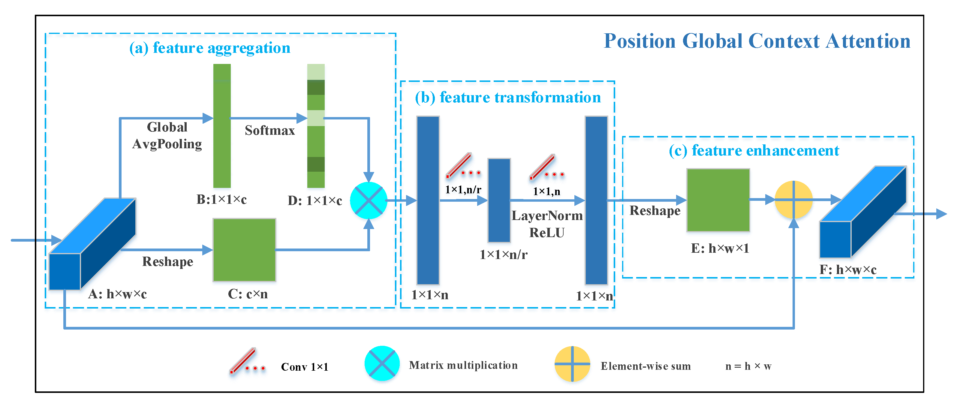
In order to alleviate the problems of AMs in the DBMA and the DBDA, we developed two novel AMs known as channel global context (GC) attention and position GC attention inspired by the GC block [34]. The proposed channel GC attention and position GC attention can make full use of global contextual information with less time consumption. In addition, the interactions among enhanced channels or positions are modeled to learn high-level semantic feature representations. Concretely, our channel and position GC attentions can be abstracted into three procedures: (a) feature aggregation, which aggregates the features of all positions or channels via weighted summation under the aid of the channel or position attention map to yield global contextual features; (b) feature transformation, which learns the adaptive channel-wise or position-wise non-linear relationships by a bottleneck transform module consisting of two 1 × 1 convolutions, the ReLU activation function, and layer normalization; (c) feature enhancement, which merges the transformed global contextual information into features of all positions or channels by element-wise summation to capture long-range dependencies and obtain more powerful feature representations. To sum up, the main contributions of this paper are the following:

• An end-to-end spectral-spatial framework with channel and position global context (GC) attention (SSGCA) is proposed for HSI classification. The SSGCA has two branches: the spectral branch with channel GC attention is used to capture spectral features, while the spatial branch with position GC attention is used to obtain spatial features. At the end of the network, spectral and spatial features are combined for HSI classification.
• A channel GC attention and a position GC attention are proposed for feature enhancement in the spectral branch and the spatial branch, respectively. The channel GC attention is designed to capture interactions among channels, while the position GC attention is invented to explore interactions among positions. Both GC attentions can make full use of global contextual information with less time consumption and model long-range dependencies to obtain more powerful feature representations.
• The SSGCA network is applied to three well-known public HSI datasets. Experimental results demonstrate that our network achieves the best performance compared with other well-known networks.

The remainder of this article is organized as follows. Section 2 introduces the related work, and Section 3 describes the proposed methodology in detail. Next, the experimental results and comprehensive analysis are reported in Section 4 and Section 5. Finally, some conclusions of this article are drawn in Section 6.

2. Related Work

In this section, we introduce the related work that plays a significant role in our work, including 3D convolution operation, CNN-based methods for HSI classification, the dense connection block, and the attention mechanism (AM).

2.1. 3D Convolution Operation

The 3D convolution operation was first proposed in [35] to compute features from both spatial and temporal dimensions for human action recognition. Later, various 3D CNN networks based on the 3D convolution operation were designed for HSI classification. For example, Chen et al. [25] proposed a deep 3D CNN model, which employed several 3D convolutional and pooling layers to extract deep spectral-spatial feature maps for classification. Different from [25], Li et al. [36] designed a 3D CNN network, which stacks 3D convolutional layers without the pooling layer to extract deep spectral-spatial-combined features effectively. Furthermore, Roy et al. [26] proposed a hybrid model named HybridSN which consists of 3D CNN based on 3D convolution and 2D CNN based on 2D convolution to facilitate the joint spectral-spatial feature representations and spatial feature representations. To sum up, 1D convolution extracts spectral features, whereas 2D convolution extracts local spatial features; unlike 1D and 2D convolution, 3D convolution allows extracting spatial and spectral information simultaneously.

In this paper, 3D convolution is employed as a fundamental element playing a crucial role in the feature extraction stage. At the same time, BN [37] and the ReLU activation function are attached to each 3D convolution operation in our network, which can accelerate the learning rate of DL models and assist the network to learn non-linear feature relationships, respectively. The 3D convolution operation can be formulated as [35]:

$$v_{li}^{xyz}=g(\sum _j\sum _{h=0}^{H_l-1}\sum _{w=0}^{W_l-1}\sum _{r=0}^{R_l-1}{k}_{lij}^{hwr}{v}_{(l-1)j}^{(x+h)(y+w)(z+r)}+b_{li}),$$

(1)

where l indicates the layer that is discussed, i is the number of feature maps in this layer, $v_{li}^{xyz}$ represents the output at position $(x,y,z)$ on the ith feature maps of the lth layer, $H_l$, $W_l$, and $R_l$ stand for the height, width, and channel number of the 3D convolution kernel, respectively, j indexes the feature maps in the $(l-1)$th layer connected to the current feature maps, $k_{lij}^{hwr}$ is the value at position $(h,w,r)$ of the kernel corresponding to the jth feature maps, g is the activation function, and b is the bias.

2.2. Cube-Based Methods for HSI Classification

Different from traditional pixel-based classification methods [18,19,20] that only utilize spectral information, cube-based methods explore both spectral and spatial information from HSIs. Recently, many cube-based methods were proposed for HSI classification, such as DRCNN [38], CDCNN [39], DCPN [40], and SSAN [41]; these methods have attracted increasing attention and made considerable achievements. In the remainder of this section, we will briefly introduce the process of HSI classification with the aid of cube-based methods.

For a specific pixel of an HSI, a square HSI data cube is cropped, centered on this pixel, which is taken as the input data of the cube-based network, and the land cover label of the HSI cube is determined by its central pixel. Let $x_i\in R^{h\times w\times c}$ represent the ith HSI data cube and $y_i\in \{1,2,\dots ,m\}$ represent the corresponding land cover label, where $h\times w$ is the spatial size, c is the number of channels, and m is the number of land cover categories. Consequently, the ith sample can be denoted as $(x_i,y_i)$, and all samples will be divided into three sets. To be specific, a certain number of samples are randomly selected as the training set; another certain number of samples are randomly assigned as the validation set; and the remaining samples are used as the testing set. The training set is fed into the network in batches to adjust the trainable parameters; the validation set acts as the monitor to observe the optimization process of the network, while the testing set serves to evaluate the classification performance of the network. In this article, the designed network is also cube-based, but the difference is that we introduce AMs into our network to enhance the extracted features and thus obtain more powerful feature representations for HSI classification.

2.3. Dense Connection Block

In order to alleviate the vanishing gradient problem, strengthen feature propagation, and encourage feature reuse, Gao et al. [29] designed DenseNet, which introduces direct connections from any layer to all subsequent layers. Inspired by SSRN [28] and DenseNet, Wang et al. [30] proposed the FDSSC network for HSI classification to learn discriminative spectral and spatial features separately. The FDSSC consists of a spectral dense block, a reducing dimension block, and a spatial dense block. In the DBMA [31] and DBDA [32], the capability to extract features of dense connection blocks from the FDSSC was demonstrated once again. For this article, we also use the spectral dense block and spatial dense block from the FDSSC as the baseline network for feature extraction, and the difference is that the spectral and spatial branches are connected in parallel, the same as the DBMA and DBDA, rather than in a cascaded manner. These two dense connection blocks can reduce the high dimensionality and automatically learn more effective spatial and spectral features separately with little depletion of the computing resources.

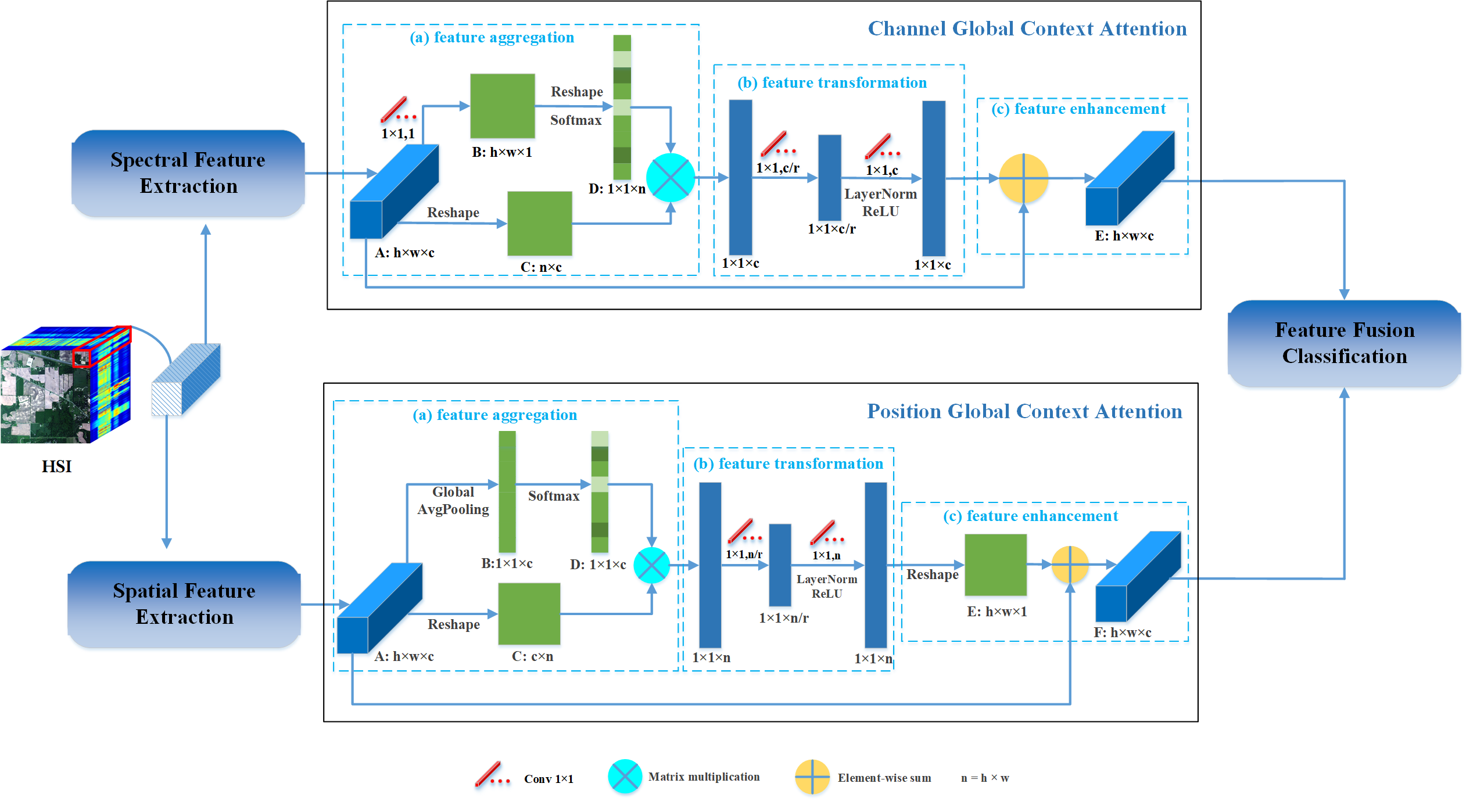
As shown in Figure 1 and Figure 2, the spectral and spatial dense blocks consist of several sets of feature maps, direct connections, and 3D convolution operations. The BN operation and the ReLU activation function are also included. In the spectral dense block, the size of the 3D convolution kernels is $(1\times 1\times d,k)$, the stride is $(1,1,1)$, and the manner of padding is “same”, which can ensure the output shape is the same as the input shape. The feature maps of the lth layer receive feature maps from all previous outputs and the initial input. Consequently, if we set $x_l$ as the lth feature maps, we can calculate it by the previous $(l-1)$ feature maps, as shown in the following equation:

$$x_l=H_l[x_0,x_1,\dots ,x_{l-1}],$$

(2)

where $[x_0,x_1,\dots ,x_{l-1}]$ refers to the concatenation of the previous feature maps. $H_l(·)$ includes batch normalization (BN), the ReLU activation function, and 3D convolution operations. Furthermore, the number of lth input feature maps $k_l$ can be calculated as follows:

$$k_l=k_0+(l-1)\times k,$$

(3)

where $k_0$ is the number of initial feature maps and k is the kernel number of the 3D convolution operation. In this paper, the spectral dense block consists of four layers; if the input shape is $(p\times p\times b,k_0)$, after the above analysis, we can know that the shape of the output remains $(p\times p\times b)$, and the channel number will change to $k_0+3\times k$.

In the spatial dense block, the kernel size of 3D convolution is $(r\times r\times 1,k)$, the manner of padding is “same”, and the stride is $(1,1,1)$. Same as spectral dense block, the feature maps of current layer have been linked to previous feature maps and back feature maps, and the final output is merged by all previous outputs and the initial input. As shown in Figure 2, if the input shape is $(q\times q\times m,k_0)$, the shape of output feature maps remain $(q\times q\times m)$ and the channel number will change into $k_0+3\times k$ after spatial dense block.

2.4. Attention Mechanism

Different spectral channel and spatial position features acquired by the DL-based network may provide different contributions to classification. Therefore, how to make models focus on the most informative part and differentiate low-correlation information is essential for classification. The AM was firstly presented in language translation [42]. Immediately afterwards, it developed rapidly and acquired incredible breakthroughs in the field of computer vision. For example, Hu et al. [43] invented a squeeze-and-excitation network (SENet) to adaptively refine the channel-wise feature response by modeling interdependencies among channels, which brings significant improvements to the performance of CNNs. Different from SENet, Woo et al. [44] proposed a convolutional block attention module (CBAM), which exploits attention in both the channel and position dimensions to learn what and where to emphasize or suppress, aiming at refining intermediate features effectively. With the purpose of capturing long-range dependencies, Wang et al. [45] presented non-local operations as a generic family of building blocks for capturing long-range dependencies, which compute the response at a position as a weighted sum of the features at all positions. Inspired by the non-local block from [45] and the SE block from [43], Yue Cao et al. [34] proposed a global context (GC) block, which is lightweight and can model the global context more effectively.

Recently, AMs have received increasing attention in the field of remote sensing. Since HSIs contain more abundant information, especially in the spectral dimension, it is critical to avoid the impact of redundant information while utilizing useful information efficiently. Therefore, plenty of DL-based methods combined with various kinds of AMs have been designed for HSI classification, such as SSAN [41], the DBMA [31], the DBDA [32], and so on. These networks further improved the classification performance with the assistance of AMs; however, previous AMs attached to CNN-based networks for HSI classification have some insufficiencies. For example, they inadequately utilize global contextual information and cannot model long-range dependencies effectively; in addition, they are time-consuming and cannot learn non-linear feature relationships. To tackle these issues, the GC block [34] employed in the field of general images seems to work. However, the GC block only focuses on the channel dimension, and in the HSI data cube, the position characteristics also play a crucial role in classification. Therefore, we invented a position-wise framework resembling the GC block, aiming at processing the position information of HSIs. These two frameworks called channel GC attention and position GC attention are attached to the spectral and spatial branch to optimize the features, avoiding the disadvantages of previous AMs. The implementation details of our channel GC attention and position GC attention are described in Section 3.1 and Section 3.2.

3. Methodology

In this Section, we introduce the general architecture of the proposed channel global context (GC) attention and position GC attention. We describe the implementation details of our spectral-spatial network with channel and position GC attention (SSGCA) in three specific stages.

3.1. Channel Global Context Attention

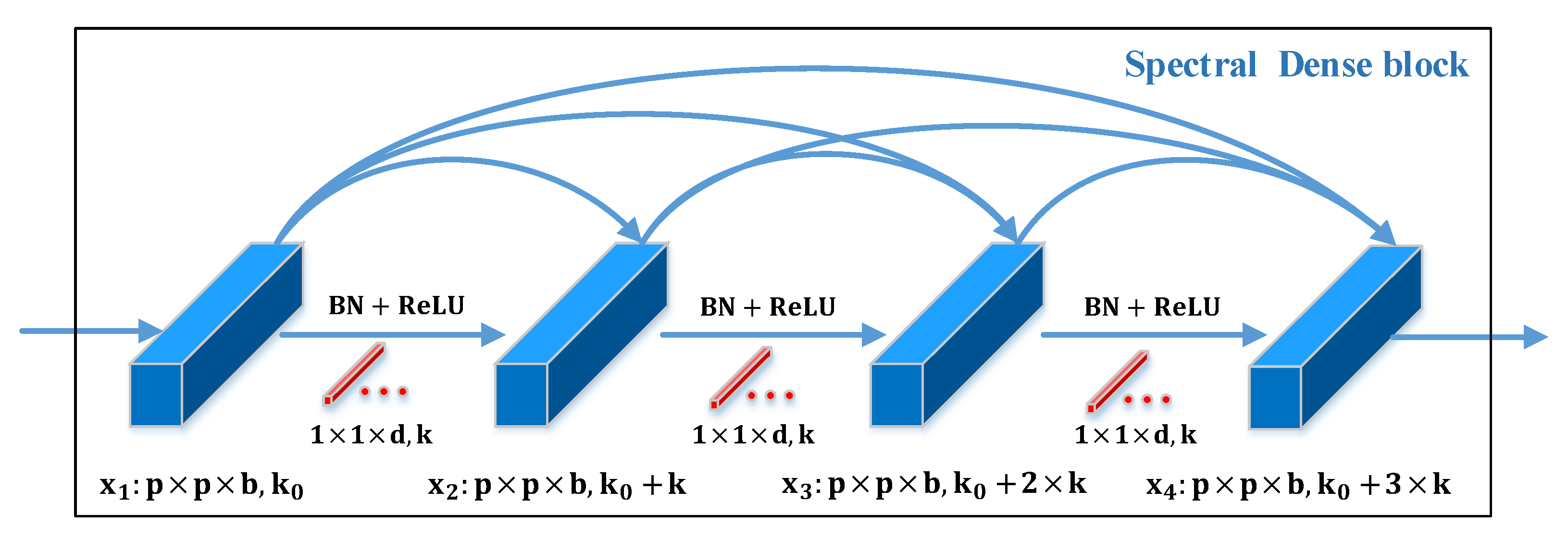
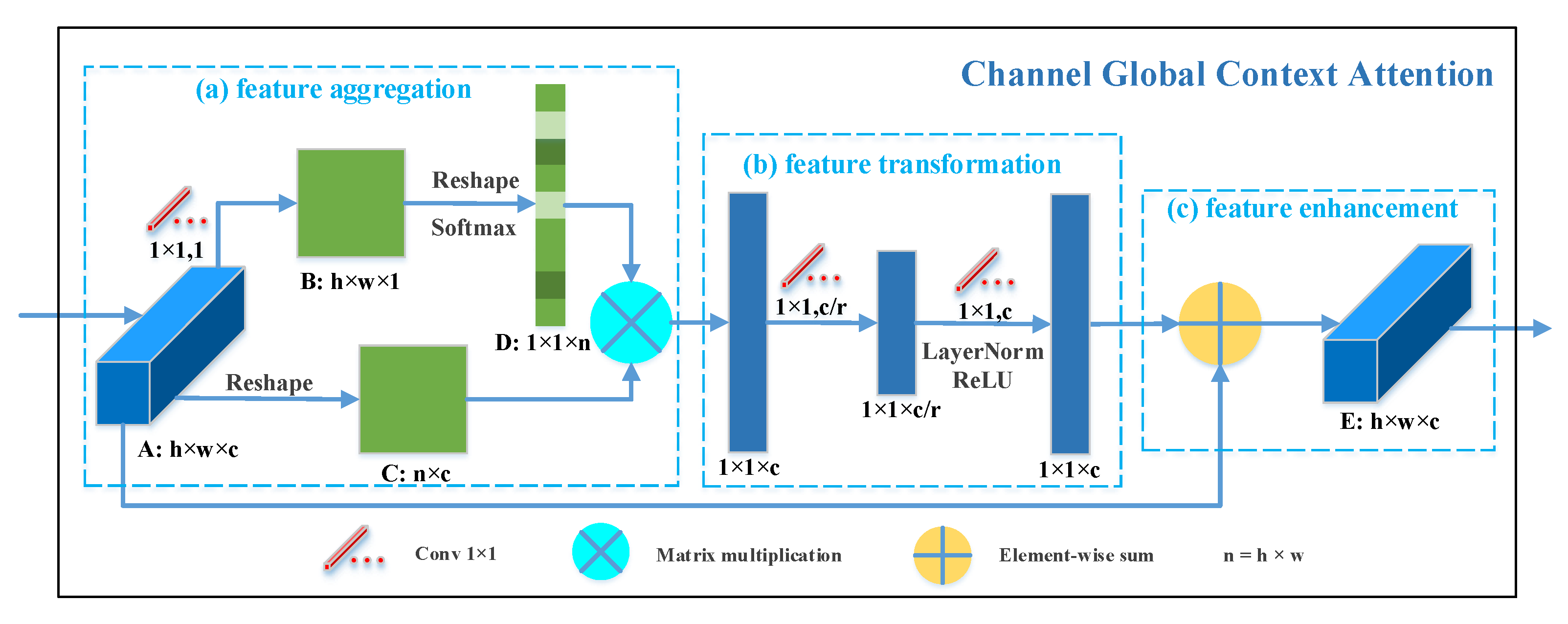
As illustrated in Figure 3, the channel GC attention is abstracted into three procedures: (a) feature aggregation, which performs a weighted summation on the features of all positions to yield global contextual features; (b) feature transformation, which learns nonlinear channel-wise inner relationships by a bottleneck transform module; (c) feature enhancement, which merges the transformed channel features into each position to utilize long-range dependencies, optimizing the feature representations. Specifically, for the input feature maps $A\in R^{h\times w\times c}$, we first feed it into a $1\times 1$ convolutional layer of which the kernel number is 1, and a new feature map $B\in R^{h\times w\times 1}$ is obtained. Then, B is reshaped to $R^{1\times 1\times n}$, and a softmax operation is applied to it to obtain the attention map $D\in R^{1\times 1\times n}$, where $n=h\times w$. Meanwhile, A is reshaped to $C\in R^{n\times c}$. After that, we conduct a matrix multiplication between C and the attention map D to obtain channel features that contain global contextual position information. Next, the channel features are fed into a bottleneck transform module to learn nonlinear interactions between channels. The bottleneck transform module consists of two $1\times 1$ convolutional layers, a ReLU activation function between them, and a layer normalization operation (LN) [46] before the ReLU to benefit optimization. The bottleneck ratio r is selected from {8, 12, 16, 20} (this parameter is discussed in Section 5.2) to reduce the computational cost and prevent overfitting. Finally, we perform an element-wise sum operation between transformed features and initial input features A to get the final output $E\in R^{h\times w\times c}$.

Above all, our channel GC attention can be defined as:

$$p_i^{{}^{\prime }}=p_i+f(\sum _{j=1}^{N_p}{\alpha }_j·p_j),$$

(4)

where p and $p^{\prime }$ are the input and output feature maps of the channel GC attention, respectively, $i\in \{1,2,\dots ,N_p\}$ is the index of the positions, and $N_p=h\times w$ is the number of positions. ${\sum }_{j=1}^{N_p}{\alpha }_j·p_j$ represents the global contextual features aggregated from all positions via weighted summation with weight ${\alpha }_j$. The weight ${\alpha }_j$ is calculated according to:

$${\alpha }_j=\frac{exp\left(W_u{p}_j\right)}{{\sum }_{m=1}^{N_p}exp\left(W_u{p}_m\right)},$$

(5)

where $W_u$ denotes the linear transformation matrix. $f(·)$ denotes the feature transformation operations in the bottleneck transform module, shown as:

$$f(·)=W_{v2}ReLU\left(LN\left(W_{v1}(·)\right)\right),$$

(6)

which includes two linear transformation matrices $W_{v1}$ and $W_{v2}$, a layer normalization, and a ReLU activation function.

3.2. Position Global Context Attention

As illustrated in Figure 4, the position GC attention is also described as three procedures: (a) feature aggregation, which applies a weighted summation among features of all channels to generate global contextual features; (b) feature transformation, which aims to learn the nonlinear inner relationships between position features by a bottleneck transform module; (c) feature enhancement, which captures long-range dependencies to form better feature representations by merging the transformed position features into each channel. Concretely, as shown in Figure 4, the input feature maps is $A\in R^{h\times w\times c}$. First, a global average pooling is applied on A to squeeze global spatial information into a feature vector $B\in R^{1\times 1\times c}$; meanwhile, A is reshaped to $C\in R^{c\times n}$. Then, B is fed into a softmax layer to obtain attention map $D\in R^{1\times 1\times c}$. After that, a matrix multiplication is performed on attention map D and matrix C, where the result is the position features, which include global contextual channel information. The same as the channel GC attention, the position features are fed into a bottleneck transform module to learn nonlinear position-wise interactions, and the value of bottleneck ratio r is the same as that of the channel GC attention. Finally, we reshape the output of transform module to $E\in R^{h\times w\times 1}$ and execute an element-wise sum operation between A and E to obtain the final output $F\in R^{h\times w\times c}$.

Likewise, our position GC attention can be defined as:

$$c_i^{{}^{\prime }}=c_i+\delta (\sum _{j=1}^{N_c}{b}_j·c_j),$$

(7)

where c and $c^{\prime }$ denote the input and output feature maps of the position GC attention, respectively, $i\in \{1,2,\dots ,N_c\}$ is the index of channels, and $N_c$ is the number of channels. ${\sum }_{j=1}^{N_c}{b}_j·c_j$ represents the global contextual features aggregated from all channels via weighted summation with weight $b_j$. The weight $b_j$ is calculated from Equation (8), in which $F_{avg}$ represents a global average pooling operation. $\delta (·)$ denotes the operations of the bottleneck transform module formulated as Equation (9), where $W_{k1}$ and $W_{k2}$ are also linear transformation matrices.

$$b_j=\frac{exp\left(F_{avg}\left(c_j\right)\right)}{{\sum }_{m=1}^{N_c}exp\left(F_{avg}\left(c_m\right)\right)},$$

(8)

$$\delta (·)=W_{k2}ReLU\left(LN\left(W_{k1}(·)\right)\right).$$

(9)

3.3. Spectral-Spatial Network with Global Context Attention

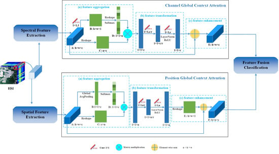
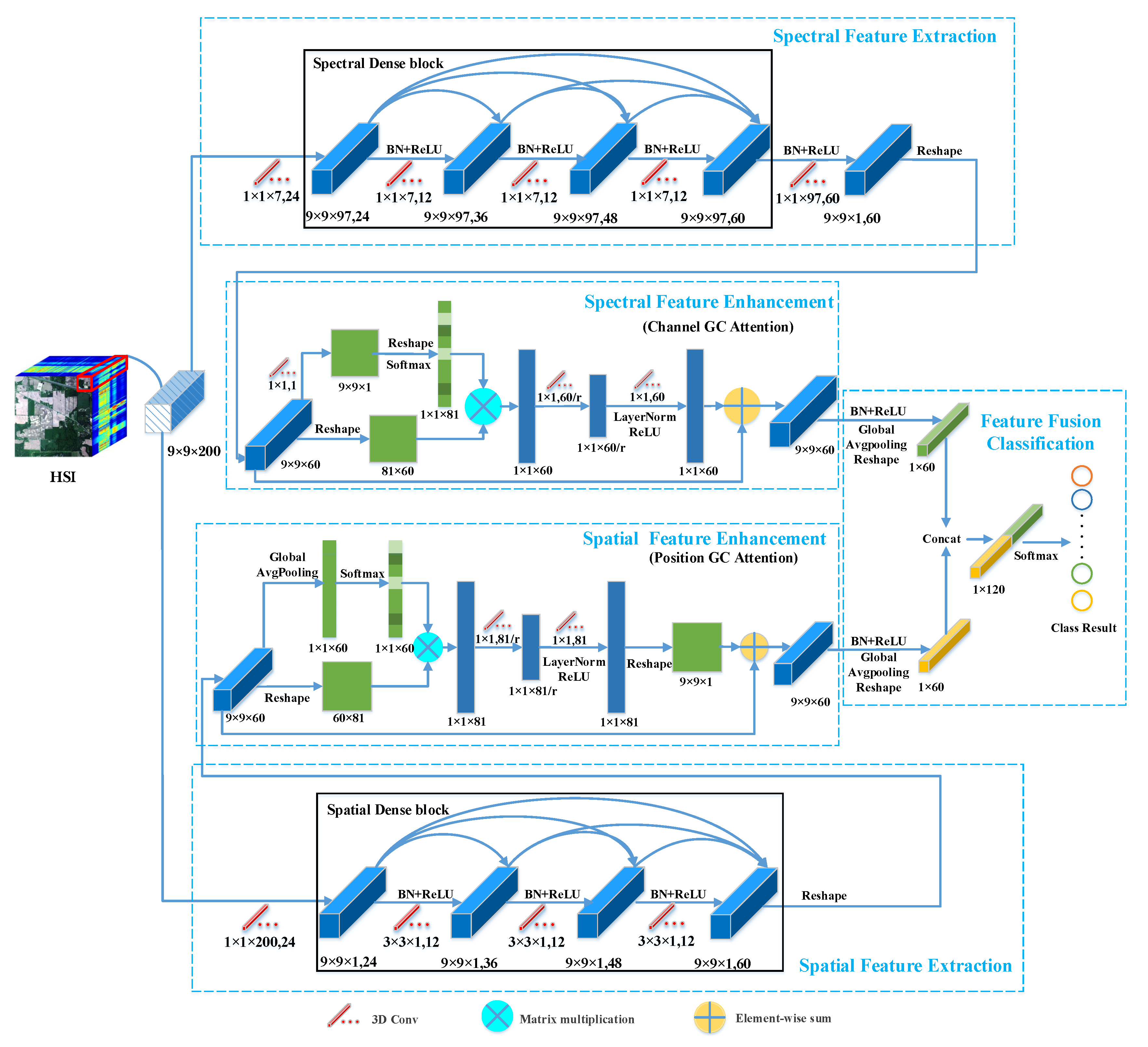
The proposed SSGCA consists of three parts: feature extraction, feature enhancement, and feature fusion classification. Feature extraction focuses on collecting discriminative spectral and spatial features based on dense connection blocks. Feature enhancement pays close attention to obtaining more powerful feature representations via GC attentions. Feature fusion classification concatenates spectral and spatial features directly to determine the final land cover categories. Next, we take the Indian Pines dataset as an example to introduce the network structure of these three stages.

3.3.1. Feature Extraction

As shown in Figure 5, this part consists of two parallel stages: spectral feature extraction stage and spatial feature extraction stage. The former stage aims to extract spectral features, while the latter is to explore spatial information. For each pixel to be classified, a corresponding HSI data cube of size $(9\times 9\times 200)$ is cropped for both the spectral and spatial branches. In the spectral branch, a 3D convolution is first applied to reduce the number of bands. The kernel size is $(1\times 1\times 7,24)$; the stride is $(1,1,2)$; and the padding is “valid”. After that, the feature maps with the shape of $(9\times 9\times 97,24)$ are generated. Then, they are fed into the spectral dense block, in which the kernel size, padding, and stride of 3D convolution are all $(1\times 1\times 7,12)$, “same”, and $(1,1,1)$. As a result, the shape of feature maps changes into $(9\times 9\times 97,60)$, and they are re-imported to a 3D convolution layer with a kernel size of $(1\times 1\times 97,60)$ and a padding manner of “valid” to reduce the number of channels again. Consequently, the final feature maps of the spectral feature extraction stage can be obtained, and the shape is $(9\times 9\times 1,60)$. Similar to the spectral branch, in the spatial branch, the input data cube is first fed into a 3D convolution layer, and the kernel size, stride, and padding are $(1\times 1\times 200,24)$, $(1,1,1)$, and “valid”. Then, the output feature maps are fed into the spatial dense block, in which the kernel size, stride, and padding of 3D convolution are all $(3\times 3\times 1,12)$, $(1,1,1)$, and “same”. After that, the final output of the spatial feature extraction stage with the size of $(9\times 9\times 1,60)$ is acquired. The use of the ReLU activation function and the BN operation can be seen in Figure 5. In addition, the detailed descriptions of the spectral dense block and the spatial dense block are shown in Section 2.3, and the implementation details of feature extraction are described in

Table 1. The implementation details of the spectral feature extraction stage.

Input Size	Layer Operations	Output Size
$(9\times 9\times 200)$	Conv3D$(1\times 1\times 7,24)$	$(9\times 9\times 97,24)$
$(9\times 9\times 97,24)$	BN-ReLU-Conv3D$(1\times 1\times 7,12)$	$(9\times 9\times 97,12)$
$(9\times 9\times 97,24)/(9\times 9\times 97,12)$	Concatenate	$(9\times 9\times 97,36)$
$(9\times 9\times 97,36)$	BN-ReLU-Conv3D$(1\times 1\times 7,12)$	$(9\times 9\times 97,12)$
$(9\times 9\times 97,24)/(9\times 9\times 97,12)/(9\times 9\times 97,12)$	Concatenate	$(9\times 9\times 97,48)$
$(9\times 9\times 97,48)$	BN-ReLU-Conv3D$(1\times 1\times 7,12)$	$(9\times 9\times 97,12)$
$(9\times 9\times 97,24)/(9\times 9\times 97,12)/(9\times 9\times 97,12)/(9\times 9\times 97,12)$	Concatenate	$(9\times 9\times 97,60)$
$(9\times 9\times 97,60)$	BN-ReLU-Conv3D$(1\times 1\times 97,60)$	$(9\times 9\times 1,60)$

and

Table 2. The implementation details of the spatial feature extraction stage.

Input Size	Layer Operations	Output Size
$(9\times 9\times 200)$	Conv3D$(1\times 1\times 200,24)$	$(9\times 9\times 1,24)$
$(9\times 9\times 1,24)$	BN-ReLU-Conv3D$(3\times 3\times 1,12)$	$(9\times 9\times 1,12)$
$(9\times 9\times 1,24)/(9\times 9\times 1,12)$	Concatenate	$(9\times 9\times 1,36)$
$(9\times 9\times 1,36)$	BN-ReLU-Conv3D$(3\times 3\times 1,12)$	$(9\times 9\times 1,12)$
$(9\times 9\times 1,24)/(9\times 9\times 1,12)/(9\times 9\times 1,12)$	Concatenate	$(9\times 9\times 1,48)$
$(9\times 9\times 1,48)$	BN-ReLU-Conv3D$(3\times 3\times 1,12)$	$(9\times 9\times 1,12)$
$(9\times 9\times 1,24)/(9\times 9\times 1,12)/(9\times 9\times 1,12)/(9\times 9\times 1,12)$	Concatenate	$(9\times 9\times 1,60)$

.

3.3.2. Feature Enhancement

After the feature extraction stage, spectral feature maps with abundant spectral signatures and spatial feature maps with plentiful spatial information can be acquired. Then, these two type of features will be fed into spectral and spatial feature enhancement stage, as shown in Figure 5, respectively. The spectral feature enhancement stage serves to capture interactions between channels via the channel GC attention, while the spatial feature enhancement stage aims to explore position relationships by the position GC attention. Both GC attentions can make full use of global contextual information, learn nonlinear feature interrelationships, and adequately capture long-range dependencies. As described in Figure 5, the extracted spectral and spatial feature maps are first reshaped to $(9\times 9\times 60)$ and then separately fed into the GC attention module. Both the input size and output size of the channel GC attention and the position GC attention are $(9\times 9\times 60)$. Detailed descriptions of GC attentions are displayed in Section 3.1 and Section 3.2, and the implementation details of the feature enhancement stage are reported in

Table 3. The implementation details of the spectral feature enhancement stage.

Input Size	Layer Operations	Output Size
$(9\times 9\times 60)$	Conv2D$(1\times 1,1)$	$(9\times 9\times 1)$
$(9\times 9\times 1)$	Reshape	$(1\times 1\times 81)$
$(1\times 1\times 81)$	Softmax	$(1\times 1\times 81)$
$(9\times 9\times 60)$	Reshape	$(81\times 60)$
$(1\times 1\times 81)/(81\times 60)$	Matrix Multiplication	$(1\times 1\times 60)$
$(1\times 1\times 60)$	Conv2D$(1\times 1,60/r)$	$(1\times 1\times 60/r)$
$(1\times 1\times 60/r)$	LayerNorm/ReLU	$(1\times 1\times 60/r)$
$(1\times 1\times 60/r)$	Conv2D$(1\times 1,60)$	$(1\times 1\times 60)$
$(1\times 1\times 60)/(9\times 9\times 60)$	Element-wise Sum	$(9\times 9\times 60)$

and

Table 4. The implementation details of the spatial feature enhancement stage.

Input Size	Layer Operations	Output Size
$(9\times 9\times 60)$	Global Average Pooling	$(1\times 1\times 60)$
$(1\times 1\times 60)$	Softmax	$(1\times 1\times 60)$
$(9\times 9\times 60)$	Reshape	$(60\times 81)$
$(1\times 1\times 60)/(60\times 81)$	Matrix Multiplication	$(1\times 1\times 81)$
$(1\times 1\times 81)$	Conv2D$(1\times 1\times 81/r)$	$(1\times 1\times 81/r)$
$(1\times 1\times 81/r)$	LayerNorm/ReLU	$(1\times 1\times 81/r)$
$(1\times 1\times 81/r)$	Conv2D$(1\times 1,81)$	$(1\times 1\times 81)$
$(1\times 1\times 81)$	Reshape	$(9\times 9\times 1)$
$(9\times 9\times 1)/(9\times 9\times 60)$	Element-wise Sum	$(9\times 9\times 60)$

.

3.3.3. Feature Fusion Classification

The transformed spectral and spatial features yielded by the feature enhancement stages are separately fed into a global average pooling layer and a reshape layer to aggregate information in each channel, and as a result, both the size of the spectral and spatial feature maps are from $(9\times 9\times 60)$ to $(1\times 60)$. Finally, we perform a concatenation between these two feature maps and feed the result to a fully-connected layer with the softmax activation function to obtain the certain land cover label. The implementation details of the feature fusion classification stage are shown in

Table 5. The implementation details of the feature fusion classification stage.

Input Size	Layer Operations	Output Size
$(9\times 9\times 60)$	Global Average Pooling/Reshape	$(1\times 60)$
$(9\times 9\times 60)$	Global Average Pooling/Reshape	$(1\times 60)$
$(1\times 60)/(1\times 60)$	Concatenate	$(1\times 120)$
$(1\times 120)$	FC with Softmax	$(1\times ClassNum)$

.

4. Experiments

4.1. Datasets

In this paper, we selected three well-known HSI datasets to evaluate the effectiveness of our network compared with other widely used methods proposed before. The selected datasets include Indian Pines (IN), University of Pavia (UP), and the Salinas Valley (SV) dataset.

The IN dataset was captured by the Airborne Visible/Infrared Imaging Spectrometer (AVIRIS) over the Indian Pines test site in northwestern Indiana in 1992, and the image contains 16 vegetation classes and has $(145\times 145)$ pixels with a spatial resolution of 20 m per pixel. After removing 20 water absorption bands, this dataset includes 200 spectral bands for analysis ranging from 400 to 2500 nm.

The UP dataset was acquired over the city of Pavia, Italy, in 2002 by an airborne instrument—the Reflective Optics Spectrographic Imaging System (ROSIS). This dataset consists of $(640\times 340)$ pixels with a 1.3 m per pixel spatial resolution and 103 spectral bands ranging from 430 to 860 nm after removing 12 noisy bands. The dataset contains a large number of background pixels, so the total number of pixels including the features is only 42,776. There are 9 types of features, including asphalt roads, bricks, pastures, trees, bare soil, etc.

The SV dataset was also gathered by the AVIRIS sensor over the region of Salinas Valley, CA, USA, with a 3.7 m per pixel spatial resolution. The same as the IN dataset, twenty water absorption bands of the SV dataset were discarded. After that, the SV dataset consisted of 204 spectral bands and $(512\times 217)$ pixels for analysis from 400 to 2500 nm. The dataset presents 16 classes related to vegetables, vineyard fields, and bare soil.

In this paper, we randomly selected a few samples of each dataset for training and validation. To be specific, from the IN dataset, we selected 5% of the samples for training and 5% for validation. For the UP dataset, we selected 1% of the samples for training and 1% for validation. In addition, we also selected 1% as training samples and 1% as validation samples from the SV dataset.

Table 6. The samples for each category of training, validation, and testing for the Indian Pines (IN) dataset.

Number	Class	Total	Train	Val	Test
1	Alfalfa	46	3	3	40
2	Corn-notill	1428	71	71	1286
3	Corn-mintill	830	41	41	748
4	Corn	237	11	11	215
5	Grass-pasture	483	24	24	435
6	Grass-trees	730	36	36	658
7	Grass-pasture-mowed	28	3	3	22
8	Hay-windrowed	478	23	23	432
9	Oats	20	3	3	14
10	Soybean-notill	972	48	48	876
11	Soybean-mintill	2455	122	122	2211
12	Soybean-clean	593	29	29	535
13	Wheat	205	10	10	185
14	Woods	1265	63	63	1139
15	Buildings-Grass-Trees-Drives	386	19	19	348
16	Stone-Steel-Towers	93	4	4	85
Total		10,249	510	510	9229

,

Table 7. The samples for each category of training, validation, and testing for the University of Pavia (UP) dataset.

Number	Class	Total	Train	Val	Test
1	Asphalt	6631	66	66	6499
2	Meadows	18,649	186	186	18,277
3	Gravel	2099	20	20	2059
4	Trees	3064	30	30	3004
5	Painted metal sheets	1345	13	13	1319
6	Bare Soil	5029	50	50	4929
7	Bitumen	1330	13	13	1304
8	Self-Blocking Bricks	3682	36	36	3610
9	Shadows	947	9	9	929
Total		42,776	423	423	41,930

and

Table 8. The samples for each category of training, validation and testing for the Salinas Valley (SV) dataset.

Number	Class	Total	Train	Val	Test
1	Broccoli_green_weeds_1	2009	20	20	1969
2	Broccoli_green_weeds_2	3726	37	37	3652
3	Fallow	1976	19	19	1938
4	Fallow_rough_plow	1394	13	13	1368
5	Fallow_smooth	2678	26	26	2626
6	Stubble	3959	39	39	3881
7	Celery	3579	35	35	3509
8	Grapes_untrained	11,271	112	112	11,047
9	Soil_vineyard_develop	6203	62	62	6079
10	Corn_senesced_green_weeds	3278	32	32	3214
11	Lettuce_romaine_4wk	1068	10	10	1048
12	Lettuce_romaine_5wk	1927	19	19	1889
13	Lettuce_romaine_6wk	916	9	9	898
14	Lettuce_romaine_7wk	1070	10	10	1050
15	Vineyard_untrained	7268	72	72	7124
16	Vineyard_vertical_trellis	1807	18	18	1771
Total		54,129	533	533	53,063

list the sample numbers for the training, validation, and testing for the three datasets.

4.2. Evaluation Measures

In order to quantify the performance of the proposed method, four evaluation metrics were selected: the accuracy of each class, the overall accuracy (OA), the average accuracy (AA), and the kappa coefficient. The OA is the ratio of the number of correctly classified HSI pixels to the total number of HSI pixels in the testing samples. The AA is the mean of the accuracies for different land cover categories. Kappa measures the consistency between the classification results and the ground truth. Let $M\in R^{(m\times n)}$ represent the confusion matrix of the classification results, where m denotes the number of land cover categories. The values of the OA, AA, and kappa can be calculated as follows [47]:

$$OA=sum\left(diag\right(M\left)\right)/sum\left(M\right),$$

(10)

$$AA=mean\left(\right(diag\left(M\right)./\left(sum\right(M,2\left)\right),$$

(11)

$$Kappa=\frac{OA-(sum(M,1)\times sum(M,2))/{\left(sum\left(M\right)\right)}^2}{1-(sum(M,1)\times sum(M,2))/{\left(sum\left(M\right)\right)}^2},$$

(12)

where $diag\left(M\right)\in R^{m\times 1}$ is a vector of the diagonal elements of M, $sum(·)\in R^1$ represents the sum of all elements of the matrix, $sum(·,1)\in R^{1\times m}$ represents the sum of the elements in each column, $sum(·,2)\in R^{m\times 1}$ represents the sum of the elements in each row, $mean(·)\in R^1$ represents the mean of all elements, and $./$ represents the element-wise division.

4.3. Experimental Setting

In this paper, SVM with the RBF kernel [48] and several well-known DL-based methods were selected for comparison, including SSRN [28], the FDSSC [30], the DBMA [31], and the DBDA [32]. To ensure the fairness of the comparative experiments, we adopted the same hyperparameter settings for these methods, and all experiments were executed on an NVIDIA GeForce GTX 2070 SUPER GPU with a memory of 32 GB. For the DL-based methods, the spatial size of the HSI cubes was set to $9\times 9$, the batch size was 64, and the number of training epochs was set to 200. Besides, a cross-entropy loss function was exploited to measure the difference between the predicted value and the real value to train the parameters of the networks, which can be formulated as follows:

$$Loss=-\sum _{j=1}^m{y}_{j}log\left(p_j\right),$$

(13)

where m is the number of land cover categories, $y_j$ denotes the land cover label (if the category is j, $y_j$ is 1; otherwise, $y_j$ equals to 0), and $p_j$ represents the probability that the category is j, which is calculated by the softmax function. To prevent overfitting, the early stopping strategy was adopted. If the loss value of the validation dataset no longer decreases for 20 epochs, the training process will be stopped. Furthermore, the optimizer was set to Adam with a 0.001 learning rate, and we used the cosine annealing [49] method to dynamically adjust the learning rate, which can prevent the model from falling into local minima. The learning rate was adjusted according to the following equation [32,49]:

$${\eta }_t={\eta }_{min}^i+\frac{1}{2}({\eta }_{max}^i-{\eta }_{min}^i)(1+cos\left(\frac{T_{cur}}{T_i}\pi \right)),$$

(14)

where ${\eta }_t$ is the learning rate within the ith run and $[{\eta }_{max}^i-{\eta }_{min}^i]$ is the range of the learning rate. $T_{cur}$ represents the count of epochs that were executed, and $T_i$ controls the count of epochs that will be executed in a cycle of adjustment. Finally, a dropout layer was adopted in the bottleneck transform module of GC attentions to further avoid overfitting, and the dropout percentage p was set to $0.5$.

4.4. Classification Results

Table 9. The classification results for the IN dataset with $5\%$ training samples.

Number	Class	SVM	SSRN	FDSSC	DBMA	DBDA	SSGCA
1	Alfalfa	32.56	100.00	92.50	43.90	97.56	97.62
2	Corn-notill	74.21	96.19	92.29	97.36	95.49	98.37
3	Corn-mintill	57.03	88.96	90.34	99.59	89.71	95.28
4	Corn	24.34	88.68	96.70	86.70	95.77	99.52
5	Grass-pasture	84.31	92.15	99.77	91.82	91.90	98.16
6	Grass-trees	96.83	98.16	99.54	99.85	98.63	99.54
7	Grass-pasture-mowed	88.00	95.83	100.00	100.00	100.00	95.24
8	Hay-windrowed	89.67	97.71	100.00	100.00	100.00	100.00
9	Oats	41.18	100.00	76.47	70.59	100.00	100.00
10	Soybean-notill	66.02	89.23	97.37	96.93	95.46	93.96
11	Soybean-mintill	78.18	97.51	91.37	97.25	99.05	98.69
12	Soybean-clean	50.53	97.32	98.71	95.51	97.96	98.30
13	Wheat	91.28	98.91	100.00	100.00	100.00	100.00
14	Woods	94.01	99.21	100.00	96.21	99.47	99.82
15	Buildings-Grass-Trees-Drives	45.78	92.90	95.13	100.00	99.43	98.57
16	Stone-Steel-Towers	69.66	91.57	96.47	86.05	89.41	95.24
OA(%)		74.74	95.45	96.18	96.78	96.99	98.13
AA(%)		67.72	95.27	95.79	91.36	96.87	98.02
Kappa×100		70.97	94.81	95.65	96.33	96.57	97.86

,

Table 10. The classification results for the UP dataset with 1% training samples.

Number	Class	SVM	SSRN	FDSSC	DBMA	DBDA	SSGCA
1	Asphalt	91.94	99.22	98.35	98.60	99.43	100.00
2	Meadows	98.49	99.52	99.98	99.99	98.76	99.56
3	Gravel	61.81	47.98	98.39	88.49	99.17	92.65
4	Trees	80.39	97.44	93.55	96.77	96.83	95.97
5	Painted metal sheets	99.02	99.85	100.00	99.62	99.55	100.00
6	Bare Soil	66.38	99.31	99.63	96.43	99.98	100.00
7	Bitumen	69.17	97.02	100.00	86.91	97.62	99.77
8	Self-Blocking Bricks	83.71	99.70	95.74	94.13	88.85	98.97
9	Shadows	99.57	99.35	99.46	95.59	97.84	98.16
OA(%)		88.46	96.72	98.77	97.54	98.00	99.02
AA(%)		83.39	93.26	98.35	95.17	97.56	98.34
Kappa×100		84.38	95.64	98.37	96.73	97.36	98.71

and

Table 11. The classification results for the SV dataset with 1% training samples.

Number	Class	SVM	SSRN	FDSSC	DBMA	DBDA	SSGCA
1	Broccoli_green_weeds_1	99.35	99.54	100.00	100.00	100.00	100.00
2	Broccoli_green_weeds_2	99.16	99.12	100.00	100.00	100.00	100.00
3	Fallow	94.17	98.20	100.00	100.00	99.33	99.38
4	Fallow_rough_plow	98.41	87.84	99.71	99.27	99.12	99.56
5	Fallow_smooth	97.02	98.78	99.73	98.70	99.47	98.02
6	Stubble	99.62	100.00	99.56	100.00	100.00	100.00
7	Celery	99.44	99.80	100.00	99.91	99.97	99.97
8	Grapes_untrained	81.41	93.41	98.48	99.52	91.18	95.76
9	Soil_vineyard_develop	99.23	99.80	100.00	100.00	100.00	100.00
10	Corn_senesced_green_weeds	83.30	97.20	95.74	97.29	99.31	98.66
11	Lettuce_romaine_4wk	90.74	99.52	100.00	99.90	100.00	99.81
12	Lettuce_romaine_5wk	99.00	100.00	99.95	99.95	99.79	100.00
13	Lettuce_romaine_6wk	97.24	99.78	99.22	99.11	96.97	100.00
14	Lettuce_romaine_7wk	92.74	99.52	99.05	99.33	98.39	99.14
15	Vineyard_untrained	56.43	94.08	91.74	91.74	97.21	99.23
16	Vineyard_vertical_trellis	89.99	96.26	100.00	99.49	99.21	97.47
OA(%)		87.89	96.97	98.23	98.49	97.56	98.69
AA(%)		92.33	97.68	98.95	99.01	98.75	99.19
Kappa×100		86.48	96.63	98.03	98.32	97.28	98.54

show the OAs, AAs, kappa coefficients, and classification accuracies of each class for the three HSI datasets. Obviously, the proposed method SSGCA achieves the best OAs, AAs, and kappa coefficients compared with the other methods on the three HSI datasets, which can demonstrate the effectiveness and generalizability of our method. For example, when 5% of the samples are randomly selected for training on the IN dataset, our method achieves the best accuracy with 98.13% OA, improving 1.14% over the DBDA (96.99%), 1.35% over the DBMA (96.78%), 1.95% over the FDSSC (96.18%), and 2.68% over SSRN (95.45%). In contrast to SVM (74.74%), our method achieves a considerable improvement of more than 23% in terms of OA. Besides, from the results, we can learn that all the DL-based methods achieve higher performance than SVM on three HSI datasets. For example, the OAs of the DL-based methods obtain more than a 20% increase in contrast to SVM on the IN dataset and about a 10% increase on the UP and SV dataset. The reason is that DL-based methods can exploit high-level, abstract, and discriminative feature representations to improve the classification performance.

Furthermore, the classification results of the FDSSC, DBMA, and DBDA on the three datasets are higher than those of SSRN with approximately a 1–2% improvement in OA. These results demonstrate the effectiveness of a dense connection structure, which is adopted in the FDSSC, DBMA, and DBDA. Moreover, comparing the FDSSC to the three attention-based methods, we can find that the proposed SSGCA achieves a higher OA than the FDSSC for all three datasets; however, the results of the DBMA and DBDA are not always higher than those of the FDSSC. For instance, the OA of the DBDA is lower than the FDSSC on the UP and SV datasets, and the OA of the DBMA is below the FDSSC on the UP dataset. This means that our GC attentions can optimize the feature representations more effectively compared with the AMs in the DBMA and DBDA when these three methods employ the same feature extraction network. The reason is that our GC attentions can utilize global contextual information adequately, capture feature interactions well, and model long-range dependencies effectively. Finally, from the classification accuracies of each class for the three HSI datasets, we can find that our SSGCA achieves more stable results, benefiting from the invented GC attentions. Taking the SV dataset as an example, the best and worst single-category results of the SSGCA are 100% and 95.76%, respectively, with a difference of only 4.24%, while the difference is 8.82% for the DBDA (best: 100%; worst: 91.18%), 8.26% for the DBMA and FDSSC (best: 100%; worst: 91.74%), 12.16% for SSRN (best: 100%; worst: 87.84%), and 43.19% for SVM (best: 99.62%; worst: 56.43%).

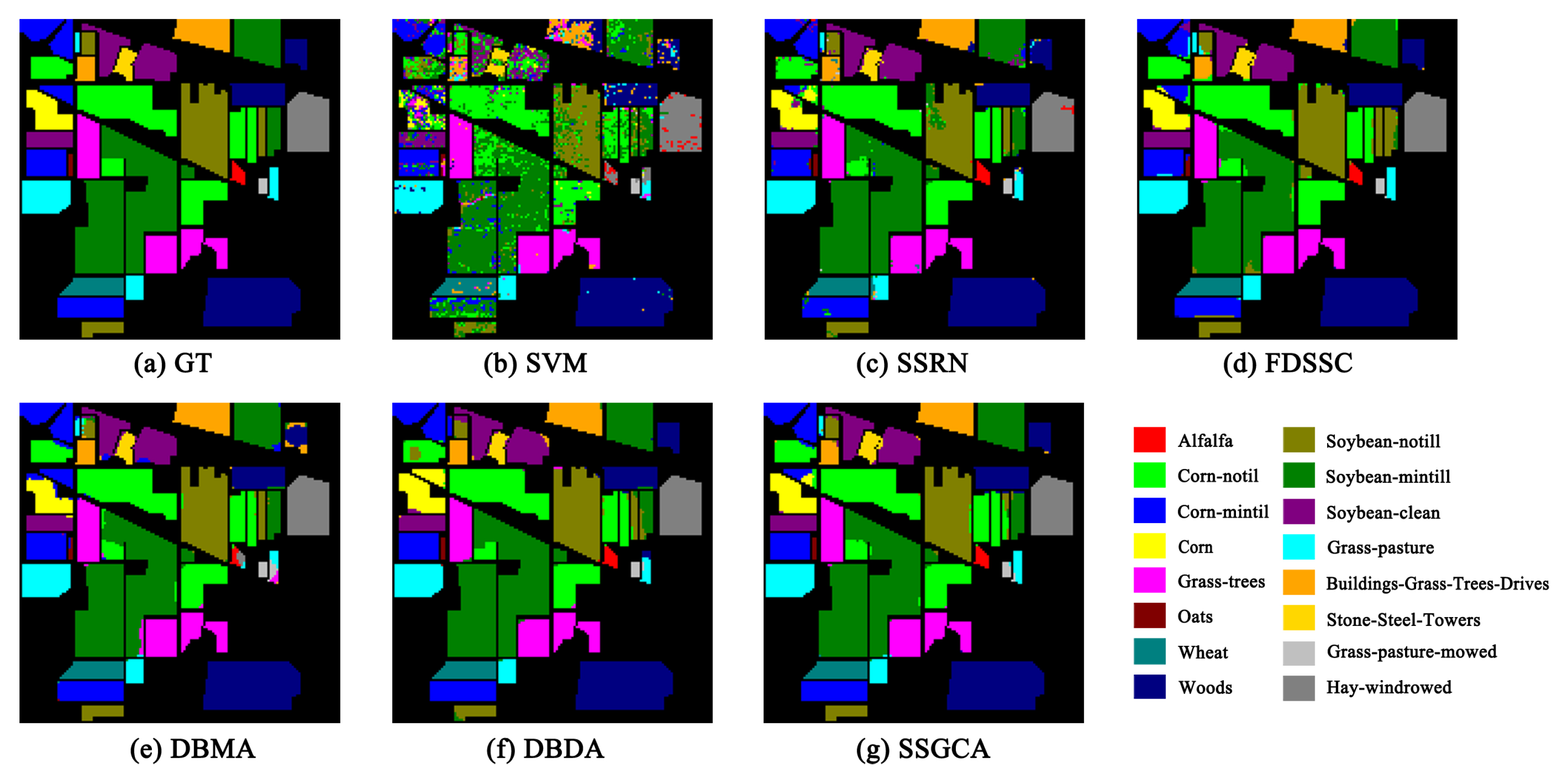
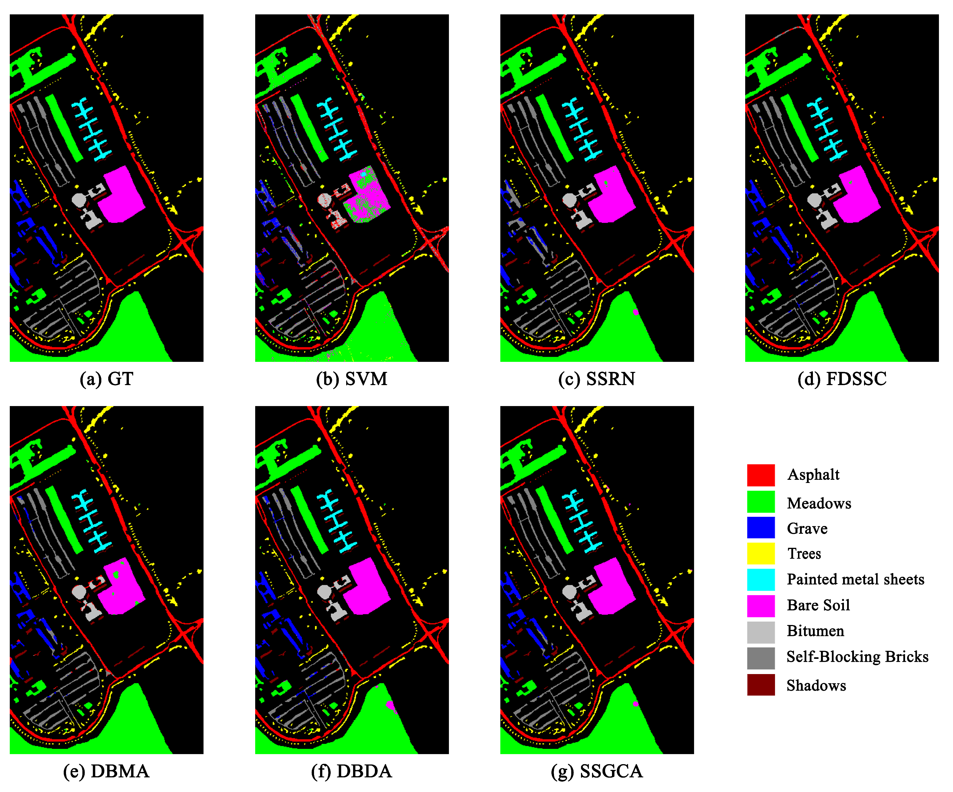
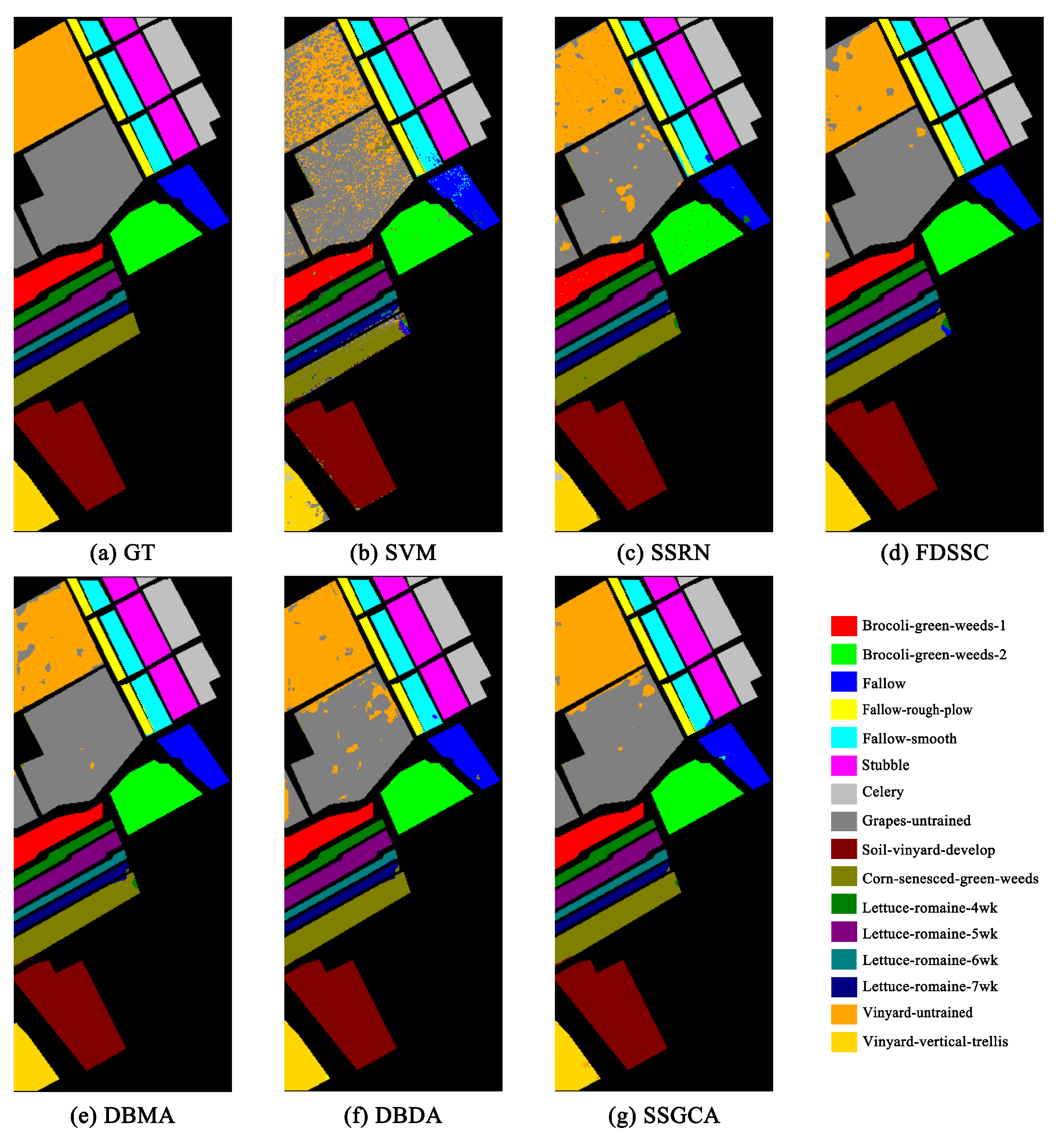
Figure 6, Figure 7 and Figure 8 show the visualization maps of all methods along with the corresponding ground truth maps for the three HSI datasets. Firstly, from the visual classification results, we can intuitively conclude that the proposed SSGCA delivers the most accurate and smooth classification maps on all datasets, because the SSGCA can obtained more powerful feature representations with the aid of our GC attentions for classification. Secondly, compared to DL-based methods, the classification maps of SVM on the three datasets show plenty of mislabeled areas due to the lack of incorporation of spatial neighborhood information, and the extracted features are at a low-level. Thirdly, we can find that the visual classification maps of the attention-based methods are smoother than SSRN and the FDSSC, especially at the edges of land cover areas, and it can be observed that the SSGCA yields better classification maps in contrast to the DBDA and DBMA, because our GC attentions can adequately utilize global contextual information, learn nonlinear feature interactions, and model long range dependencies for feature enhancing compared with the attentions in the DBDA and DBMA.

5. Other Investigations

In this section, we conduct further investigations in the following three aspects. Firstly, different proportions of training samples from the three datasets are selected for all methods to investigate the performance of our method with different training sample numbers. Secondly, several ablation experiments are designed to investigate the effectiveness of our channel GC attention and position GC attention; meanwhile, we explore the effectiveness of different bottleneck ratio values in GC attentions. Thirdly, we report the total trainable parameter number and running time of all methods to investigate the computational efficiency of different methods.

5.1. Investigation of the Proportion of Training Samples

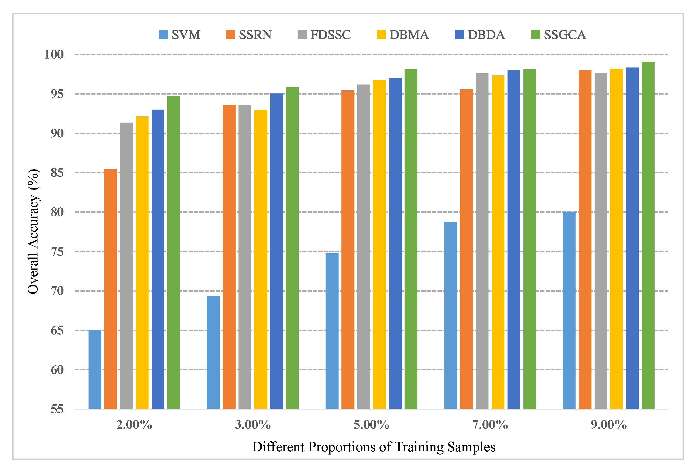
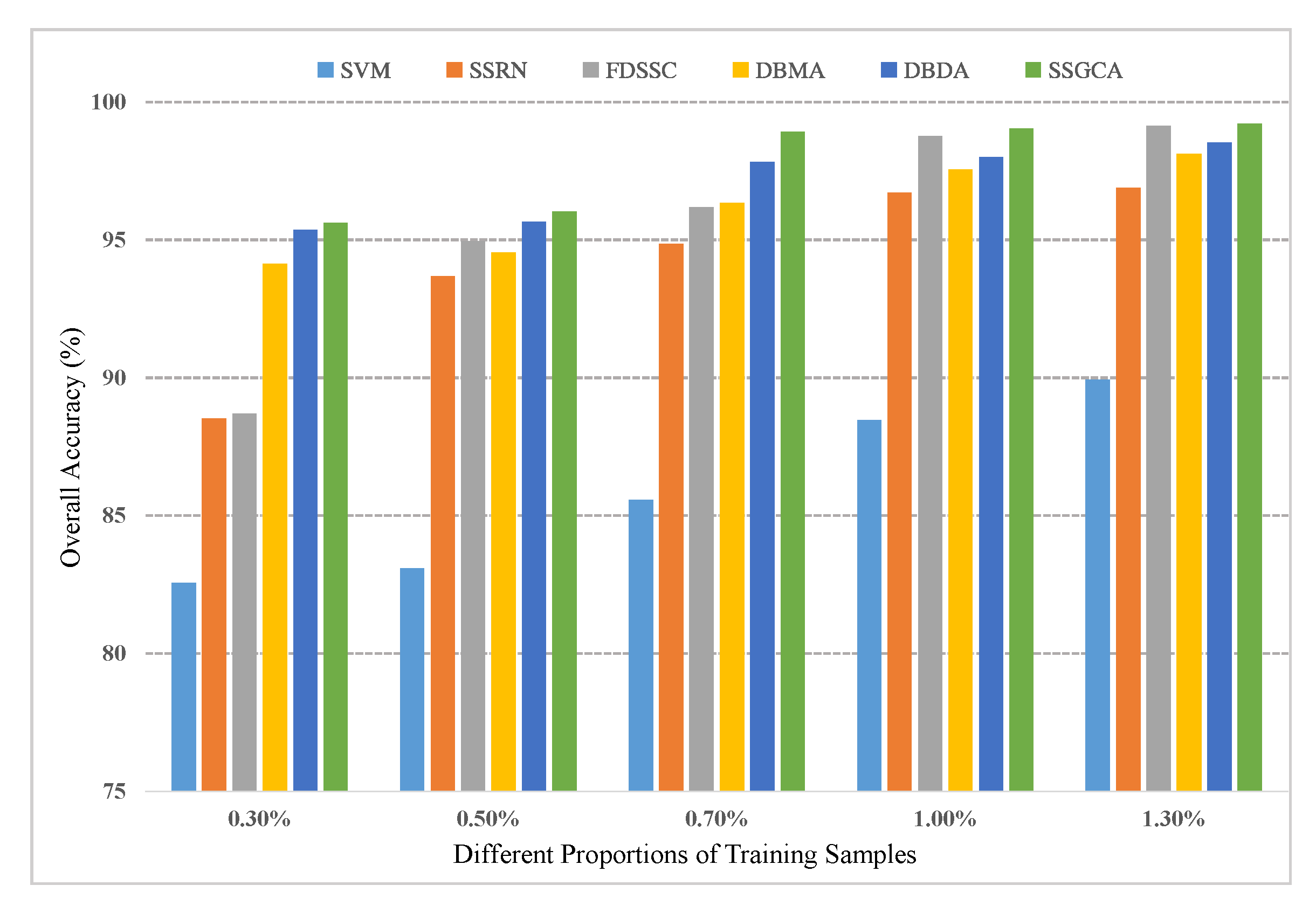
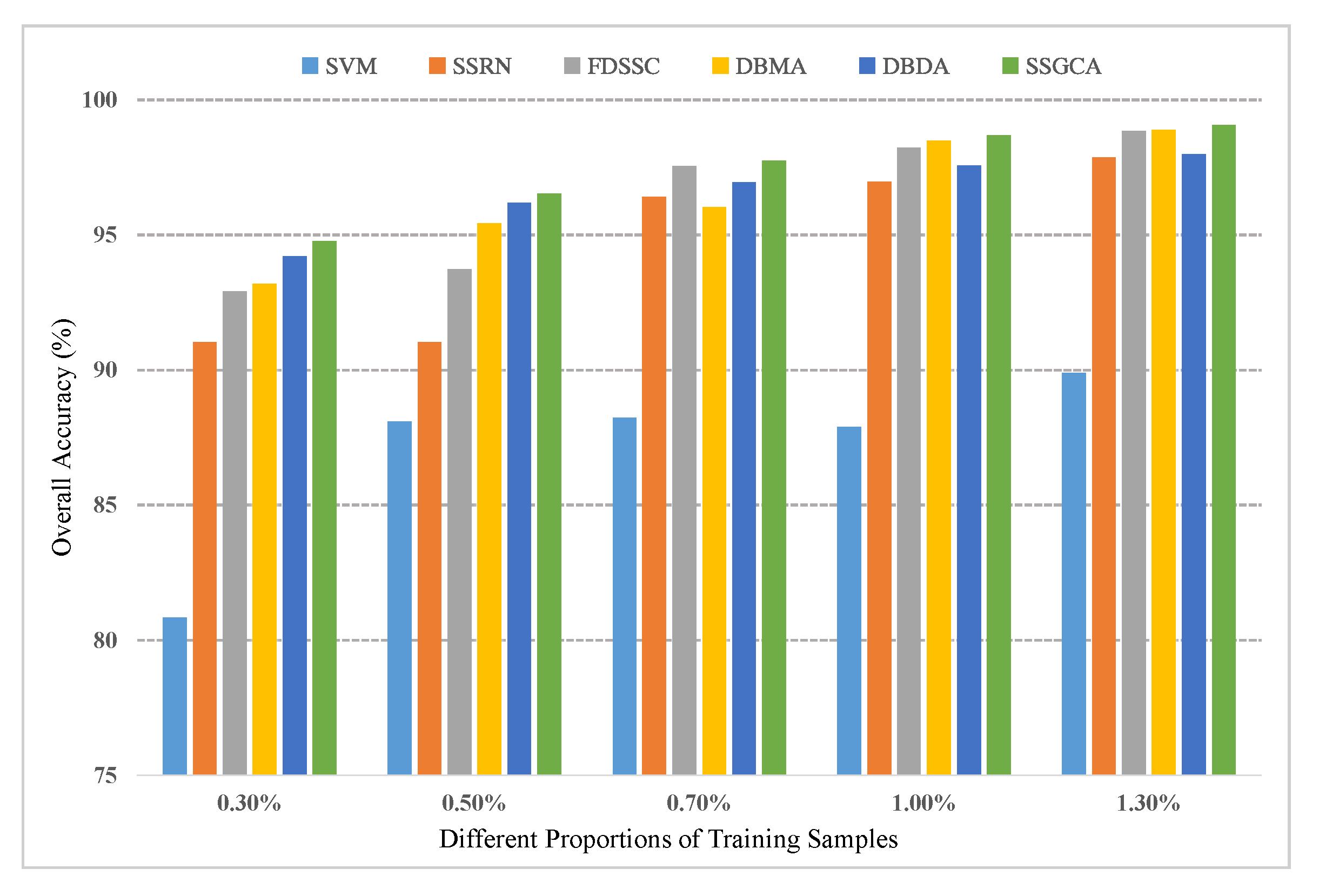
In this part, several experiments are designed to explore the robustness and generalizability of the proposed method with different training proportions. On the one hand, two percent, 3%, 7%, and 9% training samples were randomly selected from the IN dataset; on the other hand, zero-point-three percent, 0.5%, 0.7%, and 1.3% training samples were randomly selected from the UP and SV datasets. Figure 9, Figure 10 and Figure 11 display the results for the different training ratios of the six methods on the three datasets.

Firstly, it is evident that different numbers of training samples bring about different classification performances for all methods: as the number of training samples increases, the classification accuracy increases, and the proposed method SSGCA achieves the best performance compared with other methods with different numbers of training samples on the three datasets. Secondly, the performance of the FDSSC is relatively poor when the training set is quite small compared to the DBMA, DBDA, and SSGCA, but as the training samples increase, the FDSSC outperforms the DBMA and DBDA, while the classification accuracy is closer to the best result, especially on the UP and SV datasets. From this comparison, we can learn that AMs have a more significant effect when lacking training samples. Thirdly, we can see that the accuracies of the DL-based methods get closer along with the increasing of the training samples, particularly on the IN and SV datasets.

5.2. Investigation of the Global Context Attentions

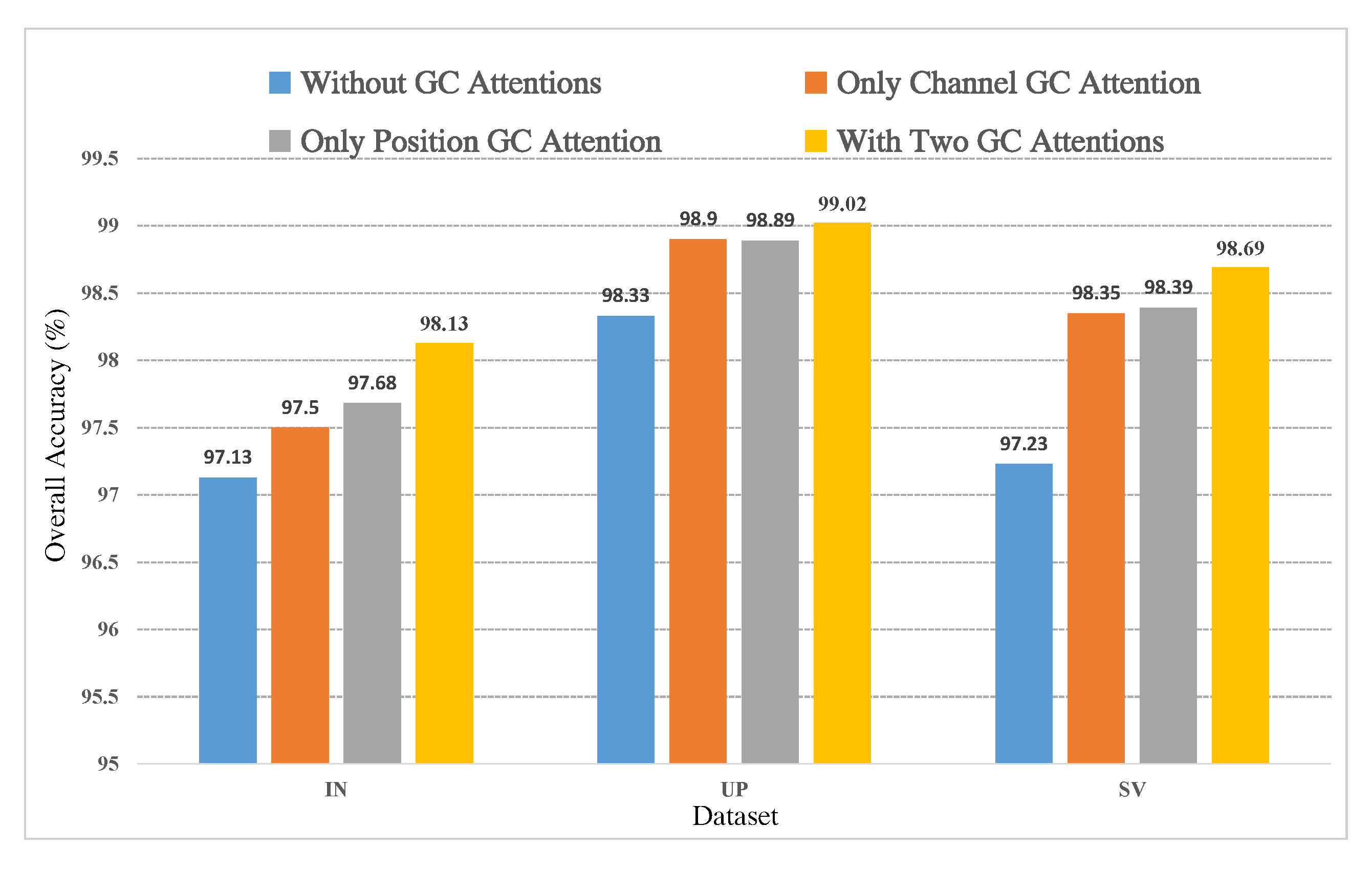
In this part, several ablation experiments are executed to demonstrate the effectiveness of the GC attentions in this article, including experiments only with the channel GC attention, experiments only with the position GC attention, and experiments without GC attentions. The training sample proportions of IN, UP, and SV in these experiments were 5%, 1%, and 1%, respectively, and the bottleneck ratio r was set to 16. It can be observed from Figure 12 that both GC attentions can improve the classification performance on each dataset. For example, on the IN dataset, the channel GC attention brings an improvement of 0.37% OA, the position GC attention brings an improvement of 0.55% OA, and using both GC attentions can improve by 1% OA, which is a considerable advance in the case of limited training samples and high baseline accuracy. In addition, we can find that the channel GC attention plays a more significant role compared with the position GC attention on the IN and SV datasets, and the result is opposite on the UP dataset; however, the highest results can be achieved when both GC attentions are included in our network for all three datasets.

The bottleneck ratio r introduced in Section 3.1 and Section 3.2 is a hyperparameter, which aims to reduce the computational cost of our GC attentions. In this part, we also designed several experiments to explore the effectiveness of different values of the bottleneck ratio. The training sample proportions of IN, UP, and SV selected in these experiments were 5%, 1%, and 1%, respectively. The classification results reported in

Table 12. The classification results at different bottleneck ratios on the three datasets.

Ratio r	IN	UP	SV
8	97.17	98.54	98.44
12	97.88	98.88	97.84
16	98.13	99.02	98.69
20	97.85	98.74	97.46

show that our SSGCA network acquires the highest performance when the bottleneck ratio r is set to 16 on the three datasets.

5.3. Investigation on Running Time

Table 13. The number of parameters and the running time of different methods on the IN dataset.

Dataset	Method	Total Params	Training (s)	Testing (s)
	SVM	-	48.02	1.39
	SSRN	364,168	661.90	3.87
IN	FDSSC	1,227,490	1,573.78	4.86
	DBMA	610,031	170.32	5.90
	DBDA	382,326	128.97	5.56
	SSGCA	379,208	104.17	4.25

,

Table 14. The number of parameters and the running time of different methods on the UP dataset.

Dataset	Method	Total Params	Training (s)	Testing (s)
	SVM	-	9.51	3.36
	SSRN	216,537	304.39	9.38
UP	FDSSC	651,063	930.75	11.92
	DBMA	330,376	73.59	14.22
	DBDA	206,351	35.44	13.42
	SSGCA	203,233	33.40	10.32

and

Table 15. The number of parameters and the running time of different methods on the SV dataset.

Dataset	Method	Total Params	Training (s)	Testing (s)
	SVM	-	26.19	6.39
	SSRN	370,312	536.83	22.54
SV	FDSSC	1,251,490	1,277.54	28.48
	DBMA	621,647	408.68	34.59
	DBDA	389,622	151.05	32.72
	SSGCA	386,504	118.34	24.95

report the total number of trainable parameters of the DL-based methods. From the results, we can find that the SSGCA has fewer trainable parameters than the FDSSC, DBMA, and DBDA. Meanwhile, Table 13, Table 14 and Table 15 show the training time and test time of all methods on the three datasets. Note that all experiments’ results were collected when the training sample proportions were 5%, 1%, and 1% on IN, UP, and SV, respectively, and the bottleneck ratio r of the SSGCA was set to 16. From these three tables, we can learn that SVM consumes less training and testing time than the DL-based methods. Furthermore, the proposed SSGCA spends the least training time and the second least testing time among all DL-based methods on the three datasets. Above all, we can conclude that the proposed SSGCA obtains the best classification performance with little time consumption, which can prove the high efficiency of our method.

6. Conclusions

In this article, an end-to-end spectral-spatial network with channel and position global context (GC) attention (SSGCA) is proposed for HSI classification. The proposed SSGCA is based on the work of many predecessors, including 3D convolution, DenseNet, the FDSSC, GCNet, the DBDA, and so on. The SSGCA mainly contains three stages: feature extraction, feature enhancement, and feature fusion classification. Feature extraction is based on dense connection blocks to acquire discriminative spectral and spatial features in two separate branches. Feature enhancement aims to optimize spectral and spatial feature representations to improve the classification performance by the channel GC attention and the position GC attention, respectively. Compared to the previous AMs used in HSI classification methods, our GC attentions can make full use of global contextual information and capture adaptive nonlinear feature relationships in the spectral and spatial dimensions with less computation consumption. Furthermore, our AMs can adequately model long-range dependencies. Feature fusion classification concatenates two types of features in the channel dimension, then the fusion features are fed into an FC layer with the softmax function to generate the final land cover category. Moreover, we designed a great quantity of experiments on three public HSI datasets to verify the effectiveness, generalizability, and robustness of our method. Later, analyses on the experimental results demonstrated that the proposed method acquired the best performance compared to other well-known methods. In the future, we will combine our GC attention with other DL-based networks and apply these novel models on other HSI datasets.

References

- Masoud, M.; Bahram, S.; Mohammad, R.; Fariba, M.; Yun, Z. Very Deep Convolutional Neural Networks for Complex Land Cover Mapping Using Multispectral Remote Sensing Imagery. Remote Sens. 2018, 10, 1119. [Google Scholar]
- Ma, W.; Xiong, Y.; Wu, Y.; Yang, H.; Zhang, X.; Jiao, L. Change Detection in Remote Sensing Images Based on Image Mapping and a Deep Capsule Network. Remote Sens. 2019, 11, 626. [Google Scholar] [CrossRef] [Green Version]
- Ma, W.; Guo, Q.; Wu, Y.; Zhao, W.; Zhang, X.; Jiao, L. A Novel Multi-Model Decision Fusion Network for Object Detection in Remote Sensing Images. Remote Sens. 2019, 11, 737. [Google Scholar] [CrossRef] [Green Version]
- Borana, S.L.; Yadav, S.K.; Parihar, S.K. Hyperspectral Data Analysis for Arid Vegetation Species : Smart & Sustainable Growth. In Proceedings of the 2019 International Conference on Computing, Communication, and Intelligent Systems (ICCCIS), Greater Noida, India, 18–19 October 2019; pp. 495–500. [Google Scholar]
- Luo, F.; Du, B.; Zhang, L.; Zhang, L.; Tao, D. Feature Learning Using Spatial-Spectral Hypergraph Discriminant Analysis for Hyperspectral Image. IEEE Trans. Cybern. 2019, 49, 2406–2419. [Google Scholar] [CrossRef] [PubMed]
- Zhu, M.; Jiao, L.; Liu, F.; Yang, S.; Wang, J. Residual Spectral-Spatial Attention Network for Hyperspectral Image Classification. IEEE Trans. Geosci. Remote Sens. 2020, 59, 449–462. [Google Scholar] [CrossRef]
- Wang, D.; Du, B.; Zhang, L.; Xu, Y. Adaptive Spectral-Spatial Multiscale Contextual Feature Extraction for Hyperspectral Image Classification. IEEE Trans. Geosci. Remote Sens. 2020, 1–17. [Google Scholar] [CrossRef]
- Li, S.; Song, W.; Fang, L.; Chen, Y.; Benediktsson, J.A. Deep Learning for Hyperspectral Image Classification: An Overview. IEEE Trans. Geosci. Remote Sens. 2019, 57, 6690–6709. [Google Scholar] [CrossRef] [Green Version]
- Ma, L.; Crawford, M.M.; Tian, J. Local Manifold Learning-Based k -Nearest-Neighbor for Hyperspectral Image Classification. IEEE Trans. Geosci. Remote Sens. 2010, 48, 4099–4109. [Google Scholar] [CrossRef]
- Li, J.; Bioucas-Dias, J.M.; Plaza, A. Semisupervised Hyperspectral Image Segmentation Using Multinomial Logistic Regression with Active Learning. IEEE Trans. Geosci. Remote Sens. 2010, 48, 4085–4098. [Google Scholar] [CrossRef] [Green Version]
- Bandos, T.V.; Bruzzone, L.; Camps-Valls, G. Classification of Hyperspectral Images with Regularized Linear Discriminant Analysis. IEEE Trans. Geosci. Remote Sens. 2009, 47, 862–873. [Google Scholar] [CrossRef]
- Fauvel, M.; Chanussot, J.; Benediktsson, J.A.; Sveinsson, J.R. Spectral and Spatial Classification of Hyperspectral Data Using SVMs and Morphological Profiles. IEEE Trans. Geosci. Remote Sens. 2008, 46, 3804–3814. [Google Scholar] [CrossRef] [Green Version]
- Bau, T.C.; Sarkar, S.; Healey, G. Hyperspectral Region Classification Using a Three-Dimensional Gabor Filterbank. IEEE Trans. Geosci. Remote Sens. 2010, 48, 3457–3464. [Google Scholar] [CrossRef]
- Zhang, B.; Li, S.; Jia, X.; Gao, L.; Peng, M. Adaptive Markov Random Field Approach for Classification of Hyperspectral Imagery. IEEE Geosci. Remote Sens. Lett. 2011, 8, 973–977. [Google Scholar] [CrossRef]
- Szegedy, C.; Vanhoucke, V.; Ioffe, S.; Shlens, J.; Wojna, Z. Rethinking the Inception Architecture for Computer Vision. In Proceedings of the IEEE Conference on Computer Vision and Pattern Recognition, Las Vegas, NV, USA, 26 June–1 July 2016; pp. 2818–2826. [Google Scholar]
- Long, J.; Shelhamer, E.; Darrell, T. Fully Convolutional Networks for Semantic Segmentation. IEEE Trans. Pattern Anal. Mach. Intell. 2015, 39, 640–651. [Google Scholar]
- Ren, S.; He, K.; Girshick, R.; Sun, J. Faster R-CNN: Towards Real-Time Object Detection with Region Proposal Networks. IEEE Trans. Pattern Anal. Mach. Intell. 2017, 39, 1137–1149. [Google Scholar] [CrossRef] [PubMed] [Green Version]
- Wei, H.; Yangyu, H.; Li, W.; Fan, Z.; Hengchao, L. Deep Convolutional Neural Networks for Hyperspectral Image Classification. J. Sensors 2015, 2015, 1–12. [Google Scholar]
- Mou, L.; Ghamisi, P.; Zhu, X.X. Deep Recurrent Neural Networks for Hyperspectral Image Classification. IEEE Trans. Geosci. Remote Sens. 2017, 55, 3639–3655. [Google Scholar] [CrossRef] [Green Version]
- Li, W.; Wu, G.; Zhang, F.; Du, Q. Hyperspectral Image Classification Using Deep Pixel-Pair Features. IEEE Trans. Geosci. Remote Sens. 2017, 55, 844–853. [Google Scholar] [CrossRef]
- Zhan, Y.; Hu, D.; Wang, Y.; Yu, X. Semisupervised Hyperspectral Image Classification Based on Generative Adversarial Networks. IEEE Geosci. Remote Sens. Lett. 2018, 15, 212–216. [Google Scholar] [CrossRef]
- Bioucas-Dias, J.M.; Plaza, A.; Camps-Valls, G.; Scheunders, P.; Nasrabadi, N.; Chanussot, J. Hyperspectral Remote Sensing Data Analysis and Future Challenges. IEEE Geosci. Remote Sens. Mag. 2013, 1, 6–36. [Google Scholar] [CrossRef] [Green Version]
- He, L.; Li, J.; Liu, C.; Li, S. Recent Advances on Spectral-Spatial Hyperspectral Image Classification: An Overview and New Guidelines. IEEE Trans. Geosci. Remote Sens. 2018, 56, 1579–1597. [Google Scholar] [CrossRef]
- Chen, Y.; Lin, Z.; Zhao, X.; Wang, G.; Gu, Y. Deep Learning-Based Classification of Hyperspectral Data. IEEE J. Sel. Top. Appl. Earth Obs. Remote Sens. 2014, 7, 2094–2107. [Google Scholar] [CrossRef]
- Chen, Y.; Jiang, H.; Li, C.; Jia, X.; Ghamisi, P. Deep Feature Extraction and Classification of Hyperspectral Images Based on Convolutional Neural Networks. IEEE Trans. Geosci. Remote Sens. 2016, 54, 6232–6251. [Google Scholar] [CrossRef] [Green Version]
- Roy, S.K.; Krishna, G.; Dubey, S.R.; Chaudhuri, B.B. HybridSN: Exploring 3D-2D CNN Feature Hierarchy for Hyperspectral Image Classification. IEEE Geosci. Remote Sens. Lett. 2020, 17, 277–281. [Google Scholar] [CrossRef] [Green Version]
- He, K.; Zhang, X.; Ren, S.; Sun, J. Deep Residual Learning for Image Recognition. In Proceedings of the 2016 IEEE Conference on Computer Vision and Pattern Recognition (CVPR), Las Vegas, NV, USA, 26 June–1 July 2016; pp. 770–778. [Google Scholar]
- Zhong, Z.; Li, J.; Luo, Z.; Chapman, M. Spectral-Spatial Residual Network for Hyperspectral Image Classification: A 3-D Deep Learning Framework. IEEE Trans. Geosci. Remote Sens. 2017, 56, 847–858. [Google Scholar] [CrossRef]
- Huang, G.; Liu, Z.; Van Der Maaten, L.; Weinberger, K.Q. Densely Connected Convolutional Networks. In Proceedings of the 2017 IEEE Conference on Computer Vision and Pattern Recognition (CVPR), Honolulu, HI, USA, 21–26 July 2017; pp. 2261–2269. [Google Scholar]
- Wenju, W.; Shuguang, D.; Zhongmin, J.; Liujie, S. A Fast Dense Spectral–Spatial Convolution Network Framework for Hyperspectral Images Classification. Remote Sens. 2018, 10, 1068. [Google Scholar]
- Ma, W.; Yang, Q.; Wu, Y.; Zhao, W.; Zhang, X. Double-Branch Multi-Attention Mechanism Network for Hyperspectral Image Classification. Remote Sens. 2019, 11, 1307. [Google Scholar] [CrossRef] [Green Version]
- Li, R.; Zheng, S.; Duan, C.; Yang, Y.; Wang, X. Classification of Hyperspectral Image Based on Double-Branch Dual-Attention Mechanism Network. Remote Sens. 2020, 12, 582. [Google Scholar] [CrossRef] [Green Version]
- Fu, J.; Liu, J.; Tian, H.; Li, Y.; Bao, Y.; Fang, Z.; Lu, H. Dual Attention Network for Scene Segmentation. In Proceedings of the 2019 IEEE/CVF Conference on Computer Vision and Pattern Recognition (CVPR), Los Angeles, CA, USA, 16–20 June 2019; pp. 3141–3149. [Google Scholar]
- Cao, Y.; Xu, J.; Lin, S.; Wei, F.; Hu, H. GCNet: Non-local Networks Meet Squeeze-Excitation Networks and Beyond. arXiv 2019, arXiv:1904.11492. [Google Scholar]
- Ji, S.; Xu, W.; Yang, M.; Yu, K. 3D Convolutional Neural Networks for Human Action Recognition. IEEE Trans. Pattern Anal. Mach. Intell. 2013, 35, 221–231. [Google Scholar] [CrossRef] [PubMed] [Green Version]
- Ying, L.; Haokui, Z.; Qiang, S. Spectral–Spatial Classification of Hyperspectral Imagery with 3D Convolutional Neural Network. Remote Sens. 2017, 9, 67. [Google Scholar]
- Ioffe, S.; Szegedy, C. Batch Normalization: Accelerating Deep Network Training by Reducing Internal Covariate Shift. In Proceedings of the International Conference on Machine Learning, Lile, France, 6–11 July 2015; Volume 37, pp. 448–456. [Google Scholar]
- Zhang, M.; Li, W.; Du, Q. Diverse Region-Based CNN for Hyperspectral Image Classification. IEEE Trans. Image Process. 2018, 27, 2623–2634. [Google Scholar] [CrossRef] [PubMed]
- Lee, H.; Kwon, H. Going Deeper With Contextual CNN for Hyperspectral Image Classification. IEEE Trans Image Process 2017, 26, 4843–4855. [Google Scholar] [CrossRef] [Green Version]
- Wei, W.; Jinyang, Z.; Lei, Z.; Chunna, T.; Yanning, Z. Deep Cube-Pair Network for Hyperspectral Imagery Classification. Remote Sens. 2018, 10, 783. [Google Scholar] [CrossRef] [Green Version]
- Mei, X.; Pan, E.; Ma, Y.; Dai, X.; Huang, J.; Fan, F.; Du, Q.; Zheng, H.; Ma, J. Spectral-Spatial Attention Networks for Hyperspectral Image Classification. Remote Sens. 2019, 11, 963. [Google Scholar] [CrossRef] [Green Version]
- Bahdanau, D.; Cho, K.; Bengio, Y. Neural Machine Translation by Jointly Learning to Align and Translate. arXiv 2014, arXiv:1409.0473. [Google Scholar]
- Jie, H.; Li, S.; Gang, S.; Albanie, S. Squeeze-and-Excitation Networks. In Proceedings of the IEEE Conference on Computer Vision and Pattern Recognition, Honolulu, HI, USA, 21–26 July 2017; pp. 7132–7141. [Google Scholar]
- Woo, S.; Park, J.; Lee, J.Y.; Kweon, I.S. CBAM: Convolutional Block Attention Module. In Proceedings of the European Conference on Computer Vision (ECCV), Munich, Germany, 8–14 September 2018; pp. 3–19. [Google Scholar]
- Wang, X.; Girshick, R.; Gupta, A.; He, K. Non-local Neural Networks. In Proceedings of the 2018 IEEE/CVF Conference on Computer Vision and Pattern Recognition (CVPR), Salt Lake City, UT, USA, 18–22 June 2018; pp. 7794–7803. [Google Scholar]
- Ba, J.L.; Kiros, J.R.; Hinton, G.E. Layer Normalization. arXiv 2016, arXiv:1607.06450. [Google Scholar]
- Sun, H.; Zheng, X.; Lu, X.; Wu, S. Spectral–Spatial Attention Network for Hyperspectral Image Classification. IEEE Trans. Geosci. Remote Sens. 2020, 58, 3232–3245. [Google Scholar] [CrossRef]
- Melgani, F.; Bruzzone, L. Classification of hyperspectral remote sensing images with support vector machines. IEEE Trans. Geosci. Remote Sens. 2004, 42, 1778–1790. [Google Scholar] [CrossRef] [Green Version]
- Loshchilov, I.; Hutter, F. SGDR: Stochastic Gradient Descent with Restarts. arXiv 2016, arXiv:1608.03983. [Google Scholar]
Figure 1.
The structure of the spectral dense block.
Figure 2.
The structure of spatial dense block.
Figure 3.
The details of the channel global context attention in our network.
Figure 4.
The details of the position global context attention in our network.
Figure 5.
An overview of the spectral-spatial network with channel and position global context attention (SSGCA). This model can be divided into five parts: spectral feature extraction, spectral feature enhancement, spatial feature extraction, spatial feature enhancement, and feature fusion classification.
Figure 6.
Classification maps for the IN dataset with 5% training samples. (a) Ground-truth. (b–g) The classification maps of the corresponding methods.
Figure 7.
Classification maps for the UP dataset with 1% training samples. (a) Ground-truth. (b–g) The classification maps of the corresponding methods.
Figure 8.
Classification maps for the SV dataset with 1% training samples. (a) Ground-truth. (b–g) The classification maps of the corresponding methods.
Figure 9.
Classification results on the IN dataset with different proportions of training samples.
Figure 10.
Classification results on the UP dataset with different proportions of training samples.
Figure 11.
Classification results on the SV dataset with different proportions of training samples.
Figure 12.
The effectiveness of different GC attentions on different datasets.