A Framework for Multi-Dimensional Assessment of Wildfire Disturbance Severity from Remotely Sensed Ecosystem Functioning Attributes

 ,
,  ,
,  and
and
Abstract
:
1. Introduction
2. Materials and Methods
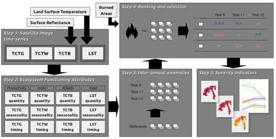
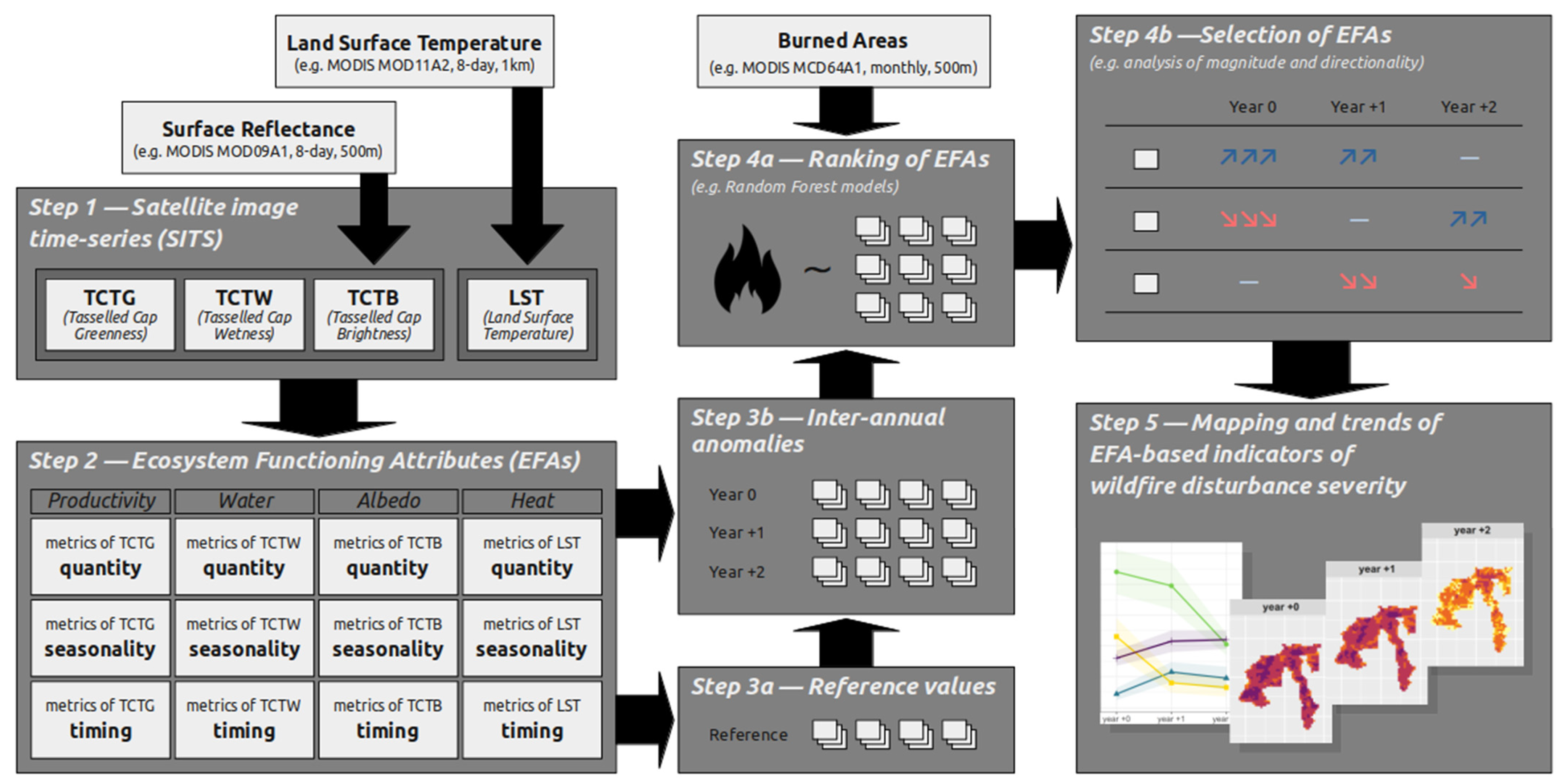
2.1. Generic Framework
2.1.1. General Workflow
2.1.2. Step 1—Satellite Time-Series
2.1.3. Step 2—Extraction of EFAs
2.1.4. Step 3—Computation of EFA Anomalies
2.1.5. Step 4—EFA Ranking and Selection Procedures
2.1.6. Step 5—Translation into Indicators of Wildfire Disturbance Severity
2.2. Test Case
2.2.1. Study Area
2.2.2. Satellite Data Preprocessing
2.2.3. EFA Anomalies Computation
2.2.4. Ranking and Selection of EFAs
2.2.5. Analysis of Indicators of Wildfire Disturbance Severity
3. Results
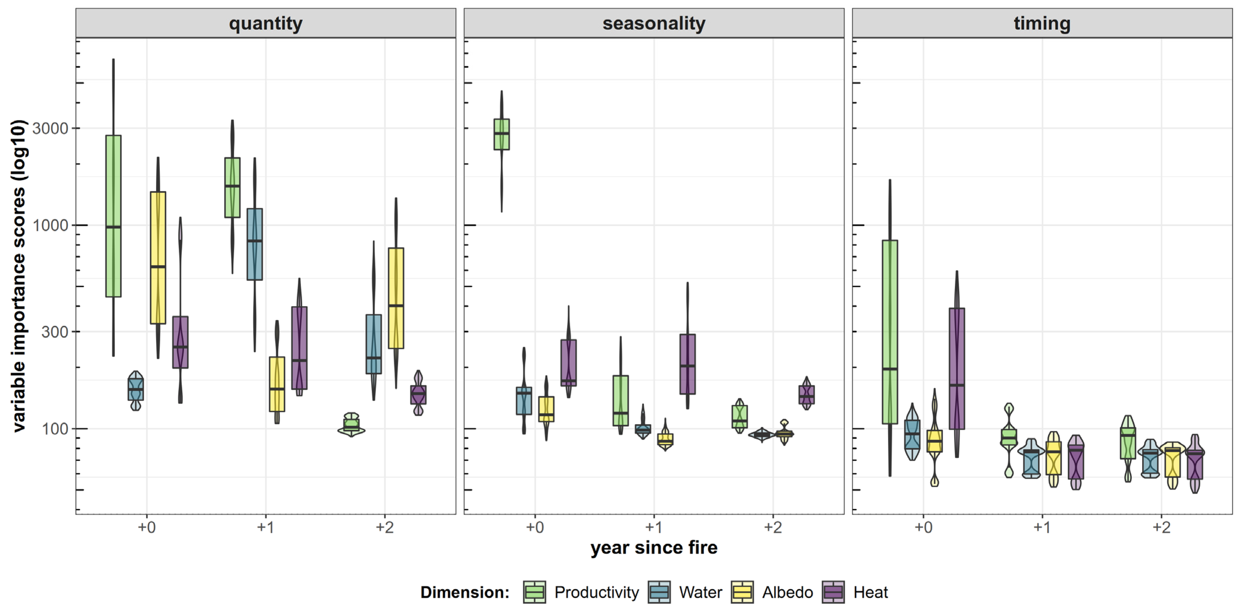
3.1. EFA Ranking
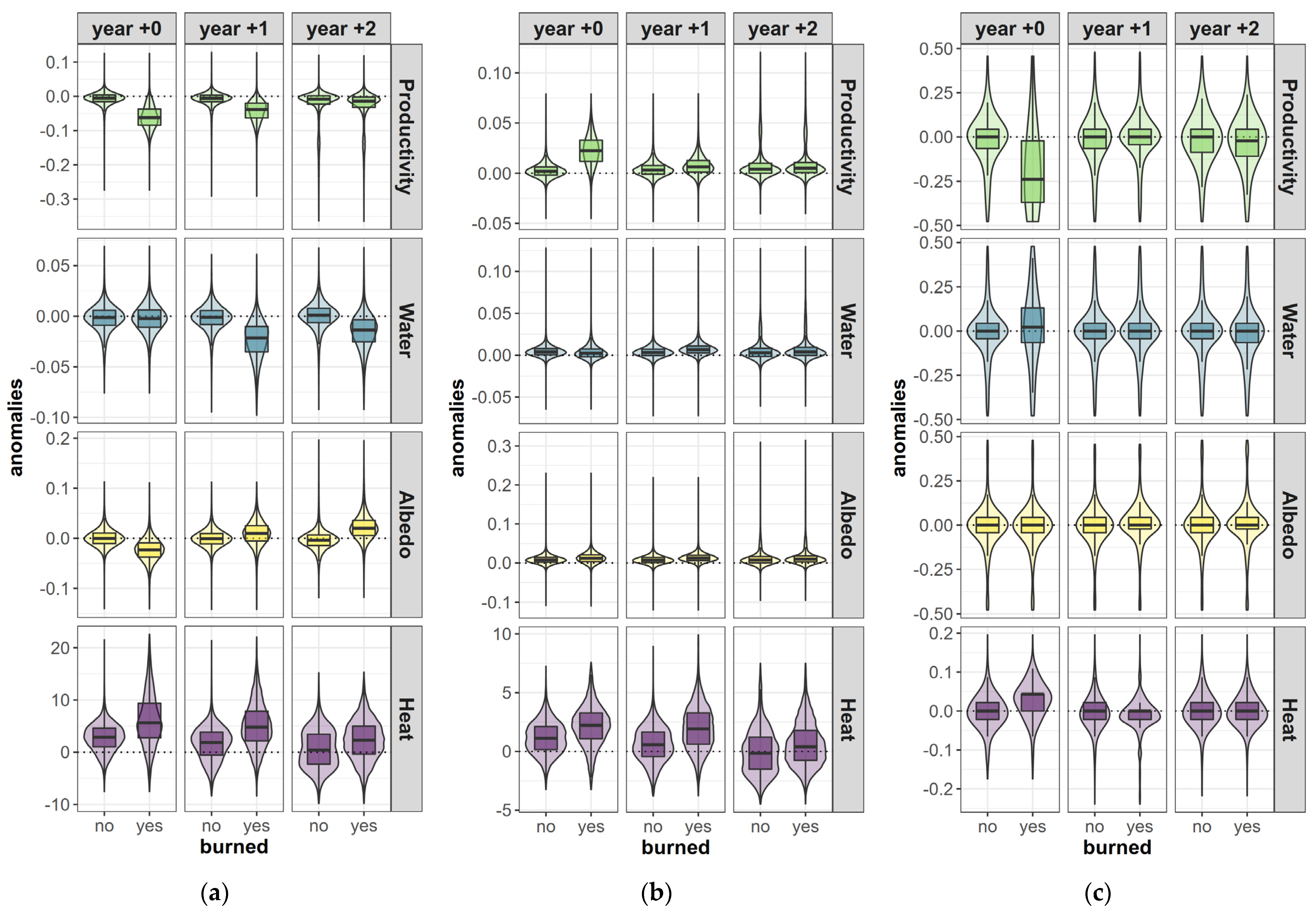
3.2. Analysis of Effects
3.3. Main Patterns in EFA Anomalies
3.4. Multi-Dimensional Assessment of Wildfire Disturbance Severity
4. Discussion
4.1. Fire Severity Patterns in the NW Iberian Peninsula
4.1.1. Effects of Wildfires across Dimensions and Components
4.1.2. Temporal Effects of Wildfires
4.1.3. General Patterns
4.2. General Considerations about the Proposed Framework
4.2.1. Satellite Image Time-Series
4.2.2. Additional Data Sources
4.2.3. Applicability and Future Directions
5. Conclusions
Supplementary Materials
Author Contributions
Funding
Acknowledgments
Conflicts of Interest
References
- Adámek, M.; Hadincová, V.; Wild, J. Long-term effect of wildfires on temperate Pinus sylvestris forests: Vegetation dynamics and ecosystem resilience. For. Ecol. Manag. 2016, 380, 285–295. [Google Scholar] [CrossRef]
- San-Miguel-Ayanz, J.; Moreno, J.M.; Camia, A. Analysis of large fires in European Mediterranean landscapes: Lessons learned and perspectives. For. Ecol. Manag. 2013, 294, 11–22. [Google Scholar] [CrossRef]
- João, T.; João, G.; Bruno, M.; João, H. Indicator-based assessment of post-fire recovery dynamics using satellite NDVI time-series. Ecol. Indic. 2018, 89, 199–212. [Google Scholar] [CrossRef]
- Petropoulos, G.; Carlson, T.; Wooster, M.; Islam, S. A review of Ts/VI remote sensing based methods for the retrieval of land surface energy fluxes and soil surface moisture. Prog. Phys. Georg. Earth Environ. 2009, 33, 224–250. [Google Scholar] [CrossRef] [Green Version]
- Alcaraz-Segura, D.; Cabello, J.; Paruelo, J.M.; Delibes, M. Trends in the surface vegetation dynamics of the national parks of Spain as observed by satellite sensors. Appl. Veg. Sci. 2008, 11, 431–440. [Google Scholar] [CrossRef]
- Wei, X.; Hayes, D.J.; Fraver, S.; Chen, G. Global Pyrogenic Carbon Production During Recent Decades Has Created the Potential for a Large, Long-Term Sink of Atmospheric CO 2. J. Geophys. Res. Biogeosci. 2018, 123, 3682–3696. [Google Scholar] [CrossRef]
- Dunnette, P.V.; Higuera, P.E.; Mclauchlan, K.K.; Derr, K.M.; Briles, C.E.; Keefe, M.H. Biogeochemical impacts of wildfires over four millennia in a Rocky Mountain subalpine watershed. New Phytol. 2014, 203, 900–912. [Google Scholar] [CrossRef]
- Sparks, A.M.; Kolden, C.A.; Smith, A.M.S.; Boschetti, L.; Johnson, D.M.; Cochrane, M.A. Fire intensity impacts on post-fire temperate coniferous forest net primary productivity. Biogeosciences 2018, 15, 1173–1183. [Google Scholar] [CrossRef] [Green Version]
- Pellegrini, A.F.A.; Ahlström, A.; Hobbie, S.E.; Reich, P.B.; Nieradzik, L.P.; Staver, A.C.; Scharenbroch, B.C.; Jumpponen, A.; Anderegg, W.R.L.; Randerson, J.T.; et al. Fire frequency drives decadal changes in soil carbon and nitrogen and ecosystem productivity. Nat. Cell Biol. 2018, 553, 194–198. [Google Scholar] [CrossRef]
- Leys, B.; Higuera, P.; Mclauchlan, K.K.; Dunnette, P.V. Wildfires and geochemical change in a subalpine forest over the past six millennia. Environ. Res. Lett. 2016, 11, 125003. [Google Scholar] [CrossRef]
- Wang, J.; Zhang, X. Impacts of wildfires on interannual trends in land surface phenology: An investigation of the Hayman Fire. Environ. Res. Lett. 2017, 12, 054008. [Google Scholar] [CrossRef]
- Carvalho-Santos, C.; Marcos, B.; Nunes, J.P.; Regos, A.; Palazzi, E.; Terzago, S.; Monteiro, A.T.; Honrado, J.P. Hydrological Impacts of Large Fires and Future Climate: Modeling Approach Supported by Satellite Data. Remote Sens. 2019, 11, 2832. [Google Scholar] [CrossRef] [Green Version]
- Santos, R.; Fernandes, L.S.; Pereira, M.; Cortes, R.; Pacheco, F. Water resources planning for a river basin with recurrent wildfires. Sci. Total Environ. 2015, 526, 1–13. [Google Scholar] [CrossRef] [PubMed]
- Smith, H.G.; Sheridan, G.J.; Lane, P.N.; Nyman, P.; Haydon, S. Wildfire effects on water quality in forest catchments: A review with implications for water supply. J. Hydrol. 2011, 396, 170–192. [Google Scholar] [CrossRef]
- Senf, C.; Seidl, R. Mapping the forest disturbance regimes of Europe. Nat. Sustain. 2021, 4, 63–70. [Google Scholar] [CrossRef]
- Poon, P.K.; Kinoshita, A.M. Spatial and temporal evapotranspiration trends after wildfire in semi-arid landscapes. J. Hydrol. 2018, 559, 71–83. [Google Scholar] [CrossRef]
- Vlassova, L.; Perez-Cabello, F.; Mimbrero, M.R.; Llovería, R.M.; Garcia-Martin, A. Analysis of the Relationship between Land Surface Temperature and Wildfire Severity in a Series of Landsat Images. Remote Sens. 2014, 6, 6136–6162. [Google Scholar] [CrossRef] [Green Version]
- Sun, X.; Zou, C.B.; Wilcox, B.; Stebler, E. Effect of Vegetation on the Energy Balance and Evapotranspiration in Tallgrass Prairie: A Paired Study Using the Eddy-Covariance Method. Bound. Layer Meteorol. 2018, 170, 127–160. [Google Scholar] [CrossRef]
- Liu, Z.; Ballantyne, A.P.; Cooper, L.A. Biophysical feedback of global forest fires on surface temperature. Nat. Commun. 2019, 10, 1–9. [Google Scholar] [CrossRef] [Green Version]
- Rother, D.; De Sales, F. Impact of Wildfire on the Surface Energy Balance in Six California Case Studies. Bound. Layer Meteorol. 2021, 178, 143–166. [Google Scholar] [CrossRef]
- French, N.H.F.; Whitley, M.A.; Jenkins, L.K. Fire disturbance effects on land surface albedo in Alaskan tundra. J. Geophys. Res. Biogeosci. 2016, 121, 841–854. [Google Scholar] [CrossRef] [Green Version]
- Quintano, C.; Fernandez-Manso, A.; Marcos, E.; Calvo, L. Burn Severity and Post-Fire Land Surface Albedo Relationship in Mediterranean Forest Ecosystems. Remote Sens. 2019, 11, 2309. [Google Scholar] [CrossRef] [Green Version]
- Gatebe, C.K.; Ichoku, C.M.; Poudyal, R.; Román, M.; Wilcox, E. Surface albedo darkening from wildfires in northern sub-Saharan Africa. Environ. Res. Lett. 2014, 9, 065003. [Google Scholar] [CrossRef] [Green Version]
- Saha, M.V.; D’Odorico, P.; Scanlon, T.M. Albedo changes after fire as an explanation of fire-induced rainfall suppression. Geophys. Res. Lett. 2017, 44, 3916–3923. [Google Scholar] [CrossRef] [Green Version]
- Liu, H.; Zhan, Q.; Yang, C.; Wang, J. Characterizing the Spatio-Temporal Pattern of Land Surface Temperature through Time Series Clustering: Based on the Latent Pattern and Morphology. Remote Sens. 2018, 10, 654. [Google Scholar] [CrossRef] [Green Version]
- Maffei, C.; Alfieri, S.M.; Menenti, M. Relating Spatiotemporal Patterns of Forest Fires Burned Area and Duration to Diurnal Land Surface Temperature Anomalies. Remote Sens. 2018, 10, 1777. [Google Scholar] [CrossRef] [Green Version]
- Veraverbeke, S.; Verstraeten, W.W.; Lhermitte, S.; Van De Kerchove, R.; Goossens, R. Assessment of post-fire changes in land surface temperature and surface albedo, and their relation with fire—burn severity using multitemporal MODIS imagery. Int. J. Wildland Fire 2012, 21, 243–256. [Google Scholar] [CrossRef] [Green Version]
- Koutsias, N.; Allgöwer, B.; Kalabokidis, K.; Mallinis, G.; Balatsos, P.; Goldammer, J.G. Fire occurrence zoning from local to global scale in the European Mediterranean basin: Implications for multi-scale fire management and policy. iForest Biogeosci. For. 2015, 9, 195–204. [Google Scholar] [CrossRef] [Green Version]
- Bowman, D.M.J.S.; Balch, J.K.; Artaxo, P.; Bond, W.J.; Carlson, J.M.; Cochrane, M.A.; D’Antonio, C.M.; DeFries, R.S.; Doyle, J.C.; Harrison, S.P.; et al. Fire in the Earth System. Science 2009, 324, 481–484. [Google Scholar] [CrossRef] [PubMed]
- Tedim, F.; Remelgado, R.; Borges, C.; Carvalho, S.; Martins, J. Exploring the occurrence of mega-fires in Portugal. For. Ecol. Manag. 2013, 294, 86–96. [Google Scholar] [CrossRef]
- Van Leeuwen, W.J.D.; Casady, G.M.; Neary, D.G.; Bautista, S.; Alloza, J.A.; Carmel, Y.; Wittenberg, L.; Malkinson, D.; Orr, B.J. Monitoring post-wildfire vegetation response with remotely sensed time-series data in Spain, USA and Israel. Int. J. Wildland Fire 2010, 19, 75–93. [Google Scholar] [CrossRef]
- Verbesselt, J.; Hyndman, R.; Zeileis, A.; Culvenor, D. Phenological change detection while accounting for abrupt and gradual trends in satellite image time series. Remote Sens. Environ. 2010, 114, 2970–2980. [Google Scholar] [CrossRef] [Green Version]
- Veraverbeke, S.; Lhermitte, S.; Verstraeten, W.; Goossens, R. A time-integrated MODIS burn severity assessment using the multi-temporal differenced normalized burn ratio (dNBRMT). Int. J. Appl. Earth Obs. Geoinf. 2011, 13, 52–58. [Google Scholar] [CrossRef] [Green Version]
- Bastos, A.; Gouveia, C.M.; Dacamara, C.C.; Trigo, R.M. Modelling post-fire vegetation recovery in Portugal. Biogeosciences 2011, 8, 3593–3607. [Google Scholar] [CrossRef] [Green Version]
- Alcaraz-Segura, D.; Chuvieco, E.; Epstein, H.E.; Kasischke, E.S.; Trishchenko, A. Debating the greening vs. browning of the North American boreal forest: Differences between satellite datasets. Glob. Chang. Biol. 2010, 16, 760–770. [Google Scholar] [CrossRef]
- Frazier, A.E.; Renschler, C.S.; Miles, S.B. Evaluating post-disaster ecosystem resilience using MODIS GPP data. Int. J. Appl. Earth Obs. Geoinf. 2013, 21, 43–52. [Google Scholar] [CrossRef]
- Keeley, J.E. Fire intensity, fire severity and burn severity: A brief review and suggested usage. Int. J. Wildland Fire 2009, 18, 116–126. [Google Scholar] [CrossRef]
- Smith, A.M.; Kolden, C.A.; Tinkham, W.T.; Talhelm, A.F.; Marshall, J.D.; Hudak, A.T.; Boschetti, L.; Falkowski, M.J.; Greenberg, J.A.; Anderson, J.W.; et al. Remote sensing the vulnerability of vegetation in natural terrestrial ecosystems. Remote Sens. Environ. 2014, 154, 322–337. [Google Scholar] [CrossRef]
- Parks, S.A.; Holsinger, L.M.; Koontz, M.J.; Collins, L.; Whitman, E.; Parisien, M.-A.; Loehman, R.A.; Barnes, J.L.; Bourdon, J.-F.; Boucher, Y.; et al. Giving Ecological Meaning to Satellite-Derived Fire Severity Metrics across North American Forests. Remote Sens. 2019, 11, 1735. [Google Scholar] [CrossRef] [Green Version]
- Cardil, A.; Mola-Yudego, B.; Blázquez-Casado, Á.; González-Olabarria, J.R. Fire and burn severity assessment: Calibration of Relative Differenced Normalized Burn Ratio (RdNBR) with field data. J. Environ. Manag. 2019, 235, 342–349. [Google Scholar] [CrossRef]
- Veraverbeke, S.; Lhermitte, S.; Verstraeten, W.; Goossens, R. Evaluation of pre/post-fire differenced spectral indices for assessing burn severity in a Mediterranean environment with Landsat Thematic Mapper. Int. J. Remote Sens. 2011, 32, 3521–3537. [Google Scholar] [CrossRef] [Green Version]
- Bowman, D.M.; Perry, G.L.; Marston, J. Feedbacks and landscape-level vegetation dynamics. Trends Ecol. Evol. 2015, 30, 255–260. [Google Scholar] [CrossRef] [PubMed]
- Quintano, C.; Fernández-Manso, A.; Calvo, L.; Marcos, E.; Valbuena, L. Land surface temperature as potential indicator of burn severity in forest Mediterranean ecosystems. Int. J. Appl. Earth Obs. Geoinf. 2015, 36, 1–12. [Google Scholar] [CrossRef]
- Marcos, B.; Gonçalves, J.; Alcaraz-Segura, D.; Cunha, M.; Honrado, J.P. Improving the detection of wildfire disturbances in space and time based on indicators extracted from MODIS data: A case study in northern Portugal. Int. J. Appl. Earth Obs. Geoinf. 2019, 78, 77–85. [Google Scholar] [CrossRef]
- Coops, N.C.; Wulder, M.A.; Duro, D.C.; Han, T.; Berry, S. The development of a Canadian dynamic habitat index using multi-temporal satellite estimates of canopy light absorbance. Ecol. Indic. 2008, 8, 754–766. [Google Scholar] [CrossRef]
- Alcaraz, D.; Paruelo, J.; Cabello, J. Identification of current ecosystem functional types in the Iberian Peninsula. Glob. Ecol. Biogeogr. 2006, 15, 200–212. [Google Scholar] [CrossRef]
- Duro, D.C.; Coops, N.C.; Wulder, M.A.; Han, T. Development of a large area biodiversity monitoring system driven by remote sensing. Prog. Phys. Geogr. Earth Environ. 2007, 31, 235–260. [Google Scholar] [CrossRef]
- Arenas-Castro, S.; Gonçalves, J.; Alves, P.; Alcaraz-Segura, D.; Honrado, J.P. Assessing the multi-scale predictive ability of ecosystem functional attributes for species distribution modelling. PLoS ONE 2018, 13, e0199292. [Google Scholar] [CrossRef] [Green Version]
- Gonçalves, J.; Alves, P.; Pôças, I.; Marcos, B.; Sousa-Silva, R.; Lomba, Â.; Honrado, J.P. Exploring the spatiotemporal dynamics of habitat suitability to improve conservation management of a vulnerable plant species. Biodivers. Conserv. 2016, 25, 2867–2888. [Google Scholar] [CrossRef]
- Regos, A.; Gómez-Rodríguez, P.; Arenas-Castro, S.; Tapia, L.; Vidal, M.; Domínguez, J. Model-Assisted Bird Monitoring Based on Remotely Sensed Ecosystem Functioning and Atlas Data. Remote Sens. 2020, 12, 2549. [Google Scholar] [CrossRef]
- Cazorla, B.P.; Cabello, J.; Peñas, J.; Garcillán, P.P.; Reyes, A.; Alcaraz-Segura, D. Incorporating Ecosystem Functional Diversity into Geographic Conservation Priorities Using Remotely Sensed Ecosystem Functional Types. Ecosystems 2020, 1–17. [Google Scholar] [CrossRef]
- Paruelo, J.M.; Piñeiro, G.; Escribano, P.; Oyonarte, C.; Alcaraz, D.; Cabello, J. Temporal and spatial patterns of ecosystem functioning in protected arid areas in southeastern Spain. Appl. Veg. Sci. 2005, 8, 93–102. [Google Scholar] [CrossRef]
- Cazorla, B.; Cabello, J.; Reyes, A.; Guirado, E.; Peñas, J.; Pérez-Luque, A.J.; Alcaraz-Segura, D. A remote sensing-based dataset to characterize the ecosystem functioning and functional diversity of a Biosphere Reserve: Sierra Nevada (SE Spain). Earth Syst. Sci. Data Discuss. 2020, 2020, 1–20. [Google Scholar] [CrossRef] [Green Version]
- Arenas-Castro, S.; Regos, A.; Gonçalves, J.F.; Alcaraz-Segura, D.; Honrado, J. Remotely Sensed Variables of Ecosystem Functioning Support Robust Predictions of Abundance Patterns for Rare Species. Remote Sens. 2019, 11, 2086. [Google Scholar] [CrossRef] [Green Version]
- Mildrexler, D.J.; Zhao, M.; Running, S.W. Testing a MODIS Global Disturbance Index across North America. Remote Sens. Environ. 2009, 113, 2103–2117. [Google Scholar] [CrossRef]
- Verbesselt, J.; Hyndman, R.; Newnham, G.; Culvenor, D. Detecting trend and seasonal changes in satellite image time series. Remote Sens. Environ. 2010, 114, 106–115. [Google Scholar] [CrossRef]
- Healey, S.; Cohen, W.; Zhiqiang, Y.; Krankina, O. Comparison of Tasseled Cap-based Landsat data structures for use in forest disturbance detection. Remote Sens. Environ. 2005, 97, 301–310. [Google Scholar] [CrossRef]
- Duan, S.-B.; Li, Z.-L.; Li, H.; Göttsche, F.-M.; Wu, H.; Zhao, W.; Leng, P.; Zhang, X.; Coll, C. Validation of Collection 6 MODIS land surface temperature product using in situ measurements. Remote Sens. Environ. 2019, 225, 16–29. [Google Scholar] [CrossRef] [Green Version]
- Lobser, S.E.; Cohen, W.B. MODIS tasselled cap: Land cover characteristics expressed through transformed MODIS data. Int. J. Remote Sens. 2007, 28, 5079–5101. [Google Scholar] [CrossRef]
- Gouveia, C.A.M.; Dacamara, C.C.; Trigo, R.M. Post-fire vegetation recovery in Portugal based on spot/vegetation data. Nat. Hazards Earth Syst. Sci. 2010, 10, 673–684. [Google Scholar] [CrossRef] [Green Version]
- Cohen, J. A power primer. Psychol. Bull. 1992, 112, 155–159. [Google Scholar] [CrossRef]
- Caon, L.; Vallejo, V.R.; Ritsema, C.J.; Geissen, V. Effects of wildfire on soil nutrients in Mediterranean ecosystems. Earth Sci. Rev. 2014, 139, 47–58. [Google Scholar] [CrossRef]
- Catry, F.X.; Rego, F.C.; Bação, F.L.; Moreira, F. Modeling and mapping wildfire ignition risk in Portugal. Int. J. Wildland Fire 2009, 18, 921–931. [Google Scholar] [CrossRef] [Green Version]
- Yamazaki, D.; Ikeshima, D.; Tawatari, R.; Yamaguchi, T.; O’Loughlin, F.; Neal, J.C.; Sampson, C.C.; Kanae, S.; Bates, P.B. A high-accuracy map of global terrain elevations. Geophys. Res. Lett. 2017, 44, 5844–5853. [Google Scholar] [CrossRef] [Green Version]
- Karger, D.N.; Conrad, O.; Böhner, J.; Kawohl, T.; Kreft, H.; Soria-Auza, R.W.; Zimmermann, N.E.; Linder, H.P.; Kessler, M. Climatologies at high resolution for the earth’s land surface areas. Sci. Data 2017, 4, 170122. [Google Scholar] [CrossRef] [Green Version]
- European Environment Agency (EEA). CLC 2000—Copernicus Land Monitoring Service. Available online: https://land.copernicus.eu/pan-european/corine-land-cover/clc-2000 (accessed on 11 February 2021).
- R Development Core Team R. A Language and Environment for Statistical Computing v 3.5.1; R Foundation for Statistical Computing: Vienna, Austria, 2018; Volume 2, Available online: https://www.R-project.org (accessed on 2 July 2018).
- Hijmans, R.J. Raster: Geographic Data Analysis and Modeling, R Package Version 2.5–8; R Foundation for Statistical Computing: Vienna, Austria, 2016; Available online: https://cran.microsoft.com/snapshot/2016-08-05/web/packages/raster/index.html (accessed on 2 July 2018).
- Busetto, L.; Ranghetti, L. MODIStsp: An R package for automatic preprocessing of MODIS Land Products time series. Comput. Geosci. 2016, 97, 40–48. [Google Scholar] [CrossRef] [Green Version]
- Giglio, L.; Boschetti, L.; Roy, D.P.; Humber, M.L.; Justice, C.O. The Collection 6 MODIS burned area mapping algorithm and product. Remote Sens. Environ. 2018, 217, 72–85. [Google Scholar] [CrossRef] [PubMed]
- Wan, Z.; Hook, S.; Hulley, G. MOD11A2 MODIS/Terra Land Surface Temperature/Emissivity 8-Day L3 Global 1km SIN Grid V006. NASA EOSDIS Land Process. DAAC 2015, 10. Available online: https://lpdaac.usgs.gov/products/mod11a2v006/ (accessed on 19 February 2021).
- Vermote, E. MOD09A1 MODIS/Terra Surface Reflectance 8-Day L3 Global 500m SIN Grid V006. NASA EOSDIS Land Process. DAAC 2015, 10. Available online: https://lpdaac.usgs.gov/products/mod09a1v006/ (accessed on 19 February 2021).
- Hampel, F.R. A General Qualitative Definition of Robustness. Ann. Math. Stat. 1971, 42, 1887–1896. [Google Scholar] [CrossRef]
- Hampel, F.R. The Influence Curve and its Role in Robust Estimation. J. Am. Stat. Assoc. 1974, 69, 383–393. [Google Scholar] [CrossRef]
- GDAL. Geospatial Data Abstraction Library v 3.0.4. 2020. Available online: https://gdal.org/ (accessed on 28 January 2020).
- Gillies, S.; Ward, B.; Petersen, A.S. Rasterio: Geospatial Raster I/O for Python Programmers. 2013. Available online: https//github.com/mapbox/rasterio (accessed on 15 July 2018).
- Whittaker, E.T. On a New Method of Graduation. Proc. Edinb. Math. Soc. 1922, 41, 63–75. [Google Scholar] [CrossRef] [Green Version]
- Eilers, P.H.C. A Perfect Smoother. Anal. Chem. 2003, 75, 3631–3636. [Google Scholar] [CrossRef]
- Couronné, R.; Probst, P.; Boulesteix, A.-L. Random forest versus logistic regression: A large-scale benchmark experiment. BMC Bioinform. 2018, 19, 1–14. [Google Scholar] [CrossRef] [PubMed]
- Kuhn, M.; Weston, S.; Keefer, C.; Engelhardt, A.; Cooper, T.; Mayer, Z.; Kenkel, B.; Team, R.C.; Benesty, M.; Lescarbeau, R.; et al. Caret: Classification and Regression Training, R Package v 6.0–70; R Foundation for Statistical Computing: Vienna, Austria, 2016; Available online: https://CRAN.R-project.org/package=caret (accessed on 2 July 2018).
- Wasserstein, R.L.; Lazar, N.A. The ASA Statement on p-Values: Context, Process, and Purpose. Am. Stat. 2016, 70, 129–133. [Google Scholar] [CrossRef] [Green Version]
- Hubbard, R.; Lindsay, R.M. Why P Values Are Not a Useful Measure of Evidence in Statistical Significance Testing. Theory Psychol. 2008, 18, 69–88. [Google Scholar] [CrossRef]
- Mack, M.C.; Bret-Harte, M.S.; Hollingsworth, T.N.; Jandt, R.R.; Schuur, E.A.G.; Shaver, G.R.; Verbyla, D.L. Carbon loss from an unprecedented Arctic tundra wildfire. Nat. Cell Biol. 2011, 475, 489–492. [Google Scholar] [CrossRef] [PubMed]
- Ramanathan, V.; Carmichael, G. Global and regional climate changes due to black carbon. Nat. Geosci. 2008, 1, 221–227. [Google Scholar] [CrossRef]
- Volante, J.; Alcaraz-Segura, D.; Mosciaro, M.; Viglizzo, E.; Paruelo, J. Ecosystem functional changes associated with land clearing in NW Argentina. Agric. Ecosyst. Environ. 2012, 154, 12–22. [Google Scholar] [CrossRef]
- Bodí, M.B.; Martin, D.A.; Balfour, V.N.; Santín, C.; Doerr, S.H.; Pereira, P.R.G.; Cerdà, A.; Mataix-Solera, J. Wildland fire ash: Production, composition and eco-hydro-geomorphic effects. Earth Sci. Rev. 2014, 130, 103–127. [Google Scholar] [CrossRef]
- Saha, M.V.; D’Odorico, P.; Scanlon, T.M. Kalahari Wildfires Drive Continental Post-Fire Brightening in Sub-Saharan Africa. Remote Sens. 2019, 11, 1090. [Google Scholar] [CrossRef] [Green Version]
- Lentile, L.B.; Holden, Z.A.; Smith, A.M.S.; Falkowski, M.J.; Hudak, A.T.; Morgan, P.; Lewis, S.A.; Gessler, P.E.; Benson, N.C. Remote sensing techniques to assess active fire characteristics and post-fire effects. Int. J. Wildland Fire 2006, 15, 319–345. [Google Scholar] [CrossRef]
- García-Llamas, P.; Suárez-Seoane, S.; Taboada, A.; Fernández-Manso, A.; Quintano, C.; Fernández-García, V.; Fernández-Guisuraga, J.M.; Marcos, E.; Calvo, L. Environmental drivers of fire severity in extreme fire events that affect Mediterranean pine forest ecosystems. For. Ecol. Manag. 2019, 433, 24–32. [Google Scholar] [CrossRef]
- Mallinis, G.; Mitsopoulos, I.; Chrysafi, I. Evaluating and comparing Sentinel 2A and Landsat-8 Operational Land Imager (OLI) spectral indices for estimating fire severity in a Mediterranean pine ecosystem of Greece. Geosci. Remote Sens. 2017, 55, 1–18. [Google Scholar] [CrossRef]
- Shi, T.; Xu, H. Derivation of Tasseled Cap Transformation Coefficients for Sentinel-2 MSI At-Sensor Reflectance Data. IEEE J. Sel. Top. Appl. Earth Obs. Remote Sens. 2019, 12, 4038–4048. [Google Scholar] [CrossRef]
- Marcos, E.; Fernández-García, V.; Fernández-Manso, A.; Quintano, C.; Valbuena, L.; Tárrega, R.; Luis-Calabuig, E.; Calvo, L. Evaluation of Composite Burn Index and Land Surface Temperature for Assessing Soil Burn Severity in Mediterranean Fire-Prone Pine Ecosystems. Forests 2018, 9, 494. [Google Scholar] [CrossRef] [Green Version]
- De Santis, A.; Chuvieco, E. GeoCBI: A modified version of the Composite Burn Index for the initial assessment of the short-term burn severity from remotely sensed data. Remote Sens. Environ. 2009, 113, 554–562. [Google Scholar] [CrossRef]
- Landi, M.A.; Bella, C.M.D.; Bravo, S.J.; Bellis, L.M. Structural resistance and functional resilience of the Chaco forest to wildland fires: An approach with MODIS time series. Aust. Ecol. 2020. [Google Scholar] [CrossRef]
- Fernández, N.; Paruelo, J.M.; Delibes, M. Ecosystem functioning of protected and altered Mediterranean environments: A remote sensing classification in Doñana, Spain. Remote Sens. Environ. 2010, 114, 211–220. [Google Scholar] [CrossRef]
- Cocking, M.I.; Varner, J.M.; Knapp, E.E. Long-term effects of fire severity on oak-conifer dynamics in the southern Cascades. Ecol. Appl. 2014, 24, 94–107. [Google Scholar] [CrossRef]


| NW-IP | A | B | C | D | |
|---|---|---|---|---|---|
| Year of fire | ― | 2003 | 2005 | 2005 | 2013 |
| Average burned area (ha) | 3617 | 14,625 | 17,600 | 19,325 | 14,850 |
| Distance to coast (km) | ― | 212 | 9 | 91 | 153 |
| Average elevation (m a.s.l.) | 580 | 801 | 261 | 712 | 505 |
| Average temperature (°C) | 12.7 | 13.0 | 14.1 | 12.5 | 14.1 |
| Minimum temperature (°C) | 3.1 | 1.2 | 7.5 | 1.0 | 2.8 |
| Maximum temperature (°C) | 2.5 | 28.9 | 21.8 | 26.7 | 29.1 |
| Average total precipitation (mm·yr−1) | 1139 | 1075 | 1747 | 1229 | 620 |
| % of Urban | 1.8 | 0.0 | 1.1 | 0.1 | 0.2 |
| % of Agricultural | 29.0 | 9.3 | 8.0 | 5.8 | 26.0 |
| % of Broad-leaf forests | 7.1 | 0.8 | 1.6 | 0.2 | 4.9 |
| % of Coniferous forests | 5.9 | 34.5 | 17.7 | 32.8 | 10.8 |
| % of Mixed forests | 8.7 | 4.5 | 9.1 | 3.4 | 1.5 |
| % of Natural grasslands | 5.6 | 0.2 | 4.0 | 0.0 | 17.4 |
| % of Shrublands | 20.2 | 50.1 | 32.7 | 57.1 | 38.2 |
| % of Bare rocks or sparsely vegetated | 2.0 | 0.6 | 25.7 | 0.6 | 1.0 |
| Band | Coefficients | ||||
|---|---|---|---|---|---|
| No. | Name | Range (nm) | Brightness | Greenness | Wetness |
| 1 | Red | 620–670 | 0.4395 | –0.4064 | 0.1147 |
| 2 | NIR 1 | 841–876 | 0.5945 | 0.5129 | 0.2489 |
| 3 | Blue | 459–479 | 0.2460 | –0.2744 | 0.2408 |
| 4 | Green | 545–565 | 0.3918 | –0.2893 | 0.3132 |
| 5 | NIR 2 | 1230–1250 | 0.3506 | 0.4882 | –0.3122 |
| 6 | SWIR 1 | 1628–1652 | 0.2136 | –0.0036 | –0.6416 |
| 7 | SWIR 2 | 2105–2155 | 0.2678 | –0.4169 | –0.5087 |
| Component | Metric | Abbreviation | No. of Variables for Models |
|---|---|---|---|
| Quantity | Mean (or average) | avg | 12 |
| Median | mdn | 12 | |
| Maximum | max | 12 | |
| Minimum | min | 12 | |
| Seasonality | Standard deviation | std | 12 |
| Median absolute deviation | mad | 12 | |
| Absolute range | rng | 12 | |
| Relative range | rrl | 12 | |
| Non-parametric relative range | rnp | 12 | |
| Timing | Time (of the year) of maximum | tmx | 12 |
| “Winterness” of maximum | wmx | 12 | |
| “Springness” of maximum | smx | 12 | |
| Time (of the year) of minimum | tmn | 12 | |
| “Winterness” of minimum | wmn | 12 | |
| “Springness” of minimum | smn | 12 | |
| Total | 180 |
| Dimension | Component | Attributes (EFA) | Effect Category | ||
|---|---|---|---|---|---|
| Year 0 | Year +1 | Year +2 | |||
| Primary productivity | Quantity | TCTG-min | ↘↘↘ | ↘↘↘ | ― |
| Seasonality | TCTG-std | ↗↗↗ | ↗↗ | ― | |
| Timing | TCTG-tmn | ↘↘↘ | ― | ― | |
| Vegetation water content | Quantity | TCTW-avg | ↘↘↘ | ↘↘↘ | |
| Seasonality | TCTW-std | ― | ↗↗ | ― | |
| Timing | TCTW-tmn | ― | ― | ― | |
| Albedo | Quantity | TCTB-avg | ↘↘↘ | ↗ | ↗↗↗ |
| Seasonality | TCTB-std | ― | ↗ | ― | |
| Timing | TCTB-tmx | ― | ― | ― | |
| Sensible heat | Quantity | LST-max | ↗↗↗ | ↗↗↗ | ↗ |
| Seasonality | LST-std | ↗↗ | ↗↗↗ | ↗ | |
| Timing | LST-tmx | ↗↗↗ | ― | ― | |
Publisher’s Note: MDPI stays neutral with regard to jurisdictional claims in published maps and institutional affiliations. |
© 2021 by the authors. Licensee MDPI, Basel, Switzerland. This article is an open access article distributed under the terms and conditions of the Creative Commons Attribution (CC BY) license (http://creativecommons.org/licenses/by/4.0/).
Share and Cite
Marcos, B.; Gonçalves, J.; Alcaraz-Segura, D.; Cunha, M.; Honrado, J.P. A Framework for Multi-Dimensional Assessment of Wildfire Disturbance Severity from Remotely Sensed Ecosystem Functioning Attributes. Remote Sens. 2021, 13, 780. https://0-doi-org.brum.beds.ac.uk/10.3390/rs13040780
Marcos B, Gonçalves J, Alcaraz-Segura D, Cunha M, Honrado JP. A Framework for Multi-Dimensional Assessment of Wildfire Disturbance Severity from Remotely Sensed Ecosystem Functioning Attributes. Remote Sensing. 2021; 13(4):780. https://0-doi-org.brum.beds.ac.uk/10.3390/rs13040780
Chicago/Turabian StyleMarcos, Bruno, João Gonçalves, Domingo Alcaraz-Segura, Mário Cunha, and João P. Honrado. 2021. "A Framework for Multi-Dimensional Assessment of Wildfire Disturbance Severity from Remotely Sensed Ecosystem Functioning Attributes" Remote Sensing 13, no. 4: 780. https://0-doi-org.brum.beds.ac.uk/10.3390/rs13040780