UAV Based Estimation of Forest Leaf Area Index (LAI) through Oblique Photogrammetry
by
 , ,
, ,
Lingchen Lin
1,2, 
Kunyong Yu
1,2,
Xiong Yao
2,3,
Yangbo Deng
1,2,
Zhenbang Hao
1,2,
Yan Chen
1,2,
Nankun Wu
1,2 and
Jian Liu
1,2,* 1
College of Forestry, Fujian Agriculture and Forestry University, Fuzhou 350002, Fujian, China
2
University Key Lab for Geomatics Technology and Optimize Resources Utilization in Fujian Province, Fuzhou 350002, Fujian, China
3
College of Architecture and Urban Planning, Fujian University of Technology, Fuzhou 350118, Fujian, China
*
Author to whom correspondence should be addressed.
Remote Sens. 2021, 13(4), 803; https://0-doi-org.brum.beds.ac.uk/10.3390/rs13040803
Submission received: 8 January 2021
/
Revised: 12 February 2021
/
Accepted: 18 February 2021
/
Published: 22 February 2021
(This article belongs to the Section Forest Remote Sensing)
Abstract
:As a key canopy structure parameter, the estimation method of the Leaf Area Index (LAI) has always attracted attention. To explore a potential method to estimate forest LAI from 3D point cloud at low cost, we took photos from different angles of the drone and set five schemes (O (0°), T15 (15°), T30 (30°), OT15 (0° and 15°) and OT30 (0° and 30°)), which were used to reconstruct 3D point cloud of forest canopy based on photogrammetry. Subsequently, the LAI values and the leaf area distribution in the vertical direction derived from five schemes were calculated based on the voxelized model. Our results show that the serious lack of leaf area in the middle and lower layers determines that the LAI estimate of O is inaccurate. For oblique photogrammetry, schemes with 30° photos always provided better LAI estimates than schemes with 15° photos (T30 better than T15, OT30 better than OT15), mainly reflected in the lower part of the canopy, which is particularly obvious in low-LAI areas. The overall structure of the single-tilt angle scheme (T15, T30) was relatively complete, but the rough point cloud details could not reflect the actual situation of LAI well. Multi-angle schemes (OT15, OT30) provided excellent leaf area estimation (OT15: R2 = 0.8225, RMSE = 0.3334 m2/m2; OT30: R2 = 0.9119, RMSE = 0.1790 m2/m2). OT30 provided the best LAI estimation accuracy at a sub-voxel size of 0.09 m and the best checkpoint accuracy (OT30: RMSE [H] = 0.2917 m, RMSE [V] = 0.1797 m). The results highlight that coupling oblique photography and nadiral photography can be an effective solution to estimate forest LAI.
1. Introduction
Leaf area index (LAI) is defined as half of the total leaf area per unit ground surface area [1,2,3] and is a critical parameter in many forest process models. As a key canopy structure feature, LAI controls the biophysical processes of the forest (photosynthesis, respiration, transpiration, carbon cycle and precipitation interception, etc.) [4]. Therefore, it is important to estimate LAI quickly and accurately.
Many field-based methods have been developed for LAI distribution estimation, but they are still time-consuming and labor-intensive work, cause permanent damage to the forest [5,6] or are affected by many factors (such as leaf distribution, canopy shape and sampling scale) [7]. Multispectral data from satellite or unmanned aerial vehicle (UAV) have been widely used in the inversion of forest LAI in the past. However, two-dimensional images based on optical passive remote sensing often ignore the leaf area of the middle and lower canopy, which will cause inaccurate estimation of LAI [8,9]. Point clouds data can directly reflect the three-dimensional structure of the canopy, which is widely used in the distribution of forest LAI. However, the point clouds from high-resolution terrestrial LiDAR (TLS) require extensive data collection [10], which is inconvenient to apply on a large scale. Compared with TLS, airborne laser scanning (ALS) point clouds require less labor, but its expensive price is unreasonable in continuous large-scale forest parameter monitoring [11].
Recently, various photogrammetry technologies of generating 3D scenes from 2D images (shape from texture (SFT) [12,13], shape from shading (SFS) [14,15,16], structure-from-motion and multi-view stereo (SFM-MVS) workflow ([17]; etc.) have been developed in the field of computer vision to obtain three-dimensional point clouds of object surfaces at very low cost. Among these methods, the SFM–MVS workflow is the most efficient for reconstructing 3D structure of a scene by analyzing the geometric constraints between the image sequences captured by cameras in different positions [18]. The SFM–MVS workflow has been successfully applied to single-wood level 3D reconstructions based on ground photography [19]. However, large-scale ground surface 3D reconstruction based on drone photography still faces various challenges like positioning accuracy, camera and lens posture correction. Traditional photogrammetry generally only uses drone orthophotos as raw materials for the SFM-MVS workflow [20,21,22] because of the excellent homology point matching results, but which will result in incomplete three-dimensional canopy structures in forest scenes. The point cloud information derived from SFM-MVS is closely related to the content contained in the pixels of the original photo. Due to the canopy occlusion effect, the canopy information obtained by nadir photos is generally missing, mainly in the middle and lower part of the canopy, which will seriously underestimate the leaf area estimation. Recently, oblique photography has attracted great attention as photos from tilt angles and can obtain more side structure of target scenarios than nadiral photography [23,24,25], which overcomes the limitation of traditional photogrammetry. Hence, coupling photos from different lens angles based on the SFM-MVS workflow should result in a relatively complete forest canopy structure.
In this study, we focused on using the photogrammetry (SFM-MVS) to reconstruct forest canopy structure and further estimate the forest LAI. To avoid serious loss of the middle and lower canopy structure, we used unmanned aerial vehicle (UAV) photos taken from different angles as raw materials to reconstruct the point clouds of the Masson pine. We set up five angle combinations (0°, 15°, 30°, 0° and 15°, 0° and 30°) to further explore the impact of different angle-image combinations on the accuracy of forest leaf area estimation. Meanwhile, voxelized models of different sizes were constructed to explore the impact of subvoxel size on LAI estimation accuracy, as the size of sub-voxels is an important factor that affects the accuracy of forest leaf area estimation. By coupling oblique photos and nadir photos from UAV, we propose a potential solution to improve the LAI estimation based on drone point clouds.
2. Materials and Methods
2.1. Overview of Study Region
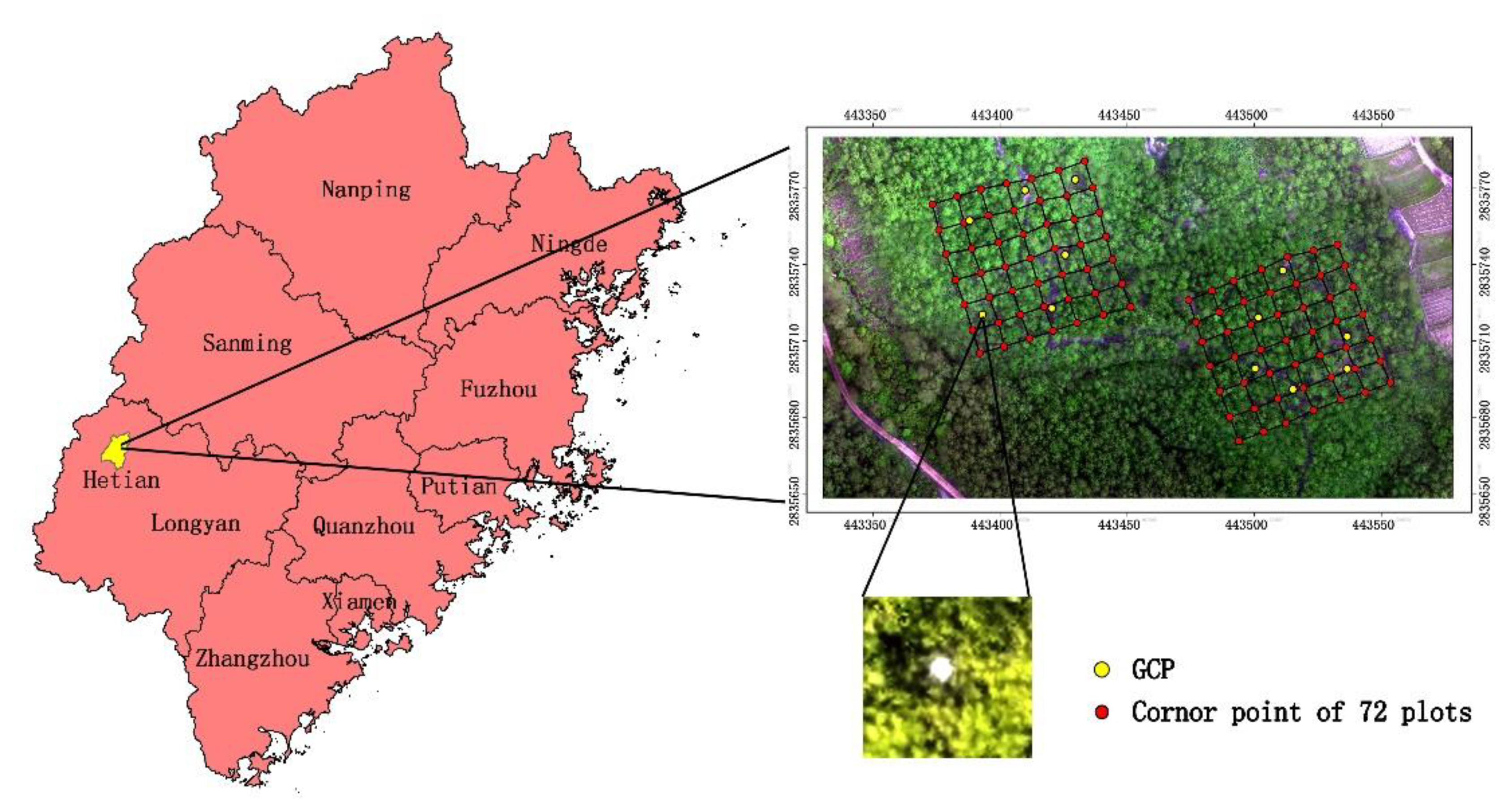
Our research site was approximately 85 acres located in Hetian, Changting County, Fujian Province, China (25°33′–25°48′N, 116°72′–116°31′E). The dominant tree species in this area is the Masson pine (Pinus massoniana), which accounts for about 80% of the study area; other trees included Schima superba, Cyclobalanopsis gracilis and Lespedeza bicolor, which are scarce in the study area. The undergrowth vegetation was dominated by Dicranopteris linearis. Here, we set up 72 sample plots of pure masson pine forests, each 10 × 10 m (Figure 1).
2.2. UAV Parameters and Flight-Scheme Design
DJI Phantom 4 drone equipped with multispectral sensors (Phantom 4, DJ-Innovations, Shenzhen, China) was used to collect aerial images. The DJI Phantom 4 multispectral version is a vertical-lift quadrotor drone with real-time kinematics (RTK). The network RTK produced an average accuracy of 1.5 cm horizontally and 1 cm vertically. The maximum photo resolution was 1600 × 1300 px (4:3.25); the ground sampling distance was (H/18.9) cm/pixel (H is flying height). The effective lens field of vision was 62.7°, and focal length was 5.74 mm. The rotation angle of the PTZ was pitch: −90° to + 30°.
To obtain more detailed forest canopy information, we used a visible light camera on a UAV to take photos in the same route with different lens angles. Considering that an excessively large lens tilt angle would result in a lower homology point-matching relationship, we acquired two oblique image sets (15°, 30°) and one nadir photo set (0°). The overlap rate of the UAV flight course heading and side direction was 85% at a flying height of 120 m. Taking into account the particularity of the view of oblique photography, we used an orthogonal flight to obtain oblique photos (Figure 2), which was implemented in two phases (N–S and E–W). Despite the field of view of the nadir photo being the same in all directions, orthogonal flight plans are also used to obtain nadir photos to ensure that the results are comparable. RTK was used to accurately locate the pre-arranged ground control points (GCP) around the 72 sample plots to determine the coordinate accuracy of the derived point cloud and the point cloud coordinate registration (Figure 1).
2.3. Methods
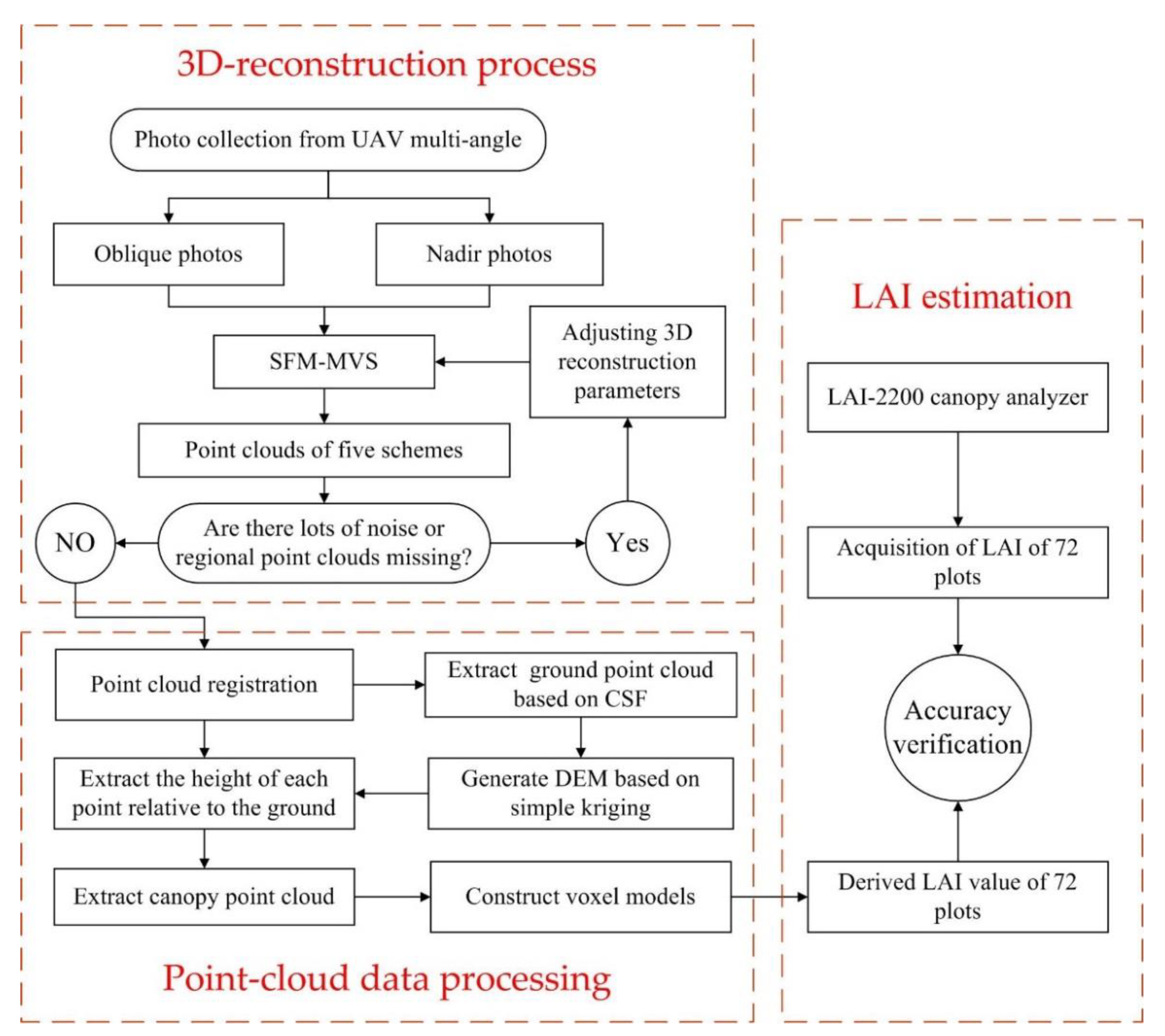
The specific methods followed in this study are summarized in Figure 3, which is mainly divided into three parts: (1) 3D-reconstruction process; (2) point-cloud data processing; (3) LAI estimation. The code for voxelization model and LAI fast extraction is detailed in the attachment.
2.3.1. Three-Dimensional Reconstruction Process
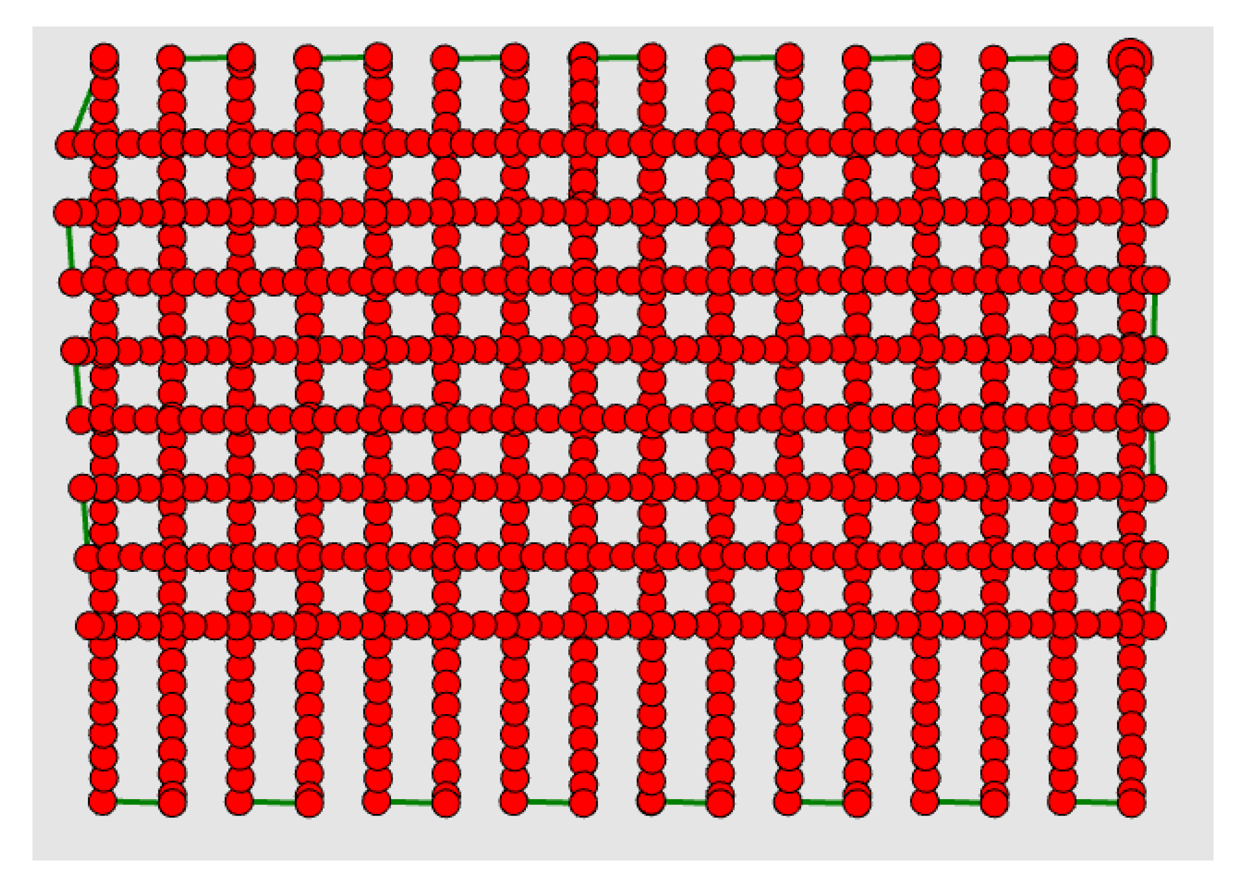
SFM-MVS workflow can couple photos well from different angles to restore 3D structure and consists of two steps: (1) structure-from-motion (SFM) and (2) multi-view stereo (MVS). The SFM algorithm is a motion photogrammetric technique used to reconstruct 3D point clouds from high-overlapping images [26], the derived point clouds of which are sparse. In the second step, multi-view stereo (MVS) reconstructs dense point clouds based on sparse point clouds and image-feature-matching results, camera position, attitude and internal parameters calculated by SFM [27]. To explore the influence of UAV images taken from different angles on the 3D reconstruction of Masson pine forest, we set up five solutions for point-cloud reconstruction through the forms of single angle and multiple angles: (1) O (0°), (2) T15 (15°), (3) T30 (30°), (4) OT15 (0° and 15°) and (5) OT30 (0° and 30°). The images were processed on Pix4 D (version 4.3, Pix4 D, Prilly, Switzerland), which can automatically construct 3D structure based on the SFM-MVS algorithm. The SFM process of Pix4 D starts with image-feature detection. In this critical step, homology-matching points are obtained, which are later used for generating image correspondence. Next, a sparse point cloud is generated based on iterative bundle adjustment (BA) [28]. The image matching result is the decisive factor to decide whether the surface model is complete or not. After using different parameters for image matching, we found that when the number of adjacent images is set to 4 or more and the self-calibration scheme is set to “precise geolocation and direction”, an effective homologous point matching result is derived (Figure 4). Meanwhile, geometric verification matching can provide accurate and effective image matching. In the phase of generating point cloud and encrypting point cloud, we set the density of point cloud and image scale to the highest to ensure the integrity of canopy structure.
2.3.2. Point-Cloud Data Processing
To compare the LAI estimates of different schemes (O, OT15, OT30, T15, T30) with comparability, we used GCP coordinates pre-arranged around the sample site [29] for point-cloud registration, which was performed in CloudCompare (http://cloudcompare.org/ (accessed on 17 July 2020)). Redundant ground point clouds overestimate the final LAI estimation result, so all ground point clouds and noise should be eliminated before constructing the voxel model. Even though the automatic point cloud classification function of the Pix4 d software is very convenient, the classification results often have wrong estimates and cause the separated ground points to be too sparse. Therefore, we chose another method (Cloth Simulation Filter) to extract ground point clusters. Cloth Simulation Filter (CSF) is a tool that can extract ground points by simply setting a few parameters [30,31]. The cloth resolution refers to the size of cloth used to cover the terrain. Excessive cloth resolution will result in rough ground point clouds. The CSF process was executed in Cloudcompare using the following parameters: the general parameter was set to a steep slope, the cloth resolution was 0.5 m, the maximum iteration was 500 and the classification threshold was 0.1 m. Then, we used the simple kriging method in the geostatistical module of ArcGIS (version 10.2, ESRI, Redlands, CA, USA) to interpolate the ground point clouds to obtain the DEM data. Finally, the Z-value of each point coordinate was subtracted from the height value of the corresponding position in the DEM to obtain the height value of the point clouds relative to the ground. The derived point clouds collection also included forest canopy, ground vegetation, soil, etc. Notably, the collection of non-canopy point clouds can lead to the overestimation of leaf area in the lower part of the stand. Therefore, it was necessary to eliminate the non-canopy point-cloud collections. The height of the Masson pine branches in the study area was generally about 2 m, so we used 2 m as a dividing limit to delete the non-canopy point-cloud collection. The elimination of noise was performed in MATLAB software (version 2018 a, MathWorks, Natick, MA, USA) according to the following specific steps: 1. Use KNNSearch to retrieve the 30 nearest points of each point. 2. Calculate the average distance between each point and the 30 nearest neighbors and the mean and standard deviation of these average distances. If the difference between the average distance from a point to the 30 nearest neighbors and the mean is not within 1 times the standard deviation, it is considered a noise point and deleted.
2.3.3. LAI Calculation Method
Point-cloud data derived from UAV images do not reflect details at a single-tree level well. Thus, we followed the method developed by Hosoi and Omasa [32] to construct a voxel model. Using the voxel model to calculate LAI can avoid recalculating the unilateral leaf area of the same leaf. The point-cloud coordinates was converted in MATLAB into voxelized array, which contained both a 0.5 × 0.5 × 0.5 m voxelized model and a sub-voxelized model. To compare the leaf area estimation capabilities of point clouds derived from different schemes at different heights of the canopy, we extracted the leaf area density (LAD) distribution, defined as the sum of the unilateral leaf area per unit volume [33], at different heights of the canopy from the ground from the voxel model. Then, the derived LAI was calculated based on the principle that the integral of LAD in the vertical direction is equal to the LAI. Clearings in the forest that did not contain point clouds could not be retrieved with the voxelized array, which would cause leaf-area overestimation. The sub-voxel size was the most critical factor in determining the estimated value of leaf area. To explore the appropriate sub-voxel size of the derived point clouds for leaf area estimation, we set up ten 0.06 to 0.15 m side-length sub-voxels in steps of 0.01 m, according to the point-cloud density in the report from Pix4 D. For these areas, we added the coordinates of the blank voxels in the voxelized array and set the LAD value of these blank voxels to 0. Then, the forest stands were stratified according to the height, and the forest LAD was calculated using a stratification interval of 0.5 m. We used the average LAD values of all voxels in each 0.5 m layer within each plot range as the LAD value of the layer.
2.3.4. LAI Field Measurement
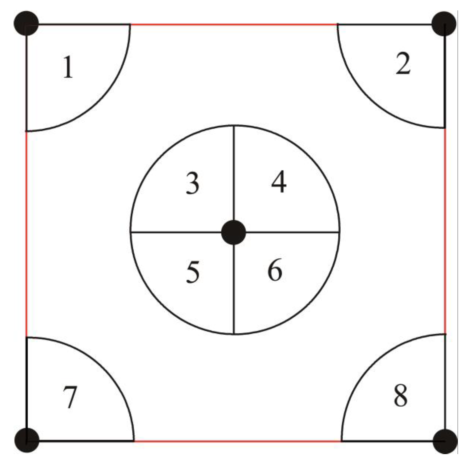
To obtain the optimal sub-voxel size interval for leaf area calculation, we adopted the leaf area index LAI of each plot. The LAI-2200 canopy analyzer—equipped with 90° covering cap—was used to measure the LAI values of 72 plots on a cloudy day without rain. For each sample plot, we took the center and four corners as measurement sites (Figure 5). When measuring at the corner of the sample plot, the probe of LAI-2200 points to the center, and when measuring at the center of the sample plot, the probe of LAI-2200 points to the corner (Figure 5), and finally, the average value of eight measurement results is taken as the LAI value of sample plot. The measurement was repeated three times on each sample plot according to the same method. The outliers were removed, and the average of the remaining data were taken as the final LAI value of each plot.
Although the LAI obtained by the LAI-2200 is actually the effective leaf area index (LAIe), many studies use it to replace LAI because it is difficult to remove the influence of non-leaf components [34]. The LAI values derived from the voxelized models of different sub-voxel sizes and the LAI values measured on-site using the LAI 2200 canopy analyzer were used for linear fitting. Then, the interval of the sub-voxel size most suitable for LAI estimation for each scheme was judged by comparing the slope (a), intercept (b), correlation coefficient (R2) of the fitted linearity and the root mean square error (RMSE) between the two sets of data. Generally speaking, the derived LAI is closer to LAIe when the R2 and slope (a) are closer to 1 and the intercept (b) and RMSE are closer to 0.
3. Results
3.1. Point Clouds Coordinates Accuracy Assessments
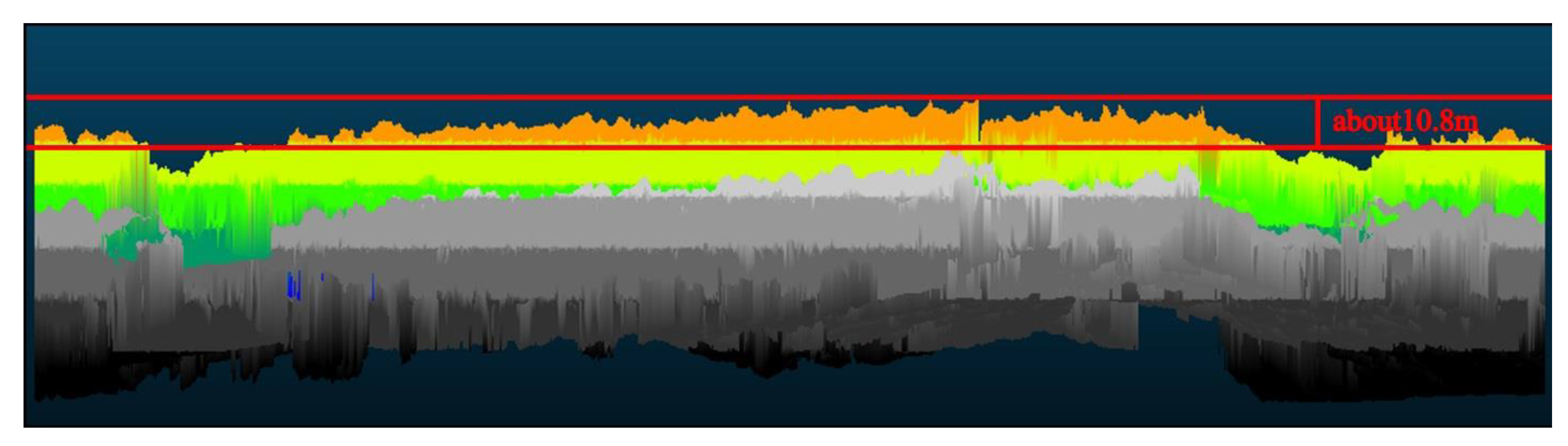
All the point clouds collections of the five schemes were generated from photos combining of different angles without using GCP. The coordinates of GCP collected from derived point clouds were compared with the coordinates collected by RTK (Figure 6). On the premise that GCP coordinates are not incorporated in the bundle adjustment (BA), OT30 gave the lowest horizontal and vertical checkpoint coordinate error. O gave the highest checkpoint coordinate error (O: RMSE [H] = 1.2410 m, RMSE [V] = 10.8862 m), and the vertical error was even more than 10 m (Figure 6(a2)). The checkpoint accuracy of the surface models obtained by coupling the nadir photo and the oblique photo (OT15, OT30) was higher than that of the single-angle schemes (O, T15, T30). The addition of 30° photos improved the coordinate accuracy better than that of 15° photos (OT30: RMSE (H) = 0.2917 m, RMSE (V) = 0.1797 m; OT15: RMSE (H) = 0.4696 m, RMSE (V) = 0.3953 m). After point-clouds registration, the coordinate errors of the five schemes all fluctuate between 0.1 m and 0.14 m (Figure 6(b1,b2)), which is sufficient for a sample plot with a side length of 10 m.
3.2. LAI Retrieval from Five Schemes
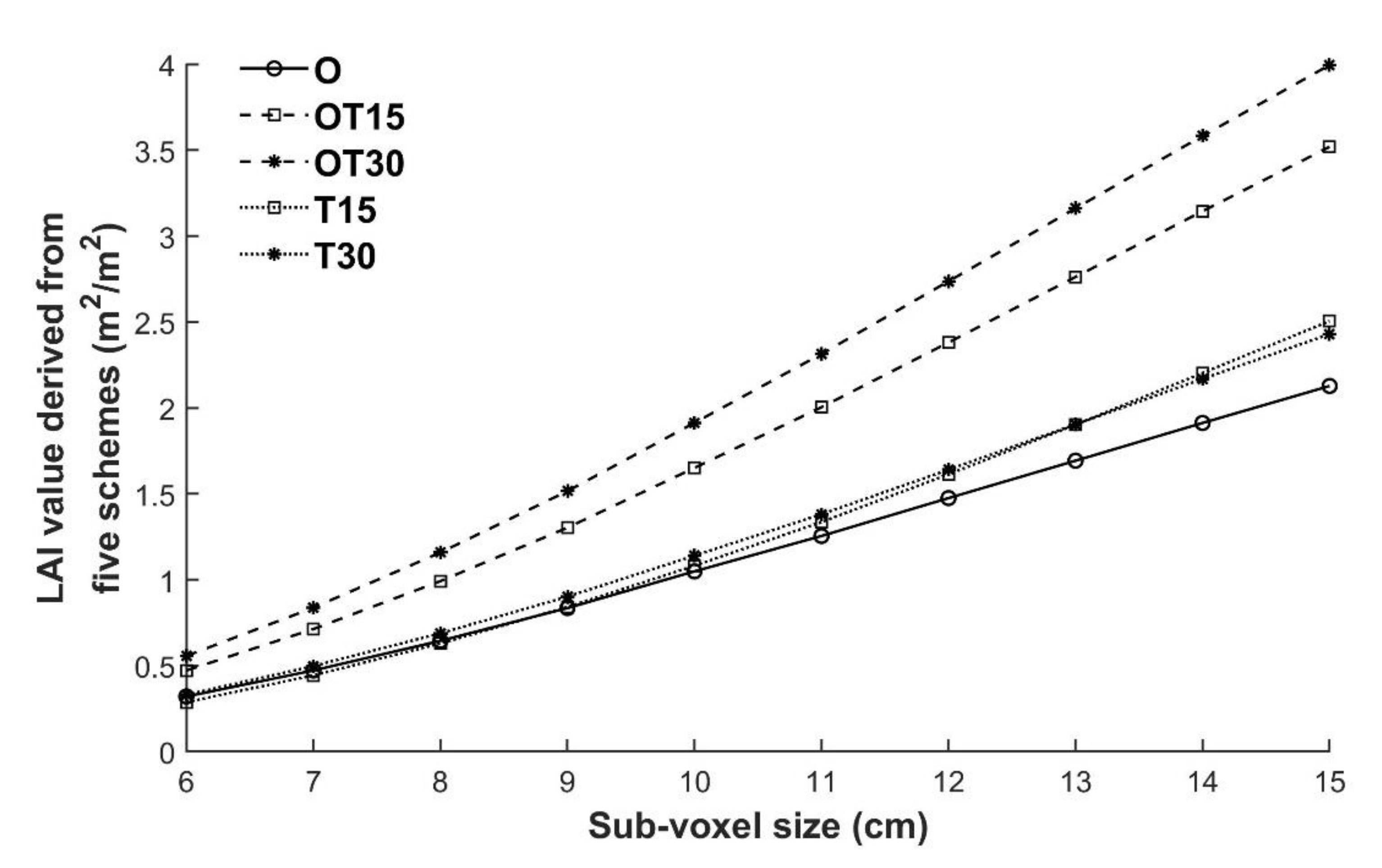
The derived LAI values were obtained from the 10-voxel models generated by each of the five schemes (Figure 7). Overall, the LAI derived from the five schemes increased with the increase in the sub-voxel size. For different voxelization models, OT30 always provided LAI estimates higher than O, OT15, T15 and T30. The LAI estimates provided by T15 and T30 were very close, and O always provided the lowest LAI estimate among the five schemes.
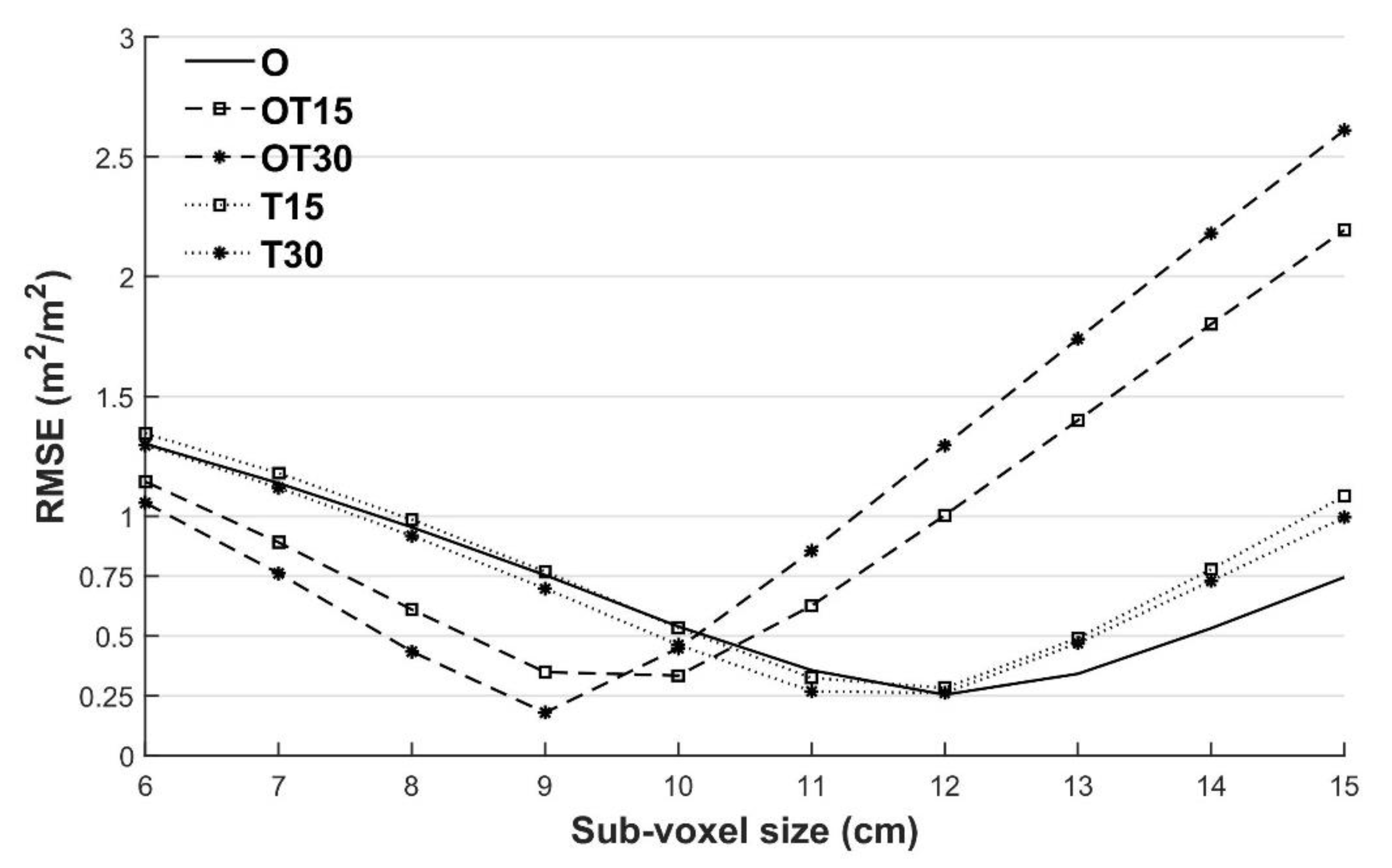
For the five schemes, the sub-voxel sizes corresponding to the slope a, intercept b, the highest R2 and the lowest RMSE of the linear fitting were explored. O, T15 and T30 give the best LAI estimates at the sub-voxel size of 0.12 m, while OT30 gives the best LAI estimates at the sub-voxel size of 0.09 m and OT15 gives the best LAI estimates at the sub-voxel size of 0.10 m (Table 1). This result is consistent with the RMSE result (sub-voxel size is 0.12 m: RMSE (O) = 0.2538 m2/m2, RMSE (T15) = 0.2824 m2/m2, RMSE (T30) = 0.2609 m2/m2; sub-voxel size is 0.10 m: RMSE (OT15) = 0.3333 m2/m2; sub-voxel size is 0.09 m: RMSE (OT30) = 0.1790 m2/m2) (Figure 8 and Table 2). Although the three single-angle schemes also provide good LAI estimation accuracy, the most suitable sub-voxel size is larger than that of OT15 and OT30. This shows that the completeness of O, T15 and T30 canopy information is lower than that of OT15 and OT30 (Figure 8).
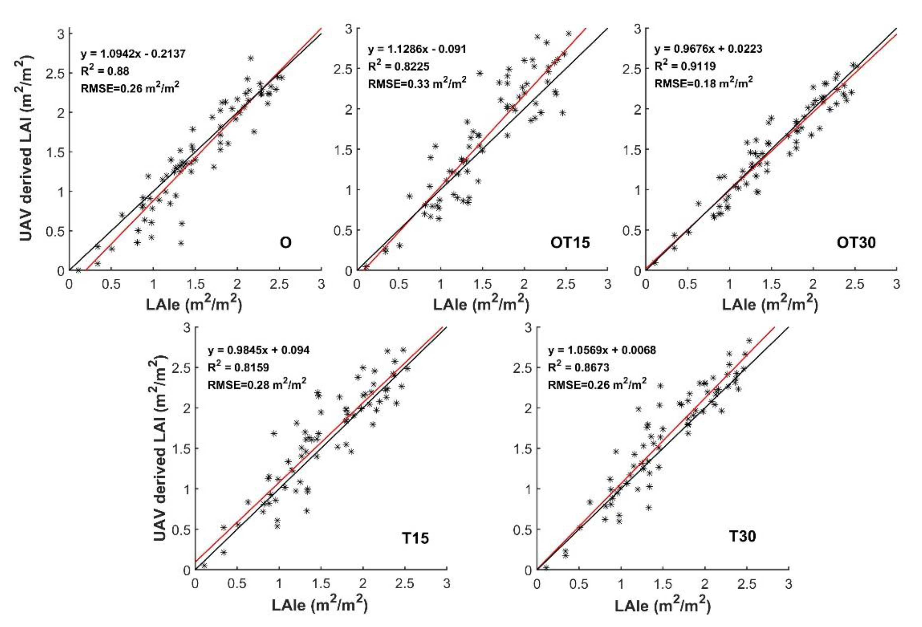
Each of the five schemes had a good linear fitting relationship with the LAI value measured on the field under the sub-voxel size that is most suitable for estimating LAI. The results of OT30 were stably distributed around Y = X, and its accuracy verification results are the best among all the schemes (Figure 9). The LAI values derived from the other four schemes had a relatively high degree of dispersion with the LAI values measured on field. Generally speaking, between the same kind of schemes, the LAI estimation provided by the multi-angle scheme was better than with the single-angle scheme (OT30 better than T30), and the LAI derived from adding the 30° photo was better than the one with the 15° photo (OT30 better than OT15; T30 better than T15) (Figure 9). However, the best LAI estimation accuracy of OT15 was worse than the other four schemes, which may be related to the poor image matching between the oblique photos of OT15.
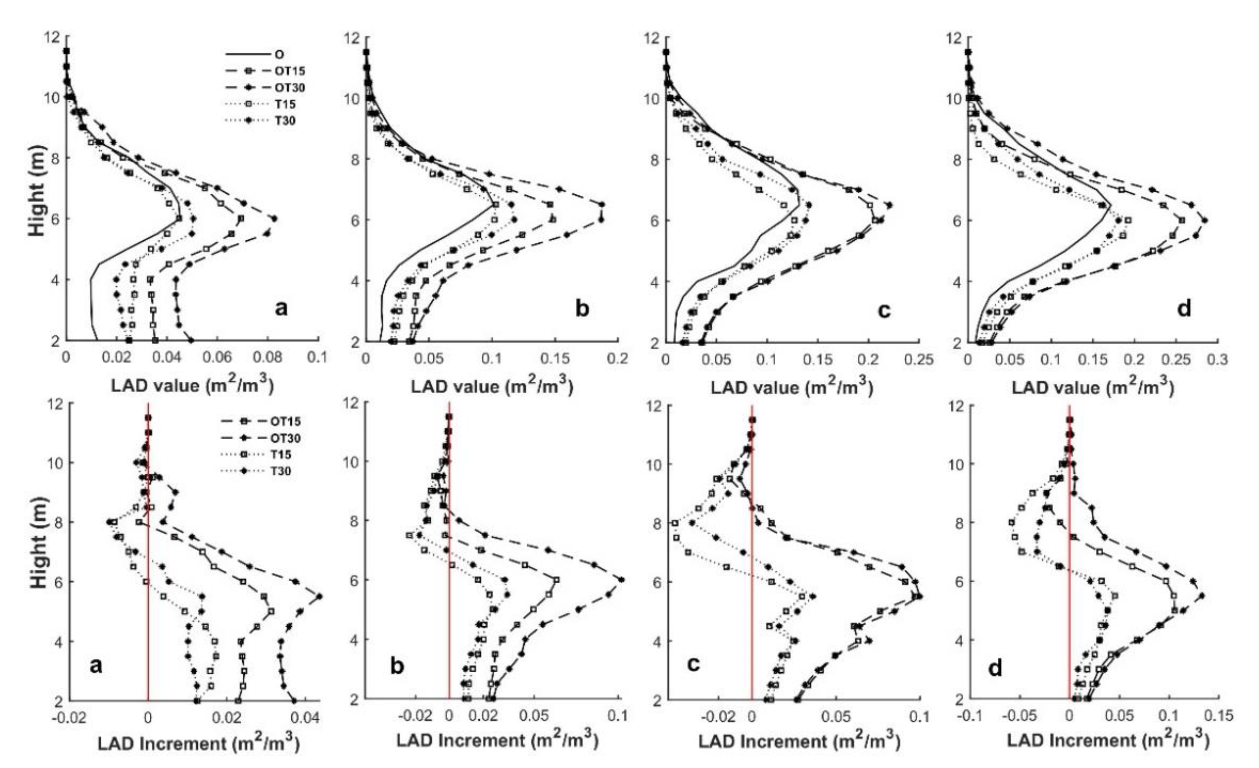
3.3. Leaf Area Distribution in Vertical Directions under the Same Sub-Voxel Size
To explore the structural integrity of the point cloud of five schemes at different heights and its influence on the overall LAI estimation of the canopy, the leaf area distribution at different heights of the canopy, namely the leaf area density (LAD), was compared under a same sub-voxel size. Then, scheme O was taken as a reference to further compare the LAD increments of the remaining four schemes at different heights. The vertical LAD distribution trends of the five schemes were very consistent with the morphological characteristics of the masson pine forest, but there was a large difference between the LAD values of the five schemes (Figure 10). The LAD estimate provided by the single tilt angle schemes (T15, T30) was always lower than the multiple angle schemes (OT15, OT30). In the middle and lower part of the canopy, T15, T30, OT15 and OT30 all gave leaf area estimates higher than O, but the LAD increments of these four schemes relative to O were not consistent in stands with different LAI values. Here, we divide the sample plots into four groups according to the value of LAI and calculate the LAD values and LAD increments of these four plans at different heights of the canopy relative to the O schemes (Figure 10). For the middle and lower part of the canopy, the LAD increment of the four schemes relative to O in the area where the LAI of 0.5–1.5 was more significant than that in the area with a LAI of 1.5–2.5. In the area where the LAI was 0.5–1.5, the LAD increment of the scheme with 30° photos was higher than that of the scheme with 15° photos, was not significant in the area where the LAI interval was 1.5–2. This shows that the acquisition for the lower part of the canopy from UAV gradually weakened with the increase of LAI and the decrease in the UAV lens angle. It is worth noting that T15 and T30 all showed a large decrease in LAD relative to O at the upper part of the canopy. This suggests that the point cloud density of O in the upper part of the canopy was higher than T15 and T30 and close to OT15 and OT30 (Figure 10).
4. Discussion
4.1. Three-Dimensional Reconstruction
Our research result was that coupling oblique photos and nadir photos can effectively improve the vertical coordinate accuracy of the point cloud. However, it is worth noting that under the premise of not using GCP, the height coordinate error provided by the scheme with nadir-photos-only reached 10.8 m (Figure 11), which is quite different from the results of other researchers [35,36,37]. The specific reason for this result is not clear, but it may be related to the camera calibration result or ground type, which can be further explored in future research. Even if there is still a coordinate error higher than the image resolution after point clouds registration, this degree of checkpoint error will not have much impact on the calculation of the canopy leaf area index on the plot scale. A large number of GCP can significantly improve the accuracy of point cloud coordinates [38]. However, setting a large number of GCPs in a complex forest scene is very difficult, and the low-cost advantages of the SFM–MVS process decrease as the GCP deployment points increase. Many studies have pointed out that coupling oblique photographs and nadiral photographs with RTK (without GCP) can also restore the surface model well in some complex scenes, which is consistent with the results of this study [39,40]. Restricted by the terrain and the coverage of the base station, RTK will produce large errors when applied to the coordinate acquisition of GCP under a forest that is heavily shaded by trees. Hence, based on our research results, in forest scenes, we recommend combining the nadir photo and the 30° tilted photo of the drone to obtain the canopy 3D point cloud.
In the SFM process, homology point-matching between images is the key step that directly determines the canopy 3D point-cloud density and the utilization of image information [41]. The result of homologous point matching between photos of different viewing angles changes and becomes unstable. Thus, a large number of oblique photos were used in this research to ensure the integrity of the canopy structure, which led to the point cloud derived from the multi-angle scheme being more refined and not having a large range of noise compared with the single-oblique angle schemes. In addition, lens resolution and flight height of UAV are also important factors that determine the density of derived point clouds [42]. Even if the high-resolution photos of drones flying at low altitudes are very effective in capturing canopy details [43], low content of photo content from a low flight altitude requires a high image overlap rate to get an excellent image matching result, while numerous photo sets generated in this way will greatly increase the cost of photogrammetry and computer hardware requirements. Thus, adjusting the UAV flight height according to lens resolution is very important for the reconstruction accuracy of the 3D model.
4.2. Leaf Area Estimation
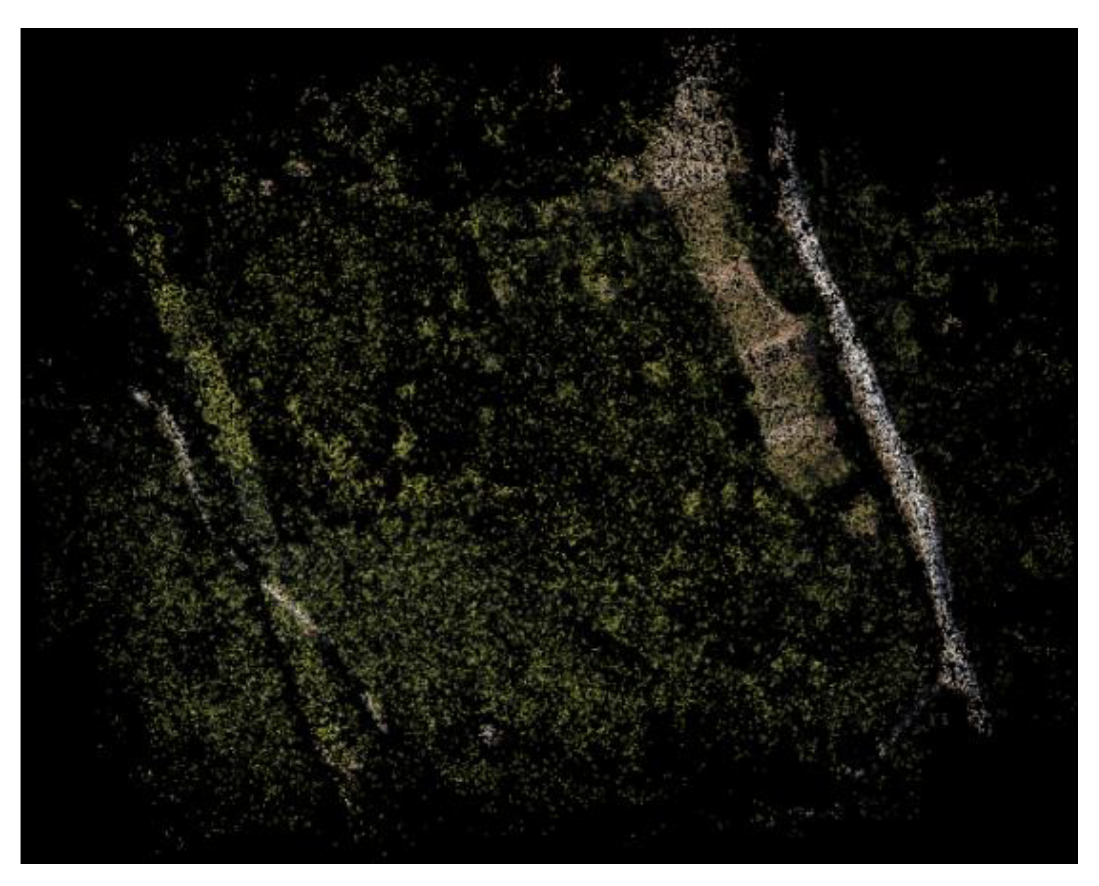
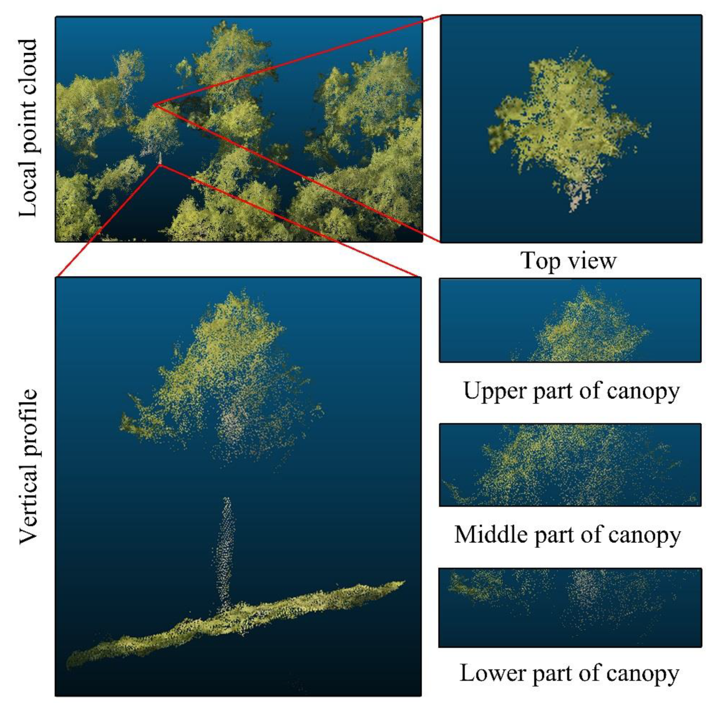
Numerous remote sensing estimation methods on forest LAI have been reported in the past [44,45], while the instability of multispectral data for model fitting and the high cost of LiDAR data have restricted forest LAI estimation. In this study, based on the SFM-MVS workflow, a 3D point cloud of the forest canopy was generated from a collection of photos from different angles of the drone, and the LAI was calculated based on the voxelized model. Our results show that the 3D point cloud derived from photogrammetry using nadir photos and 30° oblique photos provides the best LAI estimation. Although Lisein et al. [46] suggested that the canopy point cloud generated based on photogrammetry is incomplete because the optical image is not penetrating, they did not discuss the complement ability of oblique photography for canopy structure. Combining the LAD incremental comparison results of different oblique photography schemes relative to the nadir-photo-only scheme, we believe that coupling oblique photography and nadiral photography can compensate to a certain extent for the weak acquisition ability of the nadir-photo-only scheme for the canopy structure. Moreover, the UAV that executes the orthogonal flight plan can obtain canopy information from four directions, which further improves the canopy information obtained by oblique photography. Although detecting the complete canopy internal information is still difficult, oblique photography can obtain a very fine leaf point cloud for tree species with exposed leaves, which could avoid the overestimation of LAI caused by the existence of branches inside the canopy. The canopy structure of Masson pine in our study area is simple, and the leaves are relatively sparse due to poor soil [47], so the leaf information can be obtained very clearly and completely from the oblique image (Figure 12).
Sub-voxels of different sizes have different abilities to fill gaps in the point clouds [48]. The LAI estimation derived from the voxelization model increase with the increase of the sub-voxel size [49]. As long as the relatively complete canopy structure is retained, even point clouds with low density can also improve leaf area estimation by increasing the sub-voxel size (O, T15, T30). Therefore, the determination of the optimal sub-voxel size is extremely critical for forest leaf area estimation. However, the density of the point cloud derived from the nadir-photo only scheme (O) has a big difference in vertical space [50]. The point cloud derived from O is very fine due to excellent image details at the top of canopy but is sparse due to the limitation of nadir photo viewing angle in the middle and lower parts of the canopy. Thus, the good LAI estimation given by O is based on the fact that the voxels in the lower part of the canopy contain more blank areas in exchange, which determines that the nadir-photo-only scheme is not suitable for LAI estimation. The lower and middle structure of the two single-oblique angle schemes (T15, T30) is more complete than that of O. Nevertheless, the point cloud derived from oblique-only photos schemes is sparse and has many noise points because of the poor homology points matching results, which fail to reflect the details of canopy well. Thus, even if the sub-voxel size is increased to accommodate more blanks, the oblique-only photo schemes alone still can not give an accurate LAI estimate.
Multi-angle schemes combine the excellent image details of nadir photos for the top part of the canopy and the strong acquisition ability of oblique photos for the middle and lower canopy, which led to good performance in LAI estimation. The top and middle parts of the canopy are less affected by the canopy occlusion, so the multi-angle schemes in different LAI areas always provide a fairly accurate leaf area estimation. For the lower part of the canopy, the point cloud details become more complete as the angle of the oblique photo increases in the low-LAI area, which is not very significant in high-LAI areas because of the overlapping occlusions between canopies. In low-LAI areas, overlapping occlusions are rare because the lower part of the canopy is largely exposed due to the scarcity of trees, so the addition of oblique photos can significantly improve the LAD estimation of the middle and lower canopies. In the high-LAI area, the canopy overlap between the single wood blocks the lower canopy layer, so the UAV cannot get fine point clouds in this part of the canopy, which also leads to the underestimation of the leaf area under the canopy in the high LAI area.
4.3. Limitation of this Study
Since there are no real leaf area data for the lower part of the canopy, we cannot evaluate the LAD estimates for different heights of the canopy generated by the multi-angle scheme. Even though the LAD increment in this study is relative to the nadir-photo-only scheme, it can also reflect the improvement in leaf area estimation by point clouds derived from multi-angle schemes to a certain extent. In this study, we did not set up different altitude UAV flight plans to test their ability for forest LAI estimation, and the impact of increasing the resolution of the UAV camera on the estimation of LAI using point clouds generated from multi-angle images is also still unknown. Even if they are not the focus of this study, they may provide the potential for insufficient leaf area estimation in the lower part of the canopy in areas with canopy occlusion. Finally, obtaining sub-centimeter-level three-dimensional structures of the forest surface without using a large amount of GCP is one of the most important issues for future SFM–MVS applications in forest surveys.
5. Conclusions
Under the background that the SFM-MVS workflow technology is very mature, we explored the feasibility of using point cloud data derived from photogrammetry to estimate forest LAI. The results show that the scheme with oblique photos (OT15, OT30, T15, T30) always provides better checkpoint accuracy than schemes with nadir-photos only (O). For the four oblique photography schemes, the surface model accuracy of the multi-angle scheme (OT15 and OT30) is better than that of the single oblique angle scheme (T15 and T30). The point clouds data derived from the coupled nadir photos and 30° oblique photos provide the best checkpoint accuracy (RMSE (H) = 0.2917 m, RMSE (V) = 0.1797 m) and the best LAI estimation by sub-voxel size of 0.09 m (RMSE = 0.1790 m2/m2), and its improvement in the estimation of leaf area in the middle and lower part of the canopy is better than the single angle scheme (O, T15, T30) and the multi-angle solution with 15° oblique photos (OT15). Moreover, the LAI estimation provided by the scheme with 30° photos is always better than that of the scheme with 15° photos (T30 better than T15, OT30 better than OT15).
Author Contributions
Conceptualization, J.L. and K.Y.; methodology, L.L.; investigation, L.L., Y.D., Z.H., Y.C. and N.W.; data curation, L.L. and X.Y.; writing—original draft preparation, L.L.; writing—review and editing, J.L., Y.C.; project administration, J.L.; funding acquisition, J.L. and K.Y. All authors have read and agreed to the published version of the manuscript.
Funding
This research was funded by the National Key Research and Development Program of China, grant number: 2072YFD060010304, and National Natural Science Foundation of China, grant number: 31770760.
Institutional Review Board Statement
Not applicable.
Informed Consent Statement
Not applicable.
Data Availability Statement
The source codes developed in this study were donated to GitHub (https://github.com/TOTOROLLC/Forest-Stand-LAI-Remote-Sensing-Retrieval-Based-on-Photogrammetry (accessed on 7 January 2021)). And the data used to support the findings of this study are available from the corresponding author upon request.
Acknowledgments
This research was supported by the Forestry College of Fujian Agriculture and Forestry University. We are grateful to DJI Fujian Branch for teaching drone flight technology. We also appreciate Chunwang Cai for helping with the field investigation.
Conflicts of Interest
The authors declare no conflict of interest.
References
- Chen, J.M.; Chen, X.Y.; Ju, W.M.; Geng, X.Y. Distributed hydrological model for mapping evapotranspiration using remote sensing inputs. J. Hydrol. 2005, 305, 15–39. [Google Scholar] [CrossRef]
- Dietz, J.; Holscher, D.; Leuschner, C.; Hendrayanto, Y. Rainfall partitioning in relation to forest structure in differently managed montane forest stands in Central Sulawesi, Indonesia. Forest Ecol. Manag. 2006, 237, 170–178. [Google Scholar] [CrossRef]
- Cleugh, H.A.; Leuning, R.; Mu, Q.; Running, S.W. Regional evaporation estimates from flux tower and MODIS satellite data. Remote Sens. Environ. 2007, 106, 285–304. [Google Scholar] [CrossRef]
- Pierce, L.; Running, S. Rapid estimation of coniferous forest leaf area index using a portable integrating radiometer. Ecology 1988, 69, 1762–1767. [Google Scholar] [CrossRef]
- Hollinger, D.Y. Canopy organization and foliage photosynthetic capacity in a broad-leaved evergreen montane forest. Func. Ecol. 1989, 3, 53–62. [Google Scholar] [CrossRef]
- McWilliam, A.L.C.; Roberts, J.M.; Cabral, O.M.R.; Leitao, M.V.B.R.; Costa, A.C.L.; Maitelli, G.T.; Zamparoni, C.A.G.P. Leaf area index and above-ground biomass of terra firme rain forest and adjacent clearings in Amazonia. Func. Ecol. 1993, 7, 310–317. [Google Scholar] [CrossRef]
- Zheng, G.; Moskal, L.M. Retrieving leaf area index (LAI) using remote sensing: Theories, methods and sensors. Sensors 2009, 9, 2719–2745. [Google Scholar] [CrossRef] [PubMed] [Green Version]
- Baret, F.; Guyot, G. Potentials and limits of vegetation indices for LAI and APAR assessment. Remote Sens. Environ. 1991, 35, 161–173. [Google Scholar] [CrossRef]
- Wulder, M.A.; Ledrew, E.F.; Franklin, S.E.; Lavigne, M.B. Aerial image texture information in the estimation of northern deciduous and mixed wood forest leaf area index (LAI). Remote Sens. Environ. 1998, 64, 64–76. [Google Scholar] [CrossRef]
- Hosoi, F.; Omasa, K. Factors contributing to accuracy in the estimation of the woody canopy leaf area density profile using 3D portable lidar imaging. J. Exp. Bot. 2007, 58, 3463–3473. [Google Scholar] [CrossRef] [Green Version]
- Oshio, H.; Asawa, T.; Hoyano, A.; Miyasaka, S. Estimation of the leaf area density distribution of individual trees using high-resolution and multi-return airborne LiDAR data. Remote Sens. Environ. 2015, 166, 116–125. [Google Scholar] [CrossRef]
- Liu, Y.Z.; Fu, Y.J.; Zhou, P.X.; Zhuan, Y.H.; Zhong, K.J.; Guan, B.L. A real-time 3 D shape measurement with color texture using a monochromatic camera. Opt. Commun. 2020, 474, 126088. [Google Scholar] [CrossRef]
- Wright, D.; Dering, B.; Martinovic, J.; Gheorghiu, E. Neural responses to dynamic adaptation reveal the dissociation between the processing of the shape of contours and textures. Cortex 2020, 127, 78–93. [Google Scholar] [CrossRef] [PubMed]
- Grumpe, A.; Belkhir, F.; Wöhler, C. Construction of lunar DEMs based on reflectance modelling. Adv. Space Res. 2014, 53, 1735–1767. [Google Scholar] [CrossRef]
- Liu, W.C.; Wu, B.; Wöhler, C. Effects of illumination differences on photometric stereo shape-and-albedo-from-shading for precision lunar surface reconstruction. ISPRS J. Photogramm. Remote Sens. 2018, 136, 58–72. [Google Scholar]
- Wu, B.; Liu, W.C.; Grumpe, A.; Wöhler, C. Construction of pixel-level resolution DEMs from monocular images by shape and albedo from shading constrained with low-resolution DEM. ISPRS J. Photogramm. Remote Sens. 2018, 140, 3–19. [Google Scholar] [CrossRef]
- White, L.; Alfarhan, M.; Ahmed, T.; Aiken, C. Structural and orientation analysis of 3 D virtual outcrop models. Abstr. Progr. Geol. Soc. Am. 2008, 40, 423–424. [Google Scholar]
- Meinen, U.; Robinson, T. Mapping erosion and deposition in an agricultural landscape: Optimization of UAV image acquisition schemes for SfM-MVS. Remote Sens. Environ. 2020, 239, 111666. [Google Scholar] [CrossRef]
- Morgenroth, J.; Gomez, C. Assessment of tree structure using a 3 D image analysis technique—A proof of concept. Urban For. Urban Green. 2014, 13, 198–203. [Google Scholar] [CrossRef]
- Gatziolis, D.; Lienard, J.F.; Vogs, A.; Strigui, N.S. 3 D tree dimensionality assessment using photogrammetry and small unmanned aerial vehicles. PLoS ONE 2015, 10, e0137765. [Google Scholar] [CrossRef] [Green Version]
- Méndez-Barroso, L.A.; Zárate-Valdez, J.L.; Robles-Morúa, A. Estimation of hydromorphological attributes of a small forested catchment by applying the Structure from Motion (SfM) approach. Int. J. Appl. Earth Obs. Geoinf. 2018, 69, 186–197. [Google Scholar] [CrossRef]
- Peña-Villasenín, S.; Gil-Docampo, M.; Ortiz-Sanz, J. Professional SfM and TLS vs. a simple SfM photogrammetry for 3 D modelling of rock art and radiance scaling shading in engraving detection. J. Cult. Herit. 2019, 37, 238–246. [Google Scholar] [CrossRef]
- Zhang, X.J.; Zhao, P.C.; Hu, Q.W.; Ai, M.Y.; Hu, D.T.; Li, J.Y. A UAV-based panoramic oblique photogrammetry (POP) approach using spherical projection. ISPRS J. Photogram. Rem. Sens. 2020, 159, 198–219. [Google Scholar] [CrossRef]
- Aicardi, I.; Chiabrando, F.; Grasso, N.; Lingua, A.; Noardo, F.; Spano, A. UAV photogrammetry with oblique images: First analysis on data acquisition and processing. Int. Arch. Photogramm. Remote Sens. Spat. Inf. Sci. 2016, 41, 835–842. [Google Scholar] [CrossRef] [Green Version]
- Wu, B.; Xie, L.; Hu, H.; Zhu, Q.; Yau, E. Integration of aerial oblique imagery and terrestrial imagery for optimized 3 D modeling in urban areas. ISPRS J. Photogramm. Remote Sens. 2018, 139, 119–132. [Google Scholar] [CrossRef]
- Blanton, C.M.; Rockwell, T.K.; Gontz, A.; Kelly, J.T. Refining the spatial and temporal signatures of creep and co-seismic slip along the southern San Andreas Fault using very high resolution UAS imagery and SfM-derived topography, Coachella Valley, California. Geomorphology. 2020, 357, 107064. [Google Scholar] [CrossRef]
- Westoby, M.J.; Brasington, J.; Glasser, N.F.; Hambrey, M.J.; Reynolds, J.M. “Structure-from-Motion” photogrammetry: A low-cost, effective tool for geoscience applications. Geomorphology 2012, 179, 300–314. [Google Scholar] [CrossRef] [Green Version]
- Eltner, A.; Kaiser, A.; Castillo, C.; Rock, G.; Neugirg, F.; Abellán, A. Image-based surface reconstruction in geomorphometry–merits, limits and developments. Earth Surf. Dyn. 2016, 4, 359–389. [Google Scholar] [CrossRef] [Green Version]
- Shi, X.Y.; Peng, J.J.; Li, J.P.; Yan, P.T.; Gong, H.Y. The Iterative Closest Point Registration Algorithm Based on the Normal Distribution Transformation. Procedia Comput. Sci. 2019, 147, 181–190. [Google Scholar] [CrossRef]
- Zhang, W.; Qi, J.; Wan, P.; Wang, H.; Xie, D.; Wang, X.; Yan, G. An Easy-to-Use Airborne LiDAR Data Filtering Method Based on Cloth Simulation. Remote Sens. 2016, 8, 501. [Google Scholar] [CrossRef]
- Yang, A.X.; Wu, Z.Y.; Yang, F.L.; Su, D.P.; Ma, Y.; Zhao, D.N.; Qi, C. Filtering of airborne LiDAR bathymetry based on bidirectional cloth simulation. ISPRS J. Photogram. Rem. Sens. 2020, 163, 49–61. [Google Scholar] [CrossRef]
- Hosoi, F.; Omasa, K. Voxel-based 3-D modeling of individual trees for estimating leaf area density using high-resolution portable scanning lidar. IEEE Trans. Geosci. Remote Sens. 2006, 44, 3610–3618. [Google Scholar] [CrossRef]
- Weiss, M.; Baret, F.; Smith, G.J.; Jonckheere, I.; Coppin, P. Review of methods for in situ leaf area index (LAI) determination. Agric. For. Meteorol. 2004, 121, 37–53. [Google Scholar] [CrossRef]
- Lin, Y.; West, G. Retrieval of effective leaf area index (LAI) and leaf area density (LAD) profile at individual tree level using high density multi-return airborne LiDAR. Int. J. Appl. Earth Obs. Geoinf. 2016, 50, 150–158. [Google Scholar] [CrossRef]
- Ruzgienė, B.; Berteška, T.; Gečyte, S.; Jakubauskienė, E.; Aksamitauskas, V.Č. The surface modelling based on UAV Photogrammetry and qualitative estimation. Measurement 2015, 73, 619–627. [Google Scholar] [CrossRef]
- Mielcarek, M.; Kamińska, A.; Stereńczak, K. Digital Aerial Photogrammetry (DAP) and Airborne Laser Scanning (ALS) as Sources of Information about Tree Height: Comparisons of the Accuracy of Remote Sensing Methods for Tree Height Estimation. Remote Sens. 2020, 12, 1808. [Google Scholar] [CrossRef]
- Balenović, I.; Simic Milas, A.; Marjanović, H. A Comparison of Stand-Level Volume Estimates from Image-Based Canopy Height Models of Different Spatial Resolutions. Remote Sens. 2017, 9, 205. [Google Scholar] [CrossRef] [Green Version]
- Persia, M.; Barca, E.; Greco, R.; Marzulli, M.I.; Tartarino, P. Archival Aerial Images Georeferencing: A Geostatistically-Based Approach for Improving Orthophoto Accuracy with Minimal Number of Ground Control Points. Remote Sens. 2020, 12, 2232. [Google Scholar] [CrossRef]
- Thomas, O.; Stallings, C.; Wilkinson, B. Unmanned aerial vehicles can accurately, reliably, and economically compete with terrestrial mapping methods. J. Unmanned Veh. Syst. 2019, 8, 57–74. [Google Scholar] [CrossRef]
- Nolan, M.; Larsen, C.; Sturm, M. Mapping snow depth from manned aircraft on landscape scales at centimeter resolution using structure-from-motion photogrammetry. Cryosphere 2015, 9, 1445–1463. [Google Scholar] [CrossRef] [Green Version]
- Meesuk, V.; Vojinovic, Z.; Mynett, A.E. Extracting inundation patterns from flood watermarks with remote sensing SfM technique to enhance urban flood simulation: The case of Ayutthaya, Thailand. Comput. Environ. Urban. Syst. 2017, 64, 239–253. [Google Scholar] [CrossRef]
- D’Oleire-Oltmanns, S.; Marzolff, I.; Peter, K.D.; Ries, J.B. Unmanned aerial vehicle (UAV) for monitoring soil erosion in Morocco. Remote Sens. 2012, 4, 3390–3416. [Google Scholar] [CrossRef] [Green Version]
- Harwin, S.; Lucieer, A. Assessing the accuracy of georeferenced point clouds produced via multi-view stereopsis from Unmanned Aerial Vehicle (UAV) imagery. Remote Sens. 2012, 4, 1573–1599. [Google Scholar] [CrossRef] [Green Version]
- Pu, R.; Cheng, J. Mapping forest leaf area index using reflectance and textural information derived from WorldView-2 imagery in a mixed natural forest area in Florida, US. Int. J. Appl. Earth Obs. 2015, 42, 11–23. [Google Scholar] [CrossRef]
- Korhonen, L.; Korpela, I.; Heiskanen, J.; Maltamo, M. Airborne discrete-return LIDAR data in the estimation of vertical canopy cover, angular canopy closure and leaf area index. Remote Sens. Environ. 2011, 115, 1065–1080. [Google Scholar] [CrossRef]
- Lisein, J.; Pierrot-Deseilligny, M.; Bonnet, S.; Lejeune, P. A Photogrammetric Workflow for the Creation of a Forest Canopy Height Model from Small Unmanned Aerial System Imagery. Forests 2013, 4, 922–944. [Google Scholar] [CrossRef] [Green Version]
- Yu, K.Y.; Yao, X.; Deng, Y.B.; Lai, Z.J.; Lin, L.C.; Liu, J. Effects of stand age on soil respiration in Pinus massoniana plantations in the hilly red soil region of Southern China. Catena 2019, 178, 313–321. [Google Scholar] [CrossRef]
- Morsdorf, F.; Kötz, B.; Meier, E.; Itten, K.I.; Allgöwer, B. Estimation of LAI and fractional cover from small footprint airborne laser scanning data based on gap fraction. Remote Sen. Environ. 2006, 104, 50–61. [Google Scholar] [CrossRef]
- Deng, Y.; Yu, K.; Yao, X.; Xie, Q.; Hsieh, Y.; Liu, J. Estimation of Pinus massoniana Leaf Area Using Terrestrial Laser Scanning. Forests 2019, 10, 660. [Google Scholar] [CrossRef] [Green Version]
- Seifert, E.; Seifert, S.; Vogt, H.; Drew, D.; van Aardt, J.; Kunneke, A.; Seifert, T. Influence of Drone Altitude, Image Overlap, and Optical Sensor Resolution on Multi-View Reconstruction of Forest Images. Remote Sens. 2019, 11, 1252. [Google Scholar] [CrossRef] [Green Version]
Figure 1.
Distribution of sample plots.

Figure 2.
Unmanned aerial vehicle (UAV) orthogonal flight plan.

Figure 3.
General workflow.

Figure 4.
Homologous point matching result.

Figure 5.
Schematic diagram of Leaf Area Index (LAI) field measurement scheme. The red line is the boundary of the sample plot, the black spot is the measuring station and the fan-shaped area is the orientation of LAI-2200 canopy analyzer probe rod.
Figure 5.
Schematic diagram of Leaf Area Index (LAI) field measurement scheme. The red line is the boundary of the sample plot, the black spot is the measuring station and the fan-shaped area is the orientation of LAI-2200 canopy analyzer probe rod.

Figure 6.
Boxplots describe the checkpoint absolute errors of the five schemes before and after point cloud registration in vertical and horizontal directions. Before point clouds registration (a1: horizontal direction; a2: vertical direction); after point clouds registration (b1: horizontal direction; b2: vertical direction).

Figure 7.
The distribution trend of average LAI of 72 plots derived from voxel model with different sub-voxel sizes (6 cm–15 cm, step is 1 cm).
Figure 7.
The distribution trend of average LAI of 72 plots derived from voxel model with different sub-voxel sizes (6 cm–15 cm, step is 1 cm).

Figure 8.
Root-mean-square error (RMSE) between the LAI derived from five schemes and effective leaf area index (LAIe) under different sub-voxel sizes.
Figure 8.
Root-mean-square error (RMSE) between the LAI derived from five schemes and effective leaf area index (LAIe) under different sub-voxel sizes.

Figure 9.
The best LAI estimation scheme for each of the five schemes, under different sub-voxel sizes. Sub-voxel size when the LAI of the five schemes was the best: O (0.12 m); OT15 (0.10 m); OT30 (0.09 m); T15 (0.12 m); T30 (0.12 m).
Figure 9.
The best LAI estimation scheme for each of the five schemes, under different sub-voxel sizes. Sub-voxel size when the LAI of the five schemes was the best: O (0.12 m); OT15 (0.10 m); OT30 (0.09 m); T15 (0.12 m); T30 (0.12 m).

Figure 10.
In areas with different LAI levels, the leaf area density (LAD) distribution and the LAD increment relative to O of five schemes at different heights from ground (sub-voxel size is 0.09 m). a is the area with LAI interval 0.5–1, b is the area with LAI interval 1–1.5, c is the area with LAI interval 1.5–2, d is the area with LAI interval 2–2.5.

Figure 11.
The side view intuitively reflects the height difference between the surface model of O and OT30, where the colored area is OT30 and the gray area is O.
Figure 11.
The side view intuitively reflects the height difference between the surface model of O and OT30, where the colored area is OT30 and the gray area is O.

Figure 12.
Figure shows the local point cloud of OT30 and the vertical profile distribution of a single tree. For better display, the ground point clouds are removed.
Figure 12.
Figure shows the local point cloud of OT30 and the vertical profile distribution of a single tree. For better display, the ground point clouds are removed.


Table 1.
Linear fitting results between the LAI derived from five schemes under different sub-voxel sizes and LAIe (a is slope, b is intercept and R2 is the square of correlation coefficient).
Table 1.
Linear fitting results between the LAI derived from five schemes under different sub-voxel sizes and LAIe (a is slope, b is intercept and R2 is the square of correlation coefficient).
| O | OT15 | OT30 | T15 | T30 | |||||||||||
|---|---|---|---|---|---|---|---|---|---|---|---|---|---|---|---|
| Sub-Voxel Size (m) | a | b | R2 | a | b | R2 | a | b | R2 | a | b | R2 | a | b | R2 |
| 0.06 | 0.25 | −0.06 | 0.87 | 0.34 | −0.05 | 0.82 | 0.37 | −0.01 | 0.91 | 0.19 | 0.00 | 0.83 | 0.23 | −0.02 | 0.87 |
| 0.07 | 0.36 | −0.09 | 0.87 | 0.51 | −0.07 | 0.82 | 0.55 | −0.01 | 0.91 | 0.29 | 0.00 | 0.82 | 0.34 | −0.03 | 0.87 |
| 0.08 | 0.49 | −0.11 | 0.87 | 0.70 | −0.08 | 0.82 | 0.75 | 0.00 | 0.91 | 0.40 | 0.01 | 0.82 | 0.46 | −0.03 | 0.87 |
| 0.09 | 0.63 | −0.14 | 0.88 | 0.90 | −0.09 | 0.82 | 0.97 | 0.02 | 0.91 | 0.53 | 0.02 | 0.82 | 0.60 | −0.02 | 0.87 |
| 0.10 | 0.79 | −0.17 | 0.88 | 1.13 | −0.09 | 0.82 | 1.21 | 0.05 | 0.91 | 0.68 | 0.04 | 0.82 | 0.75 | −0.02 | 0.87 |
| 0.11 | 0.94 | −0.19 | 0.88 | 1.35 | −0.08 | 0.82 | 1.43 | 0.10 | 0.91 | 0.83 | 0.06 | 0.82 | 0.90 | 0.00 | 0.87 |
| 0.12 | 1.09 | −0.21 | 0.88 | 1.58 | −0.06 | 0.82 | 1.67 | 0.17 | 0.90 | 0.98 | 0.09 | 0.82 | 1.05 | 0.02 | 0.87 |
| 0.13 | 1.25 | −0.23 | 0.88 | 1.81 | −0.02 | 0.82 | 1.89 | 0.24 | 0.90 | 1.14 | 0.14 | 0.81 | 1.20 | 0.05 | 0.87 |
| 0.14 | 1.40 | −0.25 | 0.88 | 2.02 | 0.03 | 0.81 | 2.11 | 0.33 | 0.90 | 1.31 | 0.18 | 0.81 | 1.35 | 0.09 | 0.86 |
| 0.15 | 1.54 | −0.26 | 0.88 | 2.22 | 0.09 | 0.81 | 2.31 | 0.43 | 0.89 | 1.47 | 0.24 | 0.81 | 1.49 | 0.13 | 0.86 |
Table 2.
Root-mean-square error (RMSE) (m2/m2) between the LAI derived from five schemes and LAIe under different sub-voxel sizes.
Table 2.
Root-mean-square error (RMSE) (m2/m2) between the LAI derived from five schemes and LAIe under different sub-voxel sizes.
| Sub-Voxel Size (m) | RMSE (m2/m2) | ||||
|---|---|---|---|---|---|
| O | OT15 | OT30 | T15 | T30 | |
| 0.06 | 1.3009 | 1.1429 | 1.0558 | 1.3437 | 1.2954 |
| 0.07 | 1.1370 | 0.8897 | 0.7603 | 1.1786 | 1.1176 |
| 0.08 | 0.9529 | 0.6093 | 0.4334 | 0.9844 | 0.9168 |
| 0.09 | 0.7531 | 0.3480 | 0.1790 | 0.7671 | 0.6967 |
| 0.10 | 0.5386 | 0.3333 | 0.4471 | 0.5323 | 0.4617 |
| 0.11 | 0.3558 | 0.6249 | 0.8542 | 0.3243 | 0.2677 |
| 0.12 | 0.2538 | 1.0027 | 1.2946 | 0.2824 | 0.2609 |
| 0.13 | 0.3410 | 1.3995 | 1.7398 | 0.4890 | 0.4691 |
| 0.14 | 0.5309 | 1.8011 | 2.1802 | 0.7770 | 0.7286 |
| 0.15 | 0.7443 | 2.1943 | 2.6115 | 1.0836 | 0.9948 |
Publisher’s Note: MDPI stays neutral with regard to jurisdictional claims in published maps and institutional affiliations. |
© 2021 by the authors. Licensee MDPI, Basel, Switzerland. This article is an open access article distributed under the terms and conditions of the Creative Commons Attribution (CC BY) license (http://creativecommons.org/licenses/by/4.0/).
Share and Cite
MDPI and ACS Style
Lin, L.; Yu, K.; Yao, X.; Deng, Y.; Hao, Z.; Chen, Y.; Wu, N.; Liu, J. UAV Based Estimation of Forest Leaf Area Index (LAI) through Oblique Photogrammetry. Remote Sens. 2021, 13, 803. https://0-doi-org.brum.beds.ac.uk/10.3390/rs13040803
AMA Style
Lin L, Yu K, Yao X, Deng Y, Hao Z, Chen Y, Wu N, Liu J. UAV Based Estimation of Forest Leaf Area Index (LAI) through Oblique Photogrammetry. Remote Sensing. 2021; 13(4):803. https://0-doi-org.brum.beds.ac.uk/10.3390/rs13040803
Chicago/Turabian StyleLin, Lingchen, Kunyong Yu, Xiong Yao, Yangbo Deng, Zhenbang Hao, Yan Chen, Nankun Wu, and Jian Liu. 2021. "UAV Based Estimation of Forest Leaf Area Index (LAI) through Oblique Photogrammetry" Remote Sensing 13, no. 4: 803. https://0-doi-org.brum.beds.ac.uk/10.3390/rs13040803
Note that from the first issue of 2016, this journal uses article numbers instead of page numbers. See further details here.