Crop Biomass Mapping Based on Ecosystem Modeling at Regional Scale Using High Resolution Sentinel-2 Data

Abstract

We evaluate the potential of using a process-based ecosystem model (BEPS) for crop biomass mapping at 20 m resolution over the research site in Manitoba, western Canada driven by spatially explicit leaf area index (LAI) retrieved from Sentinel-2 spectral reflectance throughout the entire growing season. We find that overall, the BEPS-simulated crop gross primary production (GPP), net primary production (NPP), and LAI time-series can explain 82%, 83%, and 85%, respectively, of the variation in the above-ground biomass (AGB) for six selected annual crops, while an application of individual crop LAI explains only 50% of the variation in AGB. The linear relationships between the AGB and these three indicators (GPP, NPP and LAI time-series) are rather high for the six crops, while the slopes of the regression models vary for individual crop type, indicating the need for calibration of key photosynthetic parameters and carbon allocation coefficients. This study demonstrates that accumulated GPP and NPP derived from an ecosystem model, driven by Sentinel-2 LAI data and abiotic data, can be effectively used for crop AGB mapping; the temporal information from LAI is also effective in AGB mapping for some crop types.

1. Introduction

Biomass is the organic matter produced by plants and animals with accumulated energy directly or indirectly from photosynthesis. Within botanic biomass, agricultural biomass is characterized by two major types, food-based crops and non-food-based crops, albeit with no clear boundaries between these categories. In the following, we briefly review the biomass mapping methods based on remote sensing data for two major grain-crops, oil and starch crops, within the category of food-based crops.

The methodologies for biomass mapping of herbaceous grain crops are also applicable to energy crops. Ahamed et al. [1] extensively reviewed remote sensing methods for biomass mapping for feedstock production with a focus on using various vegetation indices (VIs), biophysical and biochemical variables, such as leaf area index (LAI, or L) and chlorophyll content. Recently, Chao et al. [2] categorized the methods for biomass mapping of energy crops into five types: VI-based simple statistical analysis, Synthetic Aperture Radar (SAR) backscatter-based analysis, Net Primary Productivity (NPP) models with remote sensing data as inputs, the crop height-based method, and crop growth models with remote sensing inputs.

Here, we simplify these methods into two categories: plant trait-based methods and photosynthesis-based methods. Plant trait-based methods relate crop biophysical parameters such as LAI, height and/or canopy chlorophyll content, at a critical time (e.g., maximum values in the growing season), to plant biomass. Essentially, various VIs [3,4,5,6] are often used to approximate the maximum photosynthetic capacity of a crop canopy in the growing season in order to estimate the end-of-season biomass. The approach does not consider the effect of abiotic factors, such as soil properties and meteorological variables, on biomass accumulation. The capacity of these indices to track biomass changes is reduced when crops begin to senesce as these VIs are not sensitive to non-green biomass. Unmanned aerial vehicle (UAV) [7,8,9] or Lidar-derived crop height [10] relates to crop volume or biomass during vegetative stages but this approach is unable to track increases in biomass at reproductive stages when crop height is relatively stable. SAR-based methods relate the crop volume-scattering with biomass [11], but they are affected by uncertainties related to soil moisture and canopy water content contributions to scattering, especially before harvest [12]. Therefore, plant trait-based methods can be more effective in tracking crop biomass accumulation during vegetative growth stages. The use of multi-temporal data can mitigate the above-mentioned limitations, as the envelope of LAI time series contains information on crop growing season, e.g., the amount of accumulated heat units [13,14].

In contrast, photosynthesis-based methods track the accumulation of biomass beyond vegetative accumulation and into reproductive stages [15]. These methods take into consideration both biotic and abiotic impacts on crop growth and therefore, are less prone to the saturation problems than plant trait-based methods. Both light use efficiency (LUE) models [16,17,18,19] and mechanistic enzymatic ecosystem models (such as DSSAT [20] and EPIC [21]) belong to this category. A crop growth model can be based on either LUE models or enzymatic ecosystem process models, but with additional modules and parameters describing the crop phenological developments and carbon allocations [22]. Photosynthetic models are especially useful for tracking the accumulation of above-ground biomass (AGB) of annual crops as the AGB is accumulated from crop emergence. The use of photosynthetic models for crop biomass estimation also has a sound mechanism: Schlesinger [23] noted that the carbon (C) content of biomass is almost always between 45 and 50% per unit weight; therefore, the photosynthesis-based method relates C assimilation to the total amount of crop biomass accumulation. Crop growth models rely on numerous inputs of plant traits which are often unavailable for large-scale applications. Assimilation of satellite spectral information [24] or satellite-derived plant biophysical parameters [25,26] into crop growth models can help improve the accuracy of biomass mapping [27].

In addition to methodological advancements, research on crop biomass retrieval using optical satellite images has evolved from low to high spatial resolutions, e.g., from 1 km AVHRR [27], 250 m MODIS [28], 30 m Landsat [29], 10 m Sentinel-2 [30], 6.5 m RapidEye [31] and sub-meter UAV [7]. Particularly, the Sentinel-2 A and B missions operated by the European Space Agency’s Copernicus Programme acquires data in 13 optical bands at resolutions from 60 to 10 m, and with a 5-day revisit. This twin satellites constellation offers nearly global coverage and the data are free and open. As such, Sentinel-2 is an important source of data for operational agricultural monitoring, as well as biomass and yield mapping [32]. Although VI-based methods are used widely for biomass mapping [30,33,34,35], integration of multi-temporal Sentinel-2 and abiotic information into photosynthetic models can outperform these VI methods for crop biomass mapping [32,36].

The objective of this study is to demonstrate capabilities and evaluate the performance of an ecosystem model to simulate annual crop gross primary production (GPP) and NPP for the purpose of crop AGB estimation at a regional scale using high-resolution Sentinel-2 data. To achieve this objective, Sentinel-2 reflectance data are used to derive time-series LAI as an input to the ecosystem model. These LAI maps, along with other abiotic variables, are integrated to simulate crop GPP and NPP (Section 2). The correlations between simulated GPP, NPP and measured AGB for several crops are examined in Section 3; the correlation between AGB and individual LAI or LAI time-series is also examined. The uncertainties of GPP and NPP simulations for crop biomass mapping are discussed in Section 3. Section 4 summarizes the key conclusions.

2. Materials and Methods

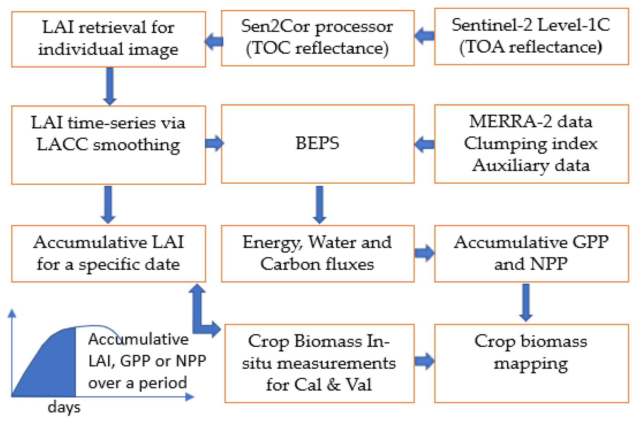
2.1. Ecosystem Model for Crop GPP and NPP Simulation

The Boreal Ecosystems Productivity Simulator (BEPS) is used to simulate crop GPP and NPP in this study [37,38]. BEPS has been developed since 1997 and has evolved from a daily version [38] to the current hourly version [39], with process-based modules to simulate water, energy and carbon budgets [40,41]. Although BEPS was initially developed for boreal ecosystems, it has been evolved and expanded to cover temperate and tropical ecosystems at regional and global scales [42,43,44,45,46] and has been re-structured for parallel computation and data assimilation [46,47,48]. BEPS has also been used for estimations of winter wheat yield in China [49] and cotton yield in the US [50], as C3 plants share the same enzymatic mechanism-based photosynthesis theory at the leaf-level, i.e., Farquhar’s leaf-level biochemical model [51], and BEPS has a “two-leaf” approach [52] to upscale the ecosystem GPP to canopy-level for various ecosystems including crops [38]. NPP is then modeled as the difference between photosynthesis (GPP) and autotrophic respiration. BEPS has the mechanism to simulate CO₂ fertilization, using CO₂ concentration data from https://www.esrl.noaa.gov/gmd/ccgg/trends/global.html (accessed on 20 July 2019).

The maximum rate of Rubisco carboxylation (V_cmax) of crops varies with cultivars and nutrition condition. Although BEPS has the model structure to assimilate a dynamic variable V_cmax, the V_cmax values are fixed at 120 µmoL m⁻² s⁻¹ for different crops in this study, to be consistent with our previous crop modeling work [48], since pixel-level V_cmax measurements are currently unavailable at the spatial resolution of Sentinel-2.

The C4 plants have less photorespiration and are more efficient in photosynthesis although their leaf V_cmax is low, e.g., at 40 ± 1 μmoL m⁻² s⁻¹ [53] for maize (corn). Since BEPS has no C4 module, we test if the increase in V_cmax to 120 µmoL m⁻² s⁻¹ for C4 corn using a C3 model could partially compensate the underestimation of GPP simulation due to the lack of a photorespiration module for the purpose of corn biomass mapping.

2.2. The Link between Carbon Fluxes and Biomass

In this study, BEPS uses daily LAI and hourly meteorological data as inputs and outputs GPP and NPP for each hour (g C m⁻² h⁻¹); the hourly GPP and NPP are then binned into daily scale in units of g C m⁻² day⁻¹. Using GPP as an example, the accumulative GPP in unit of g C m⁻² on a specific day is defined as the sum of daily GPP from day 1 to day n:

$$GP{P}_A={{\displaystyle \sum }}_{i=1}^{n}GP{P}_i$$

(1)

where GPP_A is also referred to as GPP for simplicity, hereafter; GPP_i is the daily total GPP for day i; day 1 is defined as the first day when LAI is larger than 0.

As summarized in the Introduction, there is justification to link crop GPP to crop biomass. Given an accumulated crop GPP (g C m⁻²) simulated by the BEPS over a given period of time in the growing season, the accumulated crop biomass (B, in units of g m⁻²) in the same period is estimated as:

$$B=GPP·c_1·c_2$$

(2)

where c₁ is the carbon use efficiency (CUE, the ratio of NPP to GPP) and ranges from 0 to 1 for different species [54]; CUE is often set to 0.5 as an average for global ecosystems [55]; c₂ is the biomass to carbon ratio. As summarized by Schlesinger [23], the C content of biomass is almost always found to be between 45 and 50%; therefore, c₂ is close to 2.0.

As CUE increases with a decrease in temperature [56,57], CUE in high latitudes is above 0.5. Since c₂ is slightly larger than 2.0, the product of c₁ and c₂ is expected to be larger than 1.0 in high latitudes. Given the small variations in c₁ and c₂ in a specific area, it is desirable to directly link GPP to biomass by a single coefficient C for practical applications:

$$B=GPP·C$$

(3)

Equation (3) assumes a linear relationship between GPP and biomass. The correlation coefficient between GPP and AGB for a few crop types will be examined since only AGB data are available in this study.

Based on Equations (2) and (3), crop yield (Y, in unit of Kg Ha⁻¹) can also be estimated from the end-of-season crop GPP, although it is not the focus of this study:

$$Y=GPP·c_1·c_2·c_3·c_4$$

(4)

where c₃ is the harvest index (HI), the ratio of harvested grain mass to total aboveground dry biomass; and c₄ is 10, the factor to convert the unit from g m⁻² to kg to Ha⁻¹. As reported by Lambert, Traoré, Blaes, Baret and Defourny [30], the AGB explains more variations in crop yield than the peak LAI values.

Similarly, we also compare crop biomass to accumulated LAI or NPP in a period in order to test their correlations. Accumulated LAI is defined as the sum of daily LAI from the date when LAI is larger than zero to a specific date in the growing season; the daily LAI is interpolated from remote sensed derived LAI. Similar to GPP, NPP and accumulated LAI also contain information from a time series rather than a single measurement.

To estimate AGB from NPP:

$$AGB=NPP·c_2·c_5$$

(5)

where c₅ is ratio of AGB to total biomass. c₅ may vary with different crops and can be calibrated; in this study, c₅ is set to as 80%.

A full diagram of the data processing flow is illustrated in Figure 1.

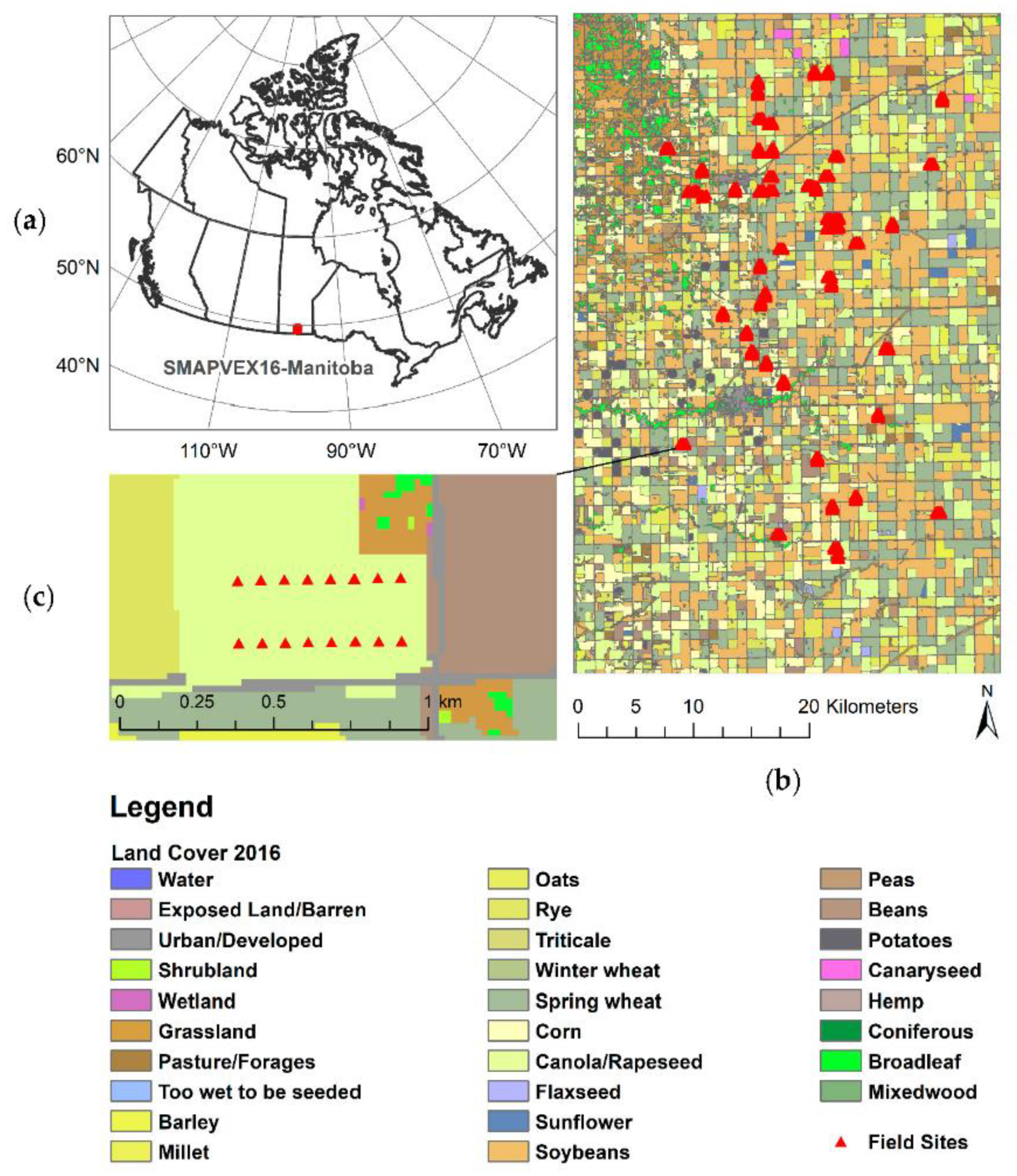
2.3. Crop LAI and Above-Ground Biomass Collection from the SMAPVEX16-MB Field Campaign

In this study, ground measurements of AGB are from the SMAP Validation Experiment 2016 in the Carman/Elm Creek region of southern Manitoba, Canada (SMAPVEX16-MB). This experiment was conducted to support NASA’s SMAP satellite post-launch calibration/validation activities [58]. Figure 2 shows the location of the SMAPVEX16-MB experiment and the distribution of the AGB sampling plots. A total of 50 fields were selected for sampling in this campaign, with each field covering an area of 800 m × 800 m. These 50 fields represent the dominant crops within the study area. According to the AAFC Annual Crop Inventory, soybeans, spring wheat and canola accounted for approximately 70% of crops grown in the study area, with corn, oats, and other field beans accounting for approximately 17% of the study area in 2016. These sites are within a region of approximately 26 km × 48 km.

Field sampling was conducted on 13 different dates, 13, 15, 18, 20, 27, and 28 June and 5, 6, 11, 12, 17, 20, and 21 July. Each field had 16 sampling locations for soil moisture, although data on crop vegetation were collected from only 6 of these sites (Locations 2, 3, 10, 11, 13 and 14). The objective during SMAPVEX16-MB was to collect crop data approximately once per week during the experiment. Given this goal, each field was sampled 5 times for the purpose of characterizing crop growth. This strategy resulted in 380 data points to be compared with GPP simulated at 20 m resolution from Sentinel-2 data.

During sampling, all above-ground crop biomass was cut at the soil surface, placed in plastic bags to prevent water loss, and immediately transported to a portable field lab for weighing. For crops with wide row spacing (corn and beans), 5 plants were harvested in each of two rows. Biomass (g) per unit area (m²) was determined using wet and dry weights and plant density. For narrowly placed crops (canola, oats and wheat), all biomass was collected within a 0.5 x 0.5 m square. After wet weights were determined, plants were transported to a drying room. Here plants were left for approximately one week, until stable dry weights determined that plants had completely dried. The weights of these samples were further calibrated using samples dried by an oven (60 °C for 48 h). This dataset includes samples for six crop types, i.e., oat, soybean, wheat, corn, canola and black bean. A complete description of biomass collection is detailed at https://nsidc.org/data/SV16M_V/versions/1 (accessed on 30 July 2019) and by Bhuiyan, McNairn, Powers, Friesen, Pacheco, Jackson, Cosh, Colliander, Berg, Rowlandson, Bullock and Magagi [58].

The water content of plant organs varies with specific crop type and seasons; after the gross biomass is dried, the dry matter can be directly compared to the BEPS simulation of the net carbon assimilation.

Along with biomass measurements, LAI was measured with hemispherical digital photos [59]. In this technique, a camera with a fish-eye lens captured photos of the crop canopy with the camera positioned at least 50 cm above or below the canopy. The camera was mounted on a pole if the picture was taken above the canopy. Seven photos were taken along two transects (14 photos in total) at three sampling sites for each of the fields. Crews were instructed to take one photo then move approximately 5 m to take the next photos. Field crews positioned themselves relative to the sun to minimize shadowing in the photos. These photos were post-processed to estimate LAI using the CanEye software. All 14 photos were averaged to provide one estimate of LAI per sample site. Prior to the use of CanEye, the photos were enhanced to increase the quality through the use of ViewNX-2 (Nikon) software. Once enhancements were implemented, the images were then imported in the CanEye software for classification and LAI calculation. The parameters of the software were configured in accordance with the photos, i.e., number of lines and columns, julian date and latitude. Masking for any non-soil or data acquisition anomalies were applied where necessary in addition to any removal of photos that were problematic.

In the data processing, all green leave, stems, and spikelets are included. Since the measurements were taken in summer, the plants did not senescence at the time of measurements. Therefore, the ground LAI measurements include total green elements. This corresponds well to Sentinel-2-derived LAI as the simple ratio index is sensitive to all elements with chlorophyll pigments.

2.4. Key Input Data for BEPS Simulation

Sentinel-2 Level-1C top-of-atmosphere (TOA) reflectance products are used to derive LAI. These products are organized into tiles of 100 by 100 km² in UTM projection and WGS84 ellipsoid and are available from the Copernicus Open Access Hub (https://scihub.copernicus.eu/dhus/#/home (accessed on 1 June 2019)). Two tiles (14UNA and 14UNV) covering the SMAPVEX16-MB region were selected and mosaicked. For BEPS simulation, a region of approximately 40 km × 60 km is subset to match the region shown in Figure 2.

The Sen2Cor atmospheric correction processor [60] is used to convert the TOA reflectance to top-of-canopy (TOC) reflectance, i.e., Sentinel-2 Level-2A product. A Simple Ratio index (SR), defined as a ratio of near-infrared band to red band reflectances (or band 8A to band 4 reflectances from Sentinel-2) was used to derive LAI at 20 m resolution, while taking into account the effect of bidirectional reflectance distribution [61]. We chose band 8A in 20 m resolution rather than band 8 in 10 m resolution because band 8A is more sensitive to LAI.

In [61], the LAI is modeled as

L = f (SR ∗ f_BRDF (θ_s, θ_v, φ))

(6)

where θ_s is the solar zenith angle, θ_v is the view zenith angle, and φ is the relative azimuth angle between the sun and the viewer. The bidirectional reflectance distribution function (BRDF) kernel f_BRDF is simulated using a physically based geometrical optical model [62]. In this way, the effect of angular changes to SR is minimized. Although we used the terminology “LAI” in this study, our retrieved LAI from Sentinel-2 includes the area of all green elements.

Although Sentinel-2 has a high revisit frequency, the availability of cloud-free and cloud shadow-free images is limited (

Table 1. Dates of 2016 Sentinel-2 images used in this study for tiles 14UNA and 14UNV. “X” indicates a Sentinel-2 image that covers the entire study area. Field sampling was conducted on 13 different dates, 13, 15, 18, 20, 27, and 28 June, and 5, 6, 11, 12, 17, 20, and 21 July.

Date	Tile 14UNA	Tile 14UNV	Field Sampling
1 May	X	X
26 May	X	X
10 June	X	X
13, 15, 18, 20 June	X	X	X
23 June	X	X
27, 28 June			X
5–6, 11–12, 17, 20–21 July			X
02 August	X	Partially covered
22 August	X	Partially covered
28 September	X	X

). A locally adjusted cubic-spline capping (LACC) method is used to smooth the time-series of LAI and discretize the smoothed LAI curve into daily values for BEPS modeling [63]. In LACC, a variable local smoothing parameter, which controls the local smoothness of the fitted curve, is automatically determined according to the local curvature of the original seasonal variation pattern. An iteration procedure is designed to produce a seasonal capping curve by progressively replacing abnormally low values with fitted values. Normally, less than 5 iterations are required to produce a smoothed capping curve.

The lower-right corner in our study area is excluded from GPP simulation owing to too few Sentinel-2 images available for LACC inputs.

Six meteorological variables including air temperature, relative humidity, wind speed, and atmosphere pressure at 2 m above the surface, and incoming solar shortwave flux and total precipitation at the surface level are used to drive BEPS. These variables are acquired from a global reanalysis dataset, Modern-Era Retrospective Analysis for research and Applications, Version 2 (MERRA-2) [64].

In BEPS, the soil up to a 2 m depth is stratified into five layers for the simulation of soil water and heat fluxes. Four soil attributes including texture, bulk density, organic content and reference depth are extracted from the Soil Grids (https://soilgrids.org (accessed on 15 June 2019)) that provide global soil attributes at 250 m resolution [65]. Clay and fine loamy soils dominate in the eastern and southern parts of the study area and coarse loamy and sandy soils are prominent in the western part (Figure S1). To match the pixel resolution of Sentinel-2 data, the meteorological variables are resampled to 20 m resolution using a bilinear method, and the soil attributes are resampled to 20 m using the nearest neighbor method.

To map crop biomass in the study area, the annual crop inventory map products (in 30 m resolution) from Agriculture and Agri-Food Canada (AAFC) are used [66].

3. Results and Discussion

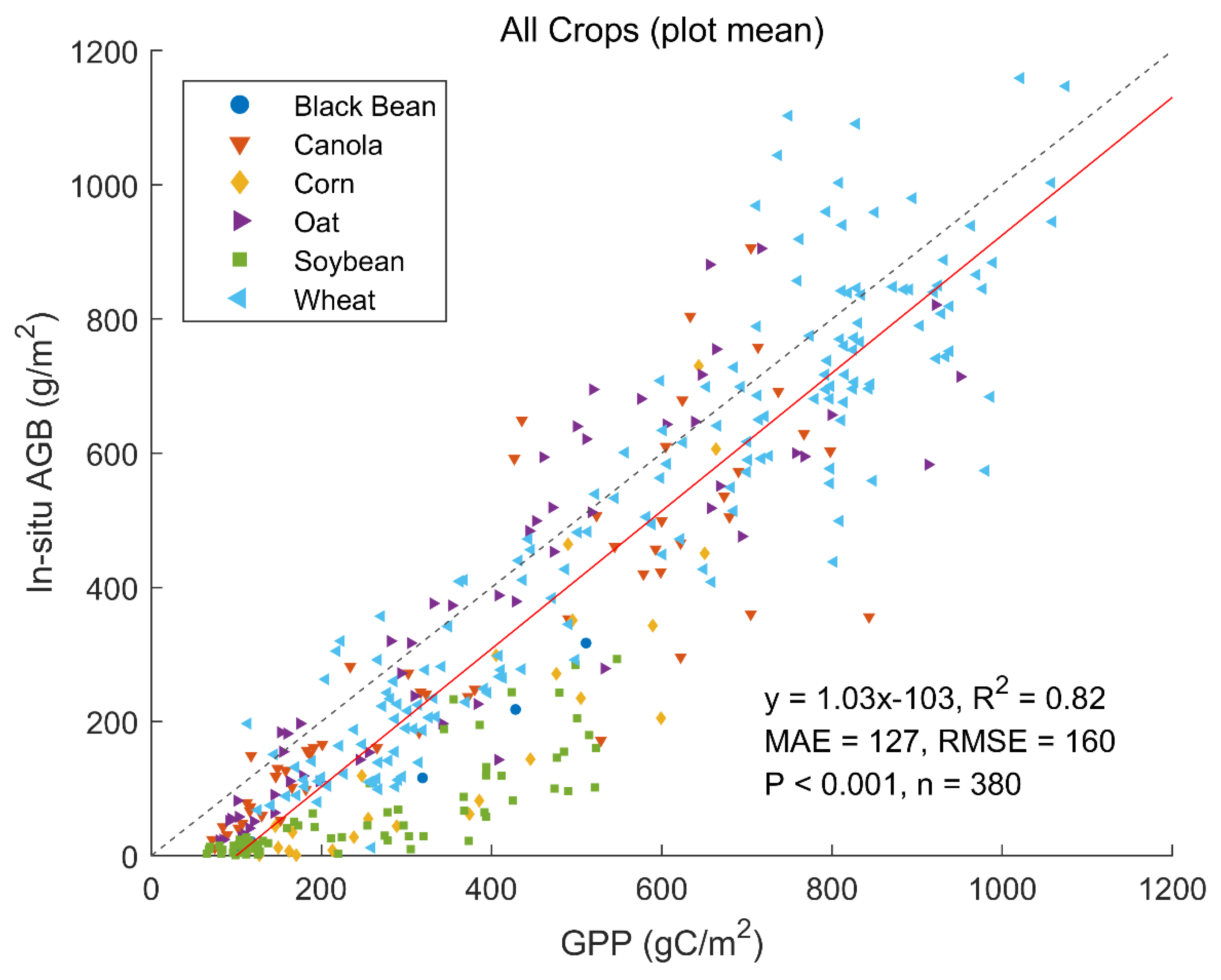
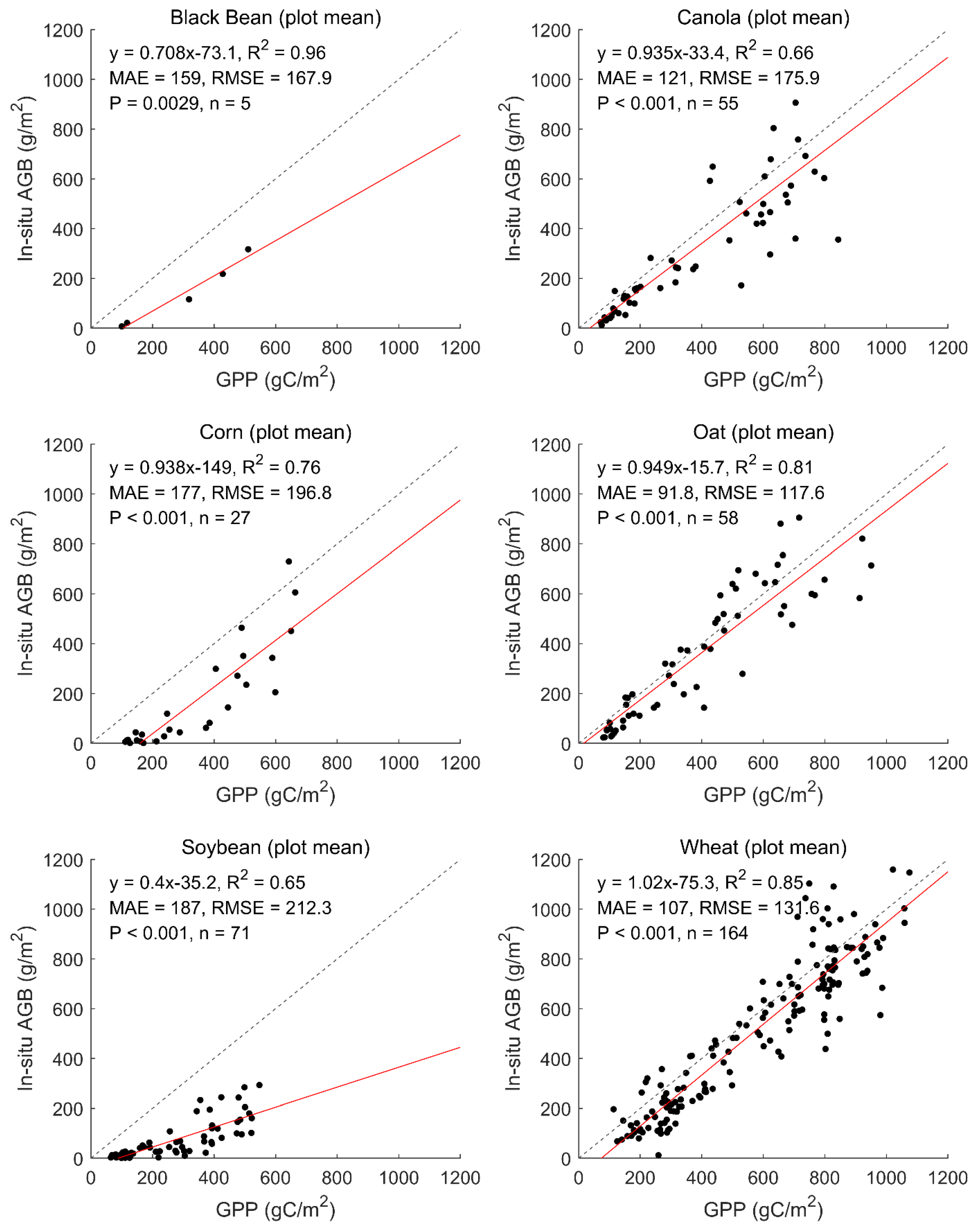
3.1. Correlation between BEPS-Simulated Crop GPP and Ground Measurements

The uncertainty of Sentinel-2-derived LAI time-series after smoothing by LACC from our study has a Root Mean Square Error (RMSE) of 1.1 m² m⁻² (R² = 0.83) compared with the ground-measured plant area index (including crop stems and heads) collected during the SMAPVEX16-MB campaign [67]. A previous validation for the same LAI algorithm reported an RMSE of 0.81 m² m⁻² [68]. Knowledge of the starting and ending dates of the growing season, for each field, is important when simulating crop GPP; this information is clear from the LAI time series. Since the crops in different fields were sowed or planted on different dates, we simply run BEPS from the beginning of 2016. To avoid a numerical problem in the modeling, we have set the minimum LAI to 0.01; these two settings result in an intercept in the GPP–biomass relationships as shown in Figure 3 for all the crop types and in Figure 4, by crop type.

The quality of the LAI time series is important for accurate estimation of AGB. As shown in Figure S2 and Table 1, two Sentinel-2 images are missing in August during key growth periods. This gap leads to inadequate inputs to the LACC method and subsequently, the failure of LAI time-series smoothing, i.e., extreme values in the peak growing season, as observed for the fields in the lower-right corner of our study area. The errors in LAI can propagate into the biomass estimation as indicated by the red circle in Figure S3 and have led to some overestimations in biomass estimation. Although an overall strong correlation between simulated GPP and AGB is observed, these errors highlight the limitation of using Sentinel-2 data alone for biomass mapping. Fusion of Sentinel-2 data with other optical and/or SAR images is one strategy to improve the success of biomass mapping [69].

After excluding the sites with large biases in LAI, Figure 3 shows that the correlation between BEPS-simulated GPP and ground-measured AGB is stronger with R² of 0.82. As the comparison is conducted at a pixel size of 20 m while the AGB is sampled in a lesser area, the AGB samples may not capture all the variations in crop growth present within a 20 m pixel.

Although the V_cmax is likely to vary within the study area, it is set as a constant value. Figure 3 indicates that a unique GPP–biomass relationship is still practical for regional applications.

The slope of 1.03 for the linear relationship between BEPS-simulated GPP and ground-measured AGB, as shown in Figure 3, is reasonable. The slope between GPP and total biomass in high latitudes should be larger than 1.0; however, GPP and only AGB are compared here. The fraction of AGB to total biomass is less than 1, e.g., 78% for maize [70]. Therefore, the CUE (larger than 1) compensates the AGB-to-total-biomass ratio (less than 1), leading to the slope between GPP and AGB close to 1.

The coefficient of determination (R²) between the simulated GPP and AGB ranges from 0.65 to 0.96 for the six crop types (Figure 4). It is worth noting that the two legume crops, black bean and soybean, are characterized with smaller slopes of 0.71 and 0.4, respectively. Legume-cereals have a strong N rhizodeposition and are often cultivated in rotation cropping to enhance crop yield [71]. The N rhizodeposition is associated with large amounts of C rhizodeposition accompanying the senescence of roots and nodules which are made of C [72]. Therefore, a significant amount of biomass is allocated to the below-ground biomass for these crops, leading to a smaller ratio of AGB to total GPP. Qiao et al. [73] found that soybean has greater C rhizodeposition than maize, and the amount of C rhizodeposition varies greatly with soil fertility and organic amendment, presenting a challenge in using GPP for biomass mapping by BEPS or other crop growth models.

Although non-linearity is shown between GPP and AGB of corn, correlation is still high (R² = 0.76) (Figure 4). This suggests that C3 models may be used to simulate GPP of C4 plants if some parameters are adjusted accordingly, although this is subject to further investigation. The correlations between LAI and crop AGB are shown in Figures S4 and S5. For all crop types, crop LAI explains only 50% of variation in crop AGB, significantly lower than that explained by crop GPP (Figure S4); this is because LAI only explains mostly the top part of total AGB; as crop structure varies, the non-leaf part the AGB has a significant difference; for example, corn has far more non-green AGB than the soybean does. This suggests that the cumulative GPP correlates better to AGB which is also a cumulative variable, than it does to the green LAI, which indicates the status of the crop. By crop type, the LAI variations of canola, oat, and wheat explain only 61%, 59%, and 0% of variations in their corresponding AGB, respectively. The LAI variations of black bean, corn, and soybean explain 94%, 81%, and 62% of the variations in their AGB, respectively, higher than that of canola, oat and wheat. This difference can be explained by the growing stages: unlike canola, oat, and wheat, the AGB of black bean, corn and soybean cover only the vegetative growth stage of crop phenology. This is evidenced by the stronger correlation between leaf biomass and LAI (R² = 0.55) than between AGB and LAI (R² = 0.32%) as shown in Figures S6 and S7. Ideally, the LAI should be highly correlated with leaf biomass. However, LAI values derived from Sentinel-2 are equivalent “green” LAIs, resulting from the accumulation leaf pigments and leaf senescence [74]. Therefore, satellite-derived LAI correlates more with green biomass including green stems and fruits [75] and the R² of 0.55 is still considered to be high.

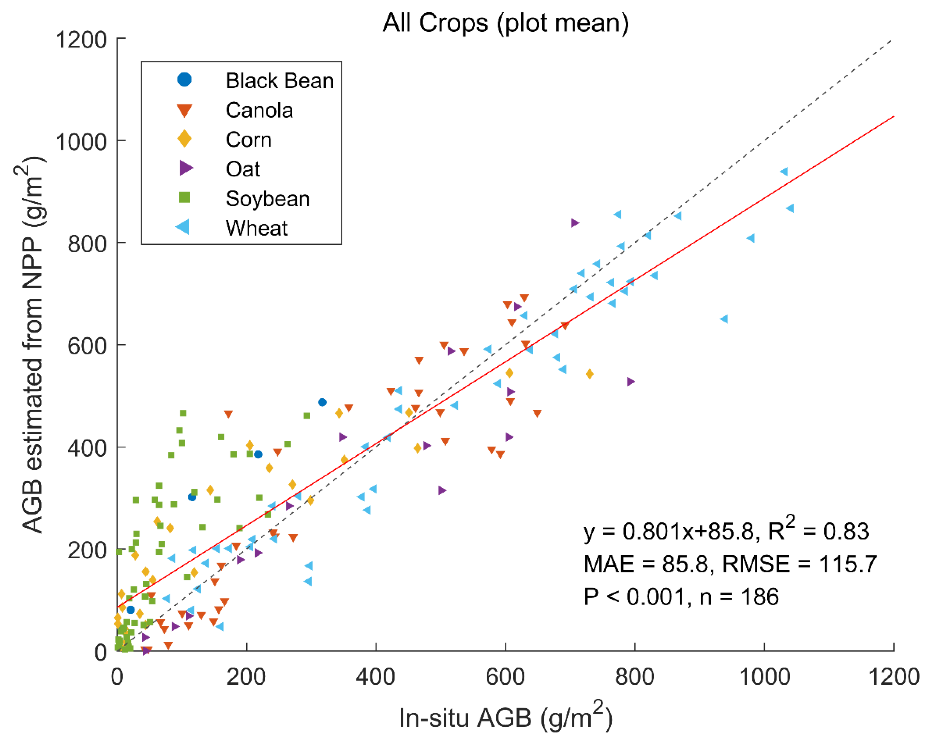
3.2. Correlation between BEPS-Simulated Crop NPP and Ground Measurements

The R² between the simulated NPP and AGB for all the plots is 0.83 (Figure 5); individual R² ranges from 0.56 to 0.95 for the six crop types (Figure 6). There are minor improvements in R² compared to GPP-derived AGB, except for black bean for which the R² is already very high, and for soybean. Similar to GPP-derived AGB, a non-linearity between simulation and measurements is still observed for corn. Since we used the same biomass respiration rates for different crops in BEPS simulations, the minor differences between GPP-derived and NPP-derived AGB are expected. Overall, the RMSE and mean absolute error (MAE) for AGB estimation from NPP are 115.7 and 85.8 g m⁻², respectively.

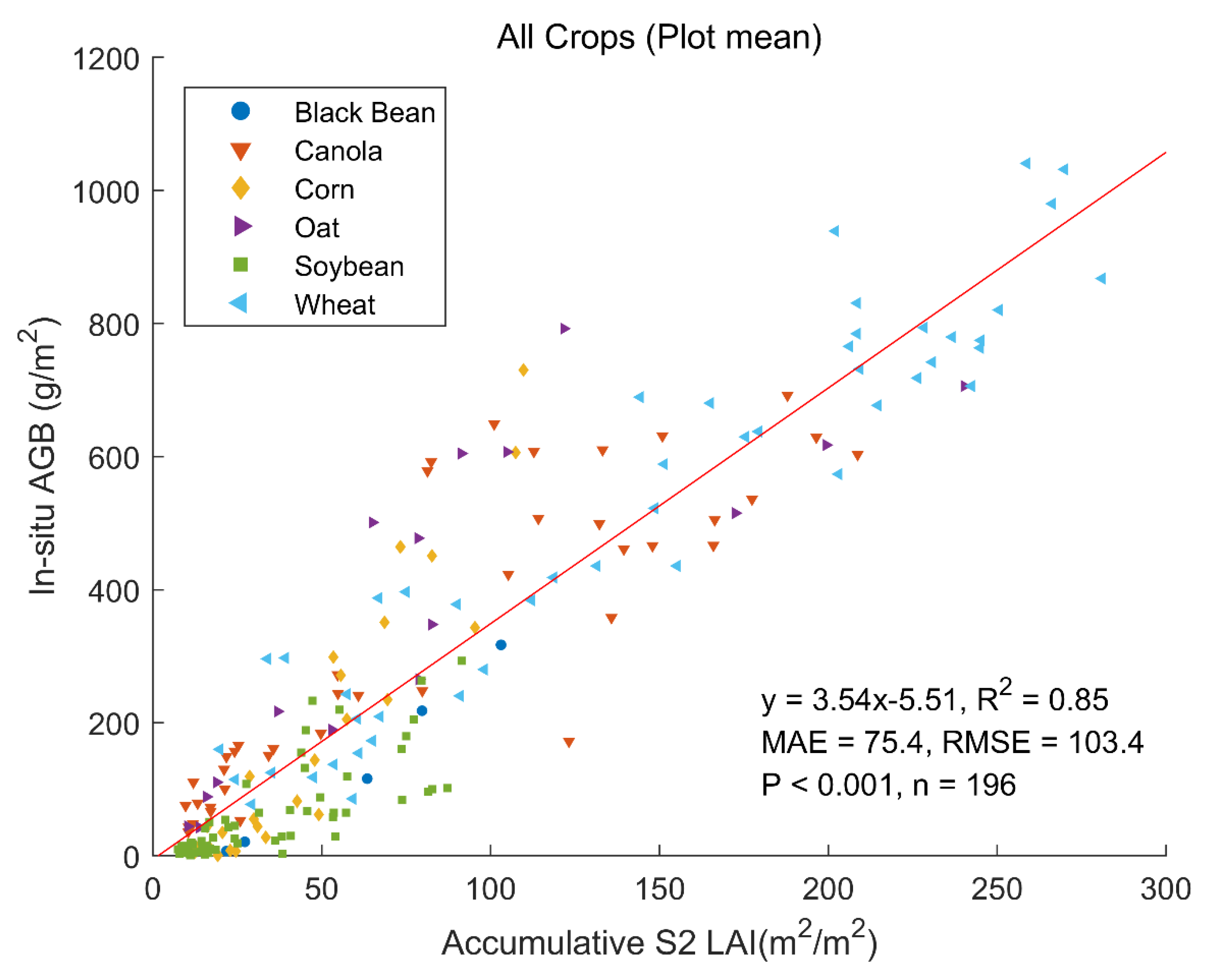
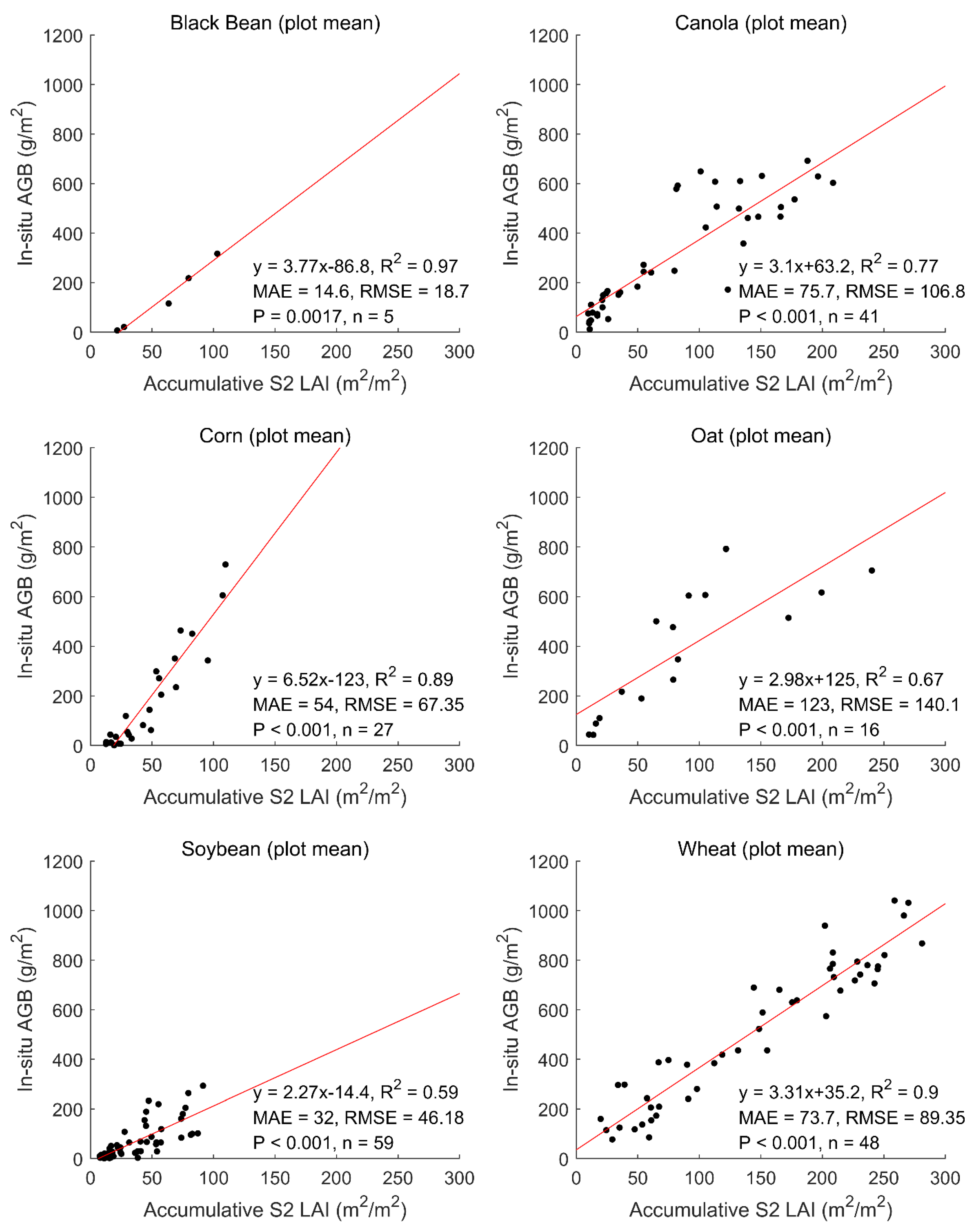
3.3. Correlation between Accumulated LAI and Ground Measurements

The R² between the accumulated S2 LAI and AGB for all the plots is 0.85, which is similar to GPP (R² = 0.82) and NPP (R² = 0.83) (Figure 7); individual R² ranges from 0.59 to 0.97 for the six crop types (Figure 8) with decreased R² for soybean, oat and canola. Notably, the nonlinearity between corn GPP or NPP and AGB is not observed in Figure 8 but the opposite is observed for oat.

Although AGB may be estimated at a similar accuracy by using accumulated S2 LAI for a specific crop type, we believe that GPP- and/or NPP-based approaches produced a reliable overall result for the whole study area. Here, BEPS performs on par with accumulated LAI in biomass estimation because: (1) the accumulated LAI already contains adequate seasonal information for biomass estimation; (2) the meteorological variables do not change much since the study area is small; and (3) certain management information (irrigation, fertilizer use, crop-specific parameters) is unavailable to BEPS. If the study area is big enough to cover different climate zones, we could expect that the BEPS-based estimates will explain more variation in AGB than the accumulated LAI.

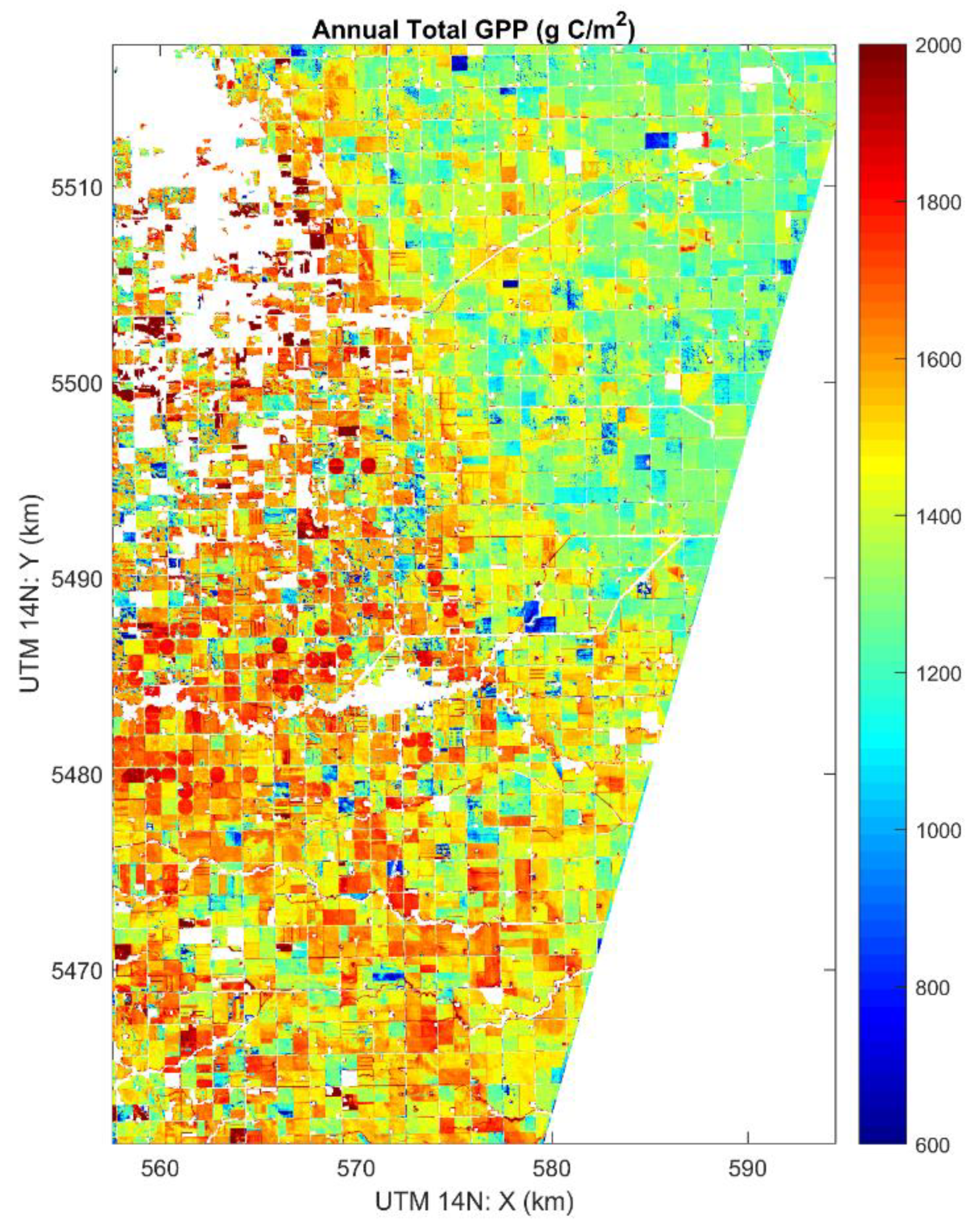
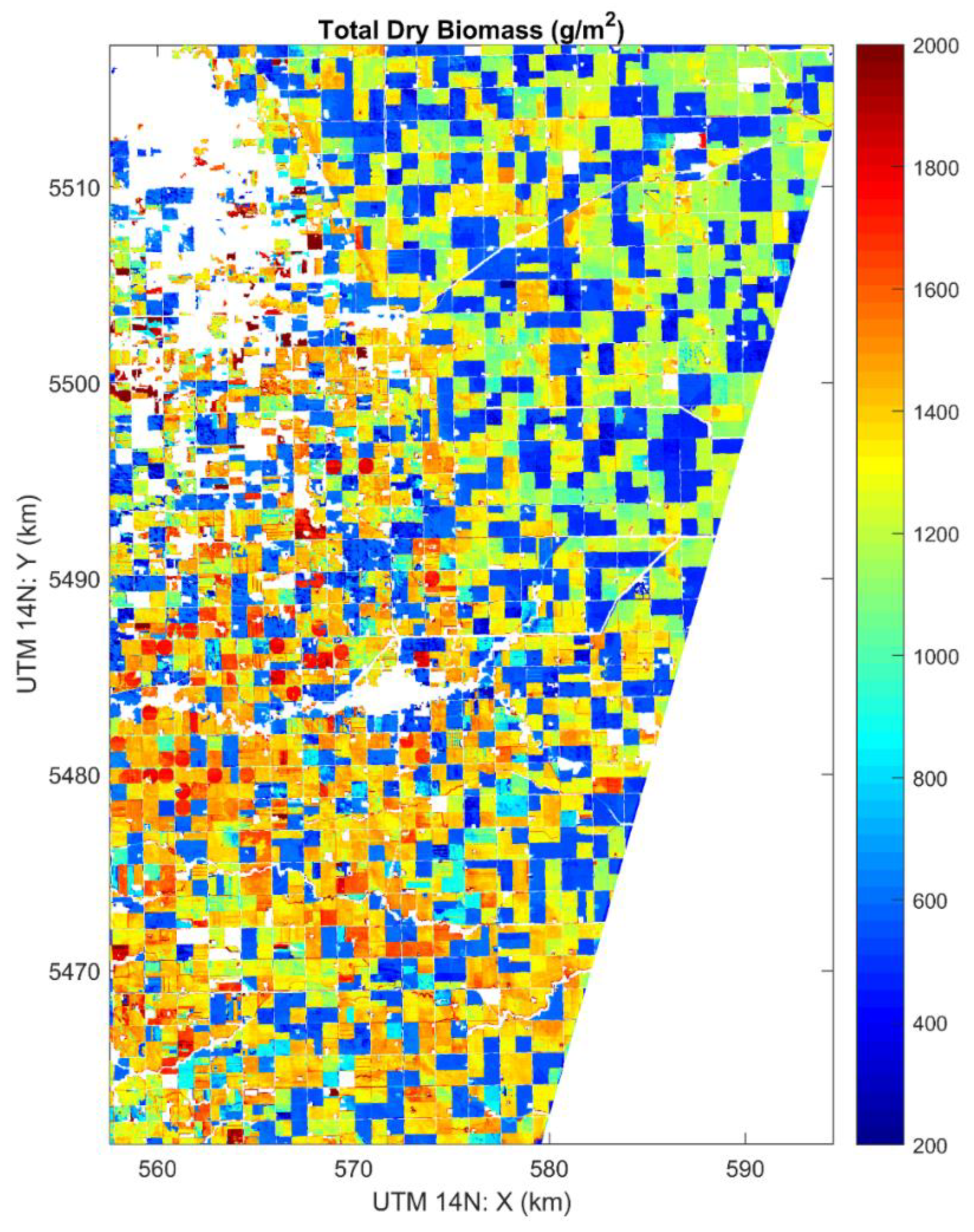
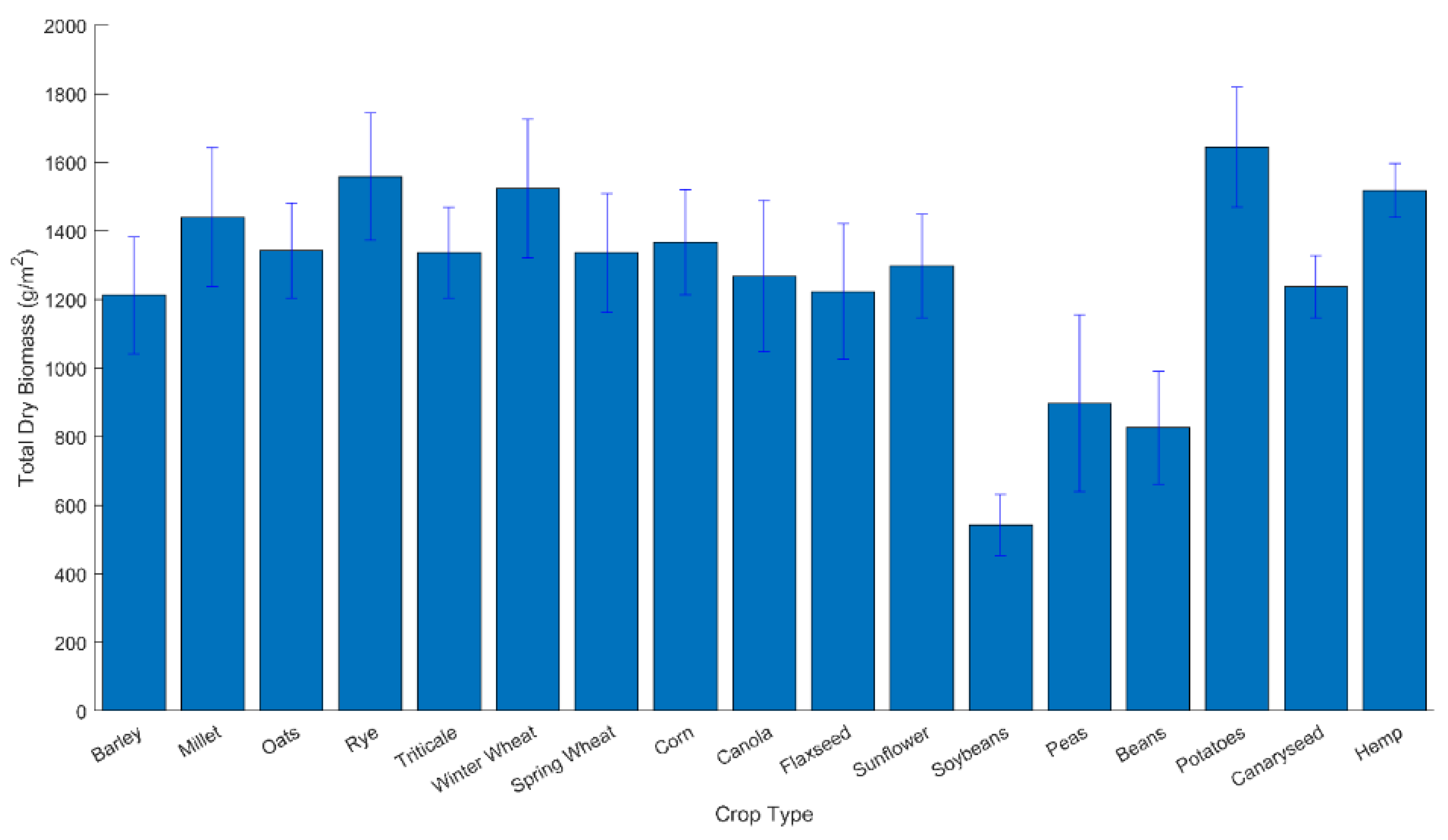
3.4. Spatial Distribution of BEPS-Simulated Crop GPP and AGB

BEPS-simulated GPP for the whole growing season is shown in Figure 9. The lower-right corner is excluded from analysis due to biases in LAI retrievals. In the study area, the crop’s total GPP in the whole growing season ranges from 600 to 2000 g C m⁻² yr⁻¹. Lower GPP values in the upper-right corner are associated with a region of heavy clay soil; for this clay area, the matric water potential can be very low even when the soil water content is relatively high, limiting available water to the crops (Figure S1). The area with center-pivot irrigation (circles; potatoes according to Figure 1) is characterized with high GPP values up to 2000 g C m⁻² yr⁻¹. The variation of GPP is generally small within each field, while considerably larger among different fields, reflecting individual farmer’s management on irrigation and fertilizer use.

The regressions in Figure 3 and Figure 4 are used to derive an AGB map for the study area (Figure 10). For the six target crops, their explicit GPP–AGB relationships are applied; for the rest of crop types, the regression coefficients averaged for all crop types in Figure 3 are applied. In Figure 10, distinct variations among fields are revealed. In the study, the total AGB ranges from 200 to 2000 g m⁻². The peas and beans are characterized with low AGB values (blue area), e.g., 5.4 tons ha⁻¹ for soybean (Figure 11 and Table S1), while potato field has the largest AGB (16.6 tons ha⁻¹). Compared to Figure 9, more variations among fields are observed since the crop-specific calibration from Figure 4 is applied. This suggests that although the accumulative GPP correlates well to the observed AGB, early crop identification/inventory within the crop growing season is critically important for crop growth monitoring and yield prediction.

3.5. Challenges in Using Sentinel-2 Data for Crop Biomass Mapping

Crop identification/classification, crop growth monitoring and crop yield estimation/prediction are among the most important remote sensing applications in agriculture, and they are tightly linked. Crop identification from satellite data provides the basis for annual crop inventory; while crop inventory provides the first order information for yield prediction; a crop classification map is also an important input to the ecosystem model, where the crop-specific parameters can be assigned. Crop growth monitoring from remote sensing involves mapping time-series of crop biophysical parameters (LAI, height, clumping, etc.) and biochemical parameters (e.g., leaf chlorophyll content, Vcmax); a biophysical parameter, AGB, can also be mapped from SAR images at a certain accuracy; the ecosystem model (or some crop growth models) can integrate these remote sensed information, meteorological data, and some available management information to produce reliable GPP, NPP and biomass. Crop biomass, along with crop-specific HI, can then provide more information for yield prediction/estimation than the crop inventory can. In this study, we tested BEPS for biomass mapping using Sentinel-2-derived LAI time-series as main input and with an existing archive of crop inventory map from AAFC.

Although crop AGB is robustly estimated for the majority of our study area, there are a few challenges in applying the same methodology to larger regions at continental and global scales. The same challenges may also apply to general crop growth models with explicit modules of crop phenology development and carbon allocations.

The first challenge is to acquire consistent LAI time-series that are free of cloud contamination. In our study area, there is a one-month gap in August without cloud-free Sentinel-2 images. Although temporal smoothing can mitigate the impact of these gaps to some extent, missing LAI estimates for cloud-contaminated pixels leads to incorrect AGB estimation. It is also a challenge to produce smoothing of LAI time series for near real-time AGB estimation, given the knowledge needed of crop growth stage. To track crop phenology for reliable estimation of AGB, one solution would be to fuse multi-satellite data at similar spatial resolutions, such as from Landsat 7 and 8 optical data and/or Synthetic Aperture Radar data from Sentinel-1 [76].

The second challenge is to perform rigorous model calibration for different crop types, especially for carbon allocations of crops for different cultivars and species, as plants develop different acclimation processes to maximize their photosynthetic capacity. For example, the AGB to GPP ratios range from 0.4 to 1.02 for the six target crops. This is especially true for legume crops with root rhizodeposition. Though not tested in our study, tuber crops such as potatoes can account for a significant amount of underground carbon, and their AGB might have been overestimated in our study. The accuracy of using C3 model to simulate AGB of C4 plant (corn in this study) is acceptable but not optimal.

The third challenge is to acquire soil nutrition conditions of the field and relate this information to photosynthetic capacity of crops. Although some crop growth models have a mechanism to relate nitrogen pool of crop system to leaf V_cmax, such nitrogen management information is unavailable at the regional and national scales. Although Sentinel-2 has the red-edge bands for retrieval of leaf chlorophyll content [77,78,79,80], how leaf chlorophyll content correlates with leaf V_cmax among species, crop growth stages and radiation conditions are not completely understood.

The fourth challenge is to acquire pixel-level irrigation information for crop growth models. Without correct irrigation information as an input, crop GPP and NPP may be underestimated by the models [46]. Sentinel-1 C-band SAR may be used for soil moisture mapping but only when the canopy is sparse [81]. The SMAP L-band radiometer has superior sensitivity to surface soil moisture even at moderate canopy water content, but its spatial resolution is low (40 km) [82]. Although some studies have integrated SAR data at high resolution and with SMAP radiometer data to produce soil moisture at a 1 km resolution [83], it is still impractical to do this at the 20 m resolution.

The last challenge for crop biomass mapping using models is the limitation of computation resources. For example, it takes half a day to simulate crop GPP at a 20 m resolution using a 54-core computer (2.5 Ghz) for our study area. This means that, for these process-based deterministic models, the computation of GPP mapping for a county at 20 m resolution is comparable to the GPP simulation of a global ecosystem at the 0.1° resolution. If a data assimilation approach, such as the ensemble Kalman filter (EnKF) is used to assimilate any crop biophysical parameter into a crop growth model, the computation will be increased by an order of 1 to 2, suggesting that it is almost impossible to make use of EnKF for data assimilation at the current cost of computation.

These challenges, although not limited to Sentinel-2 data applications, suggest that although BEPS (hourly version) has an advanced model structure to simulate canopy-scale photosynthesis [52], this requires significant computation effort. In contrast, some crop growth models are executed at a daily step and/or LUE-based photosynthesis model [15,20,21], but with the strength of crop traits modeling and handling of soil nutrition and water management. However, such an approach necessitates availability of these crop traits at large scales. Operational crop biomass (and yield) mapping may require a compromise between large scale and high spatial, and simplicity of the model structure. Mapping biomass at field scales (segmentation from crop identification map) might be a good alternative approach to address current big-data challenges.

Similar to this work, two recent studies have used Sentinel-2-derived LAI for biomass and yield mapping. Punalekar et al. [84] reported that the R² between pasture biomass and LAI ranges from 0.16–0.73 to 0.22–0.76, for the NDVI-derived LAI and radiative transfer model-based LAI, respectively. Lambert, Traoré, Blaes, Baret and Defourny [30] demonstrated that the R² values between LAI and yield are 0.68, 0.62, 0.8 and 0.48 for cotton, maize, millet and sorghum, respectively. Here, we show that the R² values between GPP and AGB range from 0.65 to 0.96 for six annual crops which dominate Manitoba’s agro-ecosystem. Despite these aforementioned challenges, our study demonstrates the advantage of using LAI time-series and integrating both biotic and abiotic factors for biomass mapping at very high spatial resolutions.

4. Conclusions

This research explores the potential of integrating high spatio-temporal leaf area index (LAI) estimates derived from Sentinel-2 spectral reflectance data with an ecosystem model for crop above-ground biomass (AGB) mapping at the regional scale. The accuracy of this approach is evaluated using crop AGB field data collected during the SMAPVEX16-MB experiment conducted in western Canada, in 2016. Considering abiotic factors derived from meteorological data and soils data and LAI from Sentinel-2, we find that the model-simulated crop gross primary production (GPP) at a 20 m resolution explains 82% of the variation in the annual crop AGB for six annual crop types. The results outperform the biomass mapping using LAI alone. The correlation between the model-simulated GPP and ground measured AGB for each of the six crop types is also strong, suggesting that our approach is reliable for AGB mapping at a high spatial resolution. Similarly, crop NPP and accumulative LAI explain 83% and 85% of the variation in the crop AGB, suggesting the importance of using temporal information from remote sensing.

The challenges for crop AGB mapping at high resolution are also discussed. These include difficulty in acquiring temporally consistent LAI time series due to cloud contamination, the lack of soil nutrition and water management information, the need for model calibration at the regional and national scales, and the high cost of computation. A practical approach for crop biomass mapping should include a compromise among data accessibility, model complexity, and computational resource availability.

References

1. Ahamed, T.; Tian, L.; Zhang, Y.; Ting, K.C. A review of remote sensing methods for biomass feedstock production. Biomass Bioenergy 2011, 35, 2455–2469. [Google Scholar] [CrossRef]
2. Chao, Z.; Liu, N.; Zhang, P.; Ying, T.; Song, K. Estimation methods developing with remote sensing information for energy crop biomass: A comparative review. Biomass Bioenergy 2019, 122, 414–425. [Google Scholar] [CrossRef]
3. Fu, Y.; Yang, G.; Wang, J.; Song, X.; Feng, H. Winter wheat biomass estimation based on spectral indices, band depth analysis and partial least squares regression using hyperspectral measurements. Comput. Electron. Agric. 2014, 100, 51–59. [Google Scholar] [CrossRef]
4. Ren, H.; Zhou, G. Estimating senesced biomass of desert steppe in Inner Mongolia using field spectrometric data. Agric. For. Meteorol. 2012, 161, 66–71. [Google Scholar] [CrossRef]
5. Prabhakara, K.; Hively, W.D.; McCarty, G.W. Evaluating the relationship between biomass, percent groundcover and remote sensing indices across six winter cover crop fields in Maryland, United States. Int. J. Appl. Earth Obs. Geoinf. 2015, 39, 88–102. [Google Scholar] [CrossRef] [Green Version]
6. Han, J.; Wei, C.; Chen, Y.; Liu, W.; Song, P.; Zhang, D.; Wang, A.; Song, X.; Wang, X.; Huang, J. Mapping above-ground biomass of winter oilseed rape using high spatial resolution satellite data at parcel scale under waterlogging conditions. Remote Sens. 2017, 9, 238. [Google Scholar] [CrossRef] [Green Version]
7. Yue, J.; Yang, G.; Tian, Q.; Feng, H.; Xu, K.; Zhou, C. Estimate of winter-wheat above-ground biomass based on UAV ultrahigh-ground-resolution image textures and vegetation indices. ISPRS J. Photogramm. Remote Sens. 2019, 150, 226–244. [Google Scholar] [CrossRef]
8. Bendig, J.; Bolten, A.; Bennertz, S.; Broscheit, J.; Eichfuss, S.; Bareth, G. Estimating biomass of barley using crop surface models (CSMs) derived from UAV-based RGB imaging. Remote Sens. 2014, 6, 10395–10412. [Google Scholar] [CrossRef] [Green Version]
9. Näsi, R.; Viljanen, N.; Kaivosoja, J.; Alhonoja, K.; Hakala, T.; Markelin, L.; Honkavaara, E. Estimating biomass and nitrogen amount of barley and grass using UAV and aircraft based spectral and photogrammetric 3D features. Remote Sens. 2018, 10, 1082. [Google Scholar] [CrossRef] [Green Version]
10. Maimaitijiang, M.; Sagan, V.; Sidike, P.; Maimaitiyiming, M.; Hartling, S.; Peterson, K.T.; Maw, M.J.W.; Shakoor, N.; Mockler, T.; Fritschi, F.B. Vegetation Index Weighted Canopy Volume Model (CVMVI) for soybean biomass estimation from Unmanned Aerial System-based RGB imagery. ISPRS J. Photogramm. Remote Sens. 2019, 151, 27–41. [Google Scholar] [CrossRef]
11. Ndikumana, E.; Ho Tong Minh, D.; Nguyen Hai Thu, D.; Baghdadi, N.; Courault, D.; Hossard, L.; El Moussawi, I. Rice Height and Biomass Estimations Using Multitemporal SAR Sentinel-1: Camargue Case Study. In Proceedings of the 20th Remote Sensing for Agriculture, Ecosystems, and Hydrology Conference, Berlin, Germany, 10–13 September 2018; The International Society for Optical Engineering (SPIE): Bellingham, WA, USA, 2018. [Google Scholar]
12. Yang, H.; Yang, G.; Gaulton, R.; Zhao, C.; Li, Z.; Taylor, J.; Wicks, D.; Minchella, A.; Chen, E.; Yang, X. In-season biomass estimation of oilseed rape (Brassica napus L.) using fully polarimetric SAR imagery. Precis. Agric. 2019, 20, 630–648. [Google Scholar] [CrossRef] [Green Version]
13. Yang, S.; Feng, Q.; Liang, T.; Liu, B.; Zhang, W.; Xie, H. Modeling grassland above-ground biomass based on artificial neural network and remote sensing in the Three-River Headwaters Region. Remote Sens. Environ. 2018, 204, 448–455. [Google Scholar] [CrossRef]
14. Mandal, D.; Kumar, V.; McNairn, H.; Bhattacharya, A.; Rao, Y.S. Joint estimation of Plant Area Index (PAI) and wet biomass in wheat and soybean from C-band polarimetric SAR data. Int. J. Appl. Earth Obs. Geoinf. 2019, 79, 24–34. [Google Scholar] [CrossRef]
15. Huang, J.; Gómez-Dans, J.L.; Huang, H.; Ma, H.; Wu, Q.; Lewis, P.E.; Liang, S.; Chen, Z.; Xue, J.-H.; Wu, Y.; et al. Assimilation of remote sensing into crop growth models: Current status and perspectives. Agric. For. Meteorol. 2019, 276–277, 107609. [Google Scholar] [CrossRef]
16. Liao, C.; Wang, J.; Dong, T.; Shang, J.; Liu, J.; Song, Y. Using spatio-temporal fusion of Landsat-8 and MODIS data to derive phenology, biomass and yield estimates for corn and soybean. Sci. Total Environ. 2019, 650, 1707–1721. [Google Scholar] [CrossRef]
17. Battude, M.; Al Bitar, A.; Morin, D.; Cros, J.; Huc, M.; Sicre, C.M.; Le Dantec, V.; Demarez, V. Estimating maize biomass and yield over large areas using high spatial and temporal resolution Sentinel-2 like remote sensing data. Remote Sens. Environ. 2016, 184, 668–681. [Google Scholar] [CrossRef]
18. Campos, I.; González-Gómez, L.; Villodre, J.; González-Piqueras, J.; Suyker, A.E.; Calera, A. Remote sensing-based crop biomass with water or light-driven crop growth models in wheat commercial fields. Field Crop. Res. 2018, 216, 175–188. [Google Scholar] [CrossRef]
19. Dong, T.; Liu, J.; Qian, B.; He, L.; Liu, J.; Wang, R.; Jing, Q.; Champagne, C.; McNairn, H.; Powers, J.; et al. Estimating crop biomass using leaf area index derived from Landsat 8 and Sentinel-2 data. ISPRS J. Photogramm. Remote Sens. 2020, 168, 236–250. [Google Scholar] [CrossRef]
20. Jones, J.W.; Hoogenboom, G.; Porter, C.H.; Boote, K.J.; Batchelor, W.D.; Hunt, L.A.; Wilkens, P.W.; Singh, U.; Gijsman, A.J.; Ritchie, J.T. The DSSAT cropping system model. Eur. J. Agron. 2003, 18, 235–265. [Google Scholar] [CrossRef]
21. Williams, J.R.; Jones, C.A.; Kiniry, J.R.; Spanel, D.A. EPIC crop growth model. Trans. Am. Soc. Agric. Eng. 1989, 32, 497–511. [Google Scholar] [CrossRef]
22. Khan, A.; Stöckle, C.O.; Nelson, R.L.; Peters, T.; Adam, J.C.; Lamb, B.; Chi, J.; Waldo, S. Estimating biomass and yield using metric evapotranspiration and simple growth algorithms. Agron. J. 2019, 111, 536–544. [Google Scholar] [CrossRef] [Green Version]
23. Schlesinger, W.H. Biogeochemistry: An Analysis of Global Change; Academic Press: San Diego, CA, USA, 1991. [Google Scholar]
24. Machwitz, M.; Giustarini, L.; Bossung, C.; Frantz, D.; Schlerf, M.; Lilienthal, H.; Wandera, L.; Matgen, P.; Hoffmann, L.; Udelhoven, T. Enhanced biomass prediction by assimilating satellite data into a crop growth model. Environ. Model. Softw. 2014, 62, 437–453. [Google Scholar] [CrossRef]
25. Novelli, F.; Spiegel, H.; Sandén, T.; Vuolo, F. Assimilation of Sentinel-2 Leaf Area Index Data into a Physically-Based Crop Growth Model for Yield Estimation. Agronomy 2019, 9, 255. [Google Scholar] [CrossRef] [Green Version]
26. Dong, T.; Liu, J.; Qian, B.; Zhao, T.; Jing, Q.; Geng, X.; Wang, J.; Huffman, T.; Shang, J. Estimating winter wheat biomass by assimilating leaf area index derived from fusion of Landsat-8 and MODIS data. Int. J. Appl. Earth Obs. Geoinf. 2016, 49, 63–74. [Google Scholar] [CrossRef]
27. Lokupitiya, E.; Lefsky, M.; Paustian, K. Use of AVHRR NDVI time series and ground-based surveys for estimating county-level crop biomass. Int. J. Remote Sens. 2010, 31, 141–158. [Google Scholar] [CrossRef]
28. Perry, E.M.; Morse-Mcnabb, E.M.; Nuttall, J.G.; O’Leary, G.J.; Clark, R. Managing wheat from space: Linking MODIS NDVI and crop models for predicting australian dryland wheat biomass. IEEE J. Sel. Top. Appl. Earth Obs. Remote Sens. 2014, 7, 3724–3731. [Google Scholar] [CrossRef]
29. Yan, F.; Wu, B.; Wang, Y. Estimating aboveground biomass in Mu Us Sandy Land using Landsat spectral derived vegetation indices over the past 30 years. J. Arid Land 2013, 5, 521–530. [Google Scholar] [CrossRef] [Green Version]
30. Lambert, M.J.; Traoré, P.C.S.; Blaes, X.; Baret, P.; Defourny, P. Estimating smallholder crops production at village level from Sentinel-2 time series in Mali’s cotton belt. Remote Sens. Environ. 2018, 216, 647–657. [Google Scholar] [CrossRef]
31. Kross, A.; McNairn, H.; Lapen, D.; Sunohara, M.; Champagne, C. Assessment of RapidEye vegetation indices for estimation of leaf area index and biomass in corn and soybean crops. Int. J. Appl. Earth Obs. Geoinf. 2015, 34, 235–248. [Google Scholar] [CrossRef] [Green Version]
32. Wolanin, A.; Camps-Valls, G.; Gómez-Chova, L.; Mateo-García, G.; Van der Tol, C.; Zhang, Y.; Guanter, L. Estimating crop primary productivity with Sentinel-2 and Landsat 8 using machine learning methods trained with radiative transfer simulations. Remote Sens. Environ. 2019, 225, 441–457. [Google Scholar] [CrossRef]
33. Gao, F.; Anderson, M.; Daughtry, C.; Johnson, D. Assessing the Variability of Corn and Soybean Yields in Central Iowa Using High Spatiotemporal Resolution Multi-Satellite Imagery. Remote Sens. 2018, 10, 1489. [Google Scholar] [CrossRef] [Green Version]
34. Habyarimana, E.; Piccard, I.; Catellani, M.; De Franceschi, P.; Dall’Agata, M. Towards Predictive Modeling of Sorghum Biomass Yields Using Fraction of Absorbed Photosynthetically Active Radiation Derived from Sentinel-2 Satellite Imagery and Supervised Machine Learning Techniques. Agronomy 2019, 9, 203. [Google Scholar] [CrossRef] [Green Version]
35. Sibanda, M.; Mutanga, O.; Rouget, M. Examining the potential of Sentinel-2 MSI spectral resolution in quantifying above ground biomass across different fertilizer treatments. ISPRS J. Photogramm. Remote Sens. 2015, 110, 55–65. [Google Scholar] [CrossRef]
36. Jin, Z.; Azzari, G.; You, C.; Di Tommaso, S.; Aston, S.; Burke, M.; Lobell, D.B. Smallholder maize area and yield mapping at national scales with Google Earth Engine. Remote Sens. Environ. 2019, 228, 115–128. [Google Scholar] [CrossRef]
37. Liu, J.; Chen, J.M.; Cihlar, J.; Park, W.M. A process-based boreal ecosystem productivity simulator using remote sensing inputs. Remote Sens. Environ. 1997, 62, 158–175. [Google Scholar] [CrossRef]
38. Chen, J.M.; Liu, J.; Cihlar, J.; Goulden, M.L. Daily canopy photosynthesis model through temporal and spatial scaling for remote sensing applications. Ecol. Model. 1999, 124, 99–119. [Google Scholar] [CrossRef] [Green Version]
39. Ju, W.; Chen, J.M.; Black, T.A.; Barr, A.G.; Liu, J.; Chen, B. Modelling multi-year coupled carbon and water fluxes in a boreal aspen forest. Agric. For. Meteorol. 2006, 140, 136–151. [Google Scholar] [CrossRef]
40. Chen, B.; Chen, J.M.; Ju, W. Remote sensing-based ecosystem–atmosphere simulation scheme (EASS)—Model formulation and test with multiple-year data. Ecol. Model. 2007, 209, 277–300. [Google Scholar] [CrossRef]
41. He, L.; Chen, J.M.; Liu, J.; Mo, G.; Bélair, S.; Zheng, T.; Wang, R.; Chen, B.; Croft, H.; Arain, M.A.; et al. Optimization of water uptake and photosynthetic parameters in an ecosystem model using tower flux data. Ecol. Model. 2014, 294, 94–104. [Google Scholar] [CrossRef]
42. Matsushita, B.; Xu, M.; Chen, J.; Kameyama, S.; Tamura, M. Estimation of regional net primary productivity (NPP) using a process-based ecosystem model: How important is the accuracy of climate data? Ecol. Model. 2004, 178, 371–388. [Google Scholar] [CrossRef]
43. Feng, X.; Liu, G.; Chen, J.M.; Chen, M.; Liu, J.; Ju, W.M.; Sun, R.; Zhou, W. Net primary productivity of China’s terrestrial ecosystems from a process model driven by remote sensing. J. Environ. Manag. 2007, 85, 563–573. [Google Scholar] [CrossRef] [PubMed]
44. Chen, J.M.; Mo, G.; Pisek, J.; Liu, J.; Deng, F.; Ishizawa, M.; Chan, D. Effects of foliage clumping on the estimation of global terrestrial gross primary productivity. Glob. Biogeochem. Cycles 2012, 26. [Google Scholar] [CrossRef]
45. Luo, X.; Croft, H.; Chen, J.M.; He, L.; Keenan, T.F. Improved estimates of global terrestrial photosynthesis using information on leaf chlorophyll content. Glob. Chang. Biol. 2019, 25, 2499–2514. [Google Scholar] [CrossRef] [Green Version]
46. He, L.; Chen, J.M.; Liu, J.; Bélair, S.; Luo, X. Assessment of SMAP soil moisture for global simulation of gross primary production. J. Geophys. Res. Biogeosci. 2017, 122, 1549–1563. [Google Scholar] [CrossRef]
47. He, L.M.; Chen, J.M.; Gonsamo, A.; Luo, X.Z.; Wang, R.; Liu, Y.; Liu, R.G. Changes in the Shadow: The Shifting Role of Shaded Leaves in Global Carbon and Water Cycles Under Climate Change. Geophys. Res. Lett. 2018, 45, 5052–5061. [Google Scholar] [CrossRef] [Green Version]
48. He, L.; Chen, J.M.; Liu, J.; Zheng, T.; Wang, R.; Joiner, J.; Chou, S.; Chen, B.; Liu, Y.; Liu, R.; et al. Diverse photosynthetic capacity of global ecosystems mapped by satellite chlorophyll fluorescence measurements. Remote Sens. Environ. 2019, 232, 111344. [Google Scholar] [CrossRef] [PubMed]
49. Wang, P.; Sun, R.; Zhang, J.; Zhou, Y.; Xie, D.; Zhu, Q. Yield estimation of winter wheat in the North China Plain using the remote-sensing–photosynthesis–yield estimation for crops (RS–P–YEC) model. Int. J. Remote Sens. 2011, 32, 6335–6348. [Google Scholar] [CrossRef]
50. He, L.; Mostovoy, G. Cotton yield estimate using Sentinel-2 data and an ecosystem model over the southern US. Remote Sens. 2019, 11, 2000. [Google Scholar] [CrossRef] [Green Version]
51. Farquhar, G.D.; Caemmerer, S.V.; Berry, J.A. A Biochemical-Model of Photosynthetic Co2 Assimilation in Leaves of C-3 Species. Planta 1980, 149, 78–90. [Google Scholar] [CrossRef] [PubMed] [Green Version]
52. Luo, X.Z.; Chen, J.M.; Liu, J.E.; Black, T.A.; Croft, H.; Staebler, R.; He, L.M.; Arain, M.A.; Chen, B.; Mo, G.; et al. Comparison of Big-Leaf, Two-Big-Leaf, and Two-Leaf Upscaling Schemes for Evapotranspiration Estimation Using Coupled Carbon-Water Modeling. J. Geophys. Res. Biogeosci. 2018, 123, 207–225. [Google Scholar] [CrossRef]
53. Sharwood, R.E.; Sonawane, B.V.; Ghannoum, O. Photosynthetic flexibility in maize exposed to salinity and shade. J. Exp. Bot. 2014, 65, 3715–3724. [Google Scholar] [CrossRef] [Green Version]
54. Zhang, Y.; Xu, M.; Chen, H.; Adams, J. Global pattern of NPP to GPP ratio derived from MODIS data: Effects of ecosystem type, geographical location and climate. Glob. Ecol. Biogeogr. 2009, 18, 280–290. [Google Scholar] [CrossRef]
55. Tang, X.; Carvalhais, N.; Moura, C.; Ahrens, B.; Koirala, S.; Fan, S.; Guan, F.; Zhang, W.; Gao, S.; Magliulo, V.; et al. Global variability of carbon use efficiency in terrestrial ecosystems. Biogeosci. Discuss. 2019, 2019, 1–19. [Google Scholar] [CrossRef] [Green Version]
56. Manzoni, S.; Čapek, P.; Porada, P.; Thurner, M.; Winterdahl, M.; Beer, C.; Brüchert, V.; Frouz, J.; Herrmann, A.M.; Lindahl, B.D.; et al. Reviews and syntheses: Carbon use efficiency from organisms to ecosystems—Definitions, theories, and empirical evidence. Biogeosciences 2018, 15, 5929–5949. [Google Scholar] [CrossRef] [Green Version]
57. He, Y.; Piao, S.; Li, X.; Chen, A.; Qin, D. Global patterns of vegetation carbon use efficiency and their climate drivers deduced from MODIS satellite data and process-based models. Agric. For. Meteorol. 2018, 256–257, 150–158. [Google Scholar] [CrossRef]
58. Bhuiyan, H.A.K.M.; McNairn, H.; Powers, J.; Friesen, M.; Pacheco, A.; Jackson, T.J.; Cosh, M.H.; Colliander, A.; Berg, A.; Rowlandson, T.; et al. Assessing SMAP Soil Moisture Scaling and Retrieval in the Carman (Canada) Study Site. Vadose Zone J. 2018, 17, 180132. [Google Scholar] [CrossRef] [Green Version]
59. McNairn, H.H.; Gottfried, K.; Powers, J. SMAPVEX16 Manitoba Leaf Area Index, Version 1; NASA National Snow and Ice Data Center Distributed Active Archive Center: Boulder, CO, USA, 2018. [Google Scholar] [CrossRef]
60. Richter, R.; Louis, J.; Müller-Wilm, U. Sentinel-2 MSI—Level 2A Products Algorithm Theoretical Basis Document; S2PAD-ATBD-0001; Deutsches Zentrum für Luft- und Raumfahrt e.V. (DLR), VEGA Technologies SAS: Darmstadt, Germany, 2012; p. 87. [Google Scholar]
61. Deng, F.; Chen, J.M.; Plummer, S.; Chen, M.Z.; Pisek, J. Algorithm for global leaf area index retrieval using satellite imagery. IEEE Trans. Geosci. Remote Sens. 2006, 44, 2219–2229. [Google Scholar] [CrossRef] [Green Version]
62. Chen, J.M.; Leblanc, S.G. A four-scale bidirectional reflectance model based on canopy architecture. IEEE Trans. Geosci. Remote Sens. 1997, 35, 1316–1337. [Google Scholar] [CrossRef]
63. Chen, J.M.; Deng, F.; Chen, M.Z. Locally adjusted cubic-spline capping for reconstructing seasonal trajectories of a satellite-derived surface parameter. IEEE Trans. Geosci. Remote Sens. 2006, 44, 2230–2238. [Google Scholar] [CrossRef]
64. Rienecker, M.M.; Suarez, M.J.; Gelaro, R.; Todling, R.; Bacmeister, J.; Liu, E.; Bosilovich, M.G.; Schubert, S.D.; Takacs, L.; Kim, G.K.; et al. MERRA: NASA’s Modern-Era Retrospective Analysis for Research and Applications. J. Clim. 2011, 24, 3624–3648. [Google Scholar] [CrossRef]
65. Hengl, T.; De Jesus, J.M.; Heuvelink, G.B.M.; Gonzalez, M.R.; Kilibarda, M.; Blagotić, A.; Shangguan, W.; Wright, M.N.; Geng, X.; Bauer-Marschallinger, B.; et al. SoilGrids250m: Global gridded soil information based on machine learning. PLoS ONE 2017, 12, e0169748. [Google Scholar] [CrossRef] [Green Version]
66. Fisette, T.; Rollin, P.; Aly, Z.; Campbell, L.; Daneshfar, B.; Filyer, P.; Smith, A.; Davidson, A.; Shang, J.; Jarvis, I. AAFC Annual Crop Inventory: Status and Challenges. In Proceedings of the 2nd International Conference on Agro-Geoinformatics: Information for Sustainable Agriculture, Agro-Geoinformatics, Fairfax, VA, USA, 12–16 August 2013; pp. 270–274. [Google Scholar]
67. Wang, R.; Chen, J.M.; He, L.; Liu, J.; Shang, J.; Liu, J.; Dong, T. A novel semi-empirical model for crop leaf area index retrieval using RADARSAT-2 co- and cross-polarizations. ISPRS J. Photogramm. Remote Sens. 2020. summitted. [Google Scholar]
68. Liu, Y.; Liu, R.G.; Chen, J.M. Retrospective retrieval of long-term consistent global leaf area index (1981–2011) from combined AVHRR and MODIS data. J. Geophys. Res. Biogeosci. 2012, 117, 117. [Google Scholar] [CrossRef]
69. Gao, F.; Morisette, J.T.; Wolfe, R.E.; Ederer, G.; Pedelty, J.; Masuoka, E.; Myneni, R.; Tan, B.; Nightingale, J. An Algorithm to Produce Temporally and Spatially Continuous MODIS-LAI Time Series. IEEE Geosci. Remote Sens. Lett. 2008, 5, 60–64. [Google Scholar] [CrossRef]
70. Amos, B.; Walters, D.T. Maize Root Biomass and Net Rhizodeposited Carbon. Soil Sci. Soc. Am. J. 2006, 70, 1489–1503. [Google Scholar] [CrossRef]
71. Zang, H.; Yang, X.; Feng, X.; Qian, X.; Hu, Y.; Ren, C.; Zeng, Z. Rhizodeposition of nitrogen and carbon by mungbean (Vigna radiata L.) and its contribution to intercropped oats (Avena nuda L.). PLoS ONE 2015, 10, e0121132. [Google Scholar] [CrossRef]
72. Fustec, J.; Lesuffleur, F.; Mahieu, S.; Cliquet, J.-B. Nitrogen rhizodeposition of legumes. A review. Agron. Sustain. Dev. 2010, 30, 57–66. [Google Scholar] [CrossRef] [Green Version]
73. Qiao, Y.; Miao, S.; Han, X.; Yue, S.; Tang, C. Improving soil nutrient availability increases carbon rhizodeposition under maize and soybean in Mollisols. Sci. Total Environ. 2017, 603–604, 416–424. [Google Scholar] [CrossRef] [PubMed]
74. Wang, R.; Chen, J.M.; Liu, Z.; Arain, A. Evaluation of seasonal variations of remotely sensed leaf area index over five evergreen coniferous forests. ISPRS J. Photogramm. Remote Sens. 2017, 130, 187–201. [Google Scholar] [CrossRef]
75. Gitelson, A.A.; Viña, A.; Arkebauer, T.J.; Rundquist, D.C.; Keydan, G.; Leavitt, B. Remote estimation of leaf area index and green leaf biomass in maize canopies. Geophys. Res. Lett. 2003, 30. [Google Scholar] [CrossRef] [Green Version]
76. McNairn, H.; Jiao, X.; Pacheco, A.; Sinha, A.; Tan, W.; Li, Y. Estimating canola phenology using synthetic aperture radar. Remote Sens. Environ. 2018, 219, 196–205. [Google Scholar] [CrossRef]
77. Clevers, J.G.P.W.; Gitelson, A.A. Remote estimation of crop and grass chlorophyll and nitrogen content using red-edge bands on sentinel-2 and -3. Int. J. Appl. Earth Obs. Geoinf. 2013, 23, 344–351. [Google Scholar] [CrossRef]
78. Verrelst, J.; Muñoz, J.; Alonso, L.; Delegido, J.; Rivera, J.P.; Camps-Valls, G.; Moreno, J. Machine learning regression algorithms for biophysical parameter retrieval: Opportunities for Sentinel-2 and -3. Remote Sens. Environ. 2012, 118, 127–139. [Google Scholar] [CrossRef]
79. Schlemmer, M.; Gitelson, A.; Schepers, J.; Ferguson, R.; Peng, Y.; Shanahan, J.; Rundquist, D. Remote estimation of nitrogen and chlorophyll contents in maize at leaf and canopy levels. Int. J. Appl. Earth Obs. Geoinf. 2013, 25, 47–54. [Google Scholar] [CrossRef] [Green Version]
80. Frampton, W.J.; Dash, J.; Watmough, G.; Milton, E.J. Evaluating the capabilities of Sentinel-2 for quantitative estimation of biophysical variables in vegetation. ISPRS J. Photogramm. Remote Sens. 2013, 82, 83–92. [Google Scholar] [CrossRef] [Green Version]
81. Bousbih, S.; Zribi, M.; El Hajj, M.; Baghdadi, N.; Lili-Chabaane, Z.; Gao, Q.; Fanise, P. Soil Moisture and Irrigation Mapping in A Semi-Arid Region, Based on the Synergetic Use of Sentinel-1 and Sentinel-2 Data. Remote Sens. 2018, 10, 1953. [Google Scholar] [CrossRef] [Green Version]
82. Entekhabi, D.; Njoku, E.G.; O’Neill, P.E.; Kellogg, K.H.; Crow, W.T.; Edelstein, W.N.; Entin, J.K.; Goodman, S.D.; Jackson, T.J.; Johnson, J.; et al. The soil moisture active passive (SMAP) mission. Proc. IEEE 2010, 98, 704–716. [Google Scholar] [CrossRef]
83. He, L.; Hong, Y.; Wu, X.; Ye, N.; Walker, J.P.; Chen, X. Investigation of SMAP Active-Passive Downscaling Algorithms Using Combined Sentinel-1 SAR and SMAP Radiometer Data. IEEE Trans. Geosci. Remote Sens. 2018, 56, 4906–4918. [Google Scholar] [CrossRef]
84. Punalekar, S.M.; Verhoef, A.; Quaife, T.L.; Humphries, D.; Bermingham, L.; Reynolds, C.K. Application of Sentinel-2A data for pasture biomass monitoring using a physically based radiative transfer model. Remote Sens. Environ. 2018, 218, 207–220. [Google Scholar] [CrossRef]
Figure 1. A diagram of the data processing flow for mapping crop biomass using Sentinel-2 data and the Boreal Ecosystems Productivity Simulator (BEPS).
Remotesensing 13 00806 g001
Figure 2. The geographical location of the SMAPVEX16-MB field campaign and distribution of 50 sampling fields overlaid on the crop type map. The study area is located in southern Manitoba, Canada. (a) The location of SMAPVEX16-MB in Canada; (b) the distribution of sampling fields; and (c) the regular location of 16 sampling sites within each field.
Remotesensing 13 00806 g002
Figure 3. The correlation between BEPS-simulated crop gross primary production (GPP) and ground-measured above-ground biomass for six crop types (oat, soybean, wheat, corn, canola and black bean) for SMAPVEX16-MB.
Remotesensing 13 00806 g003
Figure 4. The relationship between BEPS-simulated crop GPP and ground-measured above-ground biomass for each crop type for SMAPVEX16-MB.
Remotesensing 13 00806 g004
Figure 5. The correlation between BEPS-simulated crop net primary production (NPP) and ground-measured above-ground biomass for six crop types (oat, soybean, wheat, corn, canola and black bean) for SMAPVEX16-MB.
Remotesensing 13 00806 g005
Figure 6. The relationship between BEPS-simulated crop NPP and ground-measured above-ground biomass for each crop type for SMAPVEX16-MB.
Remotesensing 13 00806 g006
Figure 7. Relationship between crop accumulated leaf area index (LAI) and ground-measured above-ground biomass for six crop types (oat, soybean, wheat, corn, canola and black bean) for SMAPVEX16-MB.
Remotesensing 13 00806 g007
Figure 8. The relationship between crop accumulated LAI and ground-measured above-ground biomass for each crop type for SMAPVEX16-MB.
Remotesensing 13 00806 g008
Figure 9. Annual crop GPP in 2016 for the SMAPVEX16-MB study area simulated by BEPS. The used Sentinel-2 images are shown in Table 1. shows the averaged AGB by crop type in 2016 derived for the SMAPVEX16-MB study area. It is found that the average AGB among crop-type is clear while the one-standard deviation of AGB for each crop type is relatively small; we suggest that the small deviation is due to the small study area with the similar climate condition. Two sample t-test results suggest that the AGB average values among crop types are significantly different (p < 0.05) except for Oats vs. Triticale, Triticale vs. Spring Wheat, and Winter Wheat vs. Hemp.
Remotesensing 13 00806 g009
Figure 10. Annual crop above-ground biomass (AGB) in 2016 derived from simulated crop GPP. For the six target crops, their explicit GPP–AGB relationships are applied; for the other crop types, the regression coefficients averaged for all crop types in Figure 3 are applied. The peas and beans are characterized with low AGB values (blue); while potatoes within center-pivot irrigation have high AGB values (red).
Remotesensing 13 00806 g010
Figure 11. Averaged AGB by crop type in 2016 derived for the SMAPVEX16-MB study area. Beans and peas are characterized by lower AGB values.
Remotesensing 13 00806 g011