
InSAR Monitoring of Landslide Activity in Dominica

1
Planetary and Space Science Centre, University of New Brunswick, 2 Bailey Drive, Fredericton, NB E3B 5A3, Canada
2
Canada Centre for Remote Sensing, 560 Rochester Street, Ottawa, ON K1S 5K2, Canada
*
Author to whom correspondence should be addressed.
Remote Sens. 2021, 13(4), 815; https://0-doi-org.brum.beds.ac.uk/10.3390/rs13040815
Submission received: 7 January 2021
/
Revised: 14 February 2021
/
Accepted: 19 February 2021
/
Published: 23 February 2021
Abstract
:Dominica is a geologically young, volcanic island in the eastern Caribbean. Due to its rugged terrain, substantial rainfall, and distinct soil characteristics, it is highly vulnerable to landslides. The dominant triggers of these landslides are hurricanes, tropical storms, and heavy prolonged rainfall events. These events frequently lead to loss of life and the need for a growing portion of the island’s annual budget to cover the considerable cost of reconstruction and recovery. For disaster risk mitigation and landslide risk assessment, landslide inventory and susceptibility maps are essential. Landslide inventory maps record existing landslides and include details on their type, location, spatial extent, and time of occurrence. These data are integrated (when possible) with the landslide trigger and pre-failure slope conditions to generate or validate a susceptibility map. The susceptibility map is used to identify the level of potential landslide risk (low, moderate, or high). In Dominica, these maps are produced using optical satellite and aerial images, digital elevation models, and historic landslide inventory data. This study illustrates the benefits of using satellite Interferometric Synthetic Aperture Radar (InSAR) to refine these maps. Our study shows that when using continuous high-resolution InSAR data, active slopes can be identified and monitored. This information can be used to highlight areas most at risk (for use in validating and updating the susceptibility map), and can constrain the time of occurrence of when the landslide was initiated (for use in landslide inventory mapping). Our study shows that InSAR can be used to assist in the investigation of pre-failure slope conditions. For instance, our initial findings suggest there is more land motion prior to failure on clay soils with gentler slopes than on those with steeper slopes. A greater understanding of pre-failure slope conditions will support the generation of a more dependable susceptibility map. Our study also discusses the integration of InSAR deformation-rate maps and time-series analysis with rainfall data in support of the development of rainfall thresholds for different terrains. The information provided by InSAR can enhance inventory and susceptibility mapping, which will better assist with the island’s current disaster mitigation and resiliency efforts.
1. Introduction
The Lesser Antilles is an arc of dormant and active volcanic islands in the Caribbean Sea [1]. In the centre of the arc is the island of Dominica. Similar to other developing island states, Dominica is highly vulnerable to natural hazards from hurricanes, intense and prolonged rainfalls, volcanic and seismic activity, earthquakes, and tsunamis [2,3]. In 2018, the island was ranked 12th out of 111 for disaster vulnerability in the Commonwealth’s Composite Vulnerability Index [4], and in 2020, it ranked 10th out of 180 in the Climate Risk Index Score [5].
Dominica’s heavily rugged terrain, substantial rainfall, and distinct soil characteristics make it highly susceptible to landslides. The dominant triggers are hurricanes, tropical storms, and heavy rainfall events [6]. These types of storms are not uncommon. Based on the number of tropical storms and hurricanes recorded in Dominica between 1886 and 1996, tropical storms and hurricanes with intensity levels of one, two, three, four, and more than four were estimated to occur once in every 2.9, 5.8, 13.6, 23.8, and 125 years, respectively [6]. For the estimate of category 4 (and above) hurricanes, there were only two events in the database, one of which occurred in 1979. As category 5 hurricane Maria occurred in 2017, this may suggest a higher frequency of these types of major events.
1.1. Impact of Landslides in Dominica
Large storms have an enormous impact on Dominica’s population, critical infrastructure, economy, and landscape. In 1979, category 4 Hurricane David devastated Dominica, subjecting it to hurricane level winds for over 10 h with peaks of up to 241 km/h [7]. Six days later, Hurricane Frederic tracked just north of the island, further exacerbating the damages from David as it brought heavy rainfall to the already saturated terrain [8]. Together, the two hurricanes triggered “innumerable” landslides, displaced 78% of the population, and significantly damaged the transportation infrastructure [8]. The estimated damage from David was over USD 20 million [6].
On 28 August 2015, the effects of Tropical Storm Erika caused massive mudslides and resulted in significant flooding in Dominica [9]. Within a 10 h period, over 500 mm of rain fell on the island [10]. The damages amounted to USD 483 million (90% of the country’s Gross Domestic Product (GDP)) [11] and rendered two villages in the southeast uninhabitable [4]. Figure 1 shows a small sample of the numerous landslides triggered by Erika in the village of Petite Savanne [12,13]. Similar to the devastation from Hurricanes David and Frederic, Erika most widely affected the transportation and housing industries, in addition to the agricultural sector [6].
On 18 September 2017, category 5 Hurricane Maria decimated Dominica. Maria passed directly over the island with winds exceeding 274 km/hr. Storm surges surpassed tide levels by close to 1 m, and depending on elevation, total rainfall ranged from 452–579 mm [2]. Over 9900 landslides were triggered, covering more than 1.3% of the island [14]. Total damages amounted to USD 930.9 million (or 226% of the country’s 2016 GDP), with transportation, housing, and agriculture most severely affected [2].
1.2. Landslide Risk Assessment in Dominica
The considerable cost of reconstruction and recovery from these storm events is significant. The need to build resiliency and reduce risk against natural hazards is thereby evident. In 2014, the World Bank initiated the Caribbean Risk Information Program (CRIP) to assist the government of Dominica (and other islands in the Caribbean: Belize, Saint Lucia, Saint Vincent and the Grenadines, and Grenada) in building the capacity to develop landslide and flood maps for disaster risk mitigation [15]. This program provides landslide and flood risk information to Dominica for use in infrastructure planning and development. The landslide risk information program is intended to facilitate the identification of areas that are at the highest risk of slope failure. This knowledge allows for the better placement of infrastructure. Development in areas at high risk, for example, may be avoided if possible, or at least restricted. The information also allows for more effective mitigation strategies to be implemented. Specifically tailored mitigation measures, such as adding proper drainage or altering the geometry of the slope through grading, excavation, and landscaping, may be better applied to manage or prevent future slope failure [16].
Key maps produced through CRIP include landslide inventory maps and landslide susceptibility maps. Landslide inventory maps are considered to be the most important map for the assessment of landslide risk [17]. These maps include details of landslide type (debris flow, rockslide, etc.), location, date, and spatial extent. They are recommended to be produced after every major storm event, and periodically, to adequately assess and record newly developed landslides [6]. The objective is to properly link landslides to their triggering event. Understanding the circumstances that lead to slope failure is of paramount importance to assessing landslide risk and susceptibility [16]. This is because pre-landslide conditions (i.e., slope, soil type and thickness, elevation, annual rainfall amount, etc.) are used as indicators in the prediction of future risk from similar landslide triggering events [18].
Landslide inventory maps are used in the development of a landslide susceptibility map (or to validate a previously developed susceptibility map) to identify areas of risk [6]. Currently, landslide inventory maps for Dominica are generated using optical satellite and aerial images, Digital Elevation Models (DEMs), and previous landslide inventory and susceptibility maps [6]. Verification is carried out via fieldwork, communicating with people in the community, and news articles [15]. As noted by [6], there are significant challenges in creating these inventory maps. Field verification is highly limited due to the extremely rugged terrain, lack of roads, and small population size (personnel). There is a lack of historical landslide data, including the absence of older inventory maps. When using optical data, the rapid regrowth of vegetation within a few months has the potential to obscure the occurrence of newly developed landslides. Optical data are also limited due to their inability to penetrate clouds. Persistent cloud coverage is very common over tropical islands due to diurnal heating [19]. Ref [14] used satellite optical data to assess the number of landslides triggered after Hurricane Maria. Their map contained significant cloud cover, predominantly over the southeast of the island (an area that suffered significant damage from Tropical Storm Erika). Major storm events have the capacity to induce numerous (concurrent) landslides over most areas of the island. Obstruction due to cloud coverage restricts the ability to accurately survey these newly developed landslides and properly link them to their triggering event(s).
1.3. SAR for Landslide Risk Assessment
Satellite synthetic aperture radar (SAR) sensors are functional in all weather conditions and are able to penetrate clouds. They can also provide large spatial and frequent temporal coverage at high resolution. These attributes, along with the ability to measure changes in phase between acquisitions, have allowed SAR data to be used extensively in the mapping and monitoring of landslides ([20,21,22,23,24,25,26,27,28,29] and many others). In tropical environments similar to Dominica, SAR data have been shown to be successful in mapping and tracking slow-moving landslides for risk detection and disaster management applications [30,31,32,33]. Refs. [30,31], for example, applied the Differential Interferometric Synthetic Aperture Radar (DInSAR) technique to satellite SAR data over active landslide areas within Indonesia. Similar to Dominica, Indonesia is a tropical environment vulnerable to landslides due to its mountainous landscape, loose soil, and heavy rainfall. Ref. [30] focused their study on a massive rock avalanche induced by significant rainfall, while [31] concentrated on a number of predominantly slow-moving translational and slump slides that occurred in rock layers and unconsolidated materials, respectively. Ref. [30] was able to observe surface displacement prior to the catastrophic slope failure, while [31] was able to identify active landslides and monitor their deformation rates. DInSAR-derived data, such as the detection of deformation prior to massive slope failure, were recommended to be used as an added capability in landslide susceptibility mapping. In addition, the identification and monitoring of slow-moving slides from DInSAR was determined to be suitable for use in landslide hazard mapping.
Ref. [33] showed the applicability of SAR and optical data for the mapping and monitoring of slow-moving landslides over various terrain. Their work was carried out in association with a European commissioned project to highlight the applicability of Earth observation (EO) data for disaster management. Their study included examples from Italy, Austria, Slovakia, and Taiwan. Taiwan was selected due to its high susceptibility to landslides after heavy rainfall events, such as typhoons. Similar to Dominica, Taiwan’s mountainous terrain limits access for ground-based deformation monitoring of the hundreds to thousands of landslides that may be concurrently triggered by these types of events. Through the application of DInSAR, with the Small Baseline Subset (SBAS) technique, ref. [33] illustrated the use of satellite SAR data for the back-monitoring of landslides over Taiwan. Their results showed clear temporal and spatial surface deformation patterns prior to catastrophic failure directly linked to the Typhoon Morakot event. Deformation rates were observed to be accelerating up to weeks before the event.
Satellite SAR data have been shown to be a valuable tool in the landslide emergency management stages of prevention, mitigation, and response [33]. As well as for landslide inventory mapping, rapid mapping, and back-monitoring applications [33], satellite InSAR is an additional tool for the planning and predictability of landslide risk [34]. This study presents the results of applying DInSAR with both the SBAS and Multidimensional SBAS (MSBAS) techniques to satellite SAR data over Dominica. The goal is to illustrate how SAR can be utilized to complement CRIP‘s current landslide risk assessment and disaster mitigation strategy within Dominica. This study also investigates the role that Dominica’s soil characteristics play in slope failure.
2. Geological Background
Dominica is one of the largest and most mountainous islands within the Caribbean [7], measuring roughly 47 km in length and 29 km at its widest point [35]. It is geologically young (Figure 2a), originating from volcanic activity in the early Miocene [36], and contains nine volcanic complexes with seven active volcanic centres dating back to the late Pleistocene [37]. The large concentration of active volcanoes is amongst the highest on Earth [38]. Dominica is almost entirely composed of volcanic rock (Figure 2b) deposited predominantly during the Pleistocene [1,39,40]. Due to recent volcanic activity, uplift in the Mid-Pleistocene, high drainage densities, and accelerated erosion (mainly from landslides), the island is extremely rugged [40,41]. Its peaks are higher than 1400 m (Figure 2c) and over 60% of its slopes have gradients >30% [35]. Its rugged topography leads to orographic lift [35], causing the island to experience up to 10 times more rainfall than other areas in the region [7]. The annual rainfall amounts vary depending on elevation (Figure 2d), with the central peaks receiving over 7500 mm annually and over 80% of the island receiving more than 2500 mm annually [41].
In-depth studies by [8,39] identified the following four main types of soils overlying Dominica’s volcanic bedrock: smectoid clays, kandoid clays, allophane latosolics, and allophane podzolics. They found that their distribution around the island was mostly a function of rainfall variability. Smectoid clays occurred mainly along the northern and western coasts, where annual rainfall amounts were less than 2500 mm. The kandoid clays, allophane latosolics, and allophane podzolics were generally located in areas with annual rainfalls between 2500 and 3800 mm, over 3800 mm, and in excess of 7000 mm, respectively. The clay soils were found to have considerably higher shear strength relative to temperate clays [39]. This provided an explanation of how such steep slopes could remain relatively stable. Ref. [8] also provided a detailed discussion of the properties of each of the main soil types, providing an explanation as to why heavy prolonged rainfall events, such as hurricanes and tropical storms, trigger such numerous landslides in some areas and not in others.
As noted from [8], there is relatively low annual rainfall (less than 2500 mm), long periods of dry weather, and an impermeable subsoil layer within the smectoid clay areas. The impermeability keeps the lower layers relatively dry, or delays their saturation by hours. Landslides in smectoid clays were observed to be limited, suggesting that significant rainfall events may not be enough to overcome the overland flow, throughflow, and impermeability to induce slope failure. Kandoid clay and allophane latosolics were observed to have similar properties. Ref. [8] observed that to induce instability at the soil/rock interface (the location shown to be the point of failure for the landslides analyzed within these soil types), the saturation zone would need to expand substantially in the vertical direction. To do this, significant rainfall (i.e., from a hurricane type event) would be required to percolate beyond the topsoil (which becomes quickly saturated, easily resulting in lateral throughflow) and overcome the increasingly impermeable subsoil layers. For the allophane podzolics, Ref. [8] found that, from field observations, slope failure in these soils was shown to be “shallow translational slides” at the hardpan boundary (located below the top and subsoil layers). Due to the deep and highly permeable layers above the pan, [8] concluded that only exceptionally extended and intense rainfall events, equivalent to a cyclone, would be enough to saturate the zone above the pan such that it would vertically expand to the point required for slope failure.
3. Materials and Methods
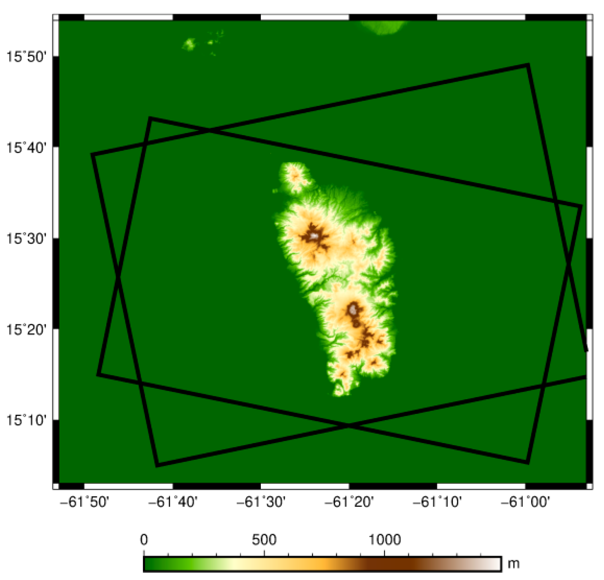
This study used seventy-seven ascending and descending single-look complex (SLC), wide multi-look fine, RADARSAT-2 (RS2) SAR datasets spanning April 2014 to June 2018. Their details are summarized in Table 1. A 10 m resolution DEM was used via [42]. The spatial coverage of the SAR and DEM datasets is shown in Figure 3. Data processing was performed using the DInSAR approach through GAMMA software [44]. The post processing was performed with the program provided by [45]. The application of both the SBAS technique, based on the work presented in [46,47], and the MSBAS process from [48], was used.
The data were preprocessed using MacDonald, Dettwiler and Associates’ Enhanced Definitive Orbit Tool (EDOT) to update the orbit vectors. EDOT uses raw Global Positioning System (GPS) data and provides an overall accuracy less than 1 m [49]. After the orbit vectors are updated, the perpendicular baselines between all non-redundant pairs of SLCs are calculated. A master image from each dataset is selected, 4 × 4 multi-looked, and geocoded to the DEM. The corresponding stacks of SLCs are then co-registered to their masters using look-up-table (LUT) refinement. A DEM in range Doppler coordinates (RDC) was also produced from each dataset.
Phase difference images, known as complex interferograms, were generated (from each dataset) using all non-redundant pairs of co-registered SLCs. The magnitude of the interferograms is a measure of coherence and represents the accuracy of the phase, while the interferometric phase represents a summation of the curved Earth, topography, deformation, atmospheric, and other phase noise components, as represented in Equation (1).
Δφ = φcurved Earth + φtopography + φdeformation +φatmospheric noise + others
The components of phase related to the Earth’s curvature (φcurved Earth) and topography (φ topography) are simulated and removed using the DEM (in RDC) and baselines. The results are differential interferograms (DIs). DIs contain inherent noise due to the geometry of the baseline, changes in temporal backscattering (i.e., changes in vegetation or land cover between acquisitions), thermal noise, and scene rotation [50]. Common-band filtering (including for both the range and azimuth spectra) was applied to improve correlation, while the adaptive filter purposed by [51] was applied to smooth out the interferometric fringes. For the adaptive filter, a correlation estimation window size of 5 pixels was used, along with a non-linear filter exponent of 0.2 (the lower end of the nominal range), and a Fast Fourier Transform filtering size of 16 (to take into account the rugged terrain). These values were selected based on the recommendations within the GAMMA software for Dominica’s terrain morphology.
The interferometric phase is cyclic in nature (it repeats every 2π), i.e., it is wrapped. To recover the absolute phase, phase unwrapping was applied. This is the method of adding or subtracting an integer value (n) of 2π to the phase of each neighbouring pixel [52]. As there is no unique solution (without added information), unwrapping is a mathematically ill-posed problem [53]. Accurate phase unwrapping is therefore crucial in InSAR processing. In this study, phase unwrapping was performed using an unwrapping mask (using a coherence threshold of 0.35) with minimum cost flow and Delaunay triangulation analysis. This phase unwrapping methodology has been shown to be suitable for the level of coherence obtained over Dominica [54].
From the unwrapped DI and DEM in RDC, the initial baseline estimate was refined based on the relationship between phase and topography, as represented in Equation (2) [55], where ϕtopo, Bn, λ, R, θ, and z represent the unwrapped phase, perpendicular baseline, radar wavelength, distance between the sensor and the target, look angle, and elevation, respectively. By taking a set of points on a grid, polynomial coefficients of the baseline may be determined through minimum least-squares estimation. Once the baselines are refined, the process of generating DIs is repeated. Based on the level of coherence, the DIs that contained consistently coherent pixels were selected for further processing.
The unwrapped DIs represent line-of-sight (LOS) deformation that has occurred between the two SAR acquisitions, as well as atmospheric and other noise components. They also include residual topography as a result of inaccuracies in the DEM used in the topographic phase removal [47]. The objective therefore becomes to minimize or remove these noise components to gain a more accurate deformation measurement. This was performed using the SBAS technique, which utilizes multi-master DI combinations with small temporal and perpendicular baselines [33]. As discussed in [47], the atmospheric phase component is assumed to contain all other random noise. The atmospheric (and other noise) components are estimated and removed through calibration. Equation (3) from [47] is then used to simultaneously solve for both the deformation rates between acquisitions, and the residual topography.
In Equation (3), A is a matrix that represents the associated time intervals (consecutive) between the DIs, V is the unknown velocity vector corresponding to the deformation rates, and ϕ is the observed DI phase vector. The unknown residual topography term is added to the velocity vector V. Linear least-squares inversion via singular value decomposition is then applied to solve for V. Knowing the deformation rates between acquisitions, the LOS cumulative displacement may be reconstructed through integration (as discussed next and shown in Equation (5)). This provides nonlinear LOS deformation time-series (for more detailed discussion, see [47]). The results were re-projected and converted to lat/long LOS deformation in metres with 10 m spatial sampling.
An extension of SBAS is the MSBAS process. MSBAS uses data from ascending and descending orbits to obtain time-series deformation in both the vertical and east-west directions [48], as calculated with Equation (4) from [48].
The matrix  = {sEA,sUA}, where A is the associated time intervals as described in Equation (3), and sE and sU are the corresponding LOS vector components in the east (E) and up (U) directions. The velocity vector V contains the unknown E and U velocities, while is the observed DI phase. The regularization parameter λ is used to smooth out the results, while L is a difference operator that controls the regularization order. Singular value decomposition is then applied to solve for the velocity vector at each pixel that remains coherent throughout the stack of interferograms. Once the E and U velocities are determined, the cumulative time-series deformation maps in the east-west and up-down directions are computed from Equation (5) from [48]. Here, d represents the deformation, N represents the total number of time intervals, and Δt is the time difference between corresponding acquisition pairs. For a more detailed explanation and thorough illustration of this process, see [48].
4. Results and Discussion
Dominica is a densely forested tropical island. Its steep rugged terrain and thick vegetation impact satellite spatial coverage and image-to-image coherence, respectively. Due to the satellite viewing geometry, the steep terrain introduces artifacts into the SAR data (foreshortening and layover). Slope faces that are visible from the ascending pass may not be visible from the descending pass, and vice-versa. This limits the spatial coverage when using the MSBAS technique (as it is dependent on there being coherence within both the ascending and descending datasets), and it restricts the use of ascending or descending passes to the slope orientation.
InSAR-SBAS processing is also dependent on coherence. Within the 2014 to 2018 range of SAR acquisitions used in this study, two major storm events occurred that dramatically altered the landscape due to extensive landslides and flooding. This led to a dramatic reduction in coherence. To mitigate these difficulties, the selection of orbit pass and DIs for each application studied was performed based on the slope and aspect of the terrain, and the dates of the Tropical Storm Erika and Hurricane Maria events. In addition, the selection of DIs was restricted to consecutive acquisition dates to ensure maximum coherence/spatial coverage. Dominica’s dense vegetation also limits coherence. Therefore, the InSAR results of this study reflect the coherent parts within the landslide (or slope), and not the entire landslide area. To note, the location of the reference point for each InSAR dataset was calculated automatically using a Z-Score approach. Additionally, the SBAS and MSBAS results represent relative deformation. For more accurate results, a known stable reference point would be required.
4.1. Identifying and Monitoring Landslide Activity
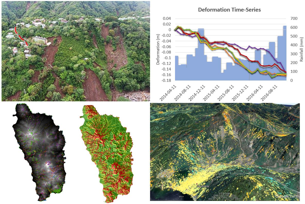
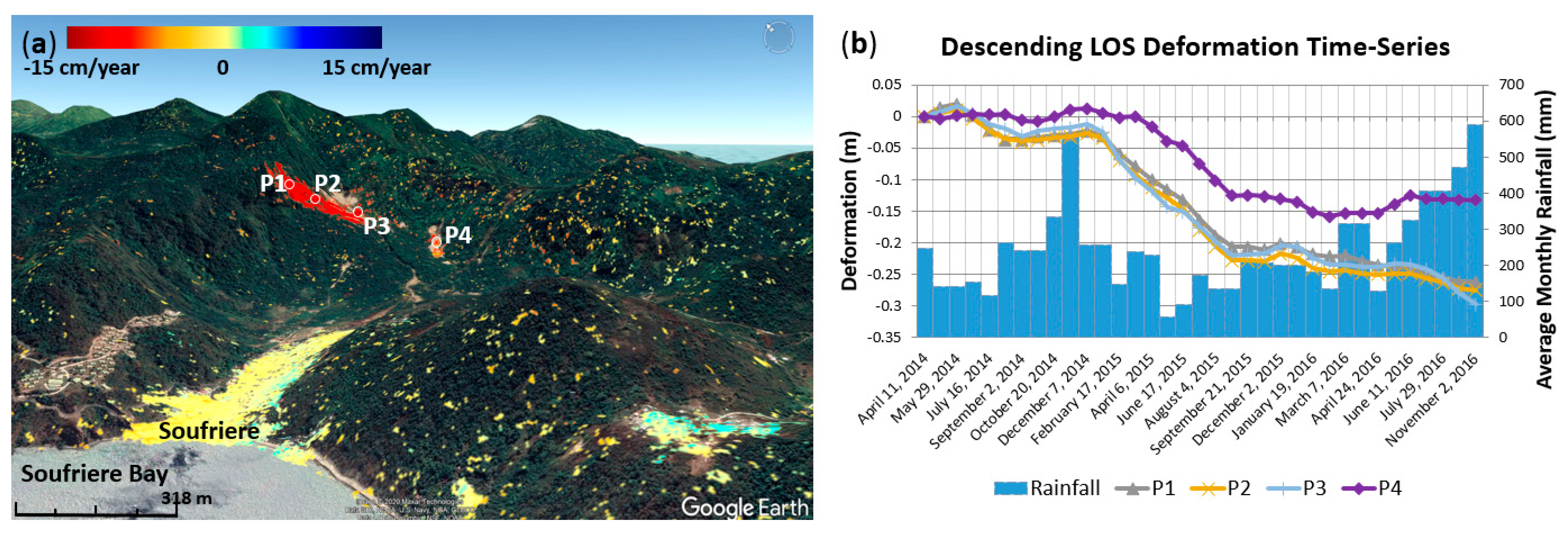
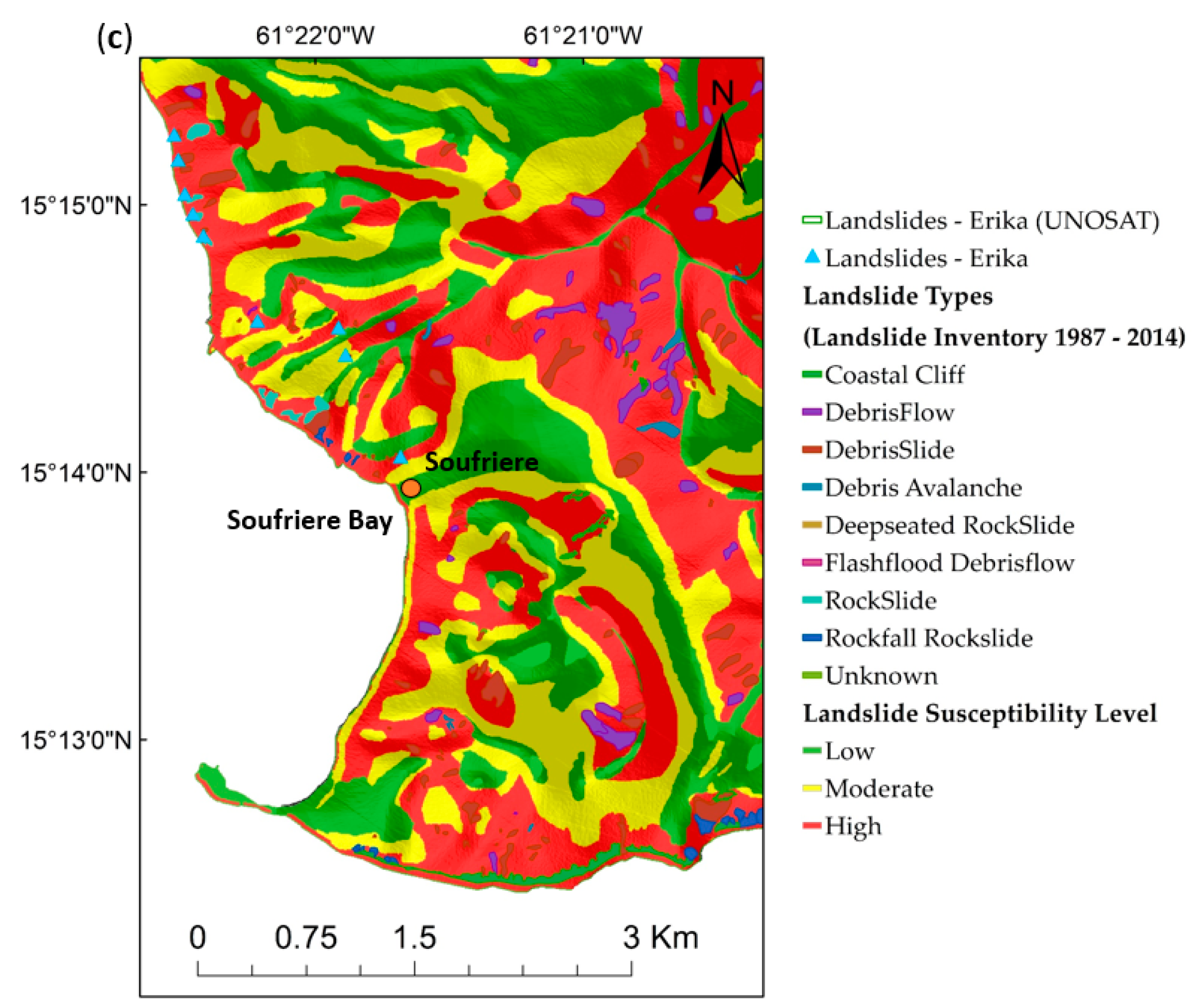
Figure 4 shows the April 2014 to November 2016 descending LOS deformation-rate map (or motion map) obtained from SBAS processing over the upper slopes surrounding the village of Soufriere. The results are overlain on Google Earth and include time-series analysis integrated with average monthly rainfall data. In the figure, there is also a segment of the 2016 landslide susceptibility map (produced after Tropical Storm Erika and before Hurricane Maria) over the same area illustrating the estimated risk of slope failure. The red colours in the deformation-rate map illustrate subsidence, while the blue colours represent uplift. The green areas in the susceptibility map show low risk zones where landslides are unlikely to take place, but may occasionally occur. The yellow areas represent moderate risk zones where landslides may occur, and the red areas represent zones where landslides are most likely to occur.
From satellite SAR data, InSAR motion maps can be used to identify areas at high risk by distinguishing between sites that are stable from those that are undergoing current slope instability. From the InSAR motion map in Figure 4a, for example, the yellow areas within the slopes are demonstrating stability, while the red areas are showing gradual motion of the parts of the slopes where potential landslides can occur when triggered by high rainfall. This map therefore highlights the areas within the slopes that are most at risk. These red and yellow areas correlate well with the corresponding susceptibility map in Figure 4c. Areas indicating notable subsidence or relative stability align with the red and green zones, respectively. In addition, our InSAR motion map, which focusses on the active slopes within the high landslide density areas, shows an active landslide recognized by InSAR (P1, P2, and P3, for example). Identifying active landslides, and highlighting areas most at risk from the InSAR motion map, allows it to be used to validate and update (if needed) the susceptibility map. The correlations between these two maps further confirm which areas are at greatest risk of landslide.
When creating a landslide inventory map, it is important to know when the landslides occurred. This is carried out to properly link the landslides with their triggering event in order to better predict future landslide risk from similar events. For slow-moving landslides, InSAR time-series analysis can be used to narrow down the time-period of when the slope initially begins to fail. When integrated with rainfall data (or landslide triggering events), the connection between the initiation of deformation and rainfall (or triggering event) may be analyzed. From the time-series analysis and rainfall data illustrated in Figure 4b, for example, the time-period for when the deformation was initiated for all points was observed to be between the December 2014 and January 2015 acquisitions. This deformation was shown to be initiated shortly after a significantly rainy month (November) in 2014. From this data, it is therefore suggested that the landslide observed at points P1–P3 was initiated between the end of 2014 and the start of 2015, and that heavy rainfall from the month of November 2014 may be the triggering event. Additional information regarding the variability in deformation behavior between the four points is also illustrated in Figure 4b. All points, for example, are shown to be relatively stable throughout the 2014 acquisitions. After the possible triggering event, each point shows subsidence, with P1–P3 subsiding at a faster rate than P4. P4 is then shown to be relatively stable throughout 2016, while P1–P3 continuously subside at different rates. This type of information provides a better understanding of the slope behaviour before and after the initiation of subsidence. Ref. [57] have shown similar motion on different parts of the island.
The back-monitoring capability from InSAR, when integrated with rainfall data (or data corresponding to known landslide triggering events), provides key information regarding the timespan of when the slope initially begins to fail, while also assisting with the identification of the potential landslide trigger—both of which are highly useful when producing inventory and susceptibility maps. It is worth noting that periodically applying InSAR on a regional scale for landslide monitoring, and then manually analyzing the time-series analysis for each point, may be difficult due to the large volume of data. Semi-automated approaches have been successfully implemented to address this challenge in relation to using DInSAR for geohazard activity assessment [58].
4.2. Slope Conditions Prior to Failure
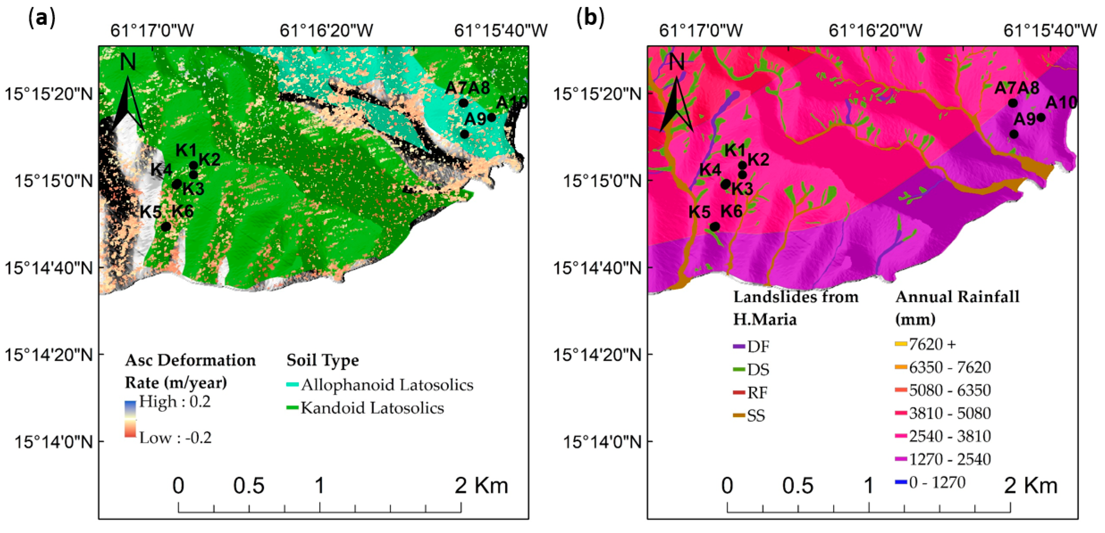
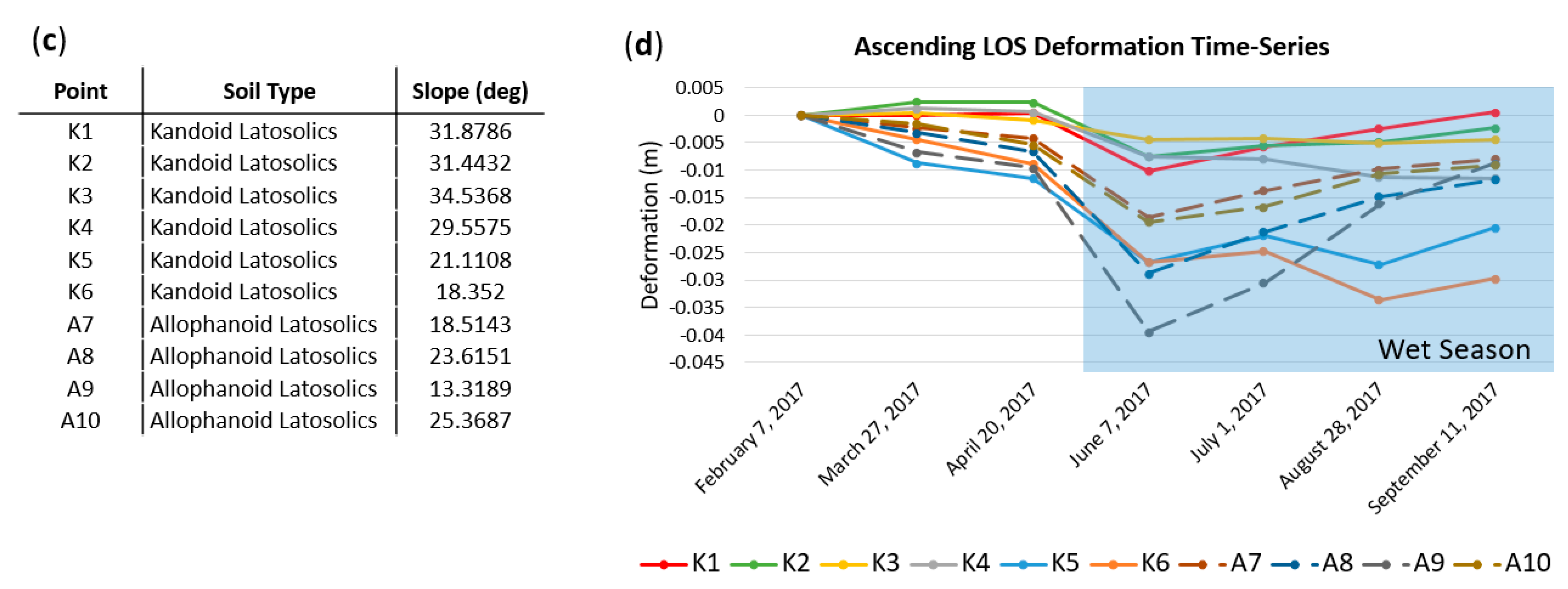
InSAR motion maps with time-series analysis can be used to facilitate a deeper understanding of the state of the slope prior to failure. Understanding pre-landslide conditions is essential as they are used to establish indicators for future risk when producing landslide susceptibility maps. Typical indicators that are used include slope, soil type and thickness, elevation, and annual rainfall amount. With InSAR, an additional indicator, such as slope motion behaviour observed prior to the initiation of slope failure, could be used. These behaviours may include whether or not the slope was stable, subsiding, or demonstrating uplift, and at what rates and time of year there was motion. This information can then be integrated with other parameters for a more robust understanding of pre-landslide conditions. An example of this is illustrated through Figure 5, which shows the results of applying the SBAS technique to ascending DIs from February to September 2017 over the southeastern area of the island. This dataset comprises the six months of acquisitions prior to Hurricane Maria. Figure 5a is a subset of the ascending LOS annual deformation-rate map overlaying the main soil types. Figure 5b is the mapped landslides triggered by Hurricane Maria overlaying the annual rainfall within the same area. Both images are overlaying a shaded relief. Within both images are ten points selected for time-series analysis. Points K1 to K6 are within the kandoid latosolic clays, and points A7 to A10 are in the allophanoid latosolics. All points are from areas that experienced debris slides (DS) from Hurricane Maria.
From the time-series in Figure 5d, the different deformation behaviour of each point prior to failure is observed. Points K1–K4 are shown to be stable until the start of the wet season. The other points show a slow rate of subsidence prior to the wet season, after which their rates of subsidence accelerate. All the points either remain stable after the June acquisition, or begin to demonstrate uplift. Through linking these site-specific patterns to other indicators used in future landslide risk assessment, such as slope and soil type, a more detailed analysis of the pre-landslide state may be established. For example, based on soil type, the kandoid clays and allophane latosolics are shown to be displaying similar trends, with the allophane latosolics showing an overall greater magnitude of deformation. With the addition of the slope information, it appears that the clay soils showing the greatest deformation are also the areas with the shallower slopes. This is observed within both the allophane latosolics and kandoid clay soils. For the allophane latosolics, point A9 has the shallowest slope (~13 degrees) and the greatest deformation (up to 4 cm in subsidence before showing uplift). Within the kandoid clays, points K5 and K6 have the shallowest slopes (18 to 21 degrees) while also demonstrating the greatest deformation (subsidence over 2.5 cm).
As discussed by [8], the allophane latosolics and kandoid clays have similar properties, but differ within the saturation conditions at the soil/rock interface (kandoid clays were at or near saturation in this zone during the wet season, whereas allophane clays were perennially saturated). Significant rainfall was determined to be required to overcome the increasingly impermeable subsoil layers, and lateral throughflow, to induce slope failure at the soil/rock interface [8]. From the results in Figure 5, the points with the shallower slopes display the most subsidence prior to failure. This may suggest that the higher slopes help in the lateral throughflow, thereby requiring higher amounts of rainfall to induce instability within these areas (more work is needed to better understand this observation). The difference in saturation conditions at the soil/rock interface between the two soil types may also help explain why the allophane areas showed a greater magnitude of deformation over the kandoid clays. Despite these differences, each site failed due to the effects of Hurricane Maria. Understanding their differences could assist in better understanding pre-landslide conditions. Pre-landslide slope movement or behaviour patterns from InSAR, integrated with soil type and slope, could be included in the list of indicators used in the prediction of future landslide risk.
4.3. Slope Conditions Post Failure
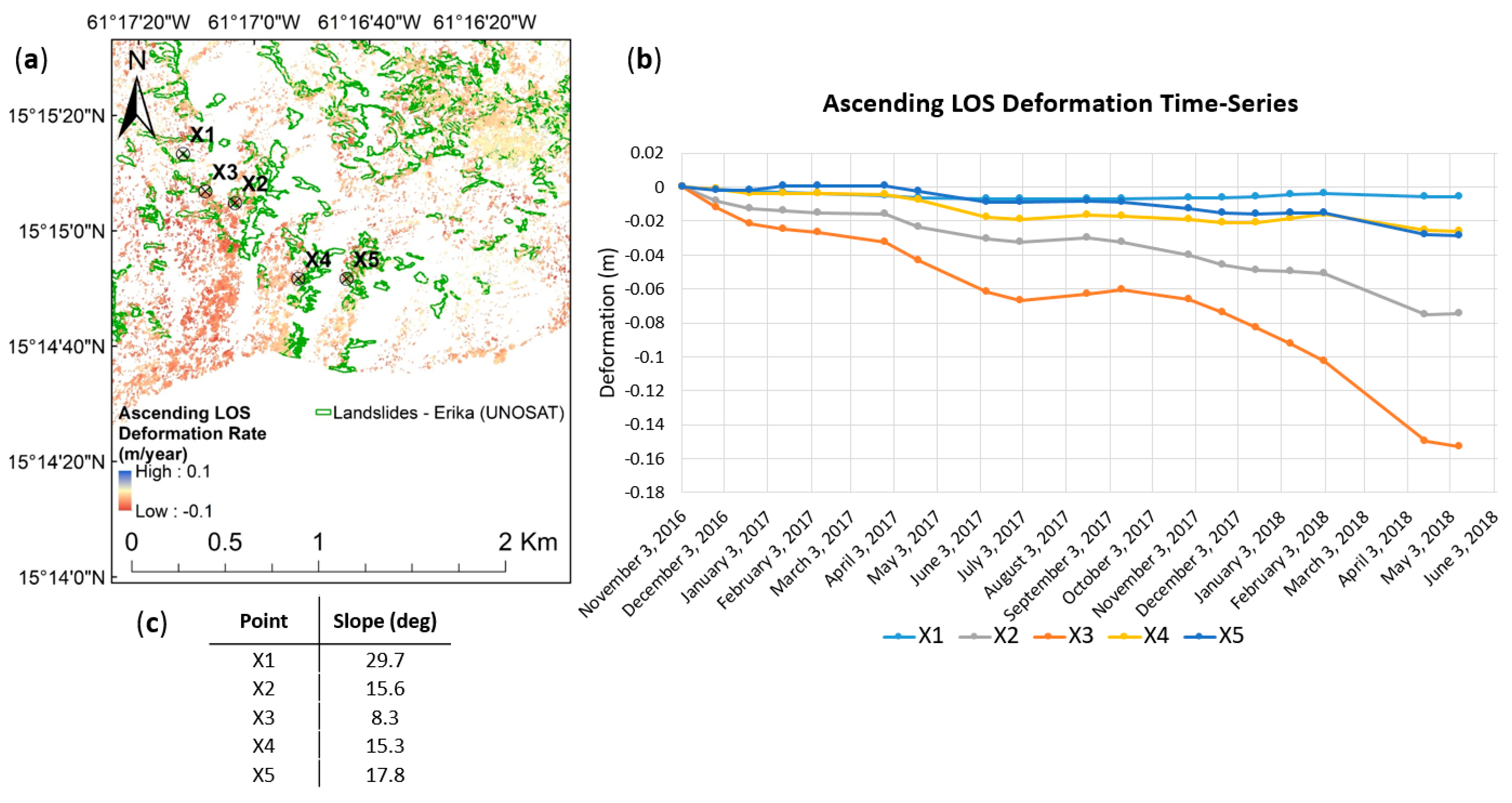
When making the inventory map, the landslides recorded from each mapping session are added together and used in part to create the susceptibility map. The inventory map overlaying the susceptibility map in Figure 4c, for example, is generated based on the landslides recorded from inventories conducted in 1987, 1990, 2007, 2014, and 2015. Using InSAR, the activity levels of these landslides may be monitored. This information can assist in the classification of these landslides as being either active or dormant. Knowing which areas are active can facilitate a more targeted approach for the implementation of landslide mitigation strategies, as well as be used as additional indicators in the production of the susceptibility map. Figure 6 is shown as an example of using InSAR for post-landslide monitoring. Illustrated in the figure are the results of applying the SBAS technique to the ascending DIs ranging from November 2016 to May 2018. This set of data represents roughly a year and a half post-Tropical Storm Erika (and pre-Hurricane Maria). The InSAR results are integrated with the recorded Tropical Storm Erika-induced landslides. The five points selected within these landslides (points X1–X5) are highlighted in the figure. Figure 6b,c shows the slope values and time-series analysis of each point.
From the graph in Figure 6b, points X1, X4, and X5 demonstrate stability from the end of 2016 to at least mid-2018, suggesting those landslides are more dormant than active. The landslides associated with X2 and X3, however, are shown to be relatively active. Similar to the findings from Figure 5, from the two active landslides, the one with the shallower slope (X3 at 8.3 degrees) is shown to be deforming at a faster rate than the one with a steeper slope (X2 at 15.6 degrees). Identifying active sites allows for targeted fieldwork, landslide mitigation strategies, and intense monitoring programs to be initiated to reduce the landslide risk. We recommend that InSAR motion indicators should be an additional layer on future landslide susceptibility maps to improve visualization and interpretation in the determination of potential landslide risk.
4.4. Kinematic Behaviour
In addition to supporting inventory and susceptibility mapping, InSAR data, when generated through the MSBAS approach, can provide further details of land deformation, such as terrain kinematics. While the SBAS approach provides deformation in the LOS, up/down (U/D) direction, the MSBAS approach, which utilizes the ascending and descending data together, can provide an additional dimension of motion in the east/west (E/W) direction. This allows MSBAS data to be used to assist in determining whether the land is predominantly moving in the vertical U/D direction, E/W direction, or, to what extent, a mixture of both. To note, the traditional MSBAS approach cannot measure motion in the North/South direction. This limitation is discussed in Section 4.6.
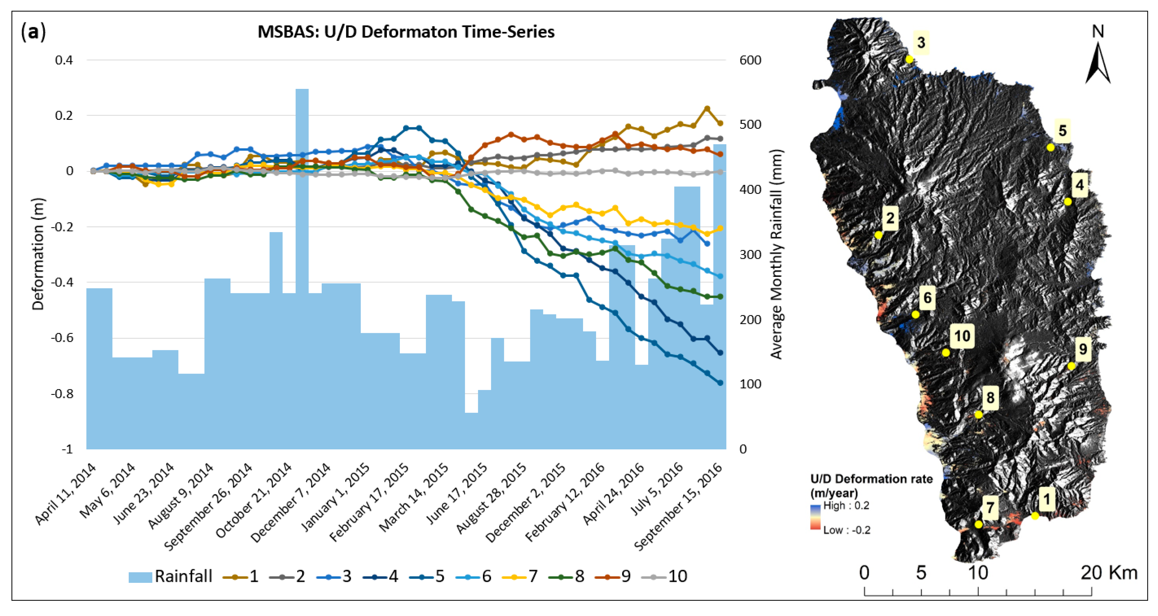
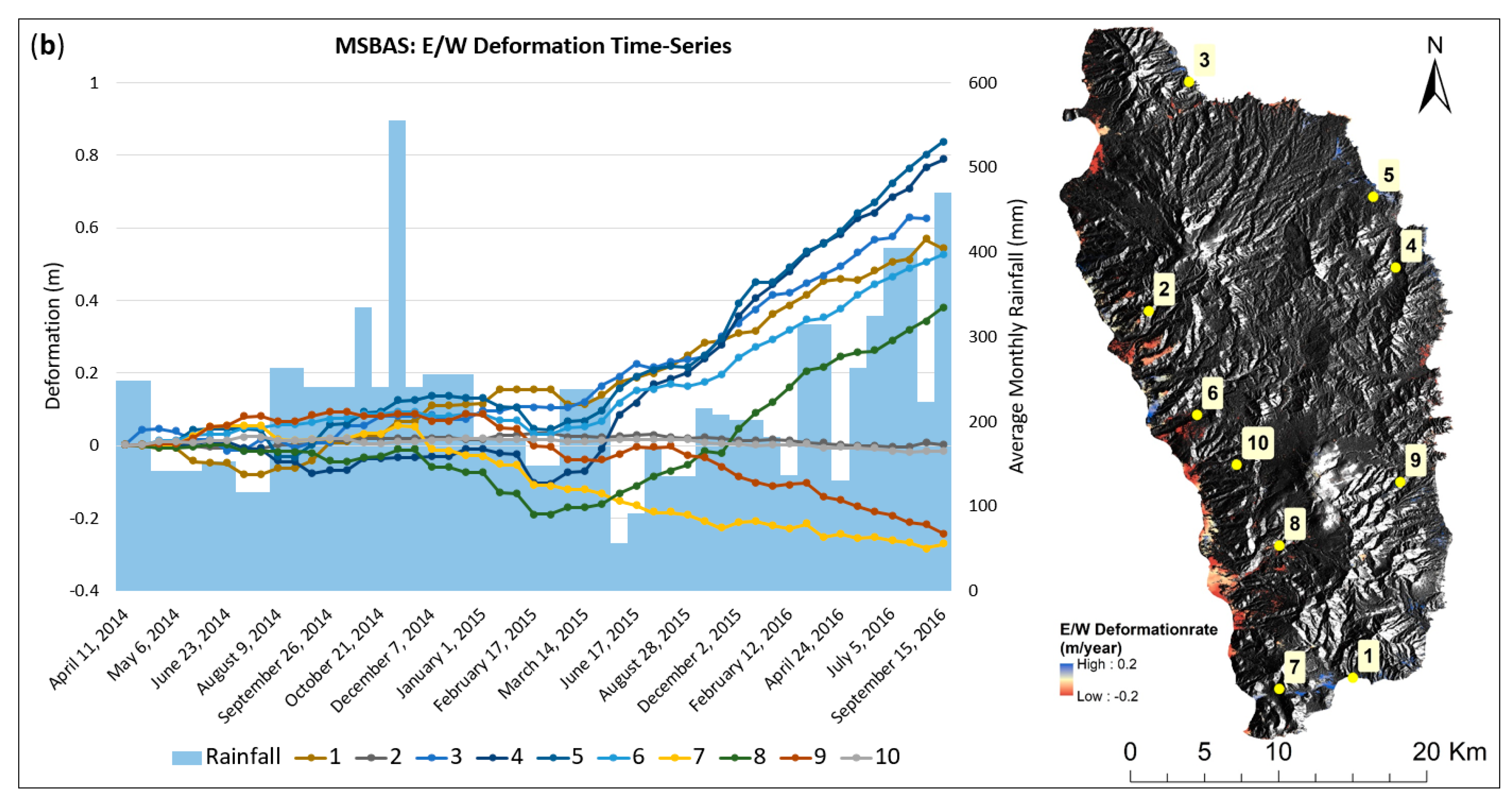
Figure 7 shows the MSBAS results over the island using ascending and descending data acquired between April 2014 and September 2016. Figure 7a is the deformation-rate map of the component of motion in the U/D direction, alongside the corresponding time-series of the ten points highlighted. Figure 7b is the corresponding data for the component of motion in the E/W direction. The blue colours represent up and east, while the red colours represent down and west. Illustrated in the time-series of the figure are the differential deformation rates and two-dimensional direction of motion of the ten points highlighted. From this data, it can be shown that point 1 is mostly moving east at a relatively slow rate, while point 9 is mainly moving west at a faster rate. Some locations are showing a relatively even mixture of moving down as well as east (points 4 and 5, for example), at relatively fast rates in both directions. Points 2 and 10 are shown to be relatively stable in both directions. These types of details can be utilized for a better understanding of the kinematic behaviour of the terrain, which would facilitate a more effective implementation of targeted landslide mitigation strategies. Due to the ruggedness of the island, however, the spatial extent of the MSBAS data is limited in comparison to the SBAS results (as discussed at the beginning of Section 4). As the MSBAS data provides highly beneficial information, using different viewing geometries may improve their use for high relief terrain, as occurs at Dominica.
4.5. Landslide Rainfall Threshold
In addition to better understanding the pre-landslide conditions for use in the prediction of future landslide risk, landslide-inducing rainfall thresholds are also used [59,60,61,62]. For Dominica, a rainfall threshold was calculated by linking daily rainfall measurements (between 1977 and 2013) recorded from two rain gauges (one on the east side of the island, and one on the west side) with the days in which landslides were documented [6]. Within the resulting dataset, there were a high number of rainfall events with no associated landslides, representing false alarms. Ref. [6] speculated that this was due to both the underreporting of landslide occurrences (lack of historical landslide data) and the lack of rain gauges. As discussed in Section 2, the amount of rainfall varies greatly with respect to elevation (Figure 2d), and it is therefore likely that the location of the two rainfall gauges used did not adequately reflect the amount of rainfall that occurred in the areas with recorded landslides.
In addition to the lack of historical landslide data, calculating a rainfall threshold is considerably difficult due to the variability in the selection of the number of antecedent rainfall days to use [63]. Ranges from 1 to 15 days [64,65] to an accumulation of 180 days [66,67] have been recommended. Ref. [6] used 5 days for the threshold in Dominica. Narrowing down upper and lower limits of the number of antecedent days to use may improve the rainfall threshold estimate. Using InSAR back-monitoring, the time-period when the initial land subsidence occurred may be narrowed down. This information can then be linked to the date of the rainfall event and then used to constrain the selection of the number of antecedent days to use. Figure 4b, for example, illustrates that after the heavy rainfall month recorded in November 2014, the initiation of subsidence was observed at the 31 December 2014 acquisition. This may suggest that slow-moving landslides, with these particular terrain characteristics (i.e., slope geometry, soil type, annual rainfall, etc.), may be initiated up to a month after heavy rainfall. Compiling an historical database of these types of measurements under different environmental conditions would assist in the refinement of the number of antecedent rainfall days to use over the various terrains, and provide statistical reliability of the analysis. With the recent launch of Canada’s RADARSAT Constellation Mission (RCM), revisit times of up to 4 days may be achieved. This is a notable increase over RS2′s 24 day revisit period. Using RCM data, the upper and lower limits of the number of antecedent days to use could be substantially constrained.
4.6. InSAR Limitations
There are many benefits to the use of SAR data for landslide risk assessment. However, there are some limitations. The observable rate of deformation is restricted by the wavelength of the SAR sensor used. Rapidly moving catastrophic landslides (as shown in Figure 1) may have deformation rates well in excess of metres per minute. This extreme rate of motion cannot be directly observed from today’s SAR satellites. As calculated from [34], the maximum observable rate of deformation for RS2′s 5.5 cm C-band is 2.3 mm/day. Increasing the wavelength or decreasing the revisit cycle would increase this rate. RCM, for example, with its rapid revisit, would allow for the monitoring of faster moving landslides, with deformation rates of up to 13.75 mm/day being possible. As satellite revisit times continue to decrease, this deformation rate limitation further highlights the necessity for better understanding and monitoring pre-failure conditions.
Another limitation is dense vegetation. Areas with higher densities of vegetation lead to an increase in volumetric decorrelation, which limits coherence [68]. Installing corner reflectors on the most serious or worrisome vegetated slopes, using longer wavelengths such as L-band that can penetrate vegetation, and/or increasing the temporal resolution would increase coherence. However, longer wavelengths (such as L-band) can introduce significant atmospheric delay. Without the use of complex atmospheric mitigation algorithms, this may lead to erroneous deformation measurements.
In addition, deformation in the north/south direction cannot be measured using the traditional MSBAS approach [48]. As surface motion occurs in three dimensional space (up/down, east/west, and north/south), the true direction and magnitude of movement are therefore not measured. This is a result of the lack of variability in the ascending and descending North-South orbital plane [69]. This may be overcome by using satellite SAR data acquired from three different viewing (orbital) geometries, or through the integration of satellite SAR data with airborne SAR (as its azimuth direction is easily controllable) [48].
5. Conclusions
There is an increasing need for landslide disaster risk mitigation efforts within Dominica due to the growing impacts from tropical storms and hurricane events. Landslide inventory and susceptibility maps are considered critical to landslide risk assessment. In Dominica, these maps are currently generated from optical imagery, digital elevation models, and historical landslide data. In this study, we show how InSAR deformation-rate maps and time-series analysis may be used to update inventory maps and improve susceptibility maps in a highly rugged, tropical environment. The results of this study show differential rates of landslide motion before and after major storm events. We show active and stable areas identified using InSAR motion maps, as well as identify relatively continuously active and inactive landslides after a major storm event. We observe more land motion prior to failure on clay soils with gentler slopes than on those with steeper slopes (the reason for this needs to be investigated further), and we show a delay in land subsidence (over numerous sites) after a significantly rainy period from our time-series analysis. These results will improve inventory and susceptibility mapping to better highlight areas at risk, contribute to the understanding of pre-slope failure characteristics, support the development of rainfall thresholds for different terrains, and further the monitoring of kinematic behaviour. More efficient infrastructure planning and development programs may then be implemented to reduce the impact of future major storm and heavy rainfall events.
Author Contributions
Conceptualization, V.S.; methodology, M.-A.F.; software, M.-A.F.; validation, V.S.; formal analysis, V.S.; investigation, M.-A.F.; resources, V.S.; data curation, M.-A.F.; Writing—Original draft preparation, M.-A.F.; Writing—Review and editing, M.-A.F., J.G.S. and V.S.; supervision, V.S. and J.G.S.; project administration, J.G.S.; funding acquisition, V.S. All authors have read and agreed to the published version of the manuscript.
Funding
This work has been supported by a Natural Sciences and Engineering Research Council of Canada Discovery grant awarded to J.S.
Acknowledgments
Ancillary data were obtained from CHARIM (http://charim-geonode.net accessed on 6 January 2021). RADARSAT-2 data were accessed through the Canada Centre for Remote Sensing (CCRS). The authors would like to thank CCRS for their support, and for the constructive evaluation from all the anonymous reviewers.
Conflicts of Interest
The authors declare no conflict of interest.
References
- Howe, T.M.; Lindsay, J.M.; Shane, P. Evolution of young andesitic-dacitic magmatic systems beneath Dominica, Lesser Antilles. J. Volcanol. Geotherm. Res. 2015, 297, 69–88. [Google Scholar] [CrossRef]
- Government of the Commonwealth of Dominica. Post Disaster Needs Assessment Hurricane Maria September 18, 2017. Government of the Commonwealth of Dominica: Roseau, Dominica, 2017; pp. 1–17. [Google Scholar]
- Barclay, J.; Wilkinson, E.; White, C.S.; Shelton, C.; Forster, J.; Few, R.; Lorenzoni, I.; Woolhouse, G.; Jowitt, C.; Stone, H.; et al. Historical trajectories of disaster risk in Dominica. Int. J. Disaster Risk Sci. 2019, 10, 149–165. [Google Scholar] [CrossRef] [Green Version]
- Fontaine, G. Multi-Hazard Early Warning Systems Gaps Assessment Report for the Commonwealth of Dominica; Dominica Emergency Management Organization: Roseau, Dominica, 2018. [Google Scholar]
- Climate Watch. 2020. Available online: https://www.climatewatchdata.org (accessed on 7 July 2020).
- Van Westen, C.J. National Scale Landslide Susceptibility Assessment for Dominica. World Bank Caribb. Handb. Risk Inf. Manag. Tech. Rep. 2016. [Google Scholar] [CrossRef]
- Lugo, A.E.; Applefield, M.; Pool, D.J.; McDonald, R.B. The impact of Hurricane David on the forests of Dominica. Can. J. For. Res. 1983, 13, 201–211. [Google Scholar] [CrossRef]
- Rouse, W.C.; Reading, A.J.; Walsh, R.P.D. Volcanic soil properties in Dominica, West Indies. Eng. Geol. 1986, 23, 1–28. [Google Scholar] [CrossRef]
- Nugent, A.D.; Rios-Berrios, R. Factors leading to extreme precipitation on Dominica from Tropical Storm Erika (2015). Mon. Weather. Rev. 2018, 146, 525–541. [Google Scholar] [CrossRef]
- Ogden, F.L. Evidence of equilibrium peak runoff rates in steep tropical terrain on the island of Dominica during Tropical Storm Erika, August 27, 2015. J. Hydrol. 2016, 542, 35–46. [Google Scholar] [CrossRef] [Green Version]
- Rapid Damage and Impact Assessment Tropical Storm Erika—August 27, 2015; Government of the Commonwealth of Dominica: Roseau, Dominica, 2015.
- BBC News in pictures: Dominica Rebuilds after Storm Erika. Available online: https://www.bbc.com/news/world-latin-america-34244043 (accessed on 7 July 2020).
- The Sun Pettie Savanne—Anatomy of the Disaster. Available online: http://sundominica.com/galleries/petite-savanne-anatomy-of-the-disaster-70/#/0 (accessed on 7 July 2020).
- United Nations Institute for Training and Research Tropical Cyclone Maria Inventory of Landslides and Flooded Areas. Available online: http://www.unitar.org/unosat/node/44/2762 (accessed on 15 March 2020).
- Feringa, W.; Thomas, P. Caribbean Handbook on Risk Information Management (CHARIM). Available online: http://www.charim.net/ (accessed on 7 July 2020).
- Dai, F.C.; Lee, C.F.; Ngai, Y.Y. Landslide risk assessment and management: An overview. Eng. Geol. 2002, 64, 65–87. [Google Scholar] [CrossRef]
- Van Westen, C.J.; Castellanos, E.; Kuriakose, S.L. Spatial data for landslide susceptibility, hazard, and vulnerability assessment: An overview. Eng. Geol. 2008, 102, 112–131. [Google Scholar] [CrossRef]
- Aleotti, P.; Chowdhury, R. Landslide hazard assessment: Summary review and new perspectives. Bull. Eng. Geol. Environ. 1999, 58, 21–44. [Google Scholar] [CrossRef]
- Hu, T.; Smith, R.B. The impact of Hurricane Maria on the vegetation of Dominica and Puerto Rico using Multispectral Remote Sensing. Remote Sens. 2018, 10, 827. [Google Scholar] [CrossRef] [Green Version]
- Tomás, R.; Li, Z.; Liu, P.; Singleton, A.; Hoey, T.; Cheng, X. Spatiotemporal characteristics of the Huangtupo landslide in the Three Gorges region (China) constrained by radar interferometry. Geophys. J. Int. 2014, 197, 213–232. [Google Scholar] [CrossRef] [Green Version]
- Schlögel, R.; Doubre, C.; Malet, J.P.; Masson, F. Landslide deformation monitoring with ALOS/PALSAR imagery: A D-InSAR geomorphological interpretation method. Geomorphology 2015, 231, 314–330. [Google Scholar] [CrossRef]
- Nishiguchi, T.; Tsuchiya, S.; Imaizumi, F. Detection and accuracy of landslide movement by InSAR analysis using PALSAR-2 data. Landslides 2017, 14, 1483–1490. [Google Scholar] [CrossRef]
- Bouali, E.H.; Oommen, T.; Escobar-Wolf, R. Mapping of slow moving landslides on the Palos Verdes Peninsula using the California landslide inventory and persistent scatterer interferometry. Landslides 2018, 15, 439–452. [Google Scholar] [CrossRef]
- Rosi, A.; Tofani, V.; Tanteri, L.; Stefanelli, C.T.; Agostini, A.; Catani, F.; Casagli, N. The new landslide inventory of Tuscany (Italy) updated with PS-InSAR: Geomorphological features and landslide distribution. Landslides 2018, 15, 5–19. [Google Scholar] [CrossRef] [Green Version]
- Virk, A.S.; Singh, A.; Mittal, S.K. Advanced MT-InSAR monitoring: Methods and trends. J. Remote Sens. GIS. 2018, 7. [Google Scholar] [CrossRef]
- Zhao, C.; Kang, Y.; Zhang, Q.; Lu, Z.; Li, B. Landslide identification and monitoring along the Jinsha River Catchment (Wudongde Reservoir Area), China, using the InSAR method. Remote Sens. 2018, 10, 993. [Google Scholar] [CrossRef] [Green Version]
- Roberts, N.J.; Rabus, B.T.; Clague, J.J.; Hermanns, R.L.; Guzmán, M.A.; Minaya, E. Changes in ground deformation prior to and following a large urban landslide in La Paz, Bolivia, revealed by advanced InSAR. Nat. Hazards Earth Syst. Sci. 2019, 19, 679–696. [Google Scholar] [CrossRef] [Green Version]
- Jia, H.; Zhang, H.; Liu, L.; Liu, G. Landslide deformation monitoring by adaptive distributed scatterer interferometric synthetic aperture radar. Remote Sens. 2019, 11, 2273. [Google Scholar] [CrossRef] [Green Version]
- Liu, X.; Zhao, C.; Zhang, Q.; Yang, C.; Zhu, W. Heifangtai loess landslide type and failure mode analysis with ascending and descending Spot-mode TerraSAR-X datasets. Landslide 2020, 17, 205–215. [Google Scholar] [CrossRef] [Green Version]
- Alimuddin, I.; Bayuaji, L.; Maddi, H.C.; Sumantyo, J.T.S.; Kuze, H. Developing tropical landslide susceptibility map using DInSAR technique of JERS-1 SAR data. Int. J. Remote Sens. Earth Sci. 2011, 8, 32–40. [Google Scholar] [CrossRef]
- Putri, R.F.; Wibirama, S.; Alimuddin, I.; Kuze, H.; Sumantyo, J.T.S. Monitoring and analysis of landslide hazard using DInSAR technique applied to ALOS PALSAR imagery: A case study in Kayanhan catchment area, Yogyakarta, Indonesia. J. Urban Environ. Eng. 2013, 7, 308–322. [Google Scholar] [CrossRef] [Green Version]
- Jebur, M.N.; Pradhan, B.; Tehrany, M.S. Detection of vertical slope movement in highly vegetated tropical area of Gunung pass landslide, Malaysia, using L-band InSAR technique. Geosci. J. 2014, 18, 61–68. [Google Scholar] [CrossRef]
- Casagli, N.; Cigna, F.; Bianchini, S.; Hölbling, D.; Füreder, P.; Righini, G.; Del Conte, S.; Friedl, B.; Schneiderbauer, S.; Iasio, C.; et al. Landslide mapping and monitoring by using radar and optical remote sensing: Example from the EC-FP7 project SAFER. Remote Sens. Appl. Soc. Environ. 2016, 4, 92–180. [Google Scholar] [CrossRef] [Green Version]
- Zhou, X.; Chang, N.B.; Li, S. Applications of SAR interferometry in Earth and environmental science research. Sensors 2009, 9, 1876–1912. [Google Scholar] [CrossRef] [Green Version]
- De Graff, J.V.; Romesburg, H.C.; Ahmad, R.; McCalpin, J.P. Producing landslide-susceptibility maps for regional planning in data-scarce regions. Nat. Hazards 2012, 64, 729–749. [Google Scholar] [CrossRef]
- Maitland, B.M.; O’Malley, B.P.; Stewar, D.J. Subsurface water piping transports plankton and prevents meromixis in a deep volcanic crater lake (Dominica, West Indies). Hydobiologia 2019, 839, 119–130. [Google Scholar] [CrossRef]
- Joseph, E.P.; Frey, H.M.; Manon, M.R.; Onyeali, M.C.; DeFranco, K.; Metzger, T.; Aragosa, C. Update on the fluid geochemistry monitoring time series for geothermal systems in Dominica, Lesser Antilles island arc: 2009–2017. J. Volcanol. Geotherm. Res. 2019, 376, 86–103. [Google Scholar] [CrossRef]
- Mayer, K.; Scheu, B.; Yilmaz, T.I.; Montanaro, C.; Gilg, H.A.; Rott, S.; Joseph, E.P.; Dingwell, D.B. Phreatic activity and hydrothermal alteration of Desolation, Dominica, Lesser Antilles. Bull. Volcanol. 2017, 79, 82. [Google Scholar] [CrossRef]
- Rouse, C. The mechanics of small topical flowslides in Dominica, West Indies. Eng. Geol. 1990, 29, 227–239. [Google Scholar] [CrossRef]
- Reading, A.J. Stability of tropical residual soils from Dominica, West Indies. Eng. Geol. 1991, 31, 27–44. [Google Scholar] [CrossRef]
- Benson, C.; Clay, E.; Michael, F.V.; Robertson, A.W. Disaster Risk Management Working Paper Series No. 2 Dominica: Natural Disasters and Economic Development in a Small Island State; World Bank: Washington, DC, USA, 2001; pp. 1–3. [Google Scholar]
- Feringa, W.; Thomas, P. Caribbean Handbook on Risk Information Management (CHARIM) GeoNode. Available online: http://charim-geonode.net/ (accessed on 7 July 2020).
- Government of the Commonwealth of Dominica. Physical Planning Division. Available online: http://physicalplanning.gov.dm/land-use-and-development/maps (accessed on 6 August 2020).
- Wegmüller, U.; Werner, C. Gamma SAR processor and interferometry software. In Proceedings of the 3rd ERS Symposium, Florence, Italy, 18–21 March 1997; pp. 1686–1692. [Google Scholar]
- Samsonov, S.V. User Manual, Source Code, and Test Set for MSBASv3 (Multidimensional Small Baseline Subset Version 3) for One- and Two-Dimensional Deformation Analysis, Open File 45; Natural Resources Canada: Ottawa, ON, Canada, 2019; pp. 1–13. [Google Scholar] [CrossRef]
- Berardino, P.; Fornaro, G.; Lanari, R.; Sansosti, E. A new algorithm for surface deformation monitoring based on the small baseline differential SAR interferograms. IEEE Trans. Geosci. Remote Sens. 2002, 40, 2375–2383. [Google Scholar] [CrossRef] [Green Version]
- Samsonov, S.; van der Kooij, M.; Tiampo, K. A simultaneous inversion for deformation rates and topographic errors of DInSAR data utilizing linear least square inversion technique. Comput. Geosci. 2011, 37, 1083–1091. [Google Scholar] [CrossRef]
- Samsonov, S.V.; d’Oreye, N. Multidimensional small baseline subset (MSBAS) for two-dimensional deformation analysis: Case study Mexico City. Can. J. Remote Sens. 2017, 43, 318–329. [Google Scholar] [CrossRef]
- Lambert, C.; Williams, D.; Eppler, J. RADARSAT-2 Definitive Orbit Upgrade, Report No. RN-MK-53-8119; MDA: Richmond, BC, Canada, 2015; pp. 11–12. [Google Scholar]
- Zebker, H.A.; Villasenor, J. Decorrelation in interferometric radar echoes. IEEE Trans. Geosci. Remote Sens. 1992, 30, 950–959. [Google Scholar] [CrossRef] [Green Version]
- Goldstein, R.M.; Werner, C.L. Radar interferogram filtering for geophysical applications. Geophys. Res. Lett. 1998, 25, 4035–4038. [Google Scholar] [CrossRef] [Green Version]
- Rani, K.; Shankar, A.V. Review on phase unwrapping techniques in interferometry. Int. J. Adv. Res. Electron. Commun. Eng. 2017, 6, 798–802. [Google Scholar]
- Zhou, L.; Chai, D.; Xia, Y.; Ma, P.; Lin, H. Interferometric synthetic aperture radar phase unwrapping based on sparse Markov random fields by graph cuts. J. Appl. Remote Sens. 2018, 12. [Google Scholar] [CrossRef] [Green Version]
- Zhang, B.; Li, J.; Ren, H. Using phase unwrapping methods to apply D-InSAR in mining areas. Can. J. Remote Sens. 2019, 45, 225–233. [Google Scholar] [CrossRef]
- GAMMA Remote Sensing. Documentation Theory Interferometric SAR Processing, Version 1.0; GAMMA Remote Sensing: Gümligen, Switzerland, 2007; pp. 9–11. [Google Scholar]
- World Bank Group Climate Change Knowledge Portal for Development Practitioners and Policy Makers. Available online: https://climateknowledgeportal.worldbank.org/download-data (accessed on 15 March 2020).
- Singhroy, V.; Li, J.; Fobert, M.; Lee, C.F.; Das, M.K. Monitoring post landslide activity from RADARSAT Constellation Mission. In Proceedings of the IGARSS 2019 IEEE International Geoscience and Remote Sensing Symposium, Yokohama, Japan, 28 July –2 August 2019. [Google Scholar] [CrossRef]
- Barra, A.; Solari, L.; Béjar-Pizarro, M.; Monserrat, O.; Bianchini, S.; Herrera, G.; Crosetto, M.; Sarro, R.; González-Alonso, E.; Mateos, R.M.; et al. A methodology to detect and update active deformation areas based on Sentinel-1 SAR images. Remote Sens. 2017, 9, 1002. [Google Scholar] [CrossRef] [Green Version]
- Martelloni, G.; Segoni, S.; Fanti, R.; Catani, F. Rainfall thresholds for forecasting of landslide occurrence at regional scale. Landslides 2012, 9, 485–495. [Google Scholar] [CrossRef] [Green Version]
- Peruccacci, S.; Brunetti, M.T.; Gariano, S.L.; Melillo, M.; Rossi, M.; Guzzetti, F. Rainfall thresholds for possible landslide occurrence in Italy. Geomorphology 2017, 290, 39–57. [Google Scholar] [CrossRef]
- Vaz, T.; Zêzere, J.L.; Pereira, S.; Oliveira, S.C.; Garcia, R.A.C.; Quaresma, I. Regional rainfall thresholds for landslide occurrences using a centenary database. Nat. Hazards Earth Syst. Sci. 2018, 18, 1037–1054. [Google Scholar] [CrossRef] [Green Version]
- He, S.; Wang, J.; Liu, S. Rainfall event-duration thresholds for landslide occurrences in China. Water 2020, 12, 494. [Google Scholar] [CrossRef] [Green Version]
- Guzzetti, F.; Peruccacci, S.; Rossi, M.; Stark, C.P. Rainfall thresholds for the initiation of landslides in central and southern Europe. Meteorol. Atmos. Phys. 2007, 98, 239–267. [Google Scholar] [CrossRef]
- Glade, T.; Crozier, M.; Smith, P. Applying probability determination to refine landslide-triggering rainfall thresholds using an empirical “antecedent daily rainfall model”. Pure Appl. Geophys. 2000, 157, 1059–1079. [Google Scholar] [CrossRef]
- Aleotti, P. A warning system for rainfall-induced shallow failures. Eng. Geol. 2004, 73, 247–265. [Google Scholar] [CrossRef]
- Polemio, M.; Sdao, F. The role of rainfall in the landslide hazard: The case of the Avigliano urban area (Southern Apennines, Italy). Eng. Geol. 1999, 53, 297–309. [Google Scholar] [CrossRef]
- Zêzere, J.L.; Trigo, R.M.; Trigo, I.F. Shallow and deep landslides induced by rainfall in the Lisbon region (Portugal): Assessment of relationships with the North Atlantic Oscillation. Nat. Hazards Earth Syst. Sci. 2005, 5, 331–344. [Google Scholar] [CrossRef]
- Pepe, A.; Calò, F. A review of interferometric synthetic aperture radar (InSAR) multi-track approaches for the retrieval of Earth’s surface displacements. Appl. Sci. 2017, 7, 1264. [Google Scholar] [CrossRef] [Green Version]
- Furhmann, T.; Garthwaite, M.C. Resolving three-dimensional surface motion with InSAR: Constraints from multi-geometry data fusion. Remote Sens. 2015, 11, 241. [Google Scholar] [CrossRef] [Green Version]
Figure 1.
Landslides triggered from Tropical Storm Erika in the village of Petite Savanne. (a) is from [12], while (b–d) are from [13]. The roads have been highlighted with red-dashed lines to illustrate the impact on the transportation infrastructure.

Figure 2.
(a) Geological age, (b) deposits, (c) elevation, and (d) annual rainfall amounts of Dominica overlaying a Digital Elevation Model (DEM) derived shaded relief. (a–c) were produced from data provided from [42], while (d) was developed from data provided from [43].

Figure 3.
DEM and RADARSAT-2 (RS2) ascending and descending (black rectangles) coverage.

Figure 4.
(a) Line-of-sight (LOS) descending deformation-rate map over Soufriere Village, overlain on Google Earth. (b) InSAR time-series overlaid on monthly rainfall measurements (obtained from [56]) showing differential rates of landslide motion. (c) Susceptibility map overlain on a DEM with landslide inventory data over the same area. (c) was produced from data provided through [23] and the rainfall data were from [56].


Figure 5.
(a) Pre Hurricane Maria LOS ascending deformation-rate map overlaying the soil types. (b) Debris Flows (DF), Debris Slide (DS), and flood/debris flow channels (SS) triggered by Hurricane Maria overlaying the annual rainfall map. DS appears to be the most dominant landslide type over the DF and SS. InSAR shows more land motion prior to failure on the clay soil with gentler slopes than steeper slopes. (c,d) are the slope details and time-series of the 10 points highlighted in (a,b), respectively. Soil type and annual rainfall data provided by [42,56], respectively.


Figure 6.
(a) Landslides triggered by Tropical Storm Erika [42] integrated with post-Tropical Storm Erika ascending LOS deformation-rate map. (b) is the deformation time-series of the points. Points X3 and X5 show active landslides after Tropical Storm Erika. (c) provides the slope details of points X1 to X5 highlighted in (a).

Figure 7.
MSBAS time-series and deformation-rate maps of the components of motion in the (a) up/down (U/D) and (b) east/west (E/W) directions overlain on a SAR image. (a,b) also show up/down and east/west differential deformation rates, respectively.
Figure 7.
MSBAS time-series and deformation-rate maps of the components of motion in the (a) up/down (U/D) and (b) east/west (E/W) directions overlain on a SAR image. (a,b) also show up/down and east/west differential deformation rates, respectively.


Table 1.
Information used in the Small Baseline Subset (SBAS) and Multidimensional SBAS (MSBAS) processing (θ°, φ°, and N are the azimuth, incidence angle, and number of single-look complexes (SLCs), respectively).
Table 1.
Information used in the Small Baseline Subset (SBAS) and Multidimensional SBAS (MSBAS) processing (θ°, φ°, and N are the azimuth, incidence angle, and number of single-look complexes (SLCs), respectively).
| Beam Mode—Polarization | Orbit | Time Span (YYYYMMDD) | Resolution 1, m | θ° | φ° | N |
|---|---|---|---|---|---|---|
| MF23W-HH | Ascending | 20140106–20180626 | 2.7 × 2.4 | 348 | 32 | 40 |
| MF22W-HH | Descending | 20140411–20161102 | 2.7 × 2.5 | −168 | 34 | 37 |
1 Pixel spacing.
Publisher’s Note: MDPI stays neutral with regard to jurisdictional claims in published maps and institutional affiliations. |
© 2021 by the authors. Licensee MDPI, Basel, Switzerland. This article is an open access article distributed under the terms and conditions of the Creative Commons Attribution (CC BY) license (http://creativecommons.org/licenses/by/4.0/).
Share and Cite
MDPI and ACS Style
Fobert, M.-A.; Singhroy, V.; Spray, J.G. InSAR Monitoring of Landslide Activity in Dominica. Remote Sens. 2021, 13, 815. https://0-doi-org.brum.beds.ac.uk/10.3390/rs13040815
AMA Style
Fobert M-A, Singhroy V, Spray JG. InSAR Monitoring of Landslide Activity in Dominica. Remote Sensing. 2021; 13(4):815. https://0-doi-org.brum.beds.ac.uk/10.3390/rs13040815
Chicago/Turabian StyleFobert, Mary-Anne, Vern Singhroy, and John G. Spray. 2021. "InSAR Monitoring of Landslide Activity in Dominica" Remote Sensing 13, no. 4: 815. https://0-doi-org.brum.beds.ac.uk/10.3390/rs13040815
Note that from the first issue of 2016, this journal uses article numbers instead of page numbers. See further details here.