Article

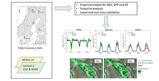
Upscaling Northern Peatland CO2 Fluxes Using Satellite Remote Sensing Data

1
Department of Physical Geography and Ecosystem Science, Lund University, 223 62 Lund, Sweden
2
Centre for Environmental and Climate Science, Lund University, 223 62 Lund, Sweden
3
Finnish Meteorological Institute, Erik Palménin Aukio 1, 00560 Helsinki, Finland
4
Department of Earth Sciences, University of Gothenburg, 405 30 Gothenburg, Sweden
5
Institute for Atmospheric and Earth System Research (INAR)/Physics, University of Helsinki, P.O. Box 64, 00014 Helsinki, Finland
6
Department of Forest Ecology and Management, Swedish University of Agricultural Sciences, 901 83 Umeå, Sweden
7
School of Forest Sciences, University of Eastern Finland, 80101 Joensuu, Finland
*
Author to whom correspondence should be addressed.
Submission received: 15 January 2021 / Revised: 9 February 2021 / Accepted: 20 February 2021 / Published: 23 February 2021
(This article belongs to the Special Issue Remote Sensing of Carbon Fluxes and Stocks)

Abstract

:
Peatlands play an important role in the global carbon cycle as they contain a large soil carbon stock. However, current climate change could potentially shift peatlands from being carbon sinks to carbon sources. Remote sensing methods provide an opportunity to monitor carbon dioxide (CO2) exchange in peatland ecosystems at large scales under these changing conditions. In this study, we developed empirical models of the CO2 balance (net ecosystem exchange, NEE), gross primary production (GPP), and ecosystem respiration (ER) that could be used for upscaling CO2 fluxes with remotely sensed data. Two to three years of eddy covariance (EC) data from five peatlands in Sweden and Finland were compared to modelled NEE, GPP and ER based on vegetation indices from 10 m resolution Sentinel-2 MSI and land surface temperature from 1 km resolution MODIS data. To ensure a precise match between the EC data and the Sentinel-2 observations, a footprint model was applied to derive footprint-weighted daily means of the vegetation indices. Average model parameters for all sites were acquired with a leave-one-out-cross-validation procedure. Both the GPP and the ER models gave high agreement with the EC-derived fluxes (R2 = 0.70 and 0.56, NRMSE = 14% and 15%, respectively). The performance of the NEE model was weaker (average R2 = 0.36 and NRMSE = 13%). Our findings demonstrate that using optical and thermal satellite sensor data is a feasible method for upscaling the GPP and ER of northern boreal peatlands, although further studies are needed to investigate the sources of the unexplained spatial and temporal variation of the CO2 fluxes.

Graphical Abstract

1. Introduction

Peatlands are an important ecosystem for the global carbon cycle, as they cover only 3% of the terrestrial area but contain around 40% of global soil organic carbon [1]. The waterlogged and anoxic conditions in peatlands inhibit the decomposition of plant material, creating a long-term net sink of atmospheric carbon dioxide (CO2) and, consequently, an effective storage of organic carbon [2]. Peatlands assimilate CO2 through photosynthesis (gross primary productivity, GPP) and release it through autotrophic respiration (from vegetation) and heterotrophic respiration (microbial decomposition). The sum of the autotrophic and heterotrophic respiration is the ecosystem respiration (ER). The difference between ER and GPP is the net ecosystem exchange (NEE), which determines whether an ecosystem is a carbon sink or source (excluding gains and losses of carbon through flowing water, biomass removal, or methane fluxes). Pristine peatlands are considered to be net carbon sinks [3], but changing environmental conditions due to global warming or land use change may increase CO2 release and potentially shift peatlands from being carbon sinks to sources [4,5]. For that reason, it is important to estimate peatland CO2 exchange across time and space.
A common method to measure land–atmosphere CO2 exchange at the ecosystem level is the eddy covariance (EC) technique [6]. The EC method provides direct measurements of NEE and nighttime ER, which can be subsequently partitioned into GPP and daytime ER. As the flux partitioning relies on modelling procedures, EC-derived GPP and ER are not considered to be direct measurements but modelled estimates at the ecosystem level.
However, there is only a limited number of EC sites measuring peatland carbon exchange. Peatlands are widespread across the northern latitudes, and to enable the estimation of the CO2 flux from all of these peatlands, it is important to develop remote sensing-based methods for upscaling their CO2 fluxes. The estimation of peatland carbon fluxes with optical remote sensing presents a series of unique challenges due to several characteristic features of peatlands, such as the high proportion of non-vascular plants, high water content, and the effects of microtopographic variations [7]. As a result of their heterogeneity, carbon fluxes may vary widely between peatlands [8,9] and within peatlands [10,11].
Unlike CO2 concentration, CO2 fluxes are not directly detectable by satellites, and hence remote-sensing-derived estimates rely on the relationship between the fluxes and remotely sensed environmental variables. A widely used method to estimate GPP is the light use efficiency (LUE) model by Monteith [12], where GPP is the product of the total photosynthetically active radiation (PAR) incident on the vegetation, the fraction of photosynthetically active radiation absorbed by vegetation (fAPAR), and the conversion efficiency of the absorbed energy (ɛ). Several studies have shown that fAPAR is linearly or near-linearly correlated with spectral vegetation indices like the Normalized Difference Vegetation Index (NDVI) or the Enhanced Vegetation Index (EVI), and therefore a vegetation index often provides a proxy for fAPAR. Although NDVI is widely used in remote sensing-based ecosystem studies, EVI is less sensitive to perturbing factors like atmospheric effects (water vapor and aerosols) and soil reflectance, and more sensitive to variations in vegetation structure [13]. The two-band EVI (EVI2) has been developed to provide similar information as EVI, but it only uses the red and the near infrared (NIR) bands, whereas EVI also uses the blue band [14]. Despite the differences between the spectral indices, both NDVI and EVI have been successfully used to estimate GPP in peatland ecosystems [15,16].
To obtain the full CO2 balance of an ecosystem, both GPP and ER need to be estimated, but as Lees et al. [7] highlight, remote sensing-derived peatland studies have mainly focused on estimating GPP with less consideration of ER. The key challenges are to estimate heterotrophic respiration with high accuracy using remote sensing data [17] and to explain the variability in ER across ecosystems [18]. Despite the challenges, ER has been successfully modelled using satellite land surface temperature (LST) [16,19], and some studies have also included vegetation productivity and soil moisture to improve the ER estimates [18,20,21,22].
The Moderate Resolution Imaging Spectroradiometer (MODIS) instrument mounted on NASA’s Terra and Aqua satellites is widely used to monitor vegetation dynamics, land cover changes, and LST at local and global scales, as it provides both optical and thermal data at a high temporal resolution (1–2 days). However, the heterogeneous character of peatland ecosystems presents a challenge for remote sensing using coarse-resolution (250 m–1 km) sensors like MODIS [23,24]. The MODIS GPP/NPP (MOD17) product at 1 km spatial resolution provides GPP estimates in different biomes [25]. However, the MOD17 product lacks a peatland category in its land cover classification and an estimate of surface moisture, which limits its applicability in peatlands.
The possibility to generate time-series data at high spatial (10–60 m) and temporal resolution (2–3 days at mid-latitudes) using the new Sentinel-2A and 2B satellites with the MultiSpectral Instrument (MSI) presents a new opportunity to map CO2 fluxes in these landscapes. Nevertheless, even with the high frequency of data provided, the presence of clouds and seasonal snow cover cause data gaps of varying length. The TIMESAT v.4 software package provides a flexible yet robust data processing method based on box constrained double logistic functions combined with splines to gap-fill and smooth time series data [26]. The availability of high spatial resolution satellite data also raises the question of how to select a spatial sample of the data that is representative of the EC flux footprint area. Accounting for the flux footprint may be particularly important in peatlands due to their spatial heterogeneity, and can be achieved by using footprint models that can help select the satellite pixels that fall within the EC footprint area [27,28,29].
The potential of remote sensing-based models to predict peatland carbon fluxes has been demonstrated by Schubert et al. [16]. We will expand on this work by using newly available high spatial resolution (10–20 m) optical Sentinel-2 MSI data at five peatland sites across Sweden and Finland, state-of-the-art time-series processing, and footprint modeling to characterize the source area of the CO2 fluxes. Although other carbon fluxes, such as methane (CH4) emissions or dissolved carbon exported by water, also play an important role in peatlands, this study focuses on CO2 fluxes, as these are typically the largest component of carbon exchange in peatlands at annual timescales [5,30].
The aim of this paper is to investigate the feasibility of developing a simple model based on remote sensing data to estimate the CO2 balance (NEE) and its component fluxes (GPP and ER) across different peatlands types at northern latitudes, which could be used for upscaling CO2 fluxes across northern boreal peatlands. As part of this aim, we investigate a) with what accuracy we can model the NEE flux and its components using a single parameter set for our five sites, compared to using individual parameter sets for each site, and b) with what accuracy directly modeled NEE differs from the sum of modelled GPP and ER.

2. Materials and Methods
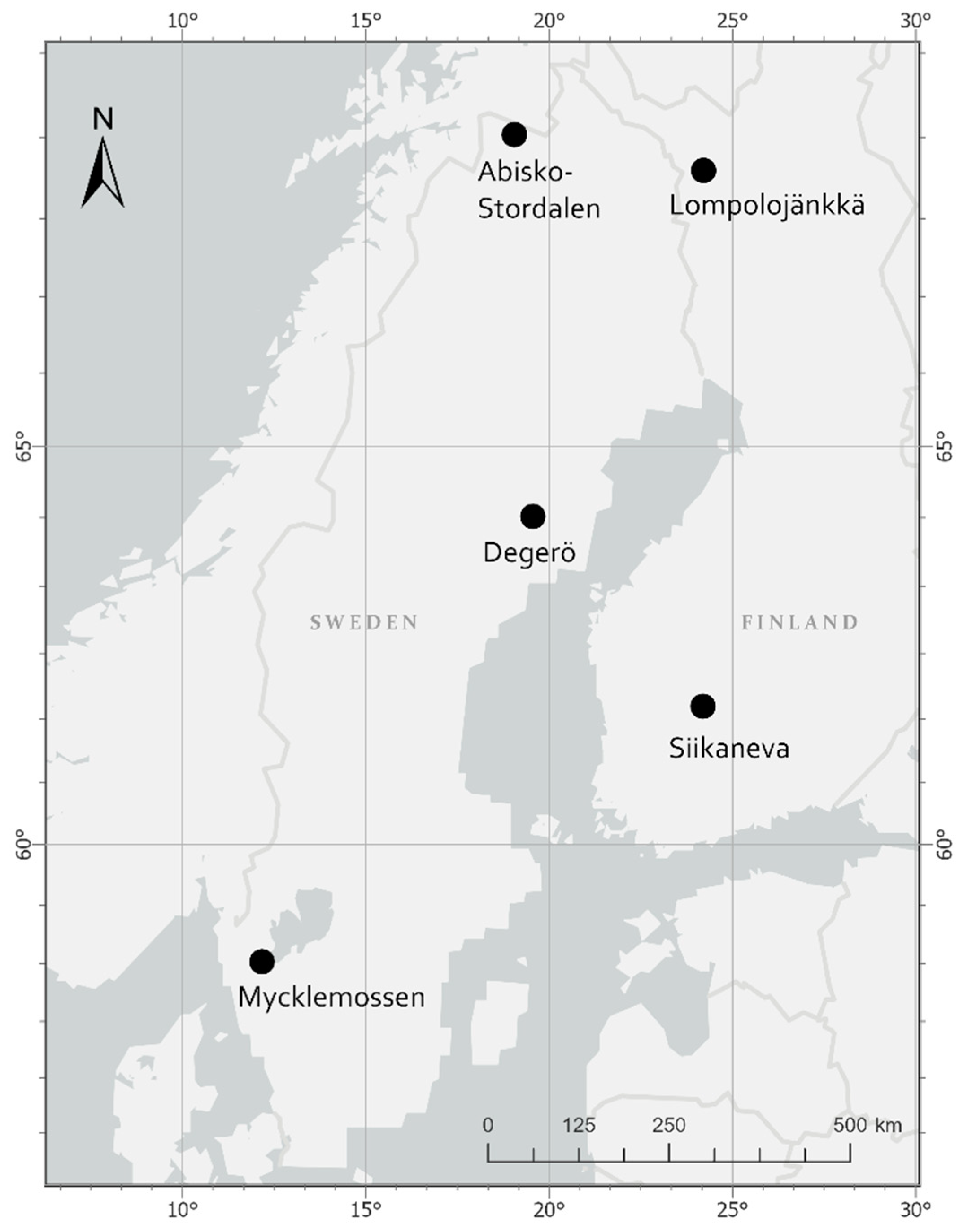
2.1. Study Sites

The study includes five Nordic peatland sites located in Sweden and Finland: Abisko-Stordalen, Degerö, Mycklemossen, Siikaneva, and Lompolojänkkä (Figure 1, Table 1). Mycklemossen is part of the SITES (Swedish Infrastructure for Ecosystem Science) infrastructure, whereas the other sites belong to the ICOS (Integrated Carbon Observation System) infrastructure. The sites were selected to cover peatlands exposed to different climatic conditions (hemi-boreal, boreal, and subarctic), at northern latitudes from 58°N to 68°N. Four of the sites are fens, and one, Abisko-Stordalen, is classified as a bog, although it also contains areas of fen. The study period spanned between 2017 and 2019, though data availability varied among the sites. Further information on each site can be found in Table 1.

2.2. Eddy Covariance Flux Data

The eddy covariance (EC) measurement system at Lompolojänkkä included a USA-1 three-dimensional sonic anemometer (METEK GmbH, Elmshorn, Germany) and a closed-path LI-7000 CO2/H2O infrared gas analyzer (LI-COR, Inc., Lincoln, NE, USA). At Siikaneva and Mycklemossen a USA-1 anemometer was used with an LI-7200 (LI-COR Inc., USA) gas analyzer. At Degerö, a 1012R3 Solent (Gill Instruments, Lymington, UK) anemometer was used with an IRGA LI-6262 (LI-COR Inc., USA) gas analyzer and the Abisko-Stordalen site used a uSonic-3 Class A (METEK GmbH, Germany) anemometer with an LI-7200 gas analyzer.
From the high frequency (10 Hz) EC data, 30-min CO2 fluxes were derived taking into account the corrections following [35]. At the ICOS Sweden sites, the open source EddyPro® Eddy Covariance Processing Software, version 6.0 (LI-COR Biosciences, Lincoln, NE, USA), was used following the ICOS protocol for data processing [36,37]. The processing procedures at Lompolojänkkä and Siikaneva have been presented in Aurela et al. [31] and Korrensalo et al. [10], respectively. More details on the data processing at Mycklemossen are given in the Supplementary Materials. The processed EC fluxes were partitioned into GPP and ER and gap-filled using standard methods with an exponential temperature response for respiration [38] and a saturating light response for GPP [39].
Daily averages of the fluxes were calculated from the gap-filled 30-min CO2 flux data acquired from the sites and the time series were smoothed using a spline function in TIMESAT (see Table S1 for the spline parameters). We applied the same spline parameters as used for the LST data (see Section 2.3) to reduce the high-frequency (daily) variations in the flux data that could not be captured by the remote-sensing data due to its coarser temporal resolution. The smoothing of the CO2 flux data did not have a substantial effect on the seasonal shape of the fluxes or the annual NEE balance (see Section 3.3).

2.3. Remote Sensing Data

The models to estimate GPP, ER, and NEE were driven by vegetation indices based on Sentinel-2-retrieved data along with LST data from MODIS.
Sentinel-2 MSI images covering an area of 100 by 100 km at each site from 2017–2019 were downloaded from the European Space Agency (ESA) Copernicus Sentinels Scientific Data Hub. The Sen2Cor processor (version 2.8.0) was used to perform atmospheric corrections and obtain land surface reflectance and scene classification [40]. The vegetation index EVI2 [14], with a spatial resolution of 10 m, was calculated using red (RED) and near-infrared (NIR) reflectances:
EVI 2 = 2.5 N I R R E D N I R + 2.4 R E D + 1   .
A vegetation index related to water content, the Normalized Difference Water Index (NDWI) [41], was calculated using 20 m resolution NIR and short-wave infrared (SWIR) bands:
NDWI = N I R S W I R N I R + S W I R   .
Both data sets were gap-filled and smoothed pixel-wise using a spline function in TIMESAT to produce daily values (Table S1).
In order to select the NDWI and EVI2 pixels that fell within the flux source area, the EC flux footprint was estimated at each site with the Flux Footprint Prediction (FFP) model [28]. The model was driven by 30-min micrometeorological data (collected as part of the EC measurements, see Section 2.2) to produce daily footprint climatologies. The footprint climatologies were used to calculate weighted daily means of the EVI2 and NDWI within 80% of the footprint area. Furthermore, the time-series of the mean daily EVI2 and NDWI were both scaled so that the index value was 0 when GPP was 0. This procedure enabled the combination and comparison of data from all the study sites, as the base values of the indices were usually not equal to zero and varied from site to site.
As NDWI expresses the effect of soil hydrology on the vegetation, NDWI was used to calculate a water scalar (Ws), following Xiao et al. [42]. The Ws represented the variations of moisture conditions interannually and between the sites. Other scalars that were tested are presented in Table S2. A simple version of the water scalar by Xiao et al. [43] was selected for the further analysis:
W s = 1 + NDWI max ,
where NDWImax is the 99th percentile of NDWI during the growing season. During the dormant season, Ws was set to 1. The growing season was defined for each site and year based on when the daily mean air temperature (Tair) exceeded +5 °C for seven consecutive days [9].
The LST data was acquired from the MODIS instruments mounted on the Terra and Aqua satellites. The MODIS LST products (MOD11A1, MYD11A1) include daily daytime and nighttime LST at 1 km spatial resolution, providing a maximum of four LST measurements per day. LST data were smoothed and gap-filled in the same way as the flux data and spectral indices using TIMESAT (Table S1). Due to the coarse resolution of the MODIS data, the footprint model was not used with these data, but we extracted data from one pixel where the EC tower and the peak of the flux footprint was located at each site. Daytime LST was used in the rest of the analysis due to the higher number of high quality images and a better fit with ground LST measurements that were available from some of the sites (R2 = 0.85, RMSE = 5.3 °C for Degerö 2017–2019 and R2 = 0.75, RMSE = 6.1 °C for Abisko-Stordalen 2017–2019).

2.4. Empirical Regression Models for GPP, ER, and NEE

The GPP model structure was based on previous work by Schubert et al. (2010), where EVI, LST, and photosynthetic photon flux density (PPFD) were used as regression model inputs. In this study, we investigated how satellite-derived EVI2, LST, and Ws along with site-measured environmental variables (Tair, PPFD, water table depth (WTD) and annual precipitation) were related with GPP time-series data. Based on the goodness-of-fit of the regressions, EVI2, Ws, and daytime LST were chosen as input variables into the GPP model. The derived linear regression model for estimating GPP at all the sites simultaneously can be described as:
GPP = a × EVI 2 × W s × LST .
Because of the abovementioned scaling of EVI2 and NDWI, it was possible to force the regression line through the origin, which is a physically reasonable way to estimate GPP. Equation (4) can be regarded as an empirical variation of the LUE model, where the parameter a, Ws, and LST jointly function as a proxy for PAR and the light use efficiency coefficient. Since photosynthesis does not take place in cold temperatures, only data when LST was above 0 °C were used to determine the model parameter a.
Ecosystem respiration (ER) was also modelled using an empirical model. Three existing models were tested: Lloyd and Taylor [44] (Equation (5)), Heskel et al. [45] (Equation (6)), and Gao et al. [46] (Equation (7)), who added the dependence on GPP to Lloyd and Taylor’s model:
ER = R r e f e E 0 ( 1 T r e f T 0 1 T + 273.15 T 0 ) ,
lnER=a+bT+c T 2 ,
ER = a × GPP + R r e f × e E 0 ( 1 T r e f T 0 1 T + 273.15 T 0 ) ,
where Tref = reference temperature (set to 10 °C); T = daytime LST; T0 = –46.02 °C (value taken from Lloyd and Taylor [44]); GPP = modelled GPP; and Rref, E0, a, b, and c are parameters to be estimated. To model ER, we started by testing the three models (Equations (5)–(7)) at each of the sites separately, for all available years, in order to find the best model (see results in Table S3). We also tested multiplying each model by an EVI2 scalar (formulated in the same way as Ws) or the Ws scalar (Table S3). The Gao et al. [46] model (Equation (7)) provided the best fit. Including vegetation productivity in the ER model improved the fit, because it helped better capture the magnitude and timing of the peak growing season ER. We tested modelling ER separately during the growing and dormant seasons, but it yielded no or only minor improvements in the goodness-of-fit.
Since Equation (7) is sensitive to possible errors in the modelled GPP as an input, EVI2 was used as a proxy for modelled GPP to reduce the uncertainties in the modelled ER (Equation (8)). Equation (8) was the ER model used in the rest of the analysis:
ER = a × EVI 2 + R r e f × e E 0 ( 1 T r e f T 0 1 T + 273.15 T 0 ) .
We compared two methods for modelling NEE, where NEE = ER - GPP. We followed the sign convention that NEE is negative when the ecosystem is a carbon sink (GPP > ER) and NEE is positive when the ecosystem is a carbon source (ER > GPP). NEE was estimated 1) by subtracting the modelled GPP (Equation (4)) from the modelled ER (Equations (2) and (8)) by fitting a non-linear regression model that included the GPP and ER components (Equation (9)) to the EC NEE measurements:
NEE = b 1 × EVI 2 + R r e f × e E 0 ( 1 T r e f T 0 1 T + 273.15 T 0 ) b 2 × EVI 2 × W s × LST .
In addition to these two NEE models, we also tested a third, purely empirical, NEE model based on multiple linear regression. EVI2, NDWI, LST, PPFD, WTD, and Ws were fitted as predictor variables against EC NEE measurements. However, this approach was not selected for further analysis, because PPFD and WTD were not available at all sites and years, and it did not provide a consistent improvement compared to the non-linear NEE model (Equation (9)). See Supplementary Materials for more details.
In the first stage of the analysis, the free parameters for the GPP, ER, and NEE models were estimated separately for each site using all the available years of flux data (Table S4), and in the second stage, the parameters were estimated for all the sites together (Tables S5–S7). To obtain one parameter set for all the sites, leave-one-out cross-validation (LOOCV) was used, i.e., the models were fitted using data from all the sites except for one site-year, which was used to validate the fitted models. After all the LOOCV runs, the mean model parameter values were applied to all the sites.

3. Results

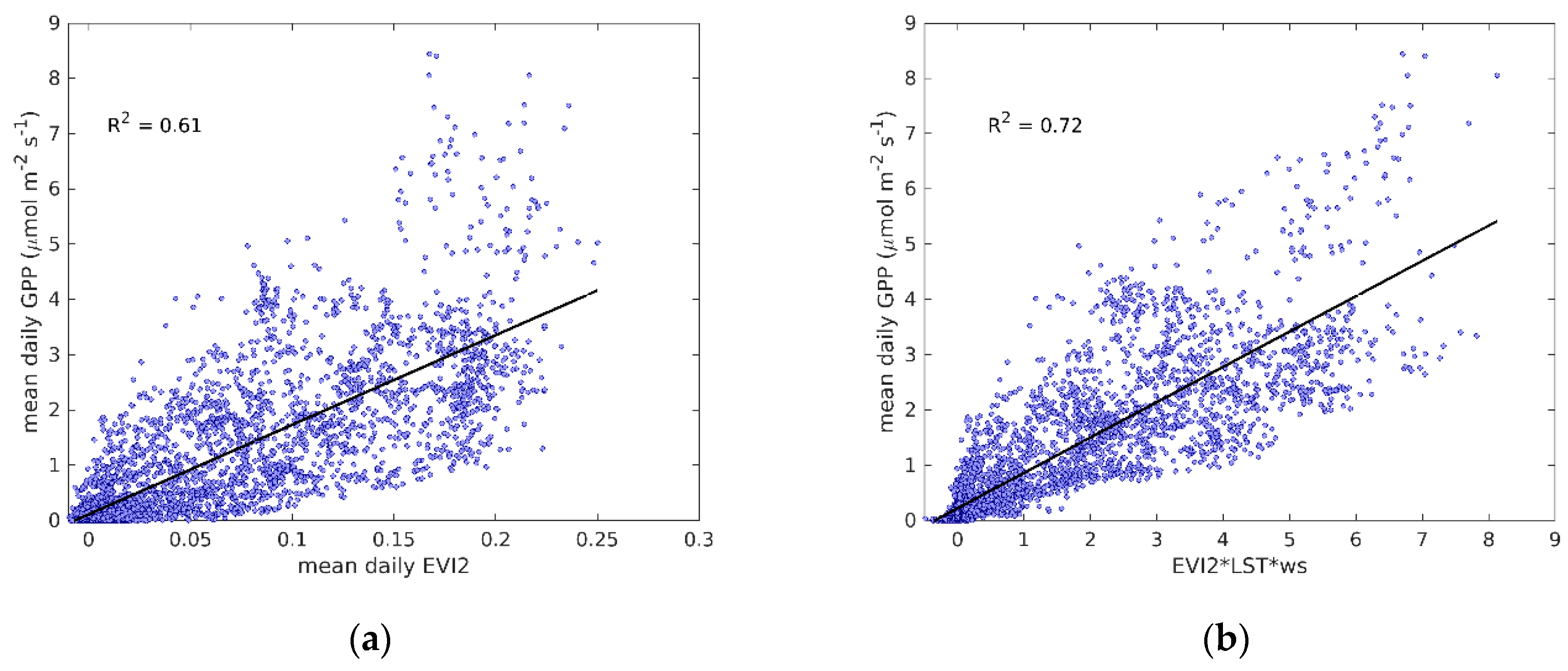
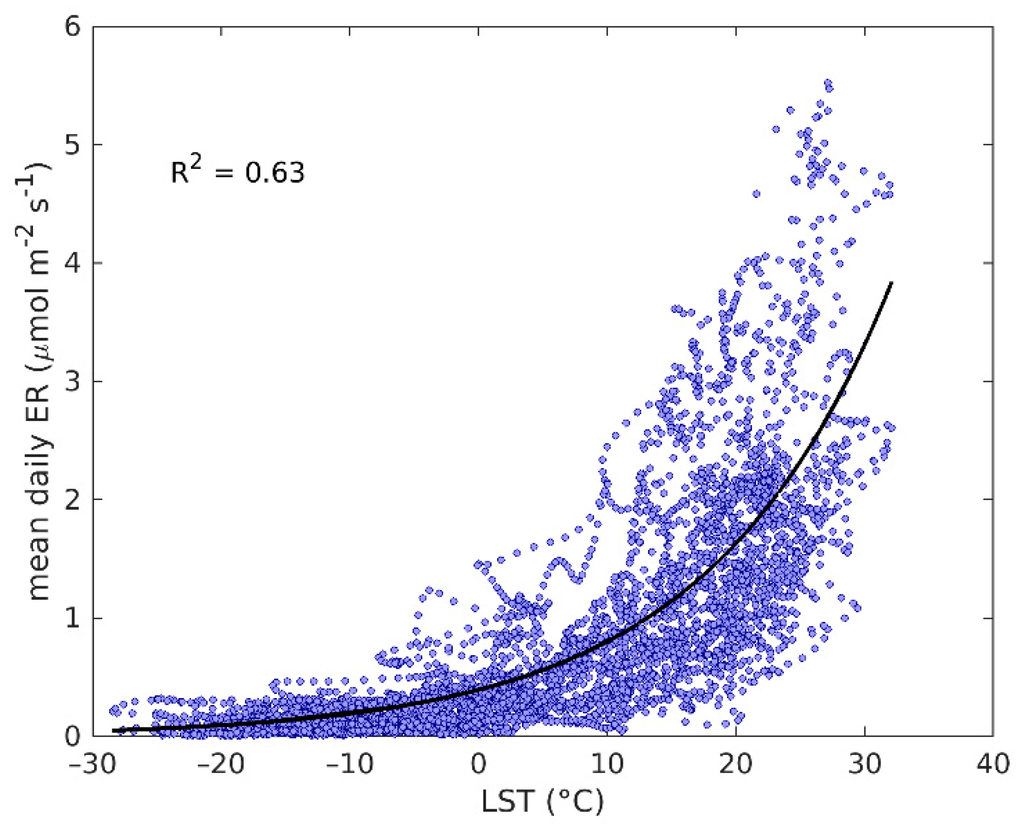
3.1. Relationships between GPP, ER and Remote Sensing Variables

Daily mean EVI2 from Sentinel-2 showed a clear relationship with flux tower derived GPP, R2 = 0.61 for all sites and years together (Figure 2a). Stronger relationships were found when studying each site and year separately, and differences in the relationship between GPP and EVI2 during the spring and autumn were also clearer at some sites (Figure S1a). These results indicate that it would be possible to use different regression models for the spring green-up and the autumn senescence, as the relationships seemed to be logarithmic and exponential, respectively, instead of linear. However, since it was not possible to define general functional relationships that could be used across all sites, we used linear relationships between EVI2 and GPP. In addition to EVI2, we used LST and Ws as proxies for the environmental variables controlling GPP, reducing the tendency to underestimate high GPP and increasing the strength of the relationship (R2 = 0.72, Figure 2b).
There was also a strong exponential relationship between ER and LST, R2 = 0.63 at all sites, and years together (Figure 3). Similarly to the relationship between EVI2 and GPP, some sites showed clear seasonal variation in the ER–LST relationship between the spring and autumn (Figure S1b).

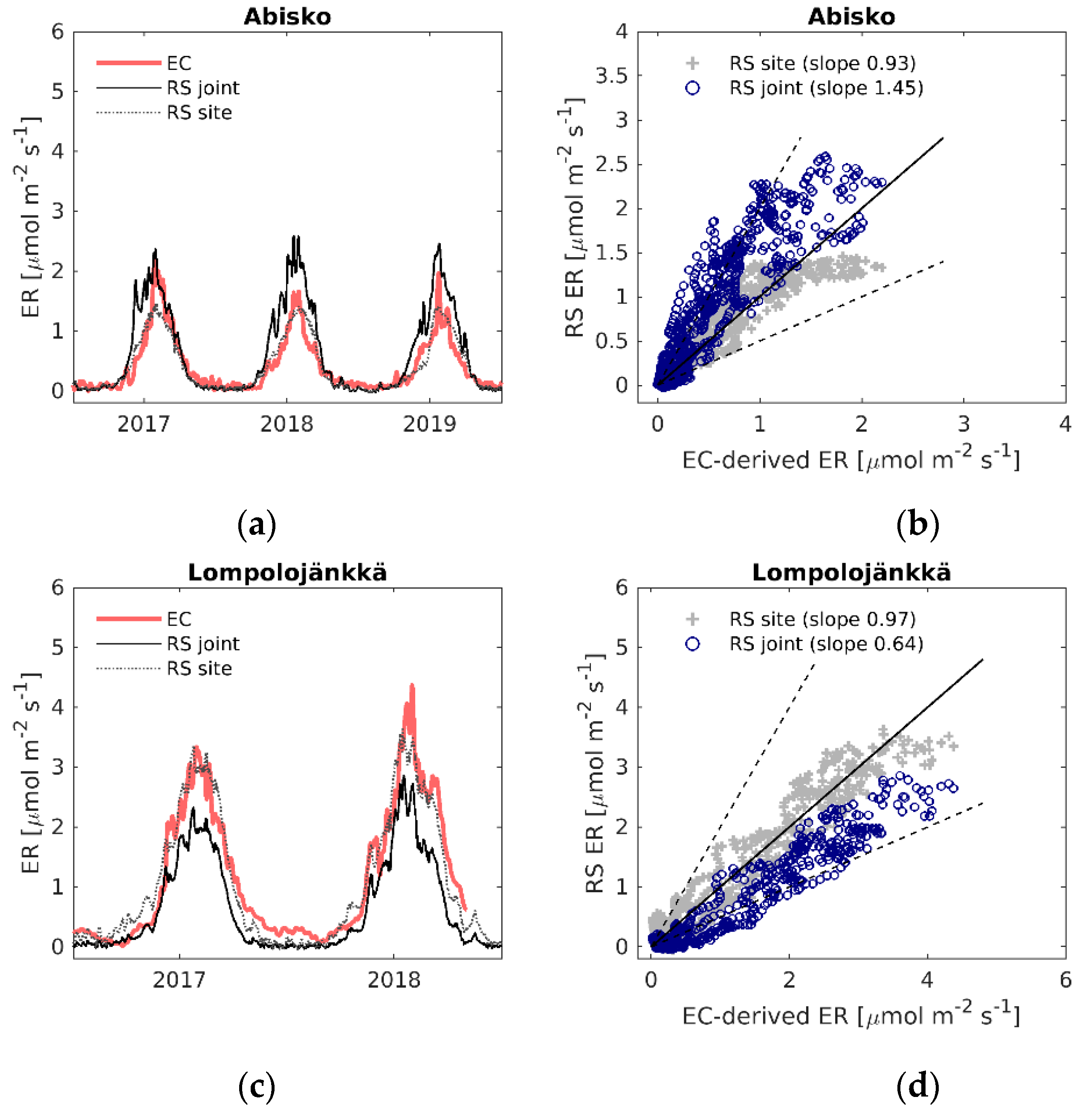
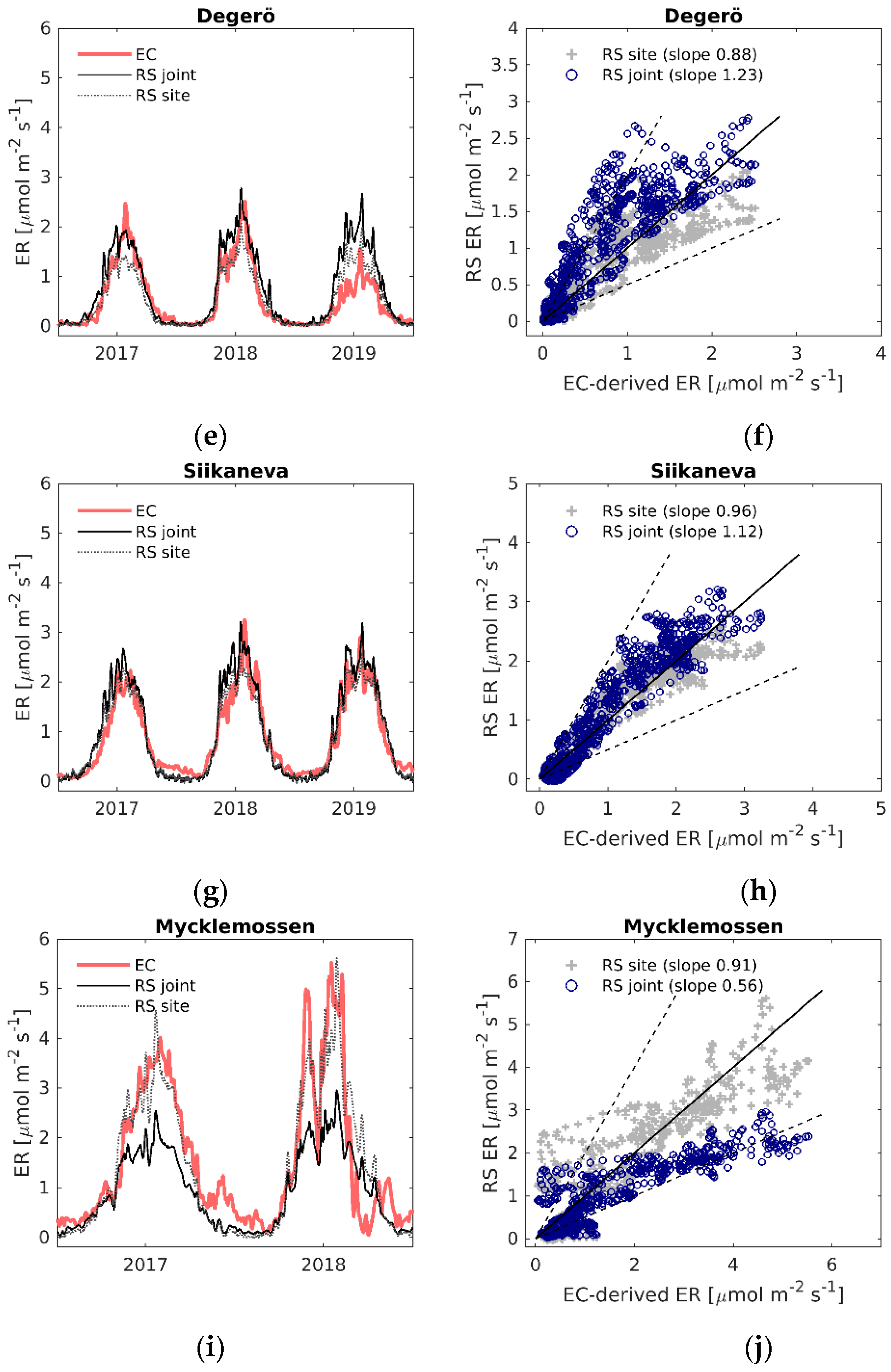
3.2. GPP and ER Models
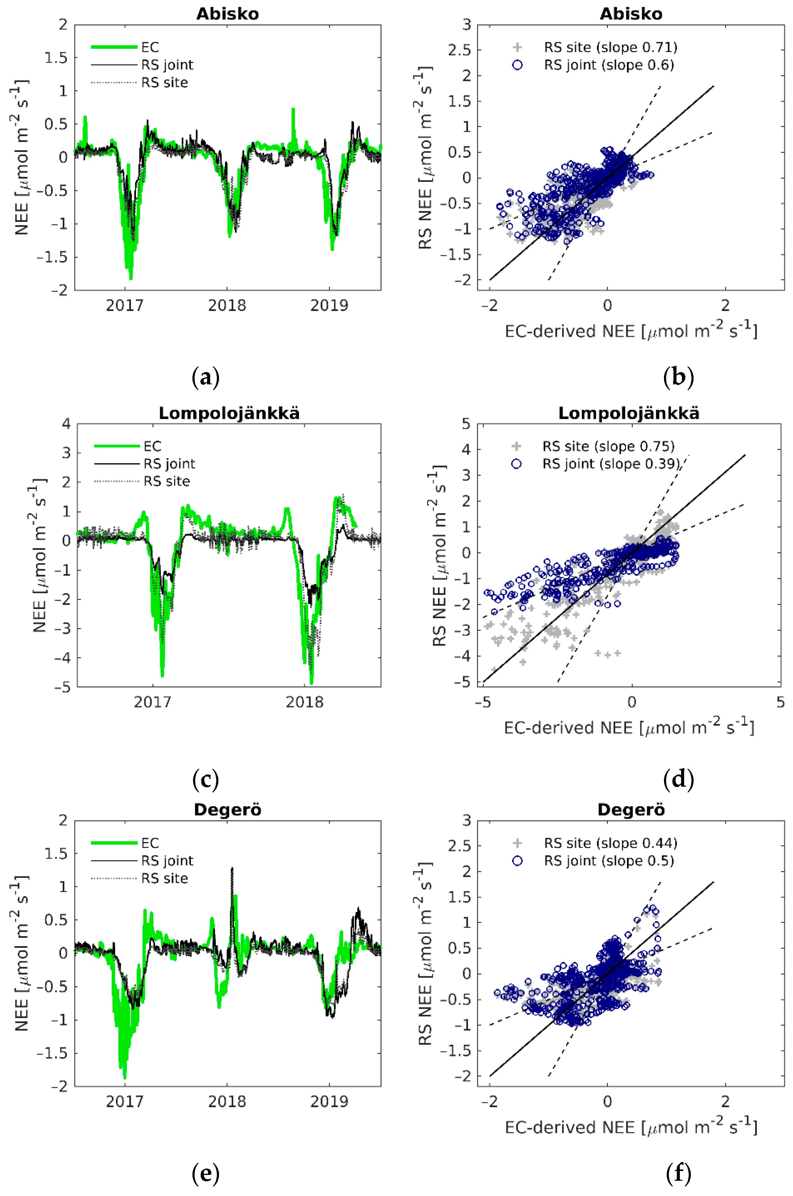
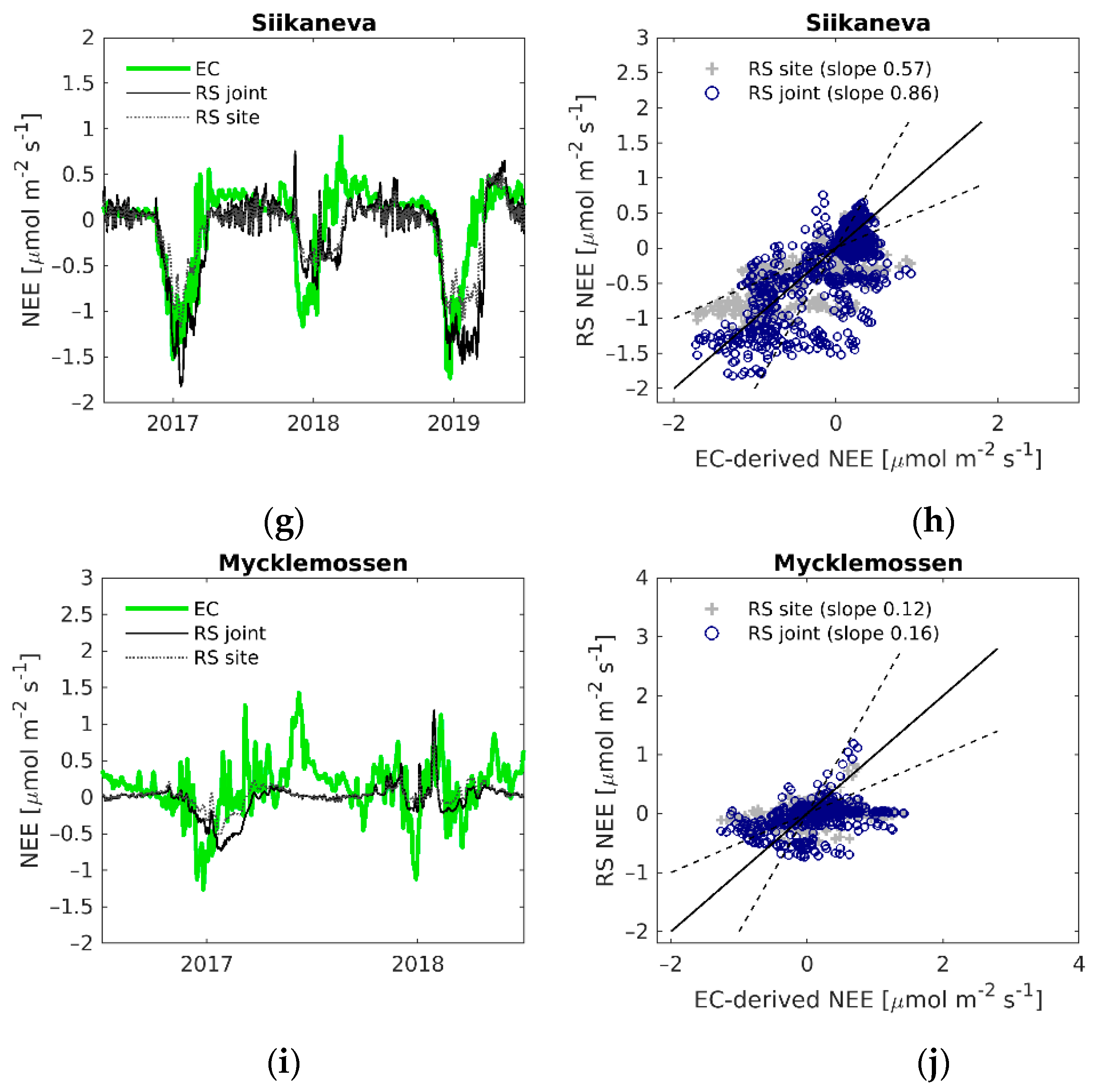
For GPP, the LOOCV parameterized linear regression model (Equation (4)), with the average coefficient a = 0.70 (Table S5), resulted in high agreement between modelled and EC-derived GPP at all the sites (R2 = 0.54–0.78, RMSE = 0.42–0.98 µmol m−2 s−1, Table 2). Based on the normalized root mean square error (NRMSE), the best fit was found at Abisko-Stordalen, where the error was 10% of the range of the EC-derived GPP, whereas the worst fit was found at Mycklemossen (NRMSE = 20%).
For ER, the agreement between the LOOCV parameterized model fit (Equation (8), see Table S6 for parameters) and the EC-derived ER differed between the sites more than the GPP model fit: R2 varied between 0.23–0.85, and RMSE was between 0.31–0.98 µmol m−2 s−1 (Table 2). The NRMSE of the ER model fit was similar to that of the GPP model, varying from 10% to 20%. The ER model performed best at Siikaneva, whereas the weakest relationships were found at Abisko-Stordalen and Mycklemossen. Using site-specific parameters (Table S4), the model NRMSE was reduced to between 7–12% of the flux range for both the GPP and ER estimates (Table 3).
The time-series of the modelled and EC-derived fluxes (Figure 4 for GPP, Figure 5 for ER) show that the LOOCV parameterized models are able to capture the seasonal variation of the fluxes. However, some noticeable under- and overestimations of GPP and ER occur during the peak of the growing season. The LOOCV parameterized ER model also tended to underestimate the wintertime ER fluxes, especially at Lompolojänkkä and Mycklemossen (Figure 5c,i). Using the models with site-specific parameters helped better capture the peak of the fluxes, with less improvement in the general seasonal shape. The time-series of the LOOCV parameterized modelled GPP for Mycklemossen and Lompolojänkkä show a delayed start of the growing season compared to the EC-derived GPP (Figure 4c,i). Similar effects can be observed at Abisko-Stordalen in 2019 and Degerö in 2017 (Figure 4a,e). As noted above, the LOOCV parameterized GPP and ER models performed poorly at Mycklemossen, and Figure 4i and Figure 5i show that both fluxes were significantly underestimated at this site. Several environmental variables related to GPP and ER were tested in order to find a scaling factor that could help to improve the ability of the models to capture the growing season peak of the fluxes (Table S2), but no strong correlations were found. The NDWI-based water scalar (Ws) was selected for GPP modelling, as it improved the agreement between modelled and EC-derived GPP at Lompolojänkkä and Mycklemossen. The influence of this variable was small at the other sites, and it did not improve the accuracy of modelled ER (Table S3).

3.3. NEE Models

Out of the two NEE models, the non-linear regression model (Equation (9)) generally performed better than calculating the difference of modelled GPP (Equation (4)) and modelled ER (Equation (8)) when compared against EC-measured NEE (see Table 2 for LOOCV parameterized model prediction estimates and Table 3 for site-specific estimates). The site-specific model parameters (Table S4) gave higher agreement than the average parameters from the LOOCV (Table S7). Overall, the performance of the NEE models was weaker than the GPP and ER models, although at Abisko-Stordalen and Lompolojänkkä the non-linear regression NEE model with site-specific parameters gave similar agreement to that of GPP and ER, R2 > 0.70, and NRMSE around 9% of the range of measured NEE (Table 3).
The time-series of modelled and measured NEE show that modelled NEE corresponds fairly well to measured NEE, and the seasonal shape of NEE was captured at most of the sites and years (Figure 6). However, the models have difficulties capturing the growing season peak, as seen for instance at Abisko-Stordalen in 2017 (Figure 6a), and the periods of positive NEE (when ER is higher than GPP) at the start and end of the growing season. The latter can be seen clearly at Lompolojänkkä in both years (Figure 6c). The poor performance of the GPP and ER models at Mycklemossen are also shown in the NEE time-series, where the modelled NEE corresponds weakly to the measured NEE (Figure 6i).
The comparison of the annual cumulative modelled NEE and measured NEE (Figure 7) emphasizes the importance of accurate flux modelling, as small over- or underestimations, not only during the peak growing season, but during the whole year, can result in a significant difference in the annual CO2 budget. For example, the NEE models at Abisko-Stordalen in 2017 underestimated the NEE growing season peak equally (Figure 6a), but result in very different annual accumulation of CO2. The model with the site-specific parameters suggests that the site is a CO2 sink, whilst the model with the average parameters suggests that the CO2 budget is close to zero (Figure 7). Table S8 shows that the modelled annual NEE differed largely from the measured annual NEE at most of the sites and years. The model was able to estimate the annual NEE accurately (maximum 3% difference to the measured NEE) at Abisko-Stordalen 2017 (site-specific estimate), Abisko-Stordalen 2018 (predicted with joint parameters), and Siikaneva 2017 (site-specific estimate). The linear regression model with site-specific parameters performed slightly better than the model with jointly estimated parameters at eight out of 13 site-years.

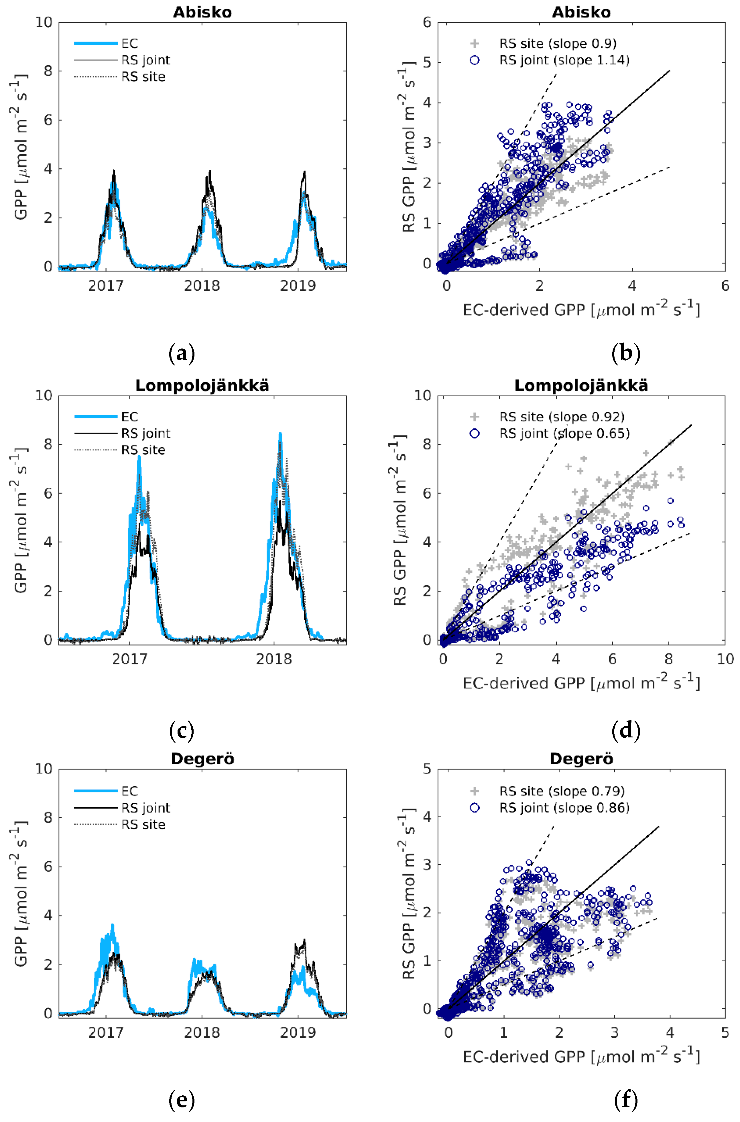
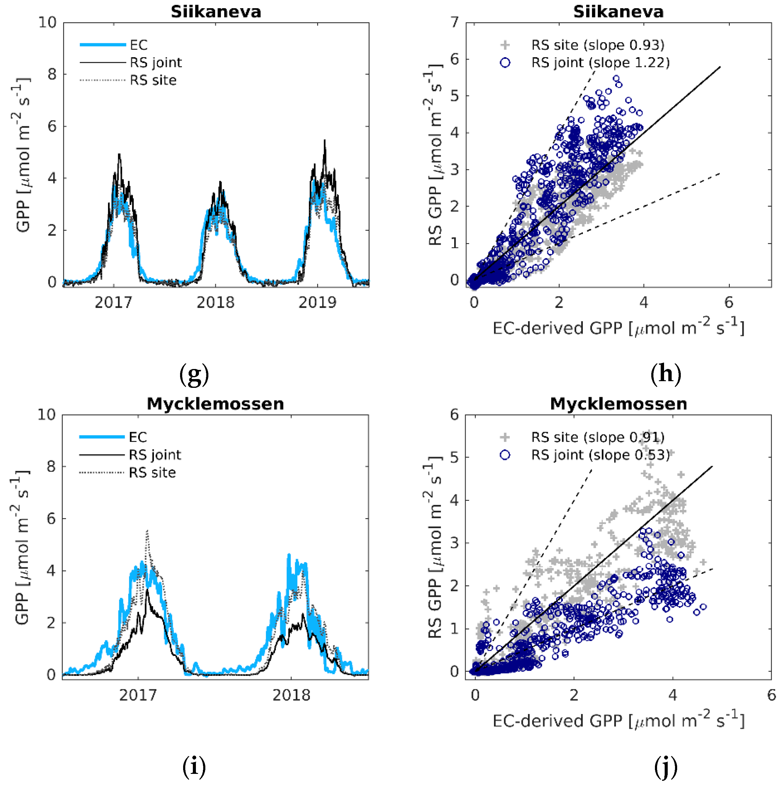
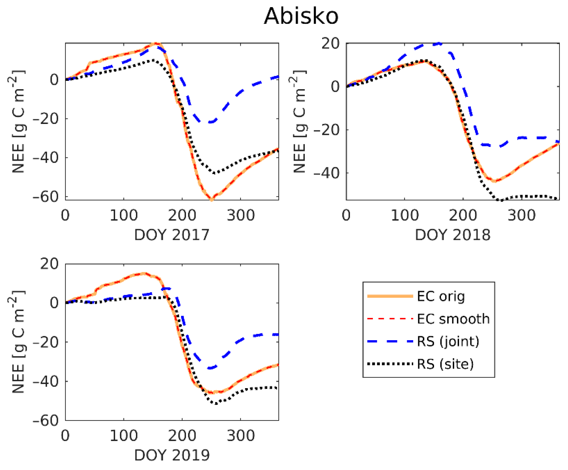
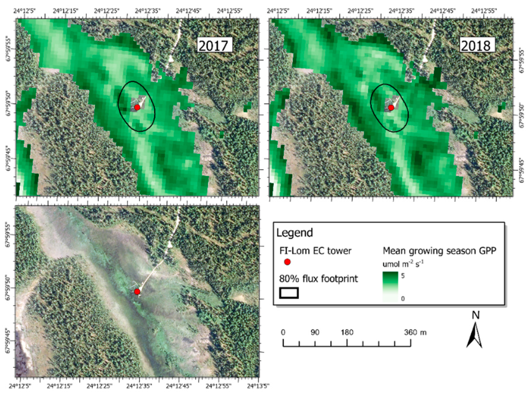
3.4. Upscaling GPP to the Peatland Scale

In order to demonstrate the applicability of the simple regression model with high resolution satellite data for upscaling, we applied the GPP model (Section 3.2, Equation (4)) with the average parameters from the LOOCV (Table S5) to Sentinel-2 data for the Lompolojänkkä site (Figure 8). We selected Sentinel-2 pixels for upscaling based on the wetland land cover classification in Finland (SYKE, 2018), so that only pixels in the class “open peatbog” were used. Figure 8 shows the estimated average GPP during the growing season in 2017 and 2018. GPP varies from 1 up to 5 µmol m-2 s-1 within the flux footprint area, and similar spatial variation can be seen also beyond the flux footprints in both years.

4. Discussion

The results of this study showed that purely remote sensing (RS) derived data can be used in regression models to estimate seasonal CO2 uptake and release from northern peatlands. The product of EVI2, LST, and an NDWI-based water scalar (Ws) explained a large proportion of the variability in GPP at all the sites. In addition, ER was strongly related to daytime LST, and based on these findings, NEE could be estimated from LST in combination with EVI2 and Ws. However, the accuracy of the estimated fluxes was inconsistent across the sites and years. It should be noted that the EC-derived fluxes vary at a high frequency that satellite remote sensing data cannot reproduce. Smoothing the time-series of EC-derived NEE, ER and GPP made them more comparable to the remote sensing data. Nevertheless, the RS models rely on LST to capture the daily variations in the fluxes, because LST is the only remote sensing dataset that varies significantly at a daily scale, whereas EVI2 and NDWI vary more slowly over the growing season. This means that short-term variability can only be captured at a coarse spatial scale.
Some sites showed clear variations in the ER-LST and the GPP-EVI2 relationships between the spring green-up phase and the senescence phase, suggesting that each phase should be modelled separately. However, during initial testing, we found that separating the CO2 fluxes between different seasonal stages was not straightforward. A simple split of a flux time series between the green up phase and the senescence phase can cause problems with modelling the peak season accurately, and therefore we decided to model the whole year at once. Further analyses may reveal solutions to this challenge.
The linear regression model for GPP that we developed is an empirical variation of the formal LUE model by Monteith [12]. LUE models usually include PAR. In this study, PAR was not included in the GPP model, as it showed very weak relationships with daily GPP at all the sites. Instead, the regression parameter, the water scalar Ws, and LST jointly provided a proxy for PAR and the LUE term, but these factors might not be sufficient to explain all spatial and temporal variations of the photosynthetic efficiency within a peatland ecosystem. Alternative ways to estimate the LUE coefficient using remote sensing methods, such as the photochemical reflectance index (PRI) [47], may solve this issue [48]. Unfortunately, the wavelength bands to calculate PRI are not available from Sentinel-2. Another remote sensing-derived variable that can be used to estimate GPP is solar induced fluorescence (SIF) [49], which will be operational at the ecosystem scale in future from the forthcoming Fluorescence Explorer (FLEX) satellite mission by ESA.
LST explained ER well at all sites. Including productivity in the ER model (using EVI2 or modelled GPP) improved the model fit compared to the original Lloyd and Taylor [44] model. Gao et al. [46] argue that the Lloyd and Taylor equation represents heterotrophic respiration, and including GPP is a way of including information related to autotrophic respiration in the estimate. It has been shown that ER is tightly linked to vegetation productivity [50,51,52], and a productivity or greenness index has also been used in remote sensing models of ER before [18]. Our results demonstrate that using EVI2 instead of modelled GPP (as proposed by Gao et al. [46]) gives similar model accuracy whilst also making the model simpler and more robust. However, the LST and EVI2 based model might be less suitable to estimate ER in winter, since low soil surface temperatures and vegetation productivity predict low fluxes, while higher temperatures in deeper layers of peat enable decomposition to continue [53]. Wintertime ER can be an important part of the annual CO2 balance in northern peatlands that is possibly underestimated by surface temperature driven models [54]. Separate ER model fits for the whole dormant season did not improve ER estimates, but future work could investigate this using separate model fits specifically during periods with snow cover (similar to Jägermeyr et al. [18]) or using LST as input to model peat temperature during the winter.
Of the two types of NEE models tested, the non-linear regression model performed generally better than the model that was calculated by subtracting GPP from ER. This might be due to error propagation [16]. It is challenging to model NEE directly, as it is the difference between two large fluxes driven by separate processes with different seasonal dynamics. Although the largest under- or overestimations were found during the peak growing season, our results indicate that small differences during the whole year greatly influence the annual NEE as well.
The modelling results showed that site-specific parameterization usually gave higher agreement with the EC fluxes than the average parameters from the LOOCV runs. However, for upscaling purposes, an average parameter set is more applicable than parameters that are strictly associated with one site. To reduce the importance of the regression parameters, other variables, that are able to explain the differences between the years within a site and also between the sites, could be included in the models. We tested several variables to scale GPP and ER in order to capture differences in the growing season fluxes between the sites, but none of them were strongly related to peak GPP or ER.
The NDWI-based water scalar was selected for GPP modelling, as in general, WTD is one of the most important variables regulating the function of peatland ecosystems [55]. Measures of soil moisture availability or precipitation have also been used previously to model ER [21], but our initial tests found that including the NDWI or Ws in the ER model did not improve the fit. NDWI is a spectral index expressing the influence of soil moisture on the vegetation rather than an actual soil moisture index, and it does not fully capture the seasonal variations in water table depth within a site (see Figure S2) or differences between sites (Table S2). Further work is needed to find remote sensing variables better able to capture variations in water table depth or soil moisture at peatland sites; for this purpose, hyperspectral and synthetic aperture radar data have shown promising results [56,57]. Alternatively, the CO2 flux modelling could be combined with hydrological modelling to further investigate how, for example, water table depth changes or snow melt timing affect the fluxes. For instance, Huang et al. [58] assimilated regional soil moisture network data, remote sensing data, and high-resolution land surface parameters to develop an empirical soil moisture model.
Our modelling approach investigated to what extent a single set of parameters is sufficient to upscale the CO2 fluxes from a variety of northern peatlands. Future work could examine which improvements may be gained by modelling the fluxes of different peatland types (i.e., bogs and fens) separately. For example, our ER model with average parameters performed worst at Abisko-Stordalen, the only ombrotrophic bog in our study. Similarly, Kross et al. [15] found differences in the relationships between remote sensing vegetation indices and peatland CO2 fluxes depending on the presence of trees and peatland type. Bogs and fens have also been shown to respond differently to changes in water table and air temperature [59,60] due to their contrasting vegetation assemblages.
Improving the GPP and ER estimations separately would also improve the NEE model estimation. An alternative approach to estimate NEE could be a multivariate linear regression model including all remote sensing and environmental variables that are available at a site. This method lacks the more mechanistic scheme that our NEE model (Equation (9)) has, but the advantage is the high number of free parameters that makes the model adjustable. This method could be used to estimate NEE at an individual site that differs from other sites in its characteristics, e.g., at Mycklemossen, which is more light-dominated than the other sites in our study (Figure S3).
During the summer of 2018, northwestern Europe experienced a severe drought, which increased air temperatures, lowered WTD, and thus reduced the CO2 uptake at several northern peatlands [61]. Rinne et al. [61] found that the 2018 drought did not affect all peatlands equally, as local hydrological features can make a peatland less sensitive to climatic variations, as was the case at Lompolojänkkä. Similarly, compared to 2017 and/or 2019, the EC-derived NEE we present was lower in 2018 at Abisko-Stordalen, Degerö and Siikaneva, but not at Lompolojänkkä. The decrease in NEE at these sites mainly originated from reduced GPP, although increased ER in 2018 was observed at Siikaneva. Lower GPP and ER were found at Degerö in 2019, which was also a dry year at that site. However, the dry conditions in 2019 did not influence the spectral properties of the vegetation, as the EVI2 in 2019 is at the same level as in 2017, which causes the mismatch between modelled and measured GPP. It is also possible the 2018 drought has a legacy effect in 2019, i.e., the vegetation did not fully recover from the drought in the previous year, and therefore both GPP and ER were lowin 2019 at Degerö. Mycklemossen experienced droughts both in 2017 and 2018 [61], and was also the southern-most (i.e., warmest and most light-dominated) site in the study, which may partly explain why our models with the average parameters performed poorest here. Overall, with only two or three years of data, it is difficult to draw strong conclusions about the temporal variations of the fluxes, especially if a severe drought has been experienced at a site.
Despite the limitations discussed above, our findings suggest that using satellite data in regression models is a simple yet powerful tool for modelling and upscaling GPP and ER. Due to its high spatial resolution, Sentinel-2 data has great potential to upscale GPP from the flux footprint to larger areas. The main input of the ER model, MODIS LST, has a coarse spatial resolution (1 km), which makes it less feasible to study heterogeneous ecosystems like peatlands. However, in this study, the MODIS LST was chosen over the 30 m resolution thermal Landsat data because of the higher temporal resolution and because it is a readily available LST product. To improve the spatial resolution of MODIS data, an appropriate downscaling procedure from MODIS reflectance to the Landsat 30 m resolution could be used [62]. Preserving the high temporal resolution while increasing the spatial resolution would enable the mapping of the spatial variation of LST within a peatland and within the flux tower footprint and may lead to improved ER and GPP models.

5. Conclusions

In this study, we demonstrated that regression models driven by remote sensing-derived data can be used to estimate CO2 fluxes in northern peatlands (Abisko-Stordalen, 68°N; Lompolojänkkä, 68°N; Degerö, 64°N; Siikaneva, 62°N; Mycklemossen, 58°N) at relatively high accuracy. A strong relationship was found between GPP and the product of Sentinel-2 EVI2, Sentinel-2-derived water scalar (Ws), and daytime LST from MODIS. ER was strongly related to MODIS LST, and including EVI2 as a proxy for GPP improved the agreement with eddy covariance-derived ER. NEE was successfully explained by MODIS LST in combination with Sentinel-2 EVI2 and Ws at Abisko-Stordalen and Lompolojänkkä. At other sites, however, the relationship between modelled NEE and EC-measured NEE was weak. The regression models performed better when the model parameters were estimated separately for each site in comparison to the average parameters acquired with a Leave-One-Out-Cross-Validation (LOOCV) procedure, but the LOOCV parameterization is more appropriate for upscaling the CO2 fluxes to a regional scale.
We conclude that there is great potential to upscale GPP and ER from a site to the regional level using solely remote sensing-derived data. With high-resolution Sentinel-2 data, we were able to take advantage of a flux footprint model that maps the flux source area and thus minimize the uncertainty from mismatches in the scale of the EC and remote sensing data. It also enabled us to map the spatial variability of GPP within a peatland. In addition, there is an opportunity to develop high spatial and temporal resolution models of ER by downscaling coarse MODIS data to finer resolution or using the forthcoming Landsat Collection 2 LST product. Overall, modelling peatland NEE at regional scale still poses a challenge, and in order to fully utilize the potential of remote sensing data to upscale peatland CO2 fluxes, further studies would be needed to examine the yet unexplained spatial and temporal variation of these fluxes.

Supplementary Materials

The following are available online at https://0-www-mdpi-com.brum.beds.ac.uk/2072-4292/13/4/818/s1: Section S1: Eddy covariance flux data processing, Section S2: The multivariate linear regression model for NEE, Table S1: TIMESAT spline parameters, Table S2: Coefficient of determination between the EC-derived GPP and ER, environmental data, and remote sensing-derived indices, Table S3: R2 and NRMSE of ER models at each site, Table S4: Site-specific model parameters, Table S5: The prediction performance of the GPP model during the leave-one-out-cross-validation runs, Table S6: The prediction performance of the ER model during the leave-one-out-cross-validation runs, Table S7: The prediction performance of the NEE model during the leave-one-out-cross-validation runs, Figure S1: Example of the relationship between EVI2 and observed GPP and LST and observed ER, Table S8: Annual cumulative NEE, Figure S2: Example of NDWI (Normalized Difference Water Index) and water table depth time series at Degerö, Figure S3: Example of the linear regression model for NEE at Mycklemossen.

Author Contributions

Conceptualization: S.J., J.K., L.E.; methodology: S.J., J.K., and L.E.; formal analysis: S.J. and J.K.; resources: L.E. and N.K.; data curation: M.A., L.K., A.L., M.B.N., J.R., E.-S.T., P.V., and P.W.; writing—original draft preparation: S.J.; writing—review and editing: all authors; visualization: S.J. and J.K.; supervision: L.E. and N.K.; project administration: L.E.; funding acquisition: L.E. and N.K. All authors have read and agreed to the published version of the manuscript.

Funding

The study was financed by FORMAS grant 2016-01223 CarboScale to Lars Eklundh and by funding from the Centre for Environmental and Climate Science, Lund University.

Institutional Review Board Statement

Not applicable.

Informed Consent Statement

Not applicable.

Data Availability Statement

Publicly available datasets were analyzed in this study. Sentinel-2 data is available in Copernicus Open Access Hub: https://scihub.copernicus.eu/ (accessed on 11 January 2021). MODIS data were retrieved from NASA EOSDIS Land Processes Distributed Active Archive Center (LP DAAC; https://lpdaac.usgs.gov (accessed on 11 January 2021)). In this study we used Terra MODIS (MOD11A1, doi:10.5067/MODIS/MOD11A1.006) and Aqua MODIS (MYD11A1, doi:10.5067/MODIS/MYD11A1.006) LST products. Eddy covariance data from Lompolojänkkä, Mycklemossen and Siikaneva are available on request from the site PIs. Eddy covariance data from Abisko-Stordalen and Degerö are available in ICOS Carbon Portal (https://www.icos-cp.eu/observations/carbon-portal (accessed on 11 January 2021)): Nilsson, M., ICOS Sweden, 2021. Ecosystem fluxes time series (ICOS Sweden), Abisko-Stordalen Palsa Bog, 31 December 2018–31 December 2019, accessed on 11 January 2021 from https://hdl.handle.net/11676/4n60Z_cdlL9PAd7C226rhpMe; Nilsson, M., ICOS Sweden, 2021. Ecosystem fluxes time series (ICOS Sweden), Abisko-Stordalen Palsa Bog, 31 December 2017–31 December 2018, accessed on 11 January 2021 from https://hdl.handle.net/11676/0O8Xv5dSi0NEujzPgApcTQ2_; Rinne, J., ICOS Sweden, 2019. Ecosystem fluxes time series (ICOS Sweden), Abisko-Stordalen Palsa Bog, 31 December 2016–31 December 2017, accessed on 16 April 2020 from https://hdl.handle.net/11676/jGBBiZrsgz19J47noGGPzpPf; Nilsson, M., ICOS Sweden, 2020. Ecosystem fluxes time series (ICOS Sweden), Degero, 31 December 2018–31 December 2019, accessed on 27 April 2020 from https://hdl.handle.net/11676/_EAU5UYoYnLW8OFK9s6jpE5w; Nilsson, M., ICOS Sweden, 2019. Ecosystem fluxes time series (ICOS Sweden), Degero, 31 December 2017–31 December 2018, accessed on 20 April 2020 from https://hdl.handle.net/11676/eXNQiKsxLvpd1FVLcKq3tHQg; Nilsson, M., ICOS Sweden, 2019. Ecosystem fluxes time series (ICOS Sweden), Degero, 31 December 2016–31 December 2017, accessed on 20 April 2020 from https://hdl.handle.net/11676/qDrPcOx6i4SRgCe1BkWZ4O34.

Acknowledgments

We acknowledge ICOS Sweden for providing data from Degerö and Abisko-Stordalen, and we would like to thank Jutta Holst at Lund University for assistance in using the infrastructure and analyzing the data. ICOS Sweden is co-funded by the Swedish Research Council (SRC) under the Grant number 2015-06020. We acknowledge SITES for provision of data from the Mycklemossen site. SITES receives funding through the Swedish Research Council under the grant no 2017.00635. We thank Zhanzhang Cai at Lund University for assistance with TIMESAT. The study was further supported by an infrastructure grant to Jonas Ardö from the Faculty of Science, Lund University.

Conflicts of Interest

The authors declare no conflict of interest.

References

  1. Jungkunst, H.F.; Krüger, J.P.; Heitkamp, F.; Erasmi, S.; Fiedler, S.; Glatzel, S.; Lal, R. Accounting More Precisely for Peat and Other Soil Carbon Resources. In Recarbonization of the Biosphere: Ecosystems and the Global Carbon Cycle; Lal, R., Lorenz, K., Hüttl, R.F., Schneider, B.U., von Braun, J., Eds.; Springer: Dordrecht, The Netherlands, 2012; pp. 127–157. [Google Scholar] [CrossRef]
  2. Bradshaw, C.J.; Warkentin, I.G. Global estimates of boreal forest carbon stocks and flux. Glob. Planet. Chang. 2015, 128, 24–30. [Google Scholar] [CrossRef]
  3. Yu, Z.C. Northern peatland carbon stocks and dynamics: A review. Biogeosciences 2012, 9, 4071–4085. [Google Scholar] [CrossRef] [Green Version]
  4. Qiu, C.; Zhu, D.; Ciais, P.; Guenet, B.; Peng, S. The role of northern peatlands in the global carbon cycle for the 21st century. Glob. Ecol. Biogeogr. 2020, 29, 956–973. [Google Scholar] [CrossRef]
  5. Rinne, J.; Tuittila, E.-S.; Peltola, O.; Li, X.; Raivonen, M.; Alekseychik, P.; Haapanala, S.; Pihlatie, M.; Aurela, M.; Mammarella, I.; et al. Temporal Variation of Ecosystem Scale Methane Emission From a Boreal Fen in Relation to Temperature, Water Table Position, and Carbon Dioxide Fluxes. Glob. Biogeochem. Cycles 2018, 32, 1087–1106. [Google Scholar] [CrossRef]
  6. Baldocchi, D.D. Assessing the eddy covariance technique for evaluating carbon dioxide exchange rates of ecosystems: Past, present and future. Glob. Chang. Biol. 2003, 9, 479–492. [Google Scholar] [CrossRef] [Green Version]
  7. Lees, K.J.; Quaife, T.; Artz, R.R.E.; Khomik, M.; Clark, J.M. Potential for using remote sensing to estimate carbon fluxes across northern peatlands—A review. Sci. Total Environ. 2018, 615, 857–874. [Google Scholar] [CrossRef]
  8. Humphreys, E.R.; Lafleur, P.M.; Flanagan, L.B.; Hedstrom, N.; Syed, K.H.; Glenn, A.J.; Granger, R. Summer carbon dioxide and water vapor fluxes across a range of northern peatlands. J. Geophys. Res. Biogeosci. 2006, 111, G04011. [Google Scholar] [CrossRef]
  9. Lund, M.; Lafleur, P.M.; Roulet, N.T.; Lindroth, A.; Christensen, T.R.; Aurela, M.; Chojnicki, B.H.; Flanagan, L.B.; Humphreys, E.R.; Laurila, T.; et al. Variability in exchange of CO2 across 12 northern peatland and tundra sites. Glob. Chang. Biol. 2010, 16, 2436–2448. [Google Scholar] [CrossRef]
  10. Korrensalo, A.; Mehtätalo, L.; Alekseychik, P.; Uljas, S.; Mammarella, I.; Vesala, T.; Tuittila, E.-S. Varying Vegetation Composition, Respiration and Photosynthesis Decrease Temporal Variability of the CO2 Sink in a Boreal Bog. Ecosystems 2020, 23, 842–858. [Google Scholar] [CrossRef] [Green Version]
  11. Waddington, J.; Roulet, N. Atmospherp—Wetland carbon exchanges: Scale dependency of CO2 and CH4 exchange on the developmental topography of a peatland. Glob. Biogeochem. Cycles 1996, 10, 233–245. [Google Scholar] [CrossRef]
  12. Monteith, J.L. Solar Radiation and Productivity in Tropical Ecosystems. J. Appl. Ecol. 1972, 9, 747–766. [Google Scholar] [CrossRef] [Green Version]
  13. Huete, A.; Didan, K.; Miura, T.; Rodriguez, E.P.; Gao, X.; Ferreira, L.G. Overview of the radiometric and biophysical performance of the MODIS vegetation indices. Remote Sens. Environ. 2002, 83, 195–213. [Google Scholar] [CrossRef]
  14. Jiang, Z.; Huete, A.R.; Didan, K.; Miura, T. Development of a two-band enhanced vegetation index without a blue band. Remote Sens. Environ. 2008, 112, 3833–3845. [Google Scholar] [CrossRef]
  15. Kross, A.; Seaquist, J.W.; Roulet, N.T.; Fernandes, R.; Sonnentag, O. Estimating carbon dioxide exchange rates at contrasting northern peatlands using MODIS satellite data. Remote Sens. Environ. 2013, 137, 234–243. [Google Scholar] [CrossRef]
  16. Schubert, P.; Eklundh, L.; Lund, M.; Nilsson, M. Estimating northern peatland CO2 exchange from MODIS time series data. Remote Sens. Environ. 2010, 114, 1178–1189. [Google Scholar] [CrossRef]
  17. Olofsson, P.; Lagergren, F.; Lindroth, A.; Lindström, J.; Klemedtsson, L.; Kutsch, W.; Eklundh, L. Towards operational remote sensing of forest carbon balance across Northern Europe. Biogeosciences 2008, 5, 817–832. [Google Scholar] [CrossRef] [Green Version]
  18. Jägermeyr, J.; Gerten, D.; Lucht, W.; Hostert, P.; Migliavacca, M.; Nemani, R. A high—Resolution approach to estimating ecosystem respiration at continental scales using operational satellite data. Glob. Chang. Biol. 2014, 20, 1191–1210. [Google Scholar] [CrossRef]
  19. Rahman, A.; Sims, D.A.; Cordova, V.D.; El-Masri, B.Z. Potential of MODIS EVI and surface temperature for directly estimating per-pixel ecosystem C fluxes. Geophys. Res. Lett. 2005, 32, L19404. [Google Scholar] [CrossRef] [Green Version]
  20. Anderson, M.; Norman, J.; Kustas, W.; Houborg, R.; Starks, P.; Agam, N. A thermal-based remote sensing technique for routine mapping of land-surface carbon, water and energy fluxes from field to regional scales. Remote Sens. Environ. 2008, 112, 4227–4241. [Google Scholar] [CrossRef]
  21. Reichstein, M.; Rey, A.; Freibauer, A.; Tenhunen, J.; Valentini, R.; Banza, J.; Casals, P.; Cheng, Y.; Grünzweig, J.M.; Irvine, J. Modeling temporal and large—Scale spatial variability of soil respiration from soil water availability, temperature and vegetation productivity indices. Glob. Biogeochem. Cycles 2003, 17, 1104. [Google Scholar] [CrossRef]
  22. Turner, D.; Ritts, W.; Styles, J.; Yang, Z.; Cohen, W.; Law, B.; Thornton, P. A diagnostic carbon flux model to monitor the effects of disturbance and interannual variation in climate on regional NEP. Tellus B Chem. Phys. Meteorol. 2006, 58, 476–490. [Google Scholar] [CrossRef] [Green Version]
  23. Crichton, K.A.; Anderson, K.; Bennie, J.J.; Milton, E.J. Characterizing peatland carbon balance estimates using freely available Landsat ETM+ data. Ecohydrology 2015, 8, 493–503. [Google Scholar] [CrossRef]
  24. Gelybó, G.; Barcza, Z.; Kern, A.; Kljun, N. Effect of spatial heterogeneity on the validation of remote sensing based GPP estimations. Agric. For. Meteorol. 2013, 174, 43–53. [Google Scholar] [CrossRef]
  25. Running, S.W.; Zhao, M. User’s Guide—Daily GPP and Annual NPP (MOD17A2/A3) Products—NASA Earth Observing System MODIS Land Algorithm. 2015. Available online: http://www.ntsg.umt.edu/files/modis/MOD17UsersGuide2015_v3.pdf (accessed on 13 January 2021).
  26. Jönsson, P.; Cai, Z.; Melaas, E.; Friedl, M.A.; Eklundh, L. A method for robust estimation of vegetation seasonality from Landsat and Sentinel-2 time series data. Remote Sens. 2018, 10, 635. [Google Scholar] [CrossRef] [Green Version]
  27. Chasmer, L.; Kljun, N.; Hopkinson, C.; Brown, S.; Milne, T.; Giroux, K.; Barr, A.; Devito, K.; Creed, I.; Petrone, R. Characterizing vegetation structural and topographic characteristics sampled by eddy covariance within two mature aspen stands using lidar and a flux footprint model: Scaling to MODIS. J. Geophys. Res. Biogeosci. 2011, 116, G02026. [Google Scholar] [CrossRef] [Green Version]
  28. Kljun, N.; Calanca, P.; Rotach, M.W.; Schmid, H.P. A simple two-dimensional parameterisation for Flux Footprint Prediction (FFP). Geosci. Model Dev. 2015, 8, 3695–3713. [Google Scholar] [CrossRef] [Green Version]
  29. Vesala, T.; Kljun, N.; Rannik, Ü.; Rinne, J.; Sogachev, A.; Markkanen, T.; Sabelfeld, K.; Foken, T.; Leclerc, M.Y. Flux and concentration footprint modelling: State of the art. Environ. Pollut. 2008, 152, 653–666. [Google Scholar] [CrossRef] [PubMed]
  30. Helfter, C.; Campbell, C.; Dinsmore, K.J.; Drewer, J.; Coyle, M.; Anderson, M.; Skiba, U.; Nemitz, E.; Billett, M.F.; Sutton, M.A. Drivers of long-term variability in CO2 net ecosystem exchange in a temperate peatland. Biogeosciences 2015, 12, 1799–1811. [Google Scholar] [CrossRef] [Green Version]
  31. Aurela, M.; Lohila, A.; Tuovinen, J.-P.; Hatakka, J.; Riutta, T.; Laurila, T. Carbon dioxide exchange on a northern boreal fen. Boreal Environ. Res. 2009, 14, 699–710. [Google Scholar]
  32. Aurela, M.; Lohila, A.; Tuovinen, J.-P.; Hatakka, J.; Penttilä, T.; Laurila, T. Carbon dioxide and energy flux measurements in four northern-boreal ecosystems at Pallas. Boreal Environ. Res. 2015, 20, 455–473. [Google Scholar]
  33. Nilsson, M.; Sagerfors, J.; Buffam, I.; Laudon, H.; Eriksson, T.; Grelle, A.; Klemedtsson, L.; Weslien, P.; Lindroth, A. Contemporary carbon accumulation in a boreal oligotrophic minerogenic mire—A significant sink after accounting for all C-fluxes. Glob. Chang. Biol. 2008, 14, 2317–2332. [Google Scholar] [CrossRef]
  34. Riutta, T.; Laine, J.; Aurela, M.; Rinne, J.; Vesala, T.; Laurila, T.; Haapanala, S.; Pihlatie, M.; Tuittila, E.-S. Spatial variation in plant community functions regulates carbon gas dynamics in a boreal fen ecosystem. Tellus B Chem. Phys. Meteorol. 2007, 59, 838–852. [Google Scholar] [CrossRef]
  35. Aubinet, M.; Vesala, T.; Papale, D. Eddy Covariance: A Practical Guide to Measurement and Data Analysis; Springer Science & Business Media: Berlin, Germany, 2012. [Google Scholar]
  36. Rebmann, C.; Aubinet, M.; Schmid, H.; Arriga, N.; Aurela, M.; Burba, G.; Clement, R.; De Ligne, A.; Fratini, G.; Gielen, B.; et al. ICOS eddy covariance flux-station site setup: A review. Int. Agrophys. 2018, 32, 471–494. [Google Scholar] [CrossRef]
  37. Sabbatini, S.; Mammarella, I.; Arriga, N.; Fratini, G.; Graf, A.; Hörtnagl, L.; Ibrom, A.; Longdoz, B.; Mauder, M.; Merbold, L.; et al. Eddy covariance raw data processing for CO2 and energy fluxes calculation at ICOS ecosystem stations. Int. Agrophys. 2018, 32, 495–515. [Google Scholar] [CrossRef]
  38. Reichstein, M.; Falge, E.; Baldocchi, D.; Papale, D.; Aubinet, M.; Berbigier, P.; Bernhofer, C.; Buchmann, N.; Gilmanov, T.; Granier, A.; et al. On the separation of net ecosystem exchange into assimilation and ecosystem respiration: Review and improved algorithm. Glob. Chang. Biol. 2005, 11, 1424–1439. [Google Scholar] [CrossRef]
  39. Lasslop, G.; Reichstein, M.; Papale, D.; Richardson, A.D.; Arneth, A.; Barr, A.; Stoy, P.; Wohlfahrt, G. Separation of net ecosystem exchange into assimilation and respiration using a light response curve approach: Critical issues and global evaluation. Glob. Chang. Biol. 2010, 16, 187–208. [Google Scholar] [CrossRef] [Green Version]
  40. Main-Knorn, M.; Pflug, B.; Louis, J.; Debaecker, V.; Müller-Wilm, U.; Gascon, F. Sen2Cor for Sentinel-2. In Proceedings of the Image and Signal Processing for Remote Sensing, Warsaw, Poland, 4 October 2017; p. 3. [Google Scholar]
  41. Gao, B.-C. NDWI—A normalized difference water index for remote sensing of vegetation liquid water from space. Remote Sens. Environ. 1996, 58, 257–266. [Google Scholar] [CrossRef]
  42. Xiao, X.; Hollinger, D.; Aber, J.; Goltz, M.; Davidson, E.A.; Zhang, Q.; Moore, B. Satellite-based modeling of gross primary production in an evergreen needleleaf forest. Remote Sens. Environ. 2004, 89, 519–534. [Google Scholar] [CrossRef]
  43. Ge, R.; He, H.; Ren, X.; Zhang, L.; Li, P.; Zeng, N.; Yu, G.; Zhang, L.; Yu, S.-Y.; Fawei, Z.; et al. A Satellite-Based Model for Simulating Ecosystem Respiration in the Tibetan and Inner Mongolian Grasslands. Remote Sens. 2018, 10, 149. [Google Scholar] [CrossRef] [Green Version]
  44. Lloyd, J.; Taylor, J.A. On the Temperature Dependence of Soil Respiration. Funct. Ecol. 1994, 8, 315–323. [Google Scholar] [CrossRef]
  45. Heskel, M.A.; O’Sullivan, O.S.; Reich, P.B.; Tjoelker, M.G.; Weerasinghe, L.K.; Penillard, A.; Egerton, J.J.G.; Creek, D.; Bloomfield, K.J.; Xiang, J.; et al. Convergence in the temperature response of leaf respiration across biomes and plant functional types. Proc. Natl. Acad. Sci. USA 2016, 113, 3832–3837. [Google Scholar] [CrossRef] [Green Version]
  46. Gao, Y.; Yu, G.; Li, S.; Yan, H.; Zhu, X.; Wang, Q.; Shi, P.; Zhao, L.; Li, Y.; Zhang, F.; et al. A remote sensing model to estimate ecosystem respiration in Northern China and the Tibetan Plateau. Ecol. Model. 2015, 304, 34–43. [Google Scholar] [CrossRef]
  47. Gamon, J.A.; Serrano, L.; Surfus, J.S. The photochemical reflectance index: An optical indicator of photosynthetic radiation use efficiency across species, functional types, and nutrient levels. Oecologia 1997, 112, 492–501. [Google Scholar] [CrossRef]
  48. Hilker, T.; Coops, N.C.; Wulder, M.A.; Black, T.A.; Guy, R.D. The use of remote sensing in light use efficiency based models of gross primary production: A review of current status and future requirements. Sci. Total Environ. 2008, 404, 411–423. [Google Scholar] [CrossRef] [Green Version]
  49. Mohammed, G.H.; Colombo, R.; Middleton, E.M.; Rascher, U.; van der Tol, C.; Nedbal, L.; Goulas, Y.; Pérez-Priego, O.; Damm, A.; Meroni, M. Remote sensing of solar-induced chlorophyll fluorescence (SIF) in vegetation: 50 years of progress. Remote Sens. Environ. 2019, 231, 111177. [Google Scholar] [CrossRef] [PubMed]
  50. Gilmanov, T.G.; Tieszen, L.L.; Wylie, B.K.; Flanagan, L.B.; Frank, A.B.; Haferkamp, M.R.; Meyers, T.P.; Morgan, J.A. Integration of CO2 flux and remotely-sensed data for primary production and ecosystem respiration analyses in the Northern Great Plains: Potential for quantitative spatial extrapolation. Glob. Ecol. Biogeogr. 2005, 14, 271–292. [Google Scholar] [CrossRef] [Green Version]
  51. Loranty, M.M.; Goetz, S.J.; Rastetter, E.B.; Rocha, A.V.; Shaver, G.R.; Humphreys, E.R.; Lafleur, P.M. Scaling an instantaneous model of tundra NEE to the Arctic landscape. Ecosystems 2011, 14, 76–93. [Google Scholar] [CrossRef]
  52. Vourlitis, G.L.; Verfaillie, J.; Oechel, W.C.; Hope, A.; Stow, D.; Engstrom, R. Spatial variation in regional CO2 exchange for the Kuparuk River Basin, Alaska over the summer growing season. Glob. Chang. Biol. 2003, 9, 930–941. [Google Scholar] [CrossRef]
  53. Aurela, M.; Laurila, T.; Tuovinen, J.P. Annual CO2 balance of a subarctic fen in northern Europe: Importance of the wintertime efflux. J. Geophys. Res. Atmos. 2002, 107, ACH-17. [Google Scholar] [CrossRef]
  54. Aurela, M.; Laurila, T.; Tuovinen, J.P. The timing of snow melt controls the annual CO2 balance in a subarctic fen. Geophys. Res. Lett. 2004, 31, L16119. [Google Scholar] [CrossRef]
  55. Holden, J. Peatland hydrology and carbon release: Why small-scale process matters. Philos. Trans. R. Soc. A Math. Phys. Eng. Sci. 2005, 363, 2891–2913. [Google Scholar] [CrossRef] [Green Version]
  56. Harris, A.; Bryant, R.G. A multi-scale remote sensing approach for monitoring northern peatland hydrology: Present possibilities and future challenges. J. Environ. Manag. 2009, 90, 2178–2188. [Google Scholar] [CrossRef] [PubMed]
  57. Kasischke, E.S.; Bourgeau-Chavez, L.L.; Rober, A.R.; Wyatt, K.H.; Waddington, J.M.; Turetsky, M.R. Effects of soil moisture and water depth on ERS SAR backscatter measurements from an Alaskan wetland complex. Remote Sens. Environ. 2009, 113, 1868–1873. [Google Scholar] [CrossRef]
  58. Huang, J.; Desai, A.R.; Zhu, J.; Hartemink, A.E.; Stoy, P.C.; Loheide, S.P.; Bogena, H.R.; Zhang, Y.; Zhang, Z.; Arriaga, F. Retrieving Heterogeneous Surface Soil Moisture at 100 m Across the Globe via Fusion of Remote Sensing and Land Surface Parameters. Front. Water 2020, 2, 38. [Google Scholar] [CrossRef]
  59. Sulman, B.N.; Desai, A.R.; Saliendra, N.Z.; Lafleur, P.M.; Flanagan, L.B.; Sonnentag, O.; Mackay, D.S.; Barr, A.G.; van der Kamp, G. CO2 fluxes at northern fens and bogs have opposite responses to inter—Aannual fluctuations in water table. Geophys. Res. Lett. 2010, 37, L19702. [Google Scholar] [CrossRef]
  60. Helbig, M.; Humphreys, E.; Todd, A. Contrasting temperature sensitivity of CO2 exchange in peatlands of the Hudson Bay Lowlands, Canada. J. Geophys. Res. Biogeosci. 2019, 124, 2126–2143. [Google Scholar] [CrossRef]
  61. Rinne, J.; Tuovinen, J.-P.; Klemedtsson, L.; Aurela, M.; Holst, J.; Lohila, A.; Weslien, P.; Vestin, P.; Łakomiec, P.; Peichl, M.; et al. Effect of the 2018 European drought on methane and carbon dioxide exchange of northern mire ecosystems. Philos. Trans. R. Soc. B Biol. Sci. 2020, 375, 20190517. [Google Scholar] [CrossRef]
  62. Zhan, W.; Chen, Y.; Zhou, J.; Wang, J.; Liu, W.; Voogt, J.; Zhu, X.; Quan, J.; Li, J. Disaggregation of remotely sensed land surface temperature: Literature survey, taxonomy, issues, and caveats. Remote Sens. Environ. 2013, 131, 119–139. [Google Scholar] [CrossRef]
Figure 1. Locations of the peatland EC flux measurement sites.
Remotesensing 13 00818 g001
Figure 2. (a) Linear regression for EC-derived mean daily GPP against daily EVI2; (b) linear regression for EC-derived mean daily GPP against the product of EVI2, moisture scalar Ws, and daytime LST. All the sites and available years were included.
Remotesensing 13 00818 g002
Figure 3. Exponential regression between MODIS daytime LST and EC-derived ER at all the sites and years.
Remotesensing 13 00818 g003
Figure 4. (a,c,e,g,i) Daily time series of EC-derived GPP (EC), modelled GPP using the LOOCV parameterization (RS joint), and modelled GPP with the site-specific parameters (RS site); (b,d,f,h,j) EC-derived GPP versus modelled remote sensing GPP. Black solid line is the 1:1 line, black dashed lines are the 1:2 and 2:1 lines.
Remotesensing 13 00818 g004aRemotesensing 13 00818 g004b
Figure 5. (a,c,e,g,i) Daily time series of EC-derived ER (EC), modelled ER using the LOOCV parametrization (RS joint) and modelled ER with the site-specific parameters (RS site); (b,d,f,h,j) EC-derived ER versus modelled remote sensing ER. Black solid line is the 1:1 line, black dashed lines are the 1:2 and 2:1 lines.
Remotesensing 13 00818 g005aRemotesensing 13 00818 g005b
Figure 6. (a,c,e,g,i) Daily time series of EC-derived NEE (EC), modelled NEE using the LOOCV parametrization (RS joint) and modelled NEE with the site-specific parameters (RS site); (b,d,f,h,j) EC-derived NEE versus modelled remote sensing NEE. Black solid line is the 1:1 line, black dashed lines are the 1:2 and 2:1 lines.
Remotesensing 13 00818 g006aRemotesensing 13 00818 g006b
Figure 7. Time series of cumulative NEE for Abisko-Stordalen in 2017, 2018, and 2019 for the original EC measured NEE (EC orig), the TIMESAT smoothed NEE (EC smooth), the non-linear regression model of NEE with joint parameters (RS joint), and the non-linear regression model of NEE with site-specific parameters (RS site). There is nearly complete correspondence between the original and the spline-smoothed EC data.
Remotesensing 13 00818 g007
Figure 8. Mean growing season GPP modelled using Equation (4) with LOOCV-parameterization and Sentinel-2 data as input during the growing season in 2017 (top left) and 2018 (top right) at the Lompolojänkkä site. The black lines show 80% of the annual EC flux footprint climatologies. The background image is an aerial photograph recorded in 2018 by the National Land Survey of Finland.
Remotesensing 13 00818 g008
Table 1. The study sites, their characteristics, and references for additional site descriptions. Temperature and annual precipitation values are 1981–2010 averages.
Site Name and
Infrastructure
LocationPeatland TypeVegetation CoverAnnual Precipitation and Air TemperatureData YearsReference
Abisko-Stordalen
(SE-Sto)
ICOS
68.356°N, 19.045°ESub-arctic
ombrotrophic bog
Carex rostrata, Betula nana, Eriophorium angustifolium, Sphanum fuscum, Empetrum hermaphroditum332 mm
–0.1 °C
2017–2019web-
site 1
Lompolojänkkä
(FI-Lom)
ICOS
67.997°N, 24.209°EBoreal medium rich fenCarex rostrata, Menyanthes trifoliata, Betula nana, Salix lapponum, Sphagnum angustifolium, S. riparium, S. fallax484 mm
–1.4 °C
2017–2018[31,32]
Degerö
(SE-Deg)
ICOS
64.182°N, 19.557°EBoreal
oligotrophic fen
Sphagnum balticum, S. Lindbergii, S. majus, Eriophorum vaginatum, Vaccinium oxycoccos L., Andromeda polifolia, Trichophorum caespitosum613 mm
1.9 °C
2017–2019[33]
Siikaneva
(FI-Sii)
ICOS
61.833°N, 24.193°EBoreal
oligotrophic fen
Carex chordorrhiza, C. Rostrata, Sphagnum papillosum, S. magellanicum, S. balticum, Salix phylicifolia, Betula nana703 mm
3.5 °C
2017–2019[5,34]
Mycklemossen
(SE-Myc)
SITES
58.365°N, 12.169°EHemi-boreal oligotrophic fenSphagnum rubellum L., Sphagnum fallax L., Sphagnum austinii L., Eriophorum vaginatum, Calluna vulgaris, Erica tetralix, Pinus sylvestris803 mm
6.8 °C
2017–2018website 2
Table 2. Goodness-of-fit statistics for the predicted GPP, ER, and NEE, using the LOOCV parameterized models, for all available site years. NRMSE is RMSE normalized using the range (maximum–minimum) of the EC-derived flux.
SiteFluxR2RMSE (µmol m−2 s−1)NRMSE (%)
SE-StoGPP0.760.4210
ER0.230.4119
NEE (Equation (9))0.590.2610
NEE (ER–GPP)0.160.3715
FI-LomGPP0.780.9812
ER0.680.6214
NEE (Equation (9))0.570.7912
NEE (ER–GPP)0.590.7712
SE-DegGPP0.680.4813
ER0.560.4116
NEE (Equation (9))0.340.3111
NEE (ER–GPP)00.5018
FI-SiiGPP0.730.5915
ER0.850.3110
NEE (Equation (9))0.330.3915
NEE (ER–GPP)00.5420
SE-MycGPP0.540.9320
ER0.510.9818
NEE (Equation (9))00.4115
NEE (ER–GPP)00.5119
GPP0.700.6814
AverageER0.560.5415
NEE (Equation (9))0.340.4313
NEE (ER–GPP)00.5417
Table 3. Goodness-of-fit statistics for the site-specific GPP, ER and NEE models, for all available site years. NRMSE is RMSE normalized using the range (maximum–minimum) of the EC-derived flux.
SiteFluxR2RMSE (µmol m−2 s−1)NRMSE (%)
SE-StoGPP0.850.338
ER0.860.178
NEE (Equation (9))0.700.229
NEE (ER–GPP)0.550.2711
FI-LomGPP0.890.698
ER0.930.307
NEE (Equation (9))0.750.609
NEE (ER–GPP)0.640.7311
SE-DegGPP0.690.4712
ER0.800.2711
NEE (Equation (9))0.420.2911
NEE (ER–GPP)0.060.3814
FI-SiiGPP0.880.3910
ER0.910.247
NEE (Equation (9))0.560.3212
NEE (ER–GPP)0.240.4216
SE-MycGPP0.820.5812
ER0.810.6111
NEE (Equation (9))0.030.3915
NEE (ER–GPP)00.6223
GPP0.830.4910
AverageER0.860.329
NEE (Equation (9))0.490.3711
NEE (ER–GPP)0.010.4815
Publisher’s Note: MDPI stays neutral with regard to jurisdictional claims in published maps and institutional affiliations.

