
Multiscale Weighted Adjacent Superpixel-Based Composite Kernel for Hyperspectral Image Classification


School of Mathematics and Statistics, Nanjing University of Information Science & Technology, Nanjing 210044, China
*
Author to whom correspondence should be addressed.
Remote Sens. 2021, 13(4), 820; https://0-doi-org.brum.beds.ac.uk/10.3390/rs13040820
Submission received: 28 January 2021
/
Revised: 19 February 2021
/
Accepted: 20 February 2021
/
Published: 23 February 2021
(This article belongs to the Special Issue Semantic Segmentation of High-Resolution Images with Deep Learning)
Abstract
:This paper presents a composite kernel method (MWASCK) based on multiscale weighted adjacent superpixels (ASs) to classify hyperspectral image (HSI). The MWASCK adequately exploits spatial-spectral features of weighted adjacent superpixels to guarantee that more accurate spectral features can be extracted. Firstly, we use a superpixel segmentation algorithm to divide HSI into multiple superpixels. Secondly, the similarities between each target superpixel and its ASs are calculated to construct the spatial features. Finally, a weighted AS-based composite kernel (WASCK) method for HSI classification is proposed. In order to avoid seeking for the optimal superpixel scale and fuse the multiscale spatial features, the MWASCK method uses multiscale weighted superpixel neighbor information. Experiments from two real HSIs indicate that superior performance of the WASCK and MWASCK methods compared with some popular classification methods.
1. Introduction
Hyperspectral images can be regarded as a collection of corresponding single image obtained in response to different spectral bands. The abundant spectral bands contain a large amount of spectral information, which makes hyperspectral images (HSIs) have a wide range of application prospects [1], such as classification [2], unmixing [3], target detection [4,5], etc. In recent decades, HSI classification has been widely concerned by scholars in the remote sensing field. Hyperspectral research in the domain of classification means that given a labeled training set, classification is to label each pixel with a corresponding category according to the spectral features of the target pixel. Hence, many approaches have emerged to classify HSI, such as a powerful pixel-wise classifier called support vector machine (SVM) [6], maximum likelihood [7], sparse representation classification (SRC) [8,9,10], Collaborative representation (CRC) [11], etc.
Most approaches only exploit spectral features to classify the HSI without any spatial information, which makes them sensitive to noise and cannot obtain satisfactory results. As demonstrated in [12], hyperspectral data should be viewed as a textured image, not simply as a few unrelated pixels. For this reason, many HSI classification methods combining spectral and spatial features have been proposed continuously, and the well-pleasing classification results have also been obtained. The classical spatial feature extraction methods include wavelets [13], Gabor filter [14], 3-D Gabor filter [15], and other spatial feature extraction operators that can exploit the image texture information. The extended morphological profiles [16] method utilizes a series of continuous morphological filter to capture spatial features of adjacent pixels. Moreover, the methods based on Markov random fields (MRF) [17,18,19] have achieved excellent classification performance to classify hyperspectral images. The joint sparse representation [20,21,22,23,24] methods achieve a smoother result by jointly representing the adjacent pixels while representing the target pixels. Furthermore, the low-rank representation [25,26,27,28,29,30] approaches have also been applied to classify the HSI. Moreover, several kernel-based spatial-spectral approaches are developed to integrate spatial-spectral features. For instance, the composite kernel (CK) [31] method (i.e., SVMCK) replaces each target pixel with the mean value of the square neighborhood centered on the target pixel, so as to extract spatial features and thus show good classi-fication performance. On this basis, many multiple kernels learning methods, such as extreme learning machine with CK [32], CK discriminant analysis [33], and subspace multiple kernels learning [34], have also been used to classify HSI, effectively improving the classification accuracy. Unlike CK, the spatial-spectral kernel (SSK) only constructs a kernel function to exploit the spatial and spectral features in feature space. Many SSK-based [35,36,37] methods have also achieved satisfactory results. In CK and SSK, their classification results tend to be too smooth, with blurred edges and small targets lost, since the region used to extract spatial information is usually set as a square region centered on the target pixel, and the fixed size square neighborhood leads to insufficient use of the spatial information of the target pixel.
The ideal neighborhood should be one that can accommodate different HSI struc-tures in size and shape and has a similar spectrum. The adaptive non-local strategy and global-based non-local strategy are the most commonly used methods to obtain homogeneous regions. Both of them assume that the original cluster is composed of two non-overlapping subclusters, and only one of them is effective, achieving excellent classification performance in [38,39,40]. Superpixel segmentation has been extensively developed in computer vision [41,42,43] in recent years. According to texture structure of the image, superpixel segmentation algorithm can cluster the image into many non-overlapping homogeneous regions. Each superpixel can change its shape and size adaptively through its different texture structure. Hence, various superpixel-based approaches are proposed to classify HSI. For instance, in [44], the composite kernel based on superpixel (SCK) method captures spatial features by calculating the mean of each superpixel. In [45], the superpixel-based multiple kernels (SCMK) method utilizes the spectral and spatial features between and within superpixels by three kernels. In [46], the relaxed multiple kernels based on region (RMK) method achieves multiscale feature fusion to obtain the spatial features by kernel fusion. In [47], the multiscale spatial-spectral kernel based on adjacent superpixel (ASMGSSK) method utilizes the adjacent superpixels (ASs)-based strategy and multiscale feature fusion to obtain the spatial-spectral information. The aforementioned methods can achieve outstanding classification performance. However, in HSI, the adjacent pixel information belongs to different classes influence each other [47]. Based on this reason, most superpixel-based methods only consider the inner information of each superpixel, which makes it hard to preserve edge region.
In this paper, we present a composite kernel based on multiscale weighted adjacent superpixel (MWASCK) method to classify HSI. Firstly, we divide the HSI into multiscale superpixels by adopting the entropy rate superpixel segmentation (ERS) [43] algorithm. Secondly, on each scale, the similarities between each current AS and its neighbor ASs are calculated to construct the spatial features. At this time, we can obtain multiscale spatial features. Finally, a multiscale composite kernel approach combining original spectral features with multiscale spatial features is proposed.
The remainder of this paper is organized as follows. Section 2 introduces SVM with CK and superpixel multiscale segmentation techniques. In Section 3, we closely describe the details of the proposed methods. Experimental results and related parameter analysis are given in Section 4. Section 5 concludes this paper.
2. Related Work
2.1. CK with SVM
At present, SVM is one of the best supervised learning algorithms. Its purpose is to find a hyperplane, which can divide the data correctly on both sides of the hyperplane. Given a set of labeled training data , where , , and a mapping function , which maps data from the current dimensional space to a higher dimensional space to change the nonlinear distribution of data into a linear distribution. SVM attempts to find a classification hyperplane with a maximum interval by solving Lagrangian dual problem:
which is constrained to and , . is the Lagrange multiplier. The kernel function can be expressed as the inner product between two instances after a nonlinear transformation, which is as follows:
Using kernel function instead of inner product, the decision function of nonlinear SVM obtained by solving dual problem is as follows:
where is a linear classifier parameter.
The following radial basis function (RBF) kernel can achieve the same performance as other nonlinear kernel functions with fewer parameters, and is one of the most widely used kernel functions in SVM:
The CK function is formulated by the spectral and spatial information, which should fulfil Mercer’s condition [48]. Let denote the spectral information of a pixel . The CK method utilizes the mean or variance of the square region of the target pixel to obtain spatial information . The spectral kernel and spatial kernel can be computed via (4):
where, and are respectively the hyperparameters of and . Thus, the CK can be constructed as follows:
where is a spectral kernel weight.
2.2. Superpixel Multiscale Segmentation
In recent years, more and more HSIs classification methods exploit spatial information through superpixels. According to texture features, the image can be segmented into homogeneous regions (i.e., superpixels) of similar size and non-overlapping. Pixels in HSI usually have hundreds of spectral bands. Most of the information in these spectral bands has little influence on the classification results. Therefore, we use principal component analysis (PCA) [49] to remove the information which has little effect on classification to improve the segmentation efficiency.
In this paper, due to the most important information of the HSI is contained in first principal component (PC), we adopt a powerful entropy rate superpixel (ERS) [43] segmentation algorithm for obtaining segmentation map through first PC image. Firstly, the superpixel number is given as , the first PC image is represented by a graph . where is the vertex set corresponding to pixels in PC image, is the edge set representing the similarity among adjacent pixels. Then, ERS aims to form a compact and homogeneous superpixel by finding a subset of edges . The following is the objective function:
where represents the entropy rate of random walk of the first PC image, is the balance term, which makes the size of superpixels similar, and represents the equilibrium parameter between and . The first PC image is segmented into superpixels by using the greedy algorithm [50] to maximize the above objective function. For superpixel multiscale segmentation, a variety of multiscale segmentation methods are proposed. In this paper, we take the approach in [47] directly. Given the number of base superpixel and the scale number , the number of superpixels per scale can be obtained by using the following formula:
After we figure out , the segmentation map per scale can be obtained by ERS directly.
3. The Proposed Method
3.1. Weighted Adjacent Superpixel-Based Composite Kernel (WASCK)
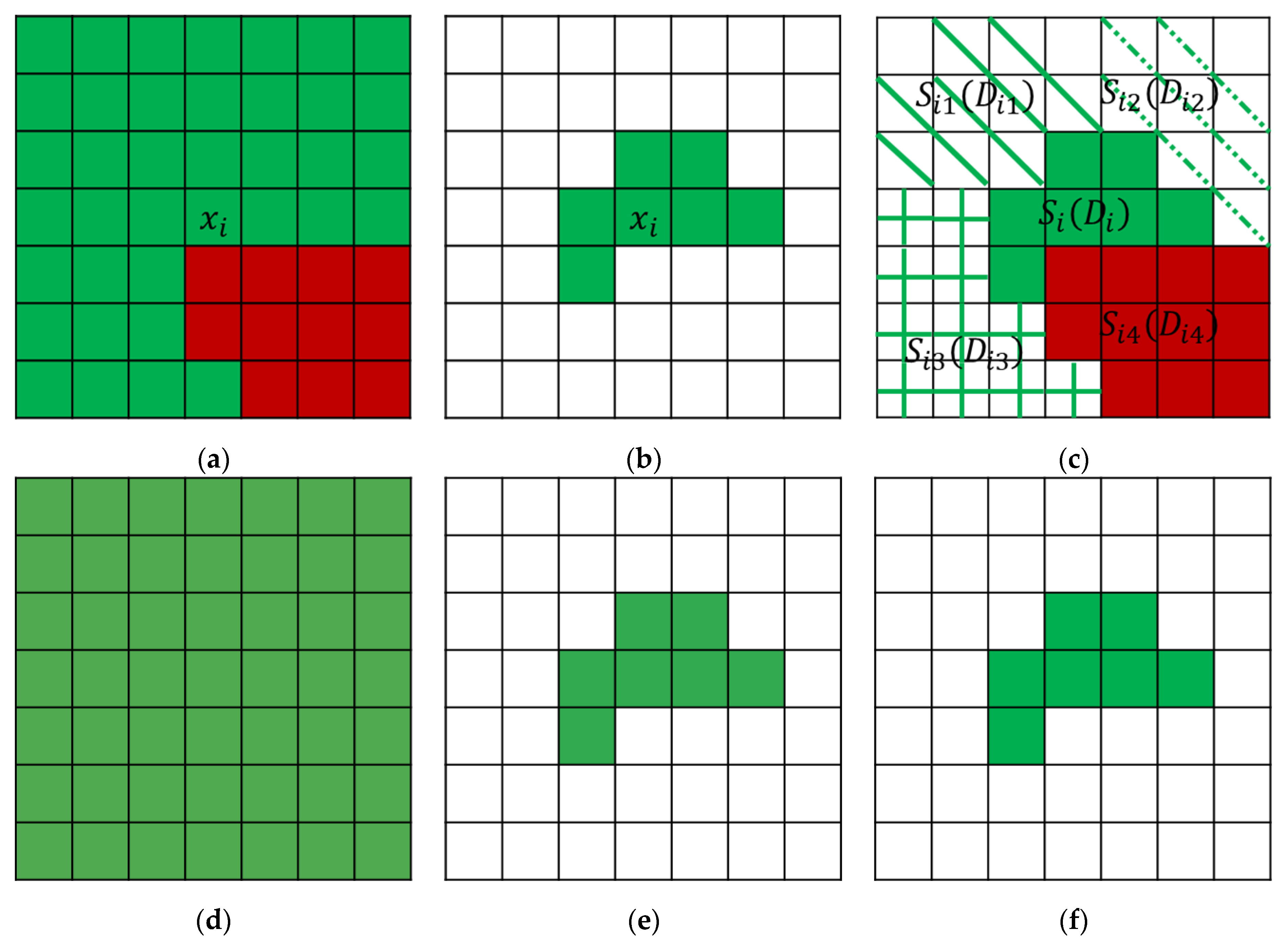
We proposed the WASCK method to classify the HSI by utilizing the spectral-spatial features. The spatial neighborhood used in CK is constructed in a square region centered on each target pixel, which makes the objects be affected by backgrounds. In order to reduce this effect, the SCK method uses the information of superpixels to find the homogeneous region. Furthermore, we use adjacent superpixels information and its location information of each superpixel to construct a weighted ASs. The weighted ASs strategy can reduce the impact of undesired superpixels by assigning different weights to adjacent superpixels. Figure 1 shows a simple example of different spatial region selection strategies. It can be seen that there are two different ground object targets, denoted as green and red respectively. Figure 1a–c show the strategies of the square neighborhood, superpixel neighborhood and weighted ASs neighborhood, respectively. Figure 1d–f show the corresponding features extracted under three strategies. Since the size of square neighborhood is artificially chosen and fixed, for a target pixel , if the size is too large, it will contain irrelevant pixels (i.e., red pixel). On the contrary, if the size is too small, more effective spatial information cannot be considered. It is difficult to find a suitable size for all target pixels, so the spatial features cannot be fully extracted to the classification (see Figure 1d). Figure 1b is the superpixel-based strategy. The size and shape of each superpixel can be adapted to vary based on different spatial structures. However, this strategy may cause the problem that each superpixel is too small to obtain effective spatial information on account of over-segmentation (see Figure 1e). Figure 1c is the weighted ASs-based strategy, where are superpixels adjacent to the target superpixel and are the corresponding centroids. By assigning smaller weights to dissimilar superpixels (i.e., ), this strategy can maintain ASs-based homogeneous regions to a large extent, and effectively reduce the adverse effects of dissimilar superpixels. The color of feature also demonstrates that the weighted ASs neighborhood will produce the most accurate result (see Figure 1f). Therefore, the weighted ASs strategy can effectively exploit spatial-spectral features of ASs.
The WASCK method integrates the weighted ASs strategy and CK together. Let be the HSI, where is the depth of HSI and is the number of pixels. Firstly, given a superpixel number , the HSI can be segmented into superpixels by ERS on the first PC image. For each superpixel , its adjacent superpixels can be denoted as , where is the number of adjacent superpixels. At the same time, we can get the corresponding centroids to each adjacent superpixel. Since the feature of each superpixel can be represented by its mean pixel , the weight of each superpixel can also be calculated by (). In order to exploit spatial features and location information of adjacent superpixels, the spatial information of can be denoted as:
where and represent the correlation of location information and spatial information between the current superpixel and its adjacent superpixels, respectively. and are the broadband parameter of the function, which controls the radial action range. Then, the WASCK we constructed can be expressed as follows:
After the kernel function is obtained, the decision formula is obtained by substituting Equation (11) into Equation (3).
3.2. Multiscale Weighted Adjacent Superpixel-Based Composite Kernel (MWASCK)
The WASCK method only uses the single-scale weighted ASs to extract the spatial features. Here, the fusion of superpixel spatial information under different segmentation scales is considered to improve classification performance. Considering that it is possible to avoid seeking for the optimal superpixel scale and fuse the spatial multiscale features, the MWASCK method is utilized in the framework of WASCK as follows:
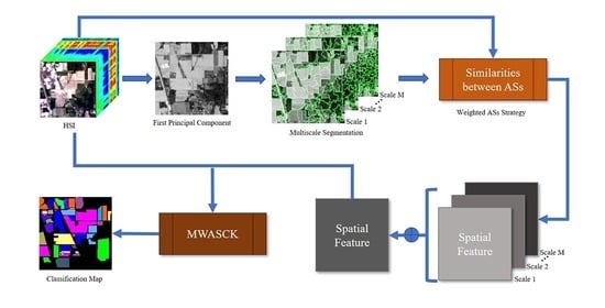
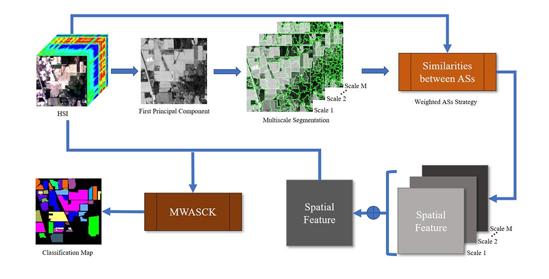
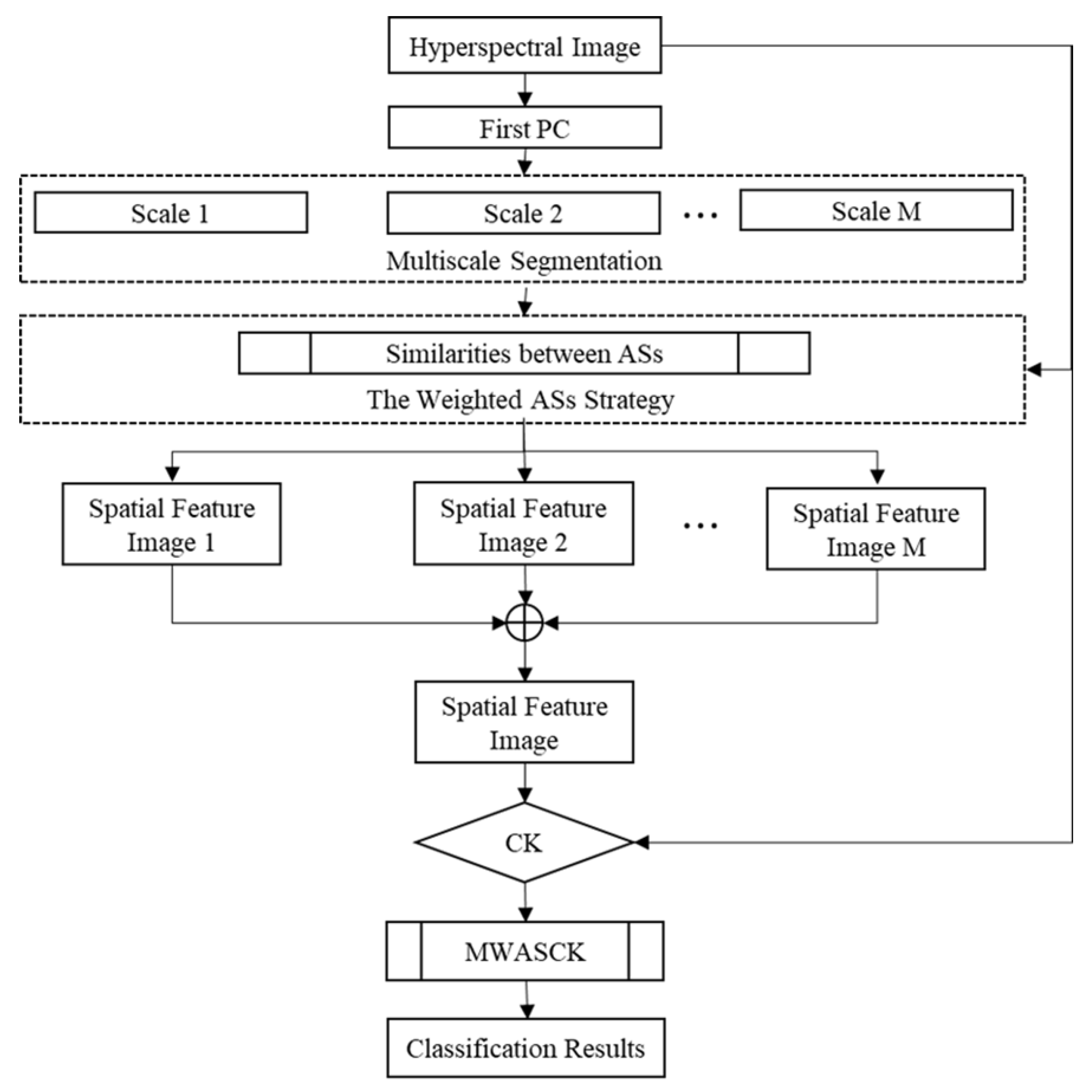
where can be selected empirically and represents the number of total scales. can be acquired by the spatial kernel of Equation (11) directly and represents spatial kernel on scale . As in the above case, we can obtain the decision formula by substituting Equation (12) into Equation (3). Figure 2 shows the flowchart of using weighted ASs features to classify HSI via MWASCK.
4. Experimental Results
4.1. Datasets
Indian Pines: This is a image taken from a test site for Indian Pine in Northwest Indiana by AVIRIS sensor. Each pixel in the image contains 220 wavelengths, covering wavelengths from 0.4 to 2.5 m. By removing the 20 wavelengths that are absorbed by water vapor we end up with 200 wavelengths. Table 1 details the 16 available reference categories. The training samples required for the experiment are randomly selected from 3% of each category and the rest for testing.
University of Pavia: This is a image taken from the University of Pavia by ROSIS sensor. Each pixel in the image contains 115 wavelengths, covering a wavelength from 0.43 to 0.86 m. By removing 12 wavelengths affected by the noise we end up with 103 wavelengths. Table 1 details the 9 available reference categories. The training samples required for the experiment are randomly selected from 30 of each category and the rest for testing.
4.2. Experimental Results
In the experiments, several kernel-based classification methods are used to compare with our method: support vector machine with RBF kernel (SVM-RBF) [6] method, the classic support vector machine with composite kernel (SVMCK) [31] method, the superpixel-based multiple kernels (SCMK) [45] method, the relaxed multiple kernel based on region (RMK) [46] method and the multiscale spatial-spectral kernel based on adjacent superpixel (ASMGSSK) [47]. The overall accuracy (OA), average accuracy (AA) and Kappa coefficient are used as evaluation criterion of algorithm performance. Moreover, the average results of ten randomized tests are used as the final experimental data. The optimal parameters of the proposed WASCK and MASCK approaches are set as follows. For proposed methods, the value chosen for spectral kernel weight is 0.1, the value chosen for is , the and in Equation (5) are set to , the in Equation (6) is set to in Indian Pines dataset and is set to in University of Pavia dataset. To simplify the statement, we use to represent the number of superpixels. The optimal for the WASCK is set to 1400 in Indian Pines dataset and is set to 1100 in University of Pavia dataset. The multiscale for the MWASCK is set to in Indian Pines dataset and is set to in University of Pavia dataset. The comparison methods choose their optimal parameter settings. In addition, after fivefold cross-validation, SVM training parameters are selected. The multiple methods based on SVM in this paper are calculated by using LIBSVM [51] toolbox.
Figure 3 and Figure 4 show classification maps of multiple approaches for two datasets. Obviously, the map of SVM-RBF method shows many noisy estimations, which only considers the spectral information. SVMCK method uses the spatial features of HSI to acquire a smoother classification map. However, the detail and edge regions still have a lot of misclassified pixels. The SCMK and RMK methods achieve better classification maps by considering the multiple kernels and the spatial information of ASs. The ASMGSSK method further achieves satisfactory classification maps by integrating the ASs strategy and multiscale feature fusion together. Moreover, the WASCK method also provides a smoother classification map and maintains the details. The MWASCK approach achieves the best classification map than the other compared classifiers by considering the weighted ASs strategy and multiscale structures of HSI.
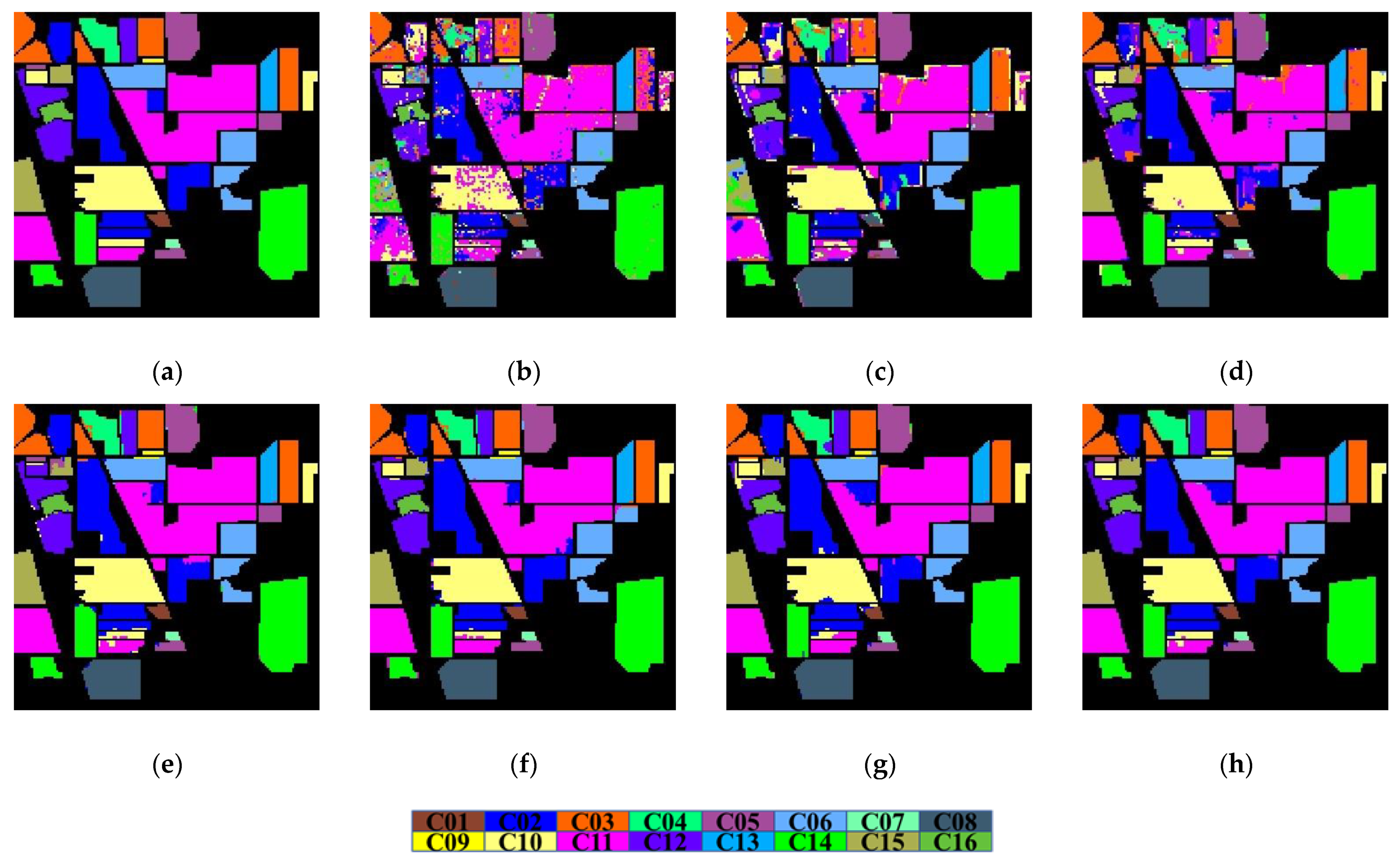
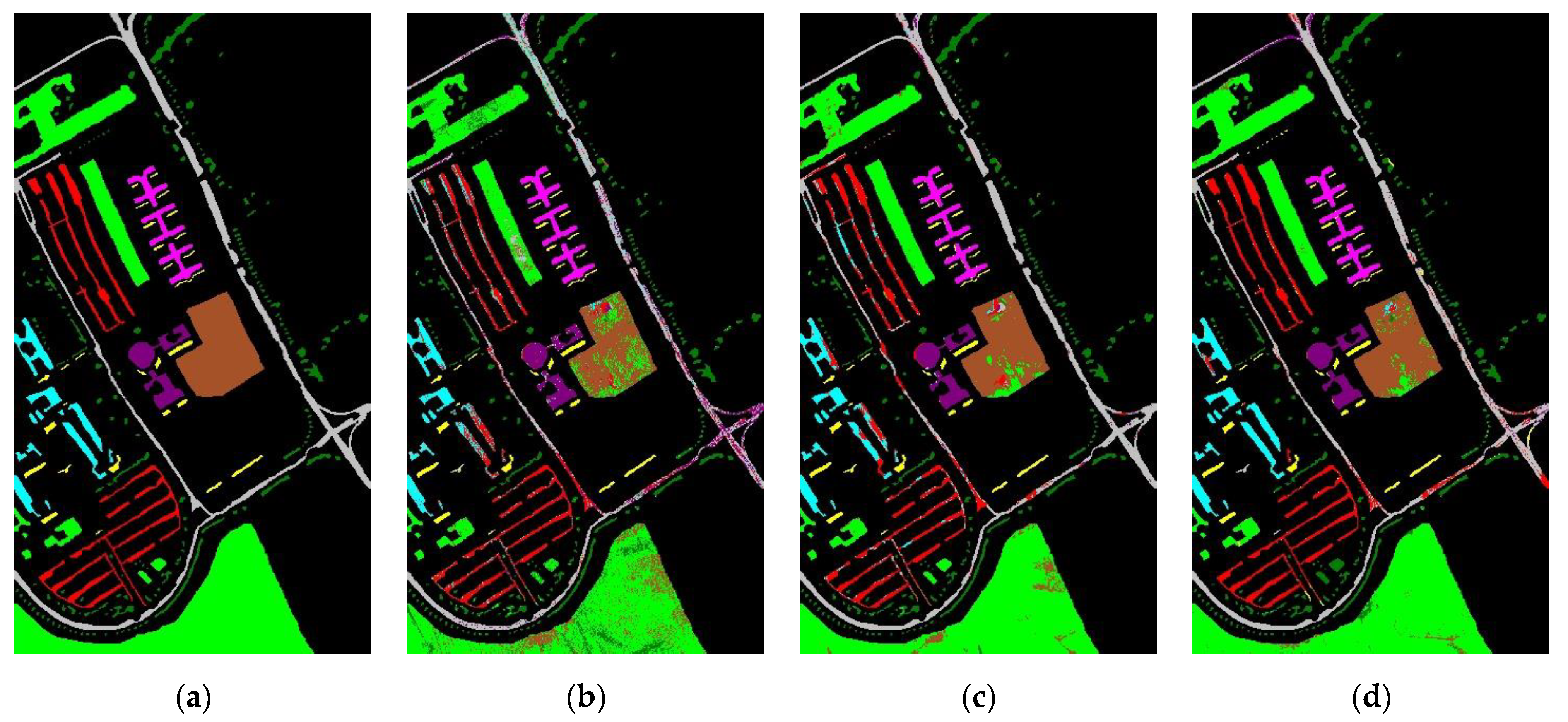
Table 2 and Table 3 present the experimental data of multiple approaches for two datasets. Obviously, SVM-RBF method achieves very poor accuracy, which only considers the spectral features. The SVMCK method improves the OA value by adding spatial features within a square region. SCMK and RMK methods achieve higher accuracy by considering the multiple kernels and spatial information of ASs, respectively. By taking into consideration the spatial features of the ASs and multiscale structures of HSI, The ASMGSSK method also achieves satisfactory classification accuracy. In addition, the WASCK approach has obtained excellent classification accuracy by considering the weighted ASs strategy. Moreover, the MWASCK method achieves the best accuracy than the other compared classifiers by considering the weighted ASs strategy and multiscale structures of HSI.
Deep learning approaches have been used to classify HSIs in recent years. This paper also compares several excellent CNN-based deep learning methods: the deep CNN [52] method, the CNN based on contextual deep (CD-CNN) [53] method and the CNN based on diverse region (DR-CNN) [54] method. Table 4 shows the classification accuracies under the selection of different number of training samples in each category. For Indian Pines dataset, we only chose to use the first nine larger categories. Obviously, in the case of a small number of training samples, the MWASCK shows a better classification result compared with the deep learning methods. Since CNN needs more training samples to reach its maximum capacity. Therefore, the advantage of our method is that it still has excellent classification performance when the training samples are limited. In addition, we further compared the MWASCK with another a fully dense multiscale fusion network (FDMFN) [55] method under the same training samples on the Indian Pines and Kennedy Space Center (KSC) datasets. The details of the KSC datasets can be found in [55]. The classification results are shown in Table 5. Obviously, our method also shows an outstanding classification performance.
4.3. Discussion
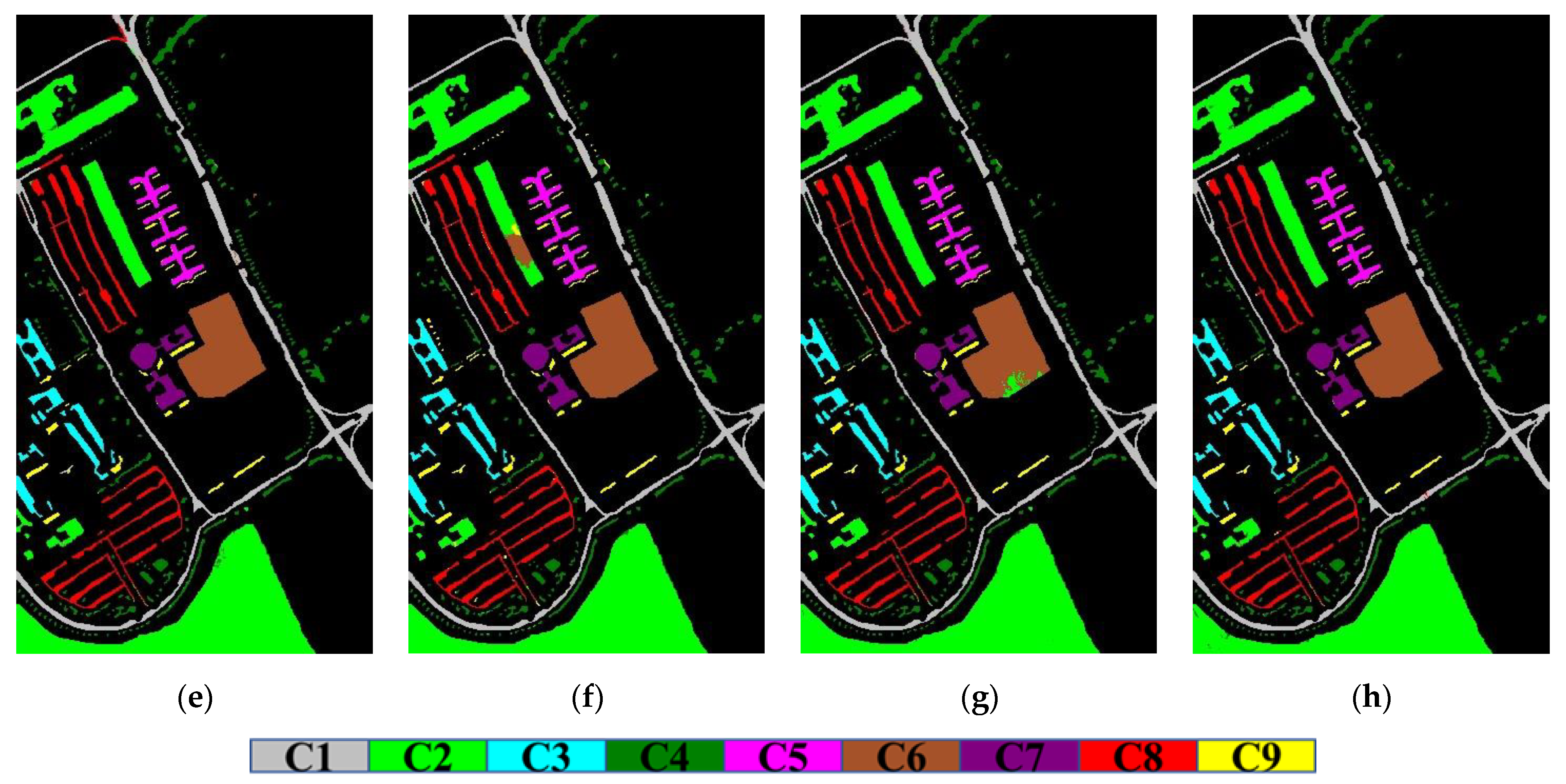
Figure 5 illustrates the line graph of the OA values of WASCK method under different number of superpixels (). The weighted ASs-based strategy requires smaller size of superpixels to form larger homogeneous regions. Hence, when is large, the WASCK has better classification performance. However, it will result in over-segmentation and cannot extract spatial information effectively when is too large, and then the classification performance will decline. As it can be observed, the optimal for two datasets is 1400 and 1100, respectively. It can also be found that when the optimal is exceeded, classification performance of the WASCK will degrade.
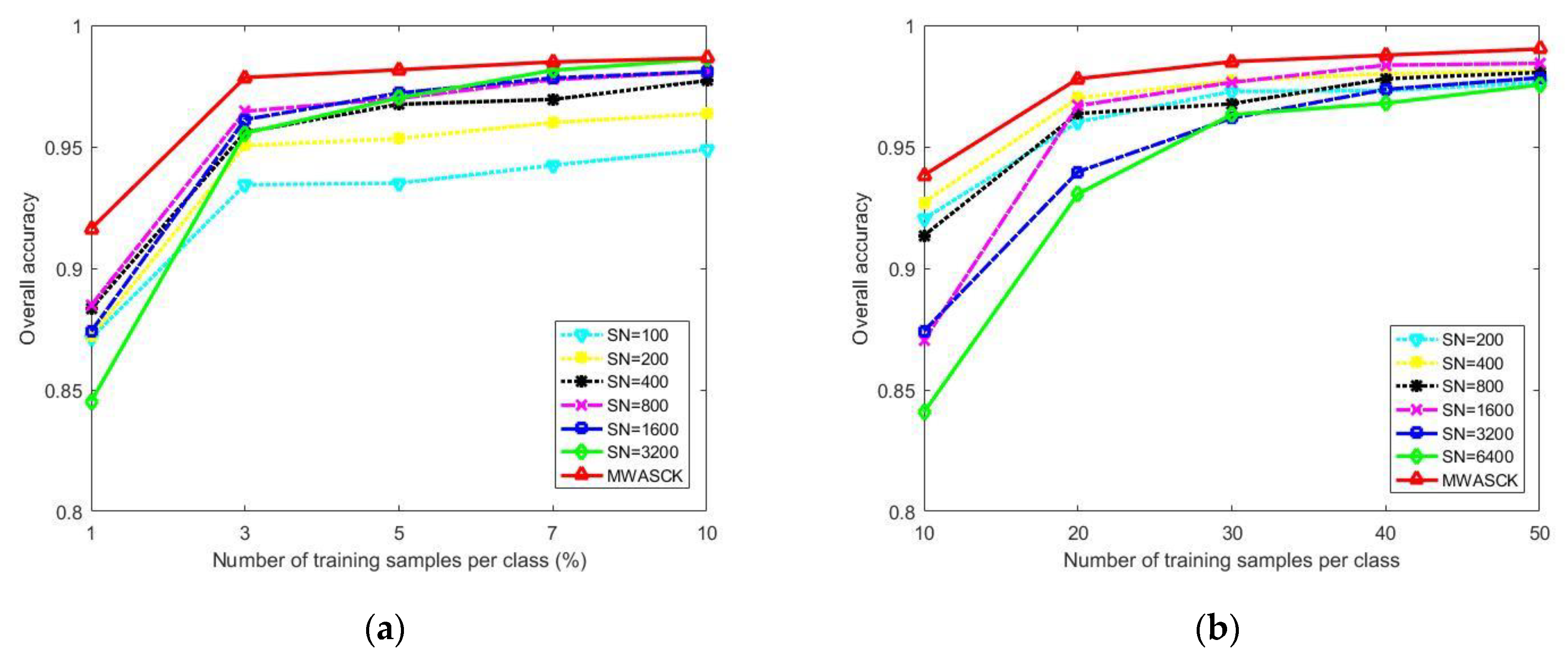
Figure 6 illustrates the OA values of single-scale and multi-scale MWASCK under different training samples. SN marked in the figure represents the number of superpixels. Obviously, with a limited training sample, single-scale MWASCK with fewer superpixels can obtain higher OA, while single-scale MWASCK with more superpixels can obtain higher OA with sufficient training samples. Therefore, it has been confirmed that spatial information cannot be effectively utilized by small scale superpixels with limited labeled samples. In addition, when a large number of superpixels are selected to achieve better experimental data, the spatial information of weighted ASs cannot be exploited effectively, resulting in poor classification performance (see SN = 3200 and SN = 6400 in Figure 6b). Meanwhile, when enough training samples are selected, the limitation of the segmentation algorithm will lead to the failure to improve the OA value. The proposed MWASCK method not only improves the OA values, but also avoids selecting the optimal and sufficient number of samples.
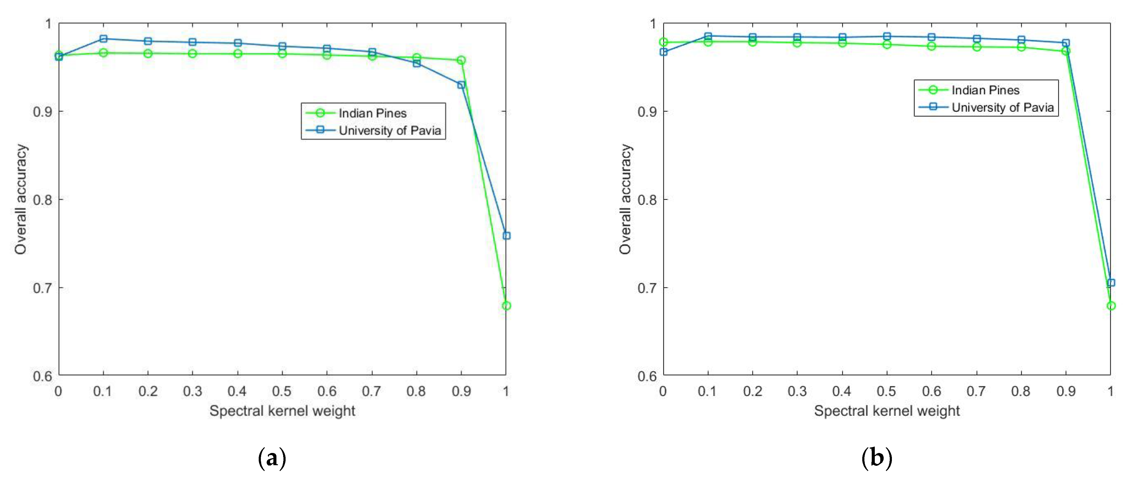
Figure 7 illustrates the effect of the spectral kernel weight associated with WASCK and MWASCK. The interval between 0 and 1 as the value of the spectral kernel weight. Obviously, the WASCK and MWASCK show poor classification performance on two datasets when we assign a value of 0 or 1 to the spectral kernel weight (i.e., only using spatial features of weighted ASs or spectral features). On the contrary, the proposed methods show good classification performance when the spatial information is utilized (i.e., the spectral kernel varies from 0.1 to 0.9). This suggests that we should combine spectral features with spatial features of the weighted ASs to classify HSI. It is worth noting that when the interval between 0.1 and 0.9 as the value of the spectral kernel weight, the performance of the proposed methods on two datasets generally degrades. This tells us that we should assign a relatively large weight to the spatial kernel.
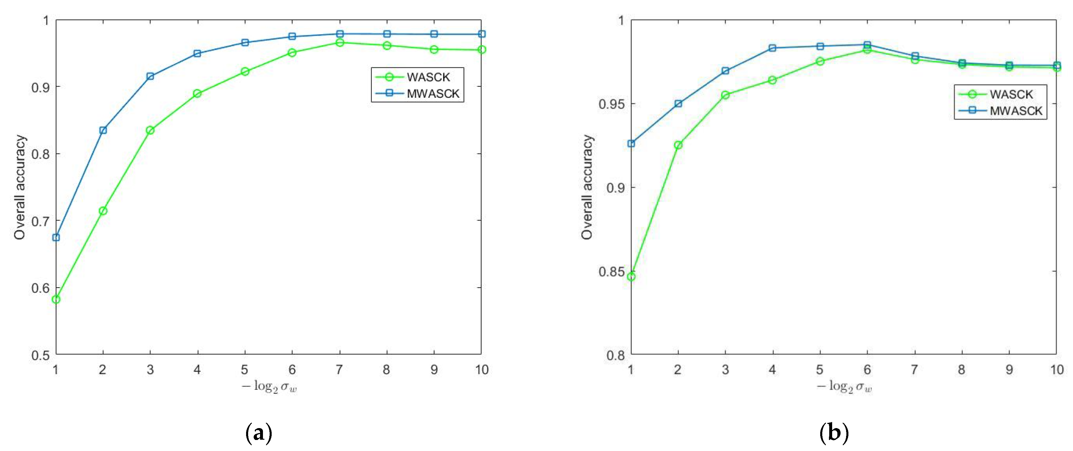
Figure 8 illustrates the effect of the kernel width on two datasets. We can observe that the MWASCK has a more robust kernel width value than WASCK. Meanwhile, the proposed WASCK and MWASCK can show better classification performance when goes from to on Indian Pines dataset and goes from to on University of Pavia dataset.
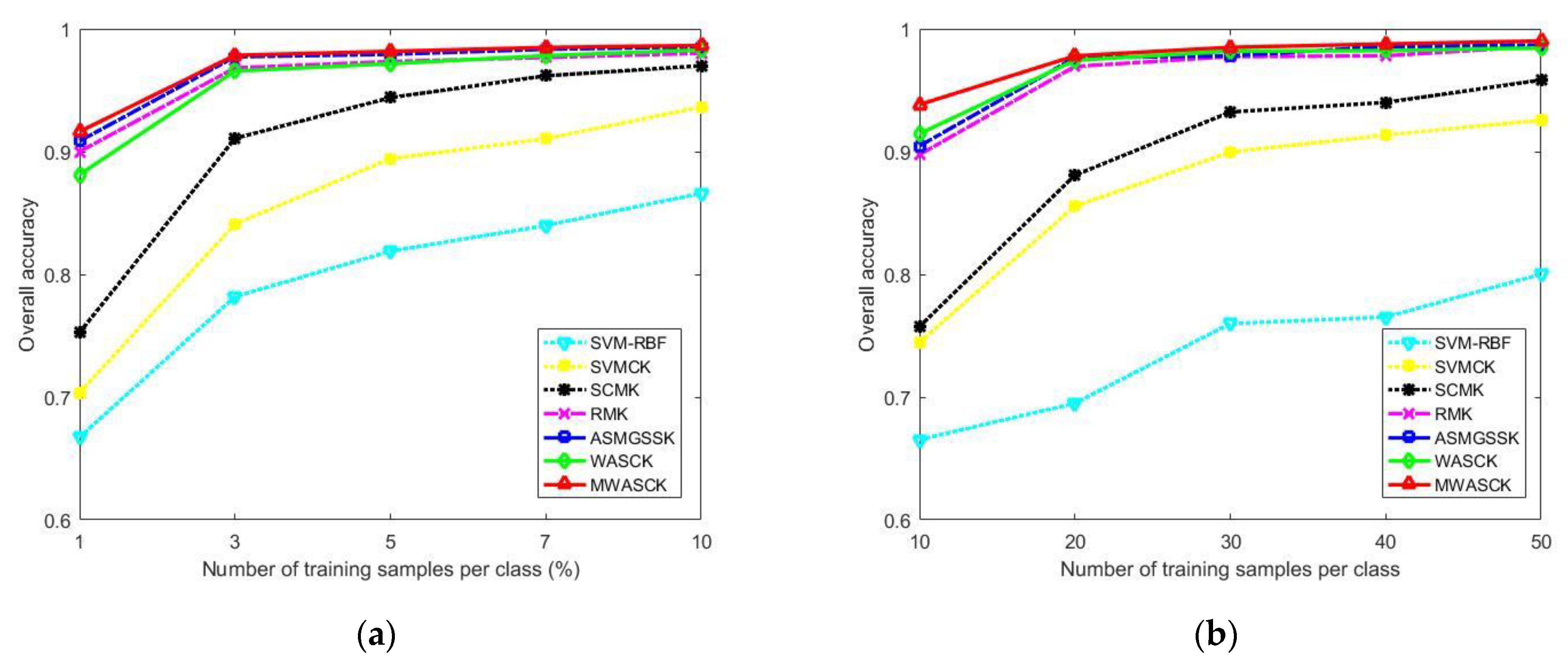
Figure 9 shows the line chart of OA values of several methods for two datasets under different training sample numbers. As can be observed, with the increase of training sample numbers, classification accuracy is getting higher and higher. At the same time, the WASCK and MWASCK methods provide superior performance compared with other classification approaches. It is worth noting that classification accuracies of the MWASCK are higher than other compared methods on different training samples.
Table 6 presents the time costs of the WASCK and MWASCK on the Indian Pines dataset and University of Pavia dataset. All of our experiments are run on a laptop computer with an Intel Core i5-8265U CPU 1.60 GHz and 8GB of RAM. Obviously, the superpixel segmentation and kernels computation processes take up most of the computation time. In addition, since the segmentation algorithm in [43] is efficient, the superpixel segmentation stage does not consume much time. For the MWASCK on the University of Pavia dataset, since the maximum number of superpixel segmentation reaches 6400, the calculation cost of segmentation and kernels computation is greatly increased. It is worth noting that once the segmentation of superpixels has been completed, the pixels within each superpixel share the same spatial information, and additional costs of this process will not increase with the increase of the number of samples.
5. Conclusions
In this paper, WASCK and MWASCK methods are proposed to classify the HSI. The WASCK fully utilizes spatial and location information of the weighted ASs. In addition, the multiscale method is adopted in the framework of WASCK (i.e., MWASCK) to effectively exploit multiscale superpixel spatial and location information of the HSI. Experiment results have indicated that the WASCK and MWASCK achieve the desired excellent classification performance.
In the experiments, the optimal spectral kernel weight was not selected for each test pixel. The spectral kernel weight was only selected as a fixed value empirically and used jointly by all the test pixels. Therefore, the optimal spectral kernel weight can be obtained adaptively through the local distribution of target pixels. In addition, an excellent superpixel segmentation technique will also show better classification performance.
In the future, deep features [56,57,58,59] will be considered to be exploited and integrated into the composite kernel framework for obtaining more accurate results. Moreover, how to adaptively decide the weight of each base kernel is also an open problem, optimal algorithm such as particle swarm optimization [60,61] will be considered and studied.
Author Contributions
Conceptualization, Y.C.; Methodology, Y.C.; Software, Y.Z.; validation, Y.Z. and Y.C.; Formal analysis, Y.C.; Investigation, Y.Z. and Y.C.; Resources, Y.C.; data curation, Y.Z.; writing—original draft preparation, Y.Z. and Y.C.; writing—review and editing, Y.C.; visualization, Y.Z.; supervision, Y.C.; project administration, Y.C.; funding acquisition, Y.C. All authors have read and agreed to the published version of the manuscript.
Funding
This research was funded by the National Nature Science Foundation of China, grant number 61672291 and the Six talent peaks project in Jiangsu Province, grant number SWYY-034.
Institutional Review Board Statement
Not applicable.
Informed Consent Statement
Not applicable.
Data Availability Statement
Data available in a publicly accessible repository.
Acknowledgments
We thank Tianming Zhan for providing technical assistance.
Conflicts of Interest
The authors declare no conflict of interest.
References
- Bioucas-Dias, J.M.; Plaza, A.; Camps-Valls, G.; Scheunders, P.; Nasrabadi, N. Hyperspectral Remote Sensing Data Analysis and Future Challenges. IEEE Geosci. Remote Sens. Mag. 2013, 1, 6–36. [Google Scholar] [CrossRef] [Green Version]
- Tu, B.; Zhou, C.; He, D.; Huang, S.; Plaza, A. Hyperspectral Classification with Noisy Label Detection via Superpixel-to-Pixel Weighting Distance. IEEE Trans. Geosci. Remote Sens. 2020, 58, 4116–4131. [Google Scholar] [CrossRef]
- Jin, Q.; Ma, Y.; Mei, X.; Dai, X.; Huang, J. Gaussian Mixture Model for Hyperspectral Unmixing with Low-Rank Representation. In Proceedings of the IGARSS 2019 IEEE International Geoscience and Remote Sensing Symposium, Yokohama, Japan, 28 July–2 August 2019; pp. 294–297. [Google Scholar]
- Zhang, L.; Zhang, L.; Tao, D.; Huang, X.; Du, B. Hyperspectral Remote Sensing Image Subpixel Target Detection Based on Supervised Metric Learning. IEEE Trans. Geosci. Remote Sens. 2014, 52, 4955–4965. [Google Scholar] [CrossRef]
- Hou, Y.; Zhu, W.; Wang, E. Hyperspectral Mineral Target Detection Based on Density Peak. Intell. Autom. Soft Comput. 2019, 25, 805–814. [Google Scholar] [CrossRef]
- Melgani, F.; Bruzzone, L. Classification of Hyperspectral Remote Sensing Images with Support Vector Machines. IEEE Trans. Geosci. Remote Sens. 2004, 42, 1778–1790. [Google Scholar] [CrossRef] [Green Version]
- Jia, X.; Richards, J.A. Segmented principal components transformation for efficient hyperspectral remote-sensing image display and classification. IEEE Trans. Geosci. Remote Sens. 1999, 37, 538–542. [Google Scholar]
- Liu, J.; Xiao, Z.; Chen, Y.; Yang, J. Spatial-Spectral Graph Regularized Kernel Sparse Representation for Hyperspectral Image Classification. Int. J. Geo. Inf. 2017, 6, 258. [Google Scholar] [CrossRef]
- Ye, Q.; Yang, J.; Liu, F.; Zhao, C.; Ye, N.; Yin, T. L1-Norm Distance Linear Discriminant Analysis Based on an Effective Iterative Algorithm. IEEE Trans. Circuits Syst. Video Technol. 2018, 28, 114–129. [Google Scholar] [CrossRef]
- Ye, Q.; Zhao, H.; Li, Z.; Yang, X.; Gao, S.; Yin, T.; Ye, N. L1-norm Distance Minimization Based Fast Robust Twin Support Vector k-plane Clustering. IEEE Trans. Neural Netw. Learn. Syst. 2018, 29, 4494–4503. [Google Scholar] [CrossRef] [PubMed]
- Ma, Y.; Li, C.; Li, H.; Mei, X.; Ma, J. Hyperspectral Image Classification with Discriminative Kernel Collaborative Representation and Tikhonov Regularization. IEEE Geosci. Remote Sens. Lett. 2018, 15, 587–591. [Google Scholar] [CrossRef]
- Zhao, G.; Tu, B.; Fei, H.; Li, N.; Yang, X. Spatial-Spectral Classification of Hyperspectral Image via Group Tensor Decomposition. Neurocomputing 2018, 316, 68–77. [Google Scholar] [CrossRef]
- Quesada-Barriuso, P.; Arguello, F.; Heras, D.B. Spectral–Spatial Classification of Hyperspectral Images Using Wavelets and Extended Morphological Profiles. IEEE J. Sel. Top. Appl. Earth Observ. Remote Sens. 2014, 7, 1177–1185. [Google Scholar] [CrossRef]
- Li, W.; Du, Q. Gabor-Filtering-Based Nearest Regularized Subspace for Hyperspectral Image Classification. IEEE J. Sel. Top. Appl. Earth Observ. Remote Sens. 2014, 7, 1012–1022. [Google Scholar] [CrossRef]
- Shen, L.; Jia, S. Three-Dimensional Gabor Wavelets for Pixel-Based Hyperspectral Imagery Classification. IEEE Trans. Geosci. Remote Sens. 2011, 49, 5039–5046. [Google Scholar] [CrossRef]
- Benediktsson, J.A.; Palmason, J.A.; Sveinsson, J.R. Classification of Hyperspectral Data from Urban Areas Based on Extended Morphological Profiles. IEEE Trans. Geosci. Remote Sens. 2005, 43, 480–491. [Google Scholar] [CrossRef]
- Tarabalka, Y.; Fauvel, M.; Chanussot, J.; Benediktsson, J.M. SVM and MRF-Based Method for Accurate Classification of Hyperspectral Images. IEEE Trans. Geosci. Remote Sens. 2010, 7, 736–740. [Google Scholar] [CrossRef] [Green Version]
- Li, J.; Bioucas-Dias, J.M.; Plaza, A. Spectral–Spatial Hyperspectral Image Segmentation Using Subspace Multinomial Logistic Regression and Markov Random Fields. IEEE Trans. Geosci. Remote Sens. 2012, 50, 809–823. [Google Scholar] [CrossRef]
- Sun, L.; Wu, Z.; Liu, J.; Xiao, L.; Wei, Z. Supervised Spectral–Spatial Hyperspectral Image Classification with Weighted Markov Random Fields. IEEE Trans. Geosci. Remote Sens. 2015, 53, 1490–1503. [Google Scholar] [CrossRef]
- Chen, Y.; Nasrabadi, N.M.; Tran, T.D. Hyperspectral Image Classification Using Dictionary-Based Sparse Representation. IEEE Trans. Geosci. Remote Sens. 2011, 49, 3973–3985. [Google Scholar] [CrossRef]
- Li, W.; Du, Q. Joint Within-Class Collaborative Representation for Hyperspectral Image Classification. IEEE J. Sel. Top. Appl. Earth Observ. Remote Sens. 2014, 7, 2200–2208. [Google Scholar] [CrossRef]
- Pan, C.; Li, J.; Wang, Y.; Gao, X. Collaborative learning for hyperspectral image classification. Neurocomputing 2017, 275, 2512–2524. [Google Scholar] [CrossRef]
- Fu, L.; Li, Z.; Ye, Q.; Yin, H.; Liu, Q.; Chen, X.; Fan, X.; Yang, W.; Yang, G. Learning Robust Discriminant Subspace Based on Joint L2,p- and L2,s-Norm Distance Metrics. IEEE Trans. Neural Netw. Learn. Syst. 2020. [Google Scholar] [CrossRef]
- Ye, Q.; Li, Z.; Fu, L.; Yang, W.; Yang, G. Nonpeaked Discriminant Analysis for Data Representation. IEEE Trans. Neural Netw. Learn. Syst. 2019, 30, 3818–3832. [Google Scholar] [CrossRef] [PubMed]
- He, Z.; Wang, Y.; Hu, J. Joint Sparse and Low-Rank Multitask Learning with Laplacian-Like Regularization for Hyperspectral Classification. Remote Sens. 2018, 10, 322. [Google Scholar] [CrossRef] [Green Version]
- Du, L.; Wu, Z.; Xu, Y.; Liu, W.; Wei, Z. Kernel Low-Rank Representation for Hyperspectral Image Classification. In Proceedings of the 2016 IEEE International Geoscience and Remote Sensing Symposium, Beijing, China, 10–15 July 2016; pp. 477–480. [Google Scholar]
- Yuebin, W.; Jie, M.; Liqiang, Z.; Bing, Z.; Anjian, L.; Yibo, Z. Self-Supervised Low-rank Representation (SSLRR) for Hyperspectral Image Classification. IEEE Trans. Geosci. Remote Sens. 2018, 56, 5658–5672. [Google Scholar]
- Sun, L.; Ma, C.; Chen, Y.; Zheng, Y.; Jeon, B. Low rank component induced spatial-spectral kernel method for hyperspectral image classification. IEEE Trans. Cir. Sys. Video Tech. 2020, 30, 3829–3842. [Google Scholar] [CrossRef]
- Sun, L.; He, C.; Zheng, Y.; Tang, S. SLRL4D: Joint restoration of subspace low-rank learning and non-local 4-D transform filtering for hyperspectral image. Remote Sens. 2020, 12, 2979. [Google Scholar] [CrossRef]
- Sun, L.; Wu, F.; He, C.; Zhan, T.; Liu, W.; Zhang, D. Weighted Collaborative Sparse and L1/2 Low-Rank Regularizations With Superpixel Segmentation for Hyperspectral Unmixing. IEEE Geosci. Remote Sens. Lett. 2020. [CrossRef]
- Camps-Valls, G.; Gomez-Chova, L.; Munoz-Mari, J.; Vila-Frances, J.; Calpe-Maravilla, J. Composite Kernels for Hyperspectral Image Classification. IEEE Geosci. Remote Sens. Lett. 2006, 3, 93–97. [Google Scholar] [CrossRef]
- Zhou, Y.; Peng, J.; Chen, C.L.P. Extreme Learning Machine with Composite Kernels for Hyperspectral Image Classification. IEEE J. Sel. Top. Appl. Earth Observ. Remote Sens. 2015, 8, 2351–2360. [Google Scholar] [CrossRef]
- Li, H.; Ye, Z.; Xiao, G. Hyperspectral Image Classification Using Spectral–Spatial Composite Kernels Discriminant Analysis. IEEE J. Sel. Top. Appl. Earth Observ. Remote Sens. 2015, 8, 2341–2350. [Google Scholar] [CrossRef]
- Zhang, Y.; Prasad, S. Locality Preserving Composite Kernel Feature Extraction for Multi-Source Geospatial Image Analysis. IEEE J. Sel. Top. Appl. Earth Observ. Remote Sens. 2015, 8, 1385–1392. [Google Scholar] [CrossRef]
- Gomez-Chova, L.; Camps-Valls, G.; Bruzzone, L.; Calpe-Maravilla, J. Mean Map Kernel Methods for Semisupervised Cloud Classification. IEEE Trans. Geosci. Remote Sens. 2010, 48, 207–220. [Google Scholar] [CrossRef]
- Camps-Valls, G.; Shervashidze, N.; Borgwardt, K.M. Spatio-Spectral Remote Sensing Image Classification with Graph Kernels. IEEE Geosci. Remote Sens. Lett. 2010, 7, 741–745. [Google Scholar] [CrossRef]
- Wang, J.; Jiao, L.; Liu, H.; Yang, S.; Liu, F. Hyperspectral Image Classification by Spatial–Spectral Derivative-Aided Kernel Joint Sparse Representation. IEEE J. Sel. Top. Appl. Earth Observ. Remote Sens. 2015, 8, 2485–2500. [Google Scholar] [CrossRef]
- Zhang, H.; Li, J.; Huang, Y.; Zhang, L. A Nonlocal Weighted Joint Sparse Representation Classification Method for Hyperspectral Imagery. IEEE J. Sel. Top. Appl. Earth Observ. Remote Sens. 2014, 7, 2056–2065. [Google Scholar] [CrossRef]
- Li, J.; Zhang, H.; Huang, Y.; Zhang, L. Hyperspectral Image Classification by Nonlocal Joint Collaborative Representation with a Locally Adaptive Dictionary. IEEE Trans. Geosci. Remote Sens. 2014, 52, 3707–3719. [Google Scholar] [CrossRef]
- Wang, J.; Jiao, L.; Wang, S.; Hou, B.; Liu, F. Adaptive Nonlocal Spatial–Spectral Kernel for Hyperspectral Imagery Classification. IEEE J. Sel. Top. Appl. Earth Observ. Remote Sens. 2016, 9, 4086–4101. [Google Scholar] [CrossRef]
- Mori, G.; Ren, X.; Efros, A.A.; Malik, J. Recovering human body configurations: Combining segmentation and recognition. In Proceedings of the 2004 IEEE Computer Society Conference on Computer Vision and Pattern Recognition, Washington, DC, USA, 27 June–2 July 2004; pp. 326–333. [Google Scholar]
- Caliskan, A.; Bati, E.; Koza, A.; Alatan, A.A. Superpixel based hyperspectral target detection. In Proceedings of the 2016 IEEE International Geoscience and Remote Sensing Symposium (IGARSS), Beijing, China, 10–15 July 2016; pp. 7010–7013. [Google Scholar]
- Liu, M.Y.; Tuzel, O.; Ramalingam, S.; Chellappa, R. Entropy rate superpixel segmentation. In Proceedings of the 2011 IEEE Computer Society Conference on Computer Vision and Pattern Recognition, Colorado Springs, CO, USA, 20–25 June 2011; pp. 2097–2104. [Google Scholar]
- Duan, W.; Li, S.; Fang, L. Superpixel-based composite kernel for hyperspectral image classification. In Proceedings of the 2015 IEEE International Geoscience and Remote Sensing Symposium (IGARSS), Milan, Italy, 26–31 July 2015; pp. 1698–1701. [Google Scholar]
- Fang, L.; Li, S.; Duan, W.; Ren, J.; Benediktsson, J.A. Classification of Hyperspectral Images by Exploiting Spectral–Spatial Information of Superpixel via Multiple Kernels. IEEE Trans. Geosci. Remote Sens. 2015, 53, 6663–6674. [Google Scholar] [CrossRef] [Green Version]
- Liu, J.; Wu, Z.; Xiao, Z.; Yang, J. Region-based relaxed multiple kernel collaborative representation for hyperspectral image classification. IEEE Access 2017, 5, 20921–20933. [Google Scholar] [CrossRef]
- Sun, L.; Ma, C.; Chen, Y.; Shim, H.J.; Wu, Z.; Jeon, B. Adjacent superpixel-based multiscale spatial-spectral kernel for hyperspectral classification. IEEE J. Sel. Top. Appl. Earth Observ. Remote Sens. 2019, 12, 1905–1919. [Google Scholar] [CrossRef]
- Aizerman, M.A.; Braverman, È.M.; Rozonoèr, L.I. Theoretical foundation of potential functions method in pattern recognition. Avtomat. Telemekh. 1964, 25, 917–936. [Google Scholar]
- Hervé, A.; Williams, L.J. Principal component analysis. Wiley Interd. Rev. Comput. Stats. 2010, 2, 433–459. [Google Scholar]
- Nemhauser, G.L.; Wolsey, L.A.; Fisher, M.L. An analysis of approximations for maximizing submodular set functions—I. Math. Prog. 1978, 14, 265–294. [Google Scholar] [CrossRef]
- Chang, C.-C.; Lin, C.-J. Libsvm: A library for support vector machines. ACM Trans. Intelligent Sys. Tech. 2011, 2, 27. [Google Scholar] [CrossRef]
- Hu, W.; Huang, Y.; Wei, L.; Zhang, F.; Li, H. Deep convolutional neural networks for hyperspectral image classification. J. Sens. 2015, 2015, 1–12. [Google Scholar] [CrossRef] [Green Version]
- Lee, H.; Kwon, H. Going deeper with contextual cnn for hyperspectral image classification. IEEE Trans. Image Process. 2017, 26, 4843–4855. [Google Scholar] [CrossRef] [Green Version]
- Zhang, M.; Li, W.; Du, Q. Diverse Region-Based CNN for Hyperspectral Image Classification. IEEE Trans. Image Process. 2018, 27, 2623–2634. [Google Scholar] [CrossRef]
- Meng, Z.; Li, L.; Jiao, L.; Feng, Z.; Liang, M. Fully dense multiscale fusion network for hyperspectral image classification. Remote Sens. 2019, 11, 2718. [Google Scholar] [CrossRef] [Green Version]
- Xu, F.; Zhang, X.; Xin, Z.; Yang, A. Investigation on the Chinese Text Sentiment Analysis Based on ConVolutional Neural Networks in Deep Learning. Comput. Mater. Con. 2019, 58, 697–709. [Google Scholar] [CrossRef] [Green Version]
- Guo, Y.; Li, C.; Liu, Q. R2N: A Novel Deep Learning Architecture for Rain Removal from Single Image. Comput. Mater. Con. 2019, 58, 829–843. [Google Scholar] [CrossRef] [Green Version]
- Wu, H.; Liu, Q.; Liu, X. A Review on Deep Learning Approaches to Image Classification and Object Segmentation. Comput. Mater. Con. 2019, 60, 575–597. [Google Scholar] [CrossRef] [Green Version]
- Zhang, X.; Lu, W.; Li, F.; Peng, X.; Zhang, R. Deep Feature Fusion Model for Sentence Semantic Matching. Comput. Mater. Con. 2019, 61, 601–616. [Google Scholar] [CrossRef]
- Mohanapriya, N.; Kalaavathi, B. Adaptive Image Enhancement Using Hybrid Particle Swarm Optimization and Watershed Segmentation. Intel. Auto. Soft Comput. 2019, 25, 663–672. [Google Scholar] [CrossRef]
- Hung, C.; Mao, W.; Huang, H. Modified PSO Algorithm on Recurrent Fuzzy Neural Network for System Identification. Intel. Auto. Soft Comput. 2019, 25, 329–341. [Google Scholar]
Figure 1.
Different spatial region selection. (a) Square; (b) Superpixel; (c) Weighted adjacent superpixels (ASs). (d) Features of square region; (e) Features of superpixel region; (f) Features of weighted ASs region. Note that the greener the color in (d–f), the more accurate the features.
Figure 1.
Different spatial region selection. (a) Square; (b) Superpixel; (c) Weighted adjacent superpixels (ASs). (d) Features of square region; (e) Features of superpixel region; (f) Features of weighted ASs region. Note that the greener the color in (d–f), the more accurate the features.

Figure 2.
Flowchart of the proposed composite kernel based on multiscale weighted adjacent superpixel (MWASCK) method.
Figure 2.
Flowchart of the proposed composite kernel based on multiscale weighted adjacent superpixel (MWASCK) method.

Figure 3.
Classification maps for the Indian Pines image. (a) Ground truth; (b) SVM-RBF; (c) SVMCK; (d) SCMK; (e) RMK; (f) ASMGSSK; (g) WASCK; (h) MWASCK.
Figure 3.
Classification maps for the Indian Pines image. (a) Ground truth; (b) SVM-RBF; (c) SVMCK; (d) SCMK; (e) RMK; (f) ASMGSSK; (g) WASCK; (h) MWASCK.

Figure 4.
Classification maps for the University of Pavia image. (a) Ground truth; (b) SVM-RBF; (c) SVMCK; (d) SCMK; (e) RMK; (f) ASMGSSK; (g) WASCK; (h) MWASCK.
Figure 4.
Classification maps for the University of Pavia image. (a) Ground truth; (b) SVM-RBF; (c) SVMCK; (d) SCMK; (e) RMK; (f) ASMGSSK; (g) WASCK; (h) MWASCK.


Figure 5.
OA values of WASCK under different number of superpixels. (a) Indian Pines; (b) University of Pavia.
Figure 5.
OA values of WASCK under different number of superpixels. (a) Indian Pines; (b) University of Pavia.

Figure 6.
OA values of single-scale and multi-scale MWASCK under different training samples. (a) Indian Pines; (b) University of Pavia.
Figure 6.
OA values of single-scale and multi-scale MWASCK under different training samples. (a) Indian Pines; (b) University of Pavia.

Figure 7.
OA values under different spectral kernel weights. (a) WASCK; (b) MWASCK.

Figure 8.
OA values under different kernel width . (a) Indian Pines; (b) University of Pavia.

Figure 9.
Effect of training sample numbers for different algorithms. (a) Indian Pines; (b) University of Pavia.
Figure 9.
Effect of training sample numbers for different algorithms. (a) Indian Pines; (b) University of Pavia.


Table 1.
The number of training and test samples in two real hyperspectral image (HSI) datasets.
| Indian Pines | University of Pavia | ||||||
|---|---|---|---|---|---|---|---|
| Class | Name | Train | Test | Class | Name | Train | Test |
| C01 | Alfalfa | 2 | 52 | C1 | Asphalt | 30 | 6601 |
| C02 | Corn-no till | 44 | 1390 | C2 | Meadows | 30 | 18,619 |
| C03 | Corn-min till | 26 | 808 | C3 | Gravel | 30 | 2069 |
| C04 | Corn | 8 | 226 | C4 | Trees | 30 | 3034 |
| C05 | Grass/pasture | 15 | 482 | C5 | Metal sheets | 30 | 1315 |
| C06 | Grass/trees | 23 | 724 | C6 | Bare soil | 30 | 4999 |
| C07 | Grass/pasture-mowed | 2 | 24 | C7 | Bitumen | 30 | 1300 |
| C08 | Hay-windrowed | 15 | 474 | C8 | Bricks | 30 | 3652 |
| C09 | Oats | 2 | 18 | C9 | Shadows | 30 | 917 |
| C10 | Soybeans-no till | 30 | 938 | ||||
| C11 | Soybeans-min till | 75 | 2393 | ||||
| C12 | Soybean-clean | 19 | 595 | ||||
| C13 | Wheat | 7 | 205 | ||||
| C14 | Woods | 39 | 1255 | ||||
| C15 | Building-Grass-Trees-Drives | 12 | 368 | ||||
| C16 | Stone-Steel-Towers | 3 | 92 | ||||
| Total | 322 | 10,044 | Total | 270 | 42,506 | ||
Table 2.
Classification accuracy for the Indian Pines dataset.
| Class | SVM-RBF | SVMCK | SCMK | RMK | ASMGSSK | Proposed Approaches | |
|---|---|---|---|---|---|---|---|
| WASCK | MWASCK | ||||||
| C01 | 57.12 | 31.35 | 87.69 | 100 | 95.77 | 88.85 | 94.42 |
| C02 | 74.06 | 81.27 | 85.27 | 94.32 | 97.18 | 93.7 | 97.14 |
| C03 | 65.61 | 78.49 | 83.86 | 98.09 | 99.01 | 97.49 | 98.9 |
| C04 | 46.95 | 66.64 | 81.11 | 92.48 | 94.34 | 89.42 | 94.42 |
| C05 | 85.56 | 82.86 | 86.85 | 91.58 | 92.55 | 91.95 | 92.51 |
| C06 | 94.65 | 95.03 | 96.42 | 97.73 | 98.48 | 98.19 | 98.67 |
| C07 | 72.92 | 66.25 | 92.5 | 96.25 | 96.25 | 94.58 | 96.25 |
| C08 | 95.11 | 94.81 | 98.78 | 99.49 | 99.87 | 99.94 | 99.7 |
| C09 | 86.11 | 74.44 | 100 | 100 | 97.22 | 84.44 | 96.67 |
| C10 | 66.59 | 78.9 | 91.34 | 93.14 | 95.54 | 94.21 | 95.7 |
| C11 | 79.64 | 86.46 | 93.17 | 98.25 | 98.54 | 98.09 | 98.53 |
| C12 | 70.94 | 70.24 | 85.48 | 95.9 | 97.5 | 95.66 | 97.66 |
| C13 | 98.49 | 91.71 | 95.85 | 99.07 | 99.02 | 97.32 | 99.02 |
| C14 | 95.41 | 95.85 | 98.1 | 99.69 | 99.19 | 99.8 | 99.94 |
| C15 | 39.59 | 68.59 | 88.37 | 97.99 | 98.1 | 96.03 | 97.93 |
| C16 | 84.78 | 86.09 | 90.43 | 95.65 | 93.91 | 96.63 | 95.87 |
| OA (%) | 78.18 | 84.09 | 91.08 | 96.82 | 97.73 | 96.56 | 97.85 |
| Std (%) | 0.99 | 1.52 | 1.11 | 0.48 | 0.36 | 0.47 | 0.4 |
| AA (%) | 75.84 | 78.06 | 90.95 | 96.85 | 97.03 | 94.77 | 97.09 |
| Std (%) | 2.52 | 2.22 | 0.93 | 0.48 | 0.81 | 1.17 | 0.74 |
| Kappa | 0.7507 | 0.8187 | 0.8982 | 0.9637 | 0.9742 | 0.9608 | 0.9755 |
| Std | 0.0111 | 0.0175 | 0.0127 | 0.0054 | 0.0041 | 0.0053 | 0.0046 |
Table 3.
Classification accuracy for the University of Pavia dataset.
| Class | SVM-RBF | SVMCK | SCMK | RMK | ASMGSSK | Proposed Approaches | |
|---|---|---|---|---|---|---|---|
| WASCK | MWASCK | ||||||
| C1 | 69.21 | 86.14 | 90.83 | 95.98 | 97.9 | 98.93 | 97.23 |
| C2 | 72.49 | 92.06 | 92.6 | 97.52 | 97.83 | 97.85 | 98.15 |
| C3 | 72.57 | 80.12 | 92.64 | 99.31 | 99.73 | 99.57 | 99.86 |
| C4 | 92.41 | 94.34 | 92.36 | 96.25 | 91.82 | 95.34 | 97.82 |
| C5 | 99.33 | 99.48 | 98.71 | 99.03 | 98.73 | 98.82 | 99.43 |
| C6 | 74.47 | 88.93 | 94.04 | 99.05 | 99.06 | 99.24 | 99.93 |
| C7 | 89.65 | 93.99 | 98.78 | 99.6 | 99.04 | 98.9 | 99.72 |
| C8 | 77.74 | 82.26 | 96.38 | 99.41 | 98.61 | 97.89 | 99.47 |
| C9 | 97.67 | 99.54 | 94.58 | 97.84 | 98.55 | 99.21 | 98.99 |
| OA (%) | 75.99 | 89.96 | 93.23 | 97.74 | 97.8 | 98.18 | 98.5 |
| Std (%) | 2.16 | 1.9 | 1.89 | 0.81 | 0.77 | 0.67 | 0.48 |
| AA (%) | 82.84 | 90.76 | 94.55 | 98.22 | 97.92 | 98.42 | 98.96 |
| Std (%) | 0.8 | 0.61 | 0.75 | 0.40 | 0.56 | 0.23 | 0.32 |
| Kappa | 0.6953 | 0.8684 | 0.9112 | 0.9701 | 0.9709 | 0.9759 | 0.9801 |
| Std | 0.0239 | 0.0236 | 0.0240 | 0.0106 | 0.0101 | 0.0088 | 0.0063 |
Table 4.
Overall accuracy (OA) values of different methods under different training samples on two datasets.
Table 4.
Overall accuracy (OA) values of different methods under different training samples on two datasets.
| Indian Pines | University of Pavia | |||||||
|---|---|---|---|---|---|---|---|---|
| Samples | CNN | CD-CNN | DR-CNN | MWASCK | CNN | CD-CNN | DR-CNN | MWASCK |
| 50 | 80.43 | 84.43 | 88.87 | 98.82 | 86.39 | 92.19 | 96.91 | 99.02 |
| 100 | 84.32 | 88.27 | 94.94 | 99.19 | 88.53 | 93.55 | 98.67 | 99.48 |
| 200 | 87.01 | 94.24 | 98.54 | 99.49 | 92.27 | 96.73 | 99.56 | 99.62 |
Table 5.
Classification accuracy of the MWASCK and the FDMFN on Indian Pines and Kennedy Space Center datasets.
Table 5.
Classification accuracy of the MWASCK and the FDMFN on Indian Pines and Kennedy Space Center datasets.
| Indian Pines | Kennedy Space Center | |||
|---|---|---|---|---|
| FDMFN | MWASCK | FDMFN | MWASCK | |
| OA (%) | 96.72 | 98.17 | 99.66 | 99.98 |
| AA (%) | 95.06 | 97.53 | 99.41 | 99.97 |
| Kappa | 0.9626 | 0.9791 | 0.9962 | 0.9998 |
Table 6.
Time costs (in seconds) of the WASCK and MWASCK on two datasets.
| Time Cost | Indian Pines | University of Pavia | ||
|---|---|---|---|---|
| WASCK | MWASCK | WASCK | MWASCK | |
| Superpixel segmentation | 0.09 | 0.45 | 1.15 | 6.84 |
| Kernels computation | 0.82 | 4.46 | 4.28 | 61.76 |
| SVM training | 2.05 | 2.18 | 1.06 | 0.87 |
| SVM testing | 0.11 | 0.13 | 0.75 | 0.84 |
| Total | 3.07 | 7.22 | 7.24 | 70.31 |
Publisher’s Note: MDPI stays neutral with regard to jurisdictional claims in published maps and institutional affiliations. |
© 2021 by the authors. Licensee MDPI, Basel, Switzerland. This article is an open access article distributed under the terms and conditions of the Creative Commons Attribution (CC BY) license (http://creativecommons.org/licenses/by/4.0/).
Share and Cite
MDPI and ACS Style
Zhang, Y.; Chen, Y. Multiscale Weighted Adjacent Superpixel-Based Composite Kernel for Hyperspectral Image Classification. Remote Sens. 2021, 13, 820. https://0-doi-org.brum.beds.ac.uk/10.3390/rs13040820
AMA Style
Zhang Y, Chen Y. Multiscale Weighted Adjacent Superpixel-Based Composite Kernel for Hyperspectral Image Classification. Remote Sensing. 2021; 13(4):820. https://0-doi-org.brum.beds.ac.uk/10.3390/rs13040820
Chicago/Turabian StyleZhang, Yaokang, and Yunjie Chen. 2021. "Multiscale Weighted Adjacent Superpixel-Based Composite Kernel for Hyperspectral Image Classification" Remote Sensing 13, no. 4: 820. https://0-doi-org.brum.beds.ac.uk/10.3390/rs13040820
Note that from the first issue of 2016, this journal uses article numbers instead of page numbers. See further details here.