
High-Accuracy Real-Time Kinematic Positioning with Multiple Rover Receivers Sharing Common Clock


College of Intelligent Systems Science and Engineering, Harbin Engineering University, Harbin 150001, China
*
Author to whom correspondence should be addressed.
Remote Sens. 2021, 13(4), 823; https://0-doi-org.brum.beds.ac.uk/10.3390/rs13040823
Submission received: 20 January 2021
/
Revised: 16 February 2021
/
Accepted: 20 February 2021
/
Published: 23 February 2021
(This article belongs to the Special Issue Positioning and Navigation in Remote Sensing)
Abstract
:Since the traditional real-time kinematic positioning method is limited by the reduced satellite visibility from the deprived navigational environments, we, therefore, propose an improved RTK method with multiple rover receivers sharing a common clock. The proposed method can enhance observational redundancy by blending the observations from each rover receiver together so that the model strength will be improved. Integer ambiguity resolution of the proposed method is challenged in the presence of several inter-receiver biases (IRB). The IRB including inter-receiver code bias (IRCB) and inter-receiver phase bias (IRPB) is calibrated by the pre-estimation method because of their temporal stability. Multiple BeiDou Navigation Satellite System (BDS) dual-frequency datasets are collected to test the proposed method. The experimental results have shown that the IRCB and IRPB under the common clock mode are sufficiently stable for the ambiguity resolution. Compared with the traditional method, the ambiguity resolution success rate and positioning accuracy of the proposed method can be improved by 19.5% and 46.4% in the restricted satellite visibility environments.
1. Introduction
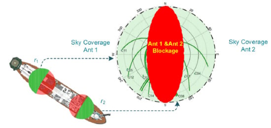
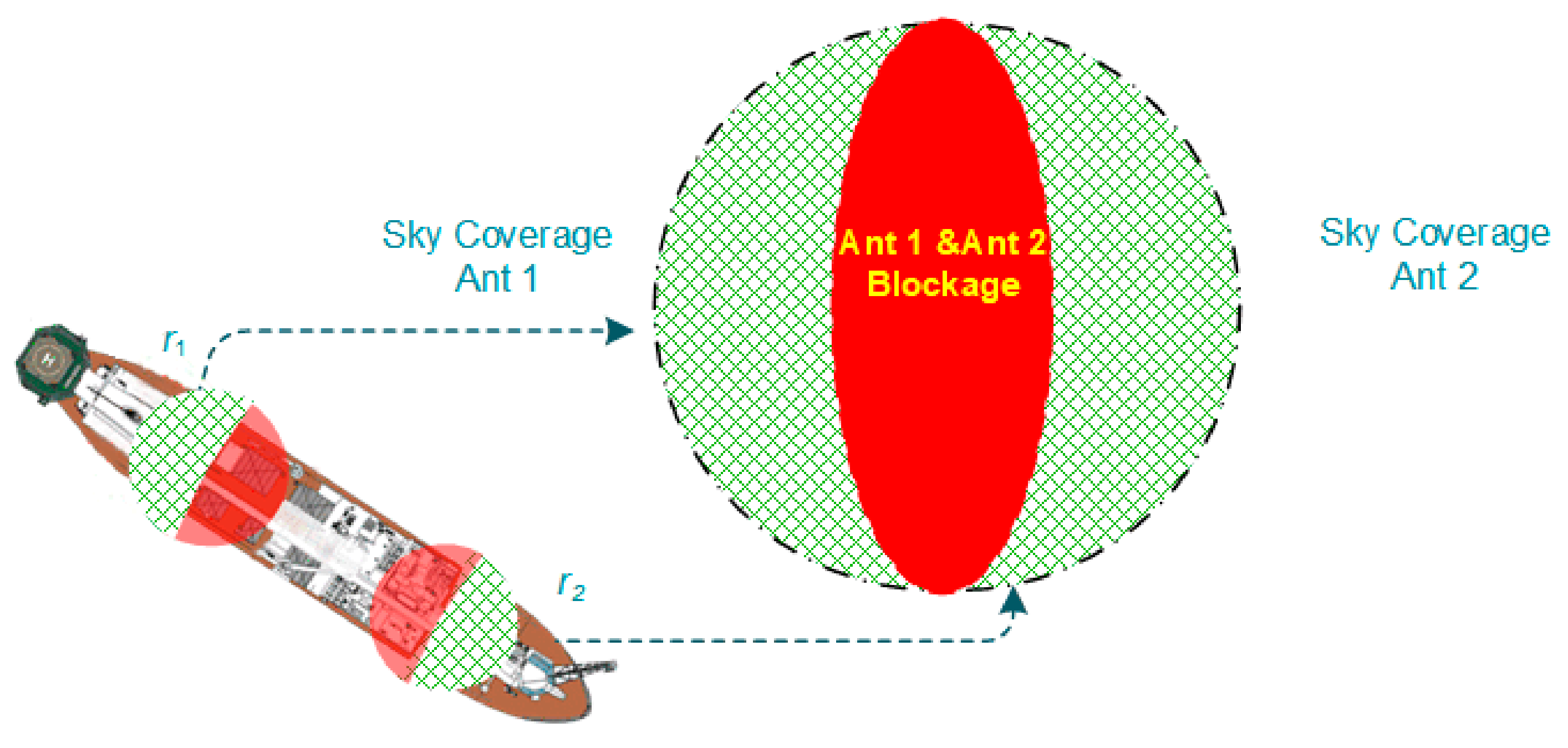
The relative positioning of moving platforms derived by the real-time kinematic (RTK) often suffers from satellite obstruction and deprived satellite visibility, which is especially true for offshore loading operations. This situation is often experienced on vessels working close to offshore platforms or other shadowing objects (e.g., island structure), where the field view of antenna is continuously varying and different satellite signals will be temporally blocked, as shown by the typical marine positioning applications in Figure 1. It is imperative that at least four satellites must be common-in-view at both rover and reference receivers. However, the traditional RTK usually implements high precision positioning with a single rover receiver [1]. In the worst case, the common-in-view satellites between the rover and the reference are insufficient to provide enough observations to enable the integer ambiguity resolution [2,3,4]. Additionally, some observations are possibly corrupted by multipath, so that more measurements than usually are necessary to strengthen the relative positioning. To overcome this issue, one solution is taking advantage of the multi-constellation to increase the number of satellites in view [5,6], whose benefits are demonstrated in case of weakly obstructed conditions, but degrade likewise under the severely satellite-limited environments. The other solution is to deploy multiple receivers, exploring more available observations to improve ambiguity resolution and positioning accuracy under the satellite-deprived environments [7,8,9].
The multiple receivers-based positioning method is a generalized measurement concept in RTK and precise point positioning (PPP) or PPP-RTK, which uses global navigation satellite system (GNSS) data from multiple antennas to realize improved GNSS parameter estimation [10,11]. Its applications have been widely extended in the fields of deformation monitoring [12], flight formation [13], attitude determination [7,14], bias, and ionosphere sensing [15,16]. The involved approaches of improving the model strength or estimation accuracy are to combine common-in-view satellites’ observations among those available receivers. Whereas under the constrained environment, particularly when there are various observational occlusions for the receivers, the decreased number of common-in-view satellites for those receivers will similarly weaken model strength relative to the conventional multiple receivers RTK positioning method. Therefore, it is necessary to tightly integrate the observations from all receivers and improve the strength of the positioning model, so as to ensure the ambiguity resolution and the continuity of the RTK positioning method under the restricted navigation environment [17]. Hence, we propose employing few mounted antennas with corresponding, individual receivers on a platform and combine their observations into a common set that has enough information to estimate an accurate position. Thus, the effect of obstructions on relative positioning can be released. Related research has demonstrated that increased precision in terms of dilution of precision (DOP) is obtained, and continuity can be guaranteed in the positioning [18].
Generally, owing to the sky blockage, different antennas may have access to different sets of satellite signals, and there are two strategies to deal with different available satellites among those receivers to improve the field view when constructing double-differenced (DD) observations [17,19]. The first strategy is that each rover receiver selects its own pivot satellite with respect to the reference receiver individually [19,20], but the introduction of multiple pivot satellites will reduce the redundancy of observation model. The other strategy is to fix the pivot satellite relative to the reference receiver in order to enhance the observation redundancy. However, when the clocks origination between each rover receiver are independent of each other, the receiver hardware delay related biases and the receiver clock errors are different from each other, which will yield inter-receiver bias (IRB) in the double-differenced observations. IRB consists of inter-receiver hardware biases and inter-receiver clock error. When the rover receivers utilize independent clocks, the inter-receiver clock error is usually not stable and the IRB becomes a time-varying parameter to be estimated. In addition, the number of IRB parameters increases exponentially with the number of non-common clock-driven rover receivers [18], which reduces the redundancy of the DD observations. Consequently, multiple rover receivers under the common clock mode, i.e., the signals from multiple receivers are driven by a common clock, is a feasible approach to improve the redundancy of DD observations [21].
Multiple rover receivers sharing the common clock does not imply that the inter-receiver biases for each rover are identical [22]. It is because that the clock provides each rover receiver with only a stream of pulses without an absolute time tag. Therefore, due to the inconsistent transmission clock signal delays to those receivers when the receivers are powered on, the inter-receiver clock errors under the common clock mode will be time-varying [23]. Odijk and Teunissen [24], Paziewski and Wielgosz [25], and Zhang and Teunissen [26] have shown that inter-receiver hardware biases have time-domain stability, and its stability is affected by ambient temperature and so on, which can be regarded as a time-invariant to be pre-estimated and calibrated for eliminating the influence on ambiguity resolution [27]. Therefore, the common clock-induced IRB is anticipated to have a stable time-domain feature, which provides the foundation to perform calibration. In this contribution, the RTK positioning method with multiple rover receivers sharing the common clock (C-RTK) is investigated to calibrate the IRB by the pre-estimated correction strategy for suppressing the influence on the integer ambiguity resolution, thereby improving the strength of the observational model.
This contribution is structured as follows: taking the Beidou Navigation Satellite System (BDS) dual-frequency signal as an example, we formulate the RTK positioning method with multiple rover receivers sharing the common clock under short-baseline cases. Then, the IRB stability characteristics under the common clock mode and non-common clock mode are compared by three different datasets with non-common clocks and a set of BDS dual-frequency short baseline dataset. Additionally, by simulating the constrained environment, the performance of the proposed method is explored. At the last section, the corresponding conclusions are drawn.
2. Methodology
We describe the observation models of IRB-float and IRB-fixed for the C-RTK method, respectively. Specifically, the IRB-float method estimates the unknown IRB simultaneously with the baseline coordinates and DD ambiguities. While the IRB-fixed method corrects the IRB using available calibrations in which no unknowns at all for the IRB is estimated. Meanwhile, the statistical characterization of IRB is introduced, including inter-receiver code bias and inter-receiver phase bias, which is followed by the two-step calibration procedure to implement IRB correction for the inter-receiver DD observations. The last of this section comes up with the redundancy and solvability analysis for C-RTK method.
2.1. IRB-Float Model
To derive the methodology of IRB-float positioning model, it is necessary to briefly review the single-differenced (SD) observations between rover receivers “ri” and reference receivers “b”, in which the satellite-specific biases are eliminated. The SD phase and code observations are expressed as [28],
where , with i = 1, 2 and is the expectation operator, s = 1, …, n. The subscript j identifies a term associated with a frequency band. and denote the observed-minus-computed code and phase residual observations at frequency Bj, respectively. denotes a vector of non-dispersive terms including incremental receiver positions and zenith tropospheric delay with its design matrix . is SD ionospheric delay with the first order ionospheric coefficient . is the SD receiver clock error. and are SD receiver hardware delays with respect to code and phase observations. is SD integer ambiguity. Note that we focus on short-baseline applications for which the differential atmospheric delays are absent in the future derivation.
As shown in Figure 1, assuming that the satellites tracked by r1 are s = {1, 2, …, m}, and satellites tracked by r2 are q = {m + 1, m + 2, …, n}. With “classical” double differencing, we form double differences for per receiver pair, i.e., (r1, b) or (r2, b). For the receiver pair (r1, b), if we fix the pivot satellite as 1, the DD observations read,
Here, represents a double differencing operator. Similarly, provided m+1 as the pivot satellite for the receiver pair (r2, b), the DD observations read as,
where , with s = 2, …, m, q = m + 2, …, n. In order to benefit from the increased number of observations, we have to establish a common solution for the multiple rover receivers. With , we rewrite Equation (3) to construct the loosely coupled RTK using non-common clock (NC-RTK) method,
for q = m + 1, …, n. The implementation of (4) is the traditional RTK method, by which 2 satellites’ observations are decreased owing to DD operation with multiple pivot satellites.
The observation model in (4) is a relatively classical coupling to integrate observations from different rover receivers. When tight observation integration is considered for complementing the receiver pairs {(r1, b) and (r2, b)} SD observations, we construct the DD observations with respect to the common pivot satellite from the receiver pair (r1, b). Thus, the inter-receiver tightly coupled DD observations read,
where , with q = m + 1, …, n. Therefore, for the phase as well as code observations, one more DD observation can be obtained by (5) when compared with (4). On the other hand, the inter-receiver bias terms are not eliminated during double differencing,
where and are referred as inter-receiver phase bias (IRPB) and inter-receiver code bias (IRCB), respectively. Unfortunately, the inter-receiver tightly coupled model described by (5) is rank deficient. It is, therefore, impossible to simultaneously estimate the IRB parameters and the ambiguity by (5) owing to the linear correlation between and IRPB. The rank deficiency is of size f (equal to the number of frequencies). Hence, we re-parametrize as,
Furthermore, we select as reference ambiguity to re-parametrize the inter-receiver DD ambiguity . The DD ambiguities relative to the same receiver pair, i.e., , plus inter-receiver ambiguity between the pivot satellite belonged to different receiver pairs, i.e., . The ambiguity is lumped to the IRPB term as,
We substitute (8) into (5), the full-rank IRB-float model can be expressed as,
in which denotes Kronecker product. D[·] is dispersion operator. is the DD phase observation vector with . is the DD code observation vector with . is f×1 vector of 1’s. A is the design matrix. with being the wavelength on frequency j. with 0 being m − 1 of 0’s vector and 1 being n − m + 1 vector of 1’s. x denotes the baseline vector. , . a is the DD ambiguity vector. and are covariance of DD phase and DD code, respectively. When n ≥ 5, and can be resolved by (9) with the dual-frequency single-system observations. However, when compared with the NC-RTK method as shown by (4), the increased number of observations for the IRB-float model is counter-balanced by the parameters to be estimated, which indicates the model strength of the IRB-float model is equivalent to the traditional NC-RTK method.
2.2. IRB-Fixed Model
It has been shown that if we parameterize the IRB for inter-receiver observations, it does not strengthen the model relative to NC-RTK method using the classical double differencing. However, the observation redundancy can still be retrieved if the statistical knowledge of the IRB can be provided [24]. For instance, given the stable statistical characteristics of the IRB, the observation redundancy can be obtained by a two-step method, i.e., the pre-estimation and post-calibration sequentially. Otherwise, if the IRB behaves without stationary statistical characteristics, then the IRB need to be estimated epoch-wisely. Correspondingly, the number of increased DD observations is equal to the number of additional parameters to be estimated, which takes no improvement on the DD observation redundancy. There is no doubt that the statistical characteristics of IRB determine the compensation strategy of IRB.
We can decompose the IRB term in the IRB-float model into two parts, the first part being an initial bias and the second part being the drift over time. Driving both rover receivers with a common clock only retains the identical second part for all rover receivers. Therefore, the IRB are treated as time-invariant terms instead of time-varying parameters, which are deterministic to be subtracted from the phase and code observations. The IRB-float model can be used to solve and . However, we can see from (8) that is biased by . This will be an issue for the IRB calibration when the pivot satellite change or in the presence of cycle slip. In order to avoid this issue, we separate into integral part and fractional part, respectively.
Obviously, the integral part of can be merged with ambiguity ,
Fortunately, the ambiguity retains the integer nature, which has no impact on instantaneous ambiguity resolution. However, when the factional part of (10) is not calibrated, it will undermine the ambiguity resolution success rate performance. Herein, in order to resolve the ambiguity, consideration should be taken into eliminating the factional part subsequently. Firstly, through removing the integer of IRPB by the nearest rounding method, the fractional calibration reads,
where round[·] is rounding to the nearest integer estimator. denotes the estimation of . The following experimental results will prove the time-domain stability feature of the IRB. As a result, IRB can be corrected by pre-calibration. On the basis of (12), the IRB-fixed model can be given as,
When the IRB is calibrated, the above full-rank model will regress to the traditional RTK positioning model. From this follows the important conclusion that when the inter-receiver biases are corrected (2f corrections), the fused observations from each receiver pair can be processed as if they were stemmed from one common receiver pair. The model strength is improved ultimately, which is further clarified in Section 3.
3. Redundancy and Solvability Analysis
Provided that there are k + 1 rover receivers tracking n satellites simultaneously, Table 1 gives the number of observations, the number of parameters, and the observation redundancy for different RTK models. It can be found that the IRB-float model is equivalent to the NC-RTK model. Compared with the IRB-float model, the unknown parameters amount of the IRB-fixed model is decreased by kf, which means that the strength of the observation model is further enhanced after IRB is eliminated.
4. Experimental Analysis and Discussion
To test the proposed method, a series of experiments were carried out. Firstly, we analyze and compare the stability of IRCB and IRPB under the common clock mode and the non-common clock mode, respectively. With different cut-off elevations, this contribution simulates the satellite-deprived environment. Because the short baseline data were collected, the atmospheric delays are neglected in the experimental data processing. Additionally, to analyze the ambiguity solution success rate and the positioning accuracy performance, the variants of two RTK algorithms compared in this contribution are NC-RTK and the C-RTK driven by the IRB-fixed model. Besides, assuming that multipath error is coupled with the thermal noise, the elevation-dependent weighting model is applied to account for the effect of multipath, and the observational standard deviation (STD) with elevation angle θ is set as , in which takes 30 cm and 3 mm for original code and phase observation, respectively [29,30]. Since in the short-baseline case most receiver-dependent and satellite-dependent errors are eliminated by DD operation, the instantaneous ambiguity resolution strategy is applied to the fix/float solutions. Herein, we utilize the metrics of success rate and the positioning accuracy to evaluate the fix and float solutions for the NC-RTK and C-RTK models. It has been widely proven that the LAMBDA algorithm performs excellent ambiguity resolution performance among the different integer aperture estimation methods [3]. We, therefore, apply LAMBDA to fix ambiguity, in which the threshold for the ratio test is set as 3 [31].
4.1. Receivers Setup
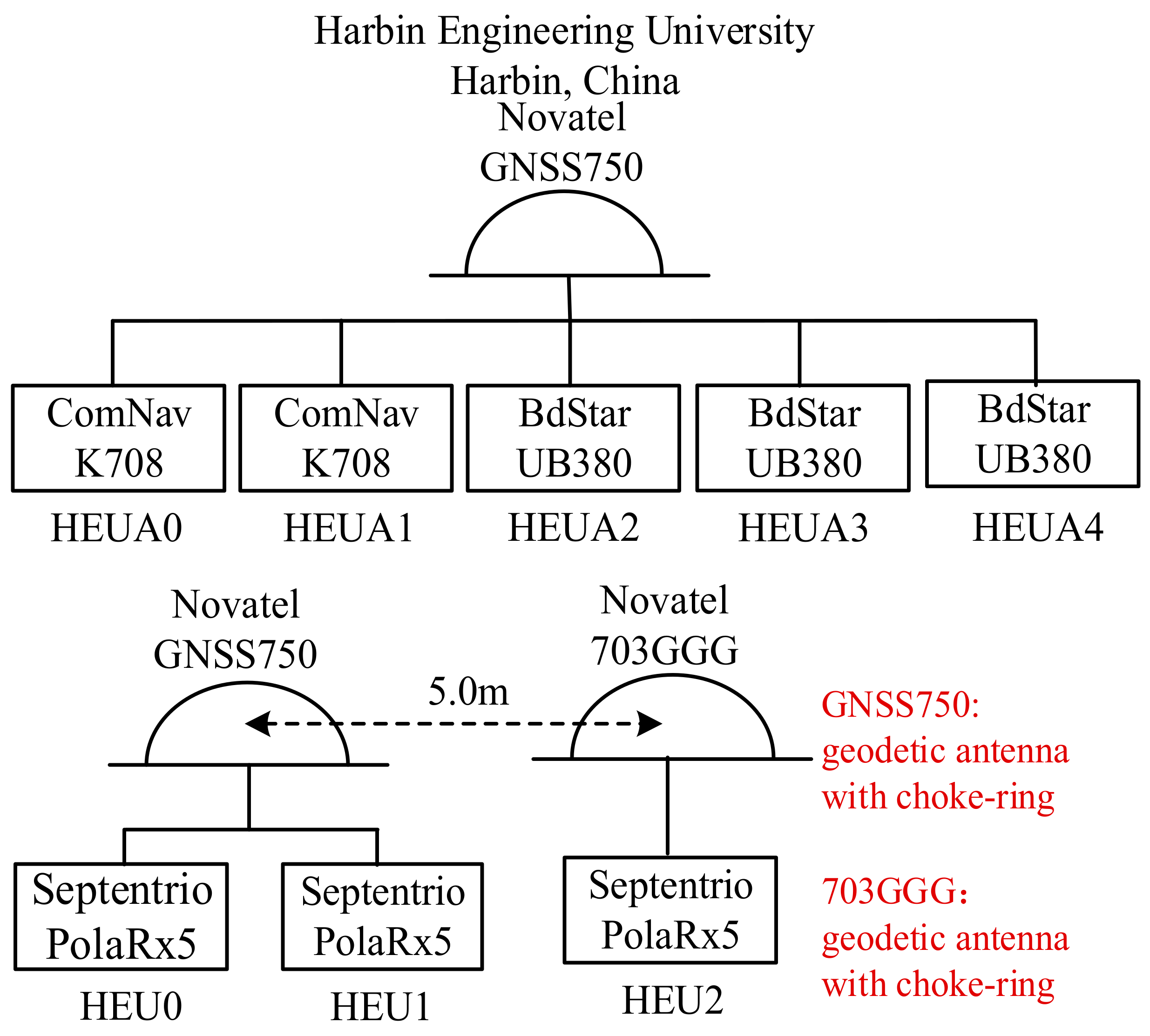
The experimental datasets were collected at Harbin Engineering University in China, where several high-grade receivers with geodetic antennas were setup under an open-sky environment to disentangle the multipath effect. The rover receivers are BDStar UB380 with non-common clocks, the ComNav K708 with non-common clocks, and the Septentrio PolaRx5 with an external common clock. Note that the time-frequency stability of the common clock for Septentrio PolaRx5 receivers is up to 10−11 level. The datasets we collected include dual-frequency BDS code and carrier phase measurements. IRB-float model is used to estimate the corresponding IRB sequences, by which the stability of IRB under the common clock and non-common modes are, respectively, analyzed during a 96-h time span and a 24-h time span. All receivers were installed in a room with a relatively constant ambient temperature, including HEUA0-HEUA4 and HEU0-HEU1 connected to one same antenna GNSS750. Therefore, we can form several different configurations of zero-baseline and short baseline. The schematic overview of all receivers and antennas involved is shown in Figure 2 and the detailed baseline configurations are listed in Table 2.
4.2. IRPB Estimation Results
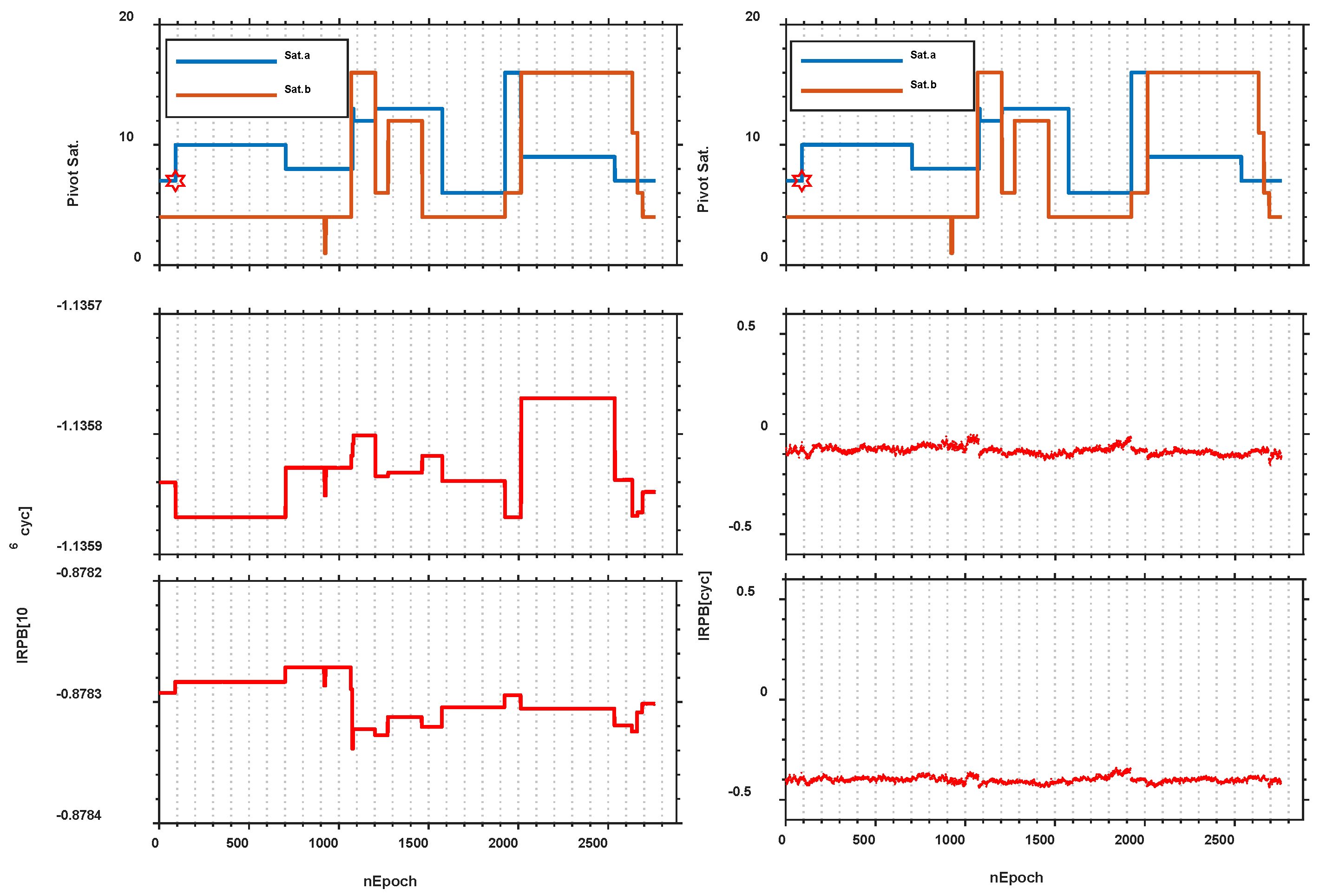
Considering a typical example, 24-h time series of epoch-wise IRPB estimated results are presented in Figure 3, which are determined by IRB-float model using BDS dataset collected with the short baseline {HEU0, HEU1}-HEU2 on day 160 of 2020. It can be found in Figure 3 that significant jumps ranging from several cycles during the 24 h continuous arc, which takes a detrimental effect on the acquisition of IRPB correction. It additionally confirms that each jump occurs immediately at the instant when the current pivot satellite sets and a new pivot satellite comes into view. Prior to our analysis, appropriate handling of these jumps should be taken. Therefore, the removal of integer part for the estimated IRPB results allows us to eliminate those jumps, resulting in the second panel time series that is jump-free. It can be used for further analysis without destroying the integer nature of ambiguity.
4.3. IRB Analysis under the Non-common Clock Mode
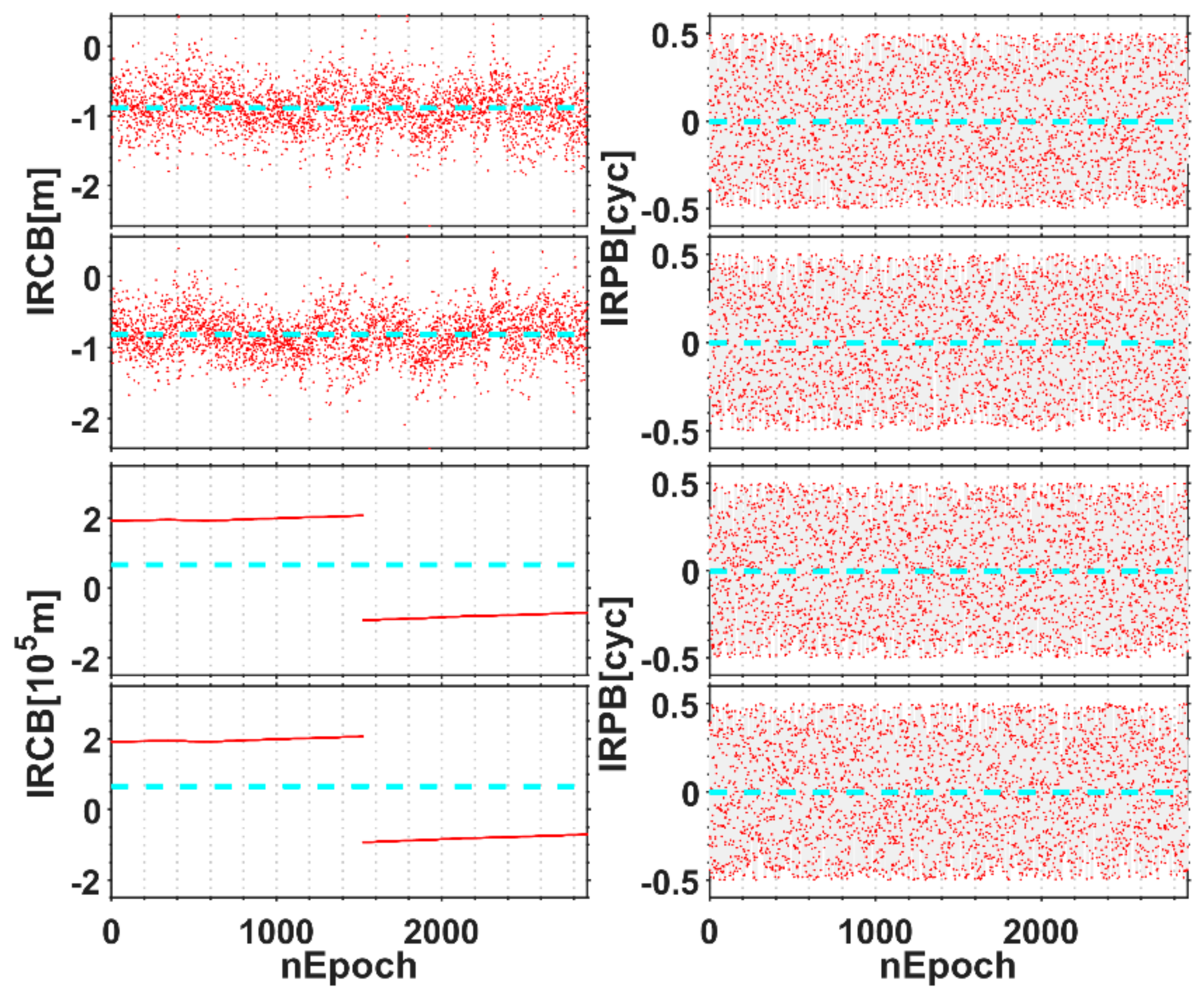
With the IRCB and IRPB estimated model, we obtain the epoch-wise results of IRB for UB380 and K708, in which the fractional part of IRPB is given in Figure 4. It can be found that the IRCB is not affected apparently by non-common clocks-based rover receivers. It is very stable in a 24-h observation span, making slight random fluctuations around its mean value. However, the fractional part of IRPB for B1 and B2 ranges from −0.5 to 0.5 cycles irregularly, whose STD reaches 0.3 cycles. Therefore, the IRB over the 24 h short-term temporal time series fluctuated too wildly to be calibrated in advance.
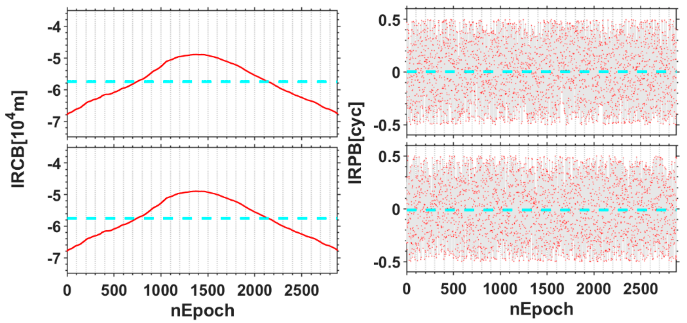
As shown by Figure 4, the IRCB estimation results for UB380 under non-common clock mode are not stable within the 24 h fixed arc and reach the order of 105m. In addition, IRB with respect to the carrier phase for the two frequencies also presents random fluctuations ranging from −0.5 to 0.5 cycles, which is difficult to be accurately modeled. Furthermore, at the 1500th epoch, the IRCB of both B1 and B2 frequency have obvious jump. It is because the internal clocks of UB380 receiver used in those two receivers are independent quartz clocks, in which the clock errors for two rover receivers will gradually drift. Generally, when the clock errors of the receiver exceed a certain threshold, the clock jump will be inserted for reset control to keep its accuracy within a certain range. However, for the case of non-common clock mode, the clocks of independent receivers are inconsistent owing to asynchronous processing strategies by two independent rover receivers. Hence, the jump phenomenon as shown in Figure 4 is present. However, it is noted that the phenomenon might not necessarily appear owing to asynchronous characteristics of random for every rover receiver clock. We collected another data using three UB380 receivers with non-common clocks on DOY148, 2019. Figure 5 shows that the clock jump is not present but with a trend item because the practical clock drifts for the rover receivers are neither common nor up to the level to reset control. In conclusion, the IRB under the non-common clock mode is not stable, which has shown that the pre-estimated correction method cannot be applied to calibrate the non-common clock-based IRB (Table 3).
4.4. Characterization of IRB under the Common Clock Mode
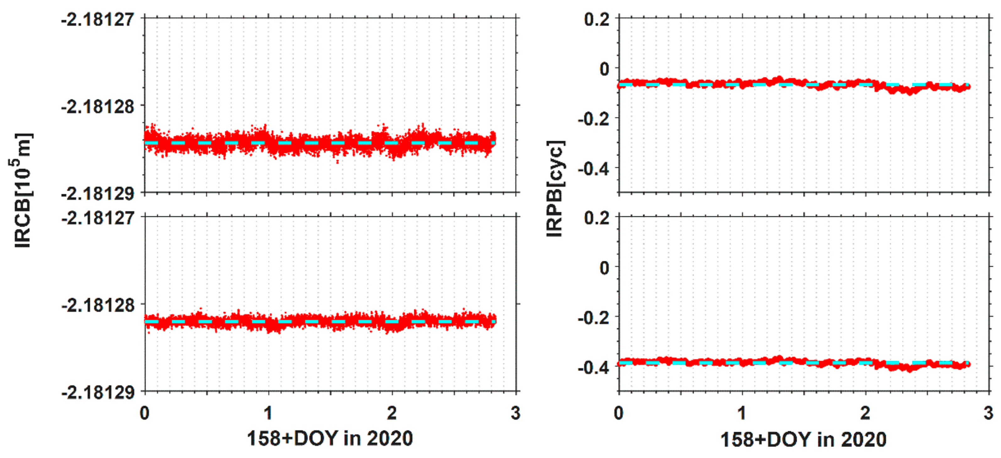
The time-domain stability of IRB is the key for C-RTK method to improve the strength of the positioning model. Therefore, this contribution spares more attention on analyzing the stability of IRB under the common clock mode. Firstly, the IRB-float model is utilized to estimate the IRCB and IRPB sequences, and the corresponding IRB results are shown in Figure 6.
Figure 6 depicts that the IRCB at B1 and B2 frequency reach the order of magnitude of 105 m with slight fluctuation near the mean value. The standard deviations corresponding to B1 and B2 frequencies are 0.28 m and 0.22 m, respectively, which reflect the statistical stability of IRCB. In addition, it can also be seen from Figure 6 that the IRPB for B1 and B2 frequency is also relatively stable because the standard deviations reach 0.021 cycles and 0.015 cycles for B1 and B2, respectively, which has no influence on the ambiguity resolution. Therefore, with the common clock mode, the averaging IRB estimation results over multiple epochs can be used as the calibration for the ambiguity resolution.
Previous studies have shown that the stability of IRCB and IRPB can be affected by a restart of the receiver and temperature fluctuation of the hardware [22,26]. Since our datasets are collected indoor environment with nearly constant temperature, therefore, the effect of temperature fluctuation on the IRB will not be considered in this contribution. Herein, we only test whether the stability of the IRCB and the IRPB are affected by the receiver restart. Additional datasets are collected by {HEU0, HEU1}-HUA2 at Harbin, China, for 4 days from DOY 153, 2020 with the sampling period of 30 s, in which the restart of the receiver will be executed about every 24 h for three times. The IRCB and the IRPB estimation results are shown in Figure 7. It can be seen that the fluctuation of IRPB caused by the receiver’s restart may be significantly larger than the phase observational noise. Similarly, the jumps are presented for IRCB estimated results that dramatically outweigh a lot before and after reboot, which implies that it is impossible to be calibrated by one same correction. Therefore, the IRCB and IRPB should be re-calibrated in IRB-fixed model when the receiver is restarted.
4.5. Performance of the IRB-Fixed Model
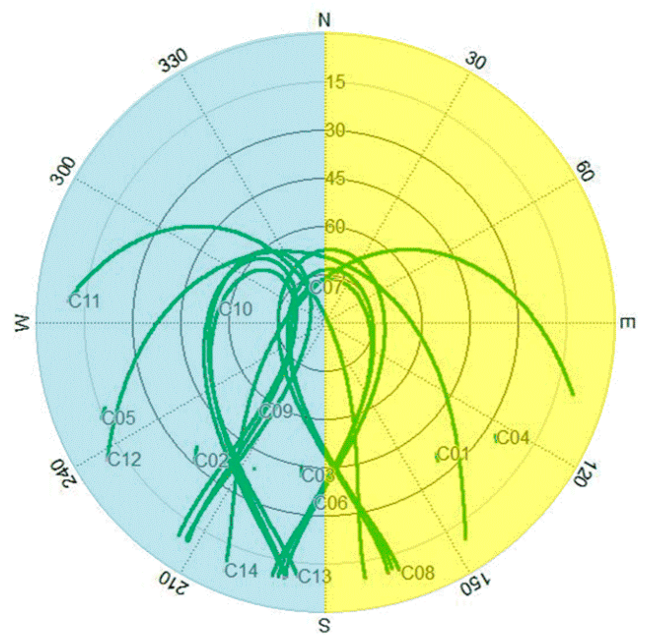
In order to evaluate the advantages of the proposed method over the traditional NC-RTK method in terms of positioning accuracy and integer ambiguity resolution, we simulate the obstructed satellite visibility cases. In this section, an experiment was conducted with three PolaRx5 on DOY158, in which two receivers, indicated as r1 and r2, were equipped with a common clock and a common antenna. Moreover, the third receiver as the reference receiver, denoted as b, has a 5 m baseline distance with the other two receivers. The sky plot of all tracked BDS satellites for r1 and r2 is given in Figure 8. In order to simulate the constrained environment, firstly, we manipulate the available satellites for r1 are corresponding to the azimuths ranging from 180° to 360°, the available satellites for r2 are from 0° to 180°. Therefore, the extreme case that there are no common-in-view satellites between rover can be created. Secondly, the elevation mask θ is adjusted from 10° to 30° for all the receivers with step of 5°. Thirdly, the azimuth mask α for r1 and r2 with the step of 10° is decreased to create less available satellites between rover receivers. The satellite constrained environment may also introduce multipath and sometimes other types of interference that are not considered in this contribution. We use the ambiguity dilution of precision (ADOP) and position dilution of precision (PDOP) to show the benefit of more observation redundancy from utilizing the proposed method [32]. The mean values of the estimated IRCB and IRPB sequences listed in Table 4 are used as a correction to calibrate the IRB for the second baseline configuration with a common clock. The empirical success rate Ps for ambiguity resolution is defined as the ratio between the correctly-fixed epochs and the total epochs.
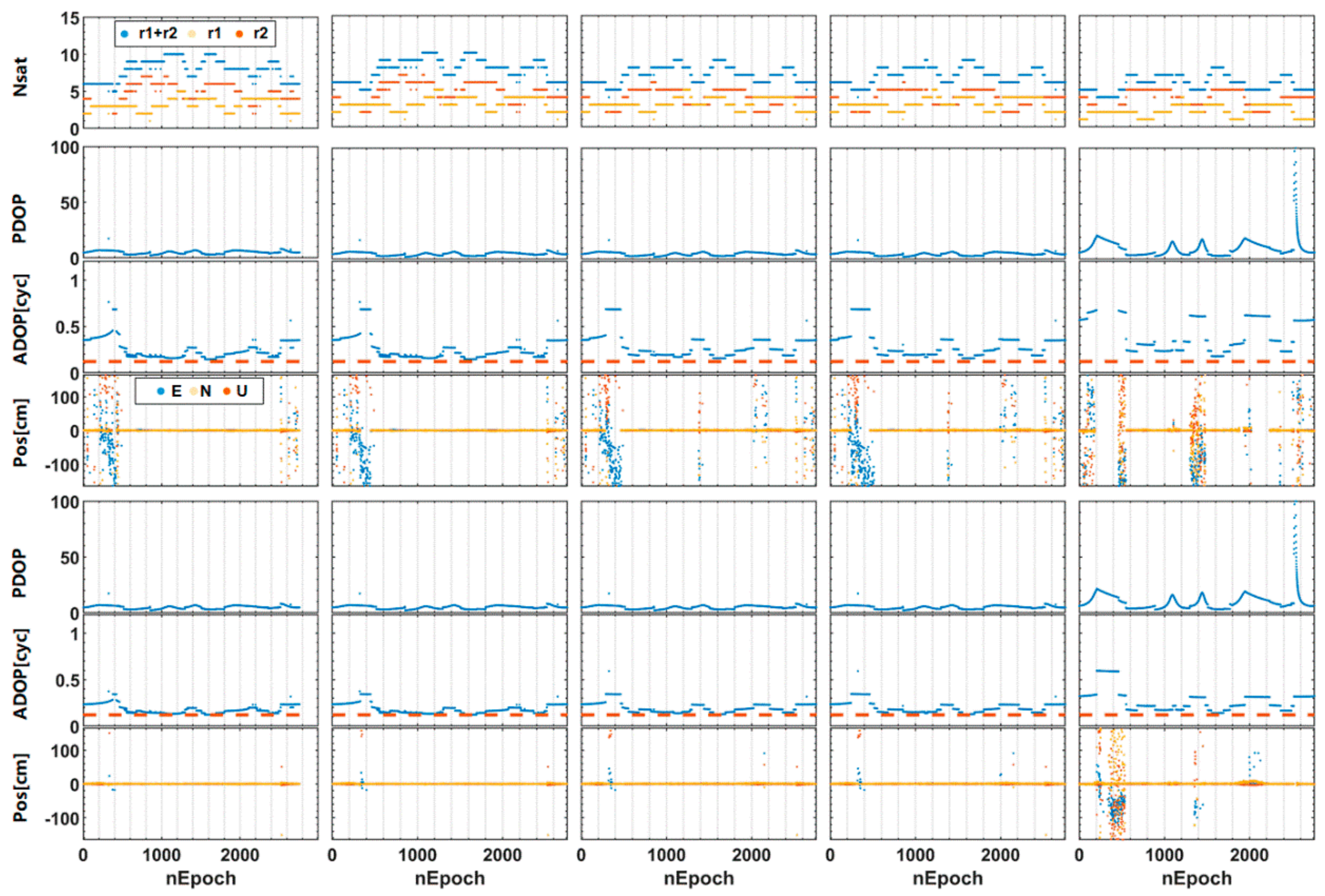
Figure 9 gives the positioning results, including the fixed solutions and float solutions. The statistical results are summarized in Table 5, including the root mean square (RMS) of 3D positioning errors and the success rate of ambiguity resolution. Note that Figure 9 only shows the worst case of all the experimental results, only a fraction of epochs was processed due to either the insufficient satellites for positioning or extremely poor satellite geometry (PDOP>30) under the BDS-only situation. Furthermore, it can be observed from Figure 9 that when the azimuth masks for r2 and r1 are up to (160°, 200°), the NC-RTK has more positioning interruptions due to the number of satellites are required at least five for the traditional RTK method. In contrast, the C-RTK method has better continuity performance because of the observation redundancy from IRB calibration.
When the sky blockage is not severe (e.g., the azimuth masks for r2 and r1 are all 180°, and the cutoff elevation is less than 25°), the performance of the C-RTK is comparative to NC-RTK. Because in the open sky scenario spliced jointly by r1 and r2, the C-RTK method can rarely improve DOP values and there are sufficient numbers of satellites to fix the ambiguity. However, this situation will change with the decrease of satellites in view. As shown in Figure 9, the C-RTK method has better ADOP relative to NC-RTK, which is further validated by the ambiguity resolution success rate. In addition, Figure 9 shows that the incorrectly fixed cases are present when the ADOPs are significantly more than the 0.12 cycle level. When the cutoff elevation angle is set to less than 20°, it can be seen from Table 5 that the integer ambiguity resolution and positioning performance of C-RTK are better with closely Ps of 99.5%, and the positioning accuracy within 30 cm. The results indicate that the proposed method is comparable with the traditional NC-RTK method since the advantages of additional observations remain tiny for the two methods under the open-sky environments. Furthermore, we find that the C-RTK behaves better in the satellite-deprived environment. Particularly, when the cutoff elevation is increased up to 30°, the integer ambiguity resolution and positioning performance for the NC-RTK method are much worse than the proposed C-RTK method. Specifically, the success rate of the NC-RTK method decreases by 27.17%, and the positioning accuracy is up to the meter level. Correspondingly, the success rate of C-RTK method decreases by 7.68%. Nevertheless, compared with NC-RTK method, the C-RTK method improves success rate by 19.5% and positioning accuracy by 46.4%. It is because the averaging of IRB as the correction to calibrate bias sequences will not affect the integer ambiguity resolution. In addition, the C-RTK method has more redundancy over the NC-RTK when the averaged IRB is used to calibrate inter-receiver DD observations. A slightly better ADOP can be obtained due to the increased observation redundancy. Therefore, the better ambiguity resolution success rate and the positioning accuracy of C-RTK can be achieved under the satellite-deprived environment owing to stronger observation model strength.
5. Concluding Remarks
To improve the integer ambiguity resolution and positioning performance under the satellite-deprived environments, we developed an RTK positioning method with multiple rover receivers sharing common clock. The proposed method can improve the observation redundancy by integrating the observations from multiple rover receivers. Regarding the code and phase IRB resulting from the integrating multiple rover receivers, a code and phase IRB estimation method is investigated, in which the phase IRB estimation is immune to the cycle slip or the change of pivot satellite. Fortunately, the experimental results have shown that the standard deviation of the carrier phase IRB under the common clock mode is less than 0.1 cycles. We, therefore, can use the pre-estimation-based IRB calibration strategy for the tightly integrating multiple rover receivers. However, the stability of code IRB and phase IRB can be destroyed by the reboot of the receiver, which implies that it is necessary to re-calibrate the IRB when the receiver is restarted.
Real-world datasets have demonstrated that, because of the stronger observation strength obtained by calibrating IRB, the proposed tightly coupled C-RTK method can obtain a higher positioning accuracy and ambiguity resolution performance achievement relative to the traditional loosely coupled NC-RTK method when under the short baseline satellite-deprived environment. It should be noted that we only compare the short baseline application in mild multipath and homothermal environment. Further study will be developed to investigate the temperature sensitivity of IRB and the multipath effect on the proposed method.
Author Contributions
Conceptualization, L.Z. and J.J.; methodology, L.Z.; validation, J.J., L.L. and C.J.; formal analysis, J.J.; investigation, J.J.; resources, J.C.; data curation, J.J.; writing—original draft preparation, J.J.; writing—review and editing, J.J.; visualization, C.J.; supervision, C.J.; project administration, J.J. and C.J.; funding acquisition, L.Z., J.C. and L.L. All authors have read and agreed to the published version of the manuscript.
Funding
This research was jointly funded by the National Natural Science Foundation of China (Nos. 61773132, 61633008, 61803115, 62003109), the National Key Research and Development Program (No. 2017YFE0131400), the 145 High-tech Ship Innovation Project sponsored by the Chinese Ministry of Industry and Information Technology, the Heilongjiang Province Research Science Fund for Excellent Young Scholars (No. YQ2020F009), the Heilongjiang Province Research Science Fund for Distinguished Young Scholars (No. JC2018019), and the Fundamental Research Funds for Central Universities (Nos. 3072019CF0401, 3072020CFJ0402, 3072020CFT0403).
Institutional Review Board Statement
Not applicable.
Informed Consent Statement
Not applicable.
Data Availability Statement
The datasets that support the findings of this study are available from the author (J.J.) upon a reasonable request.
Acknowledgments
The authors would like to appreciate Haihui Xu for data collection.
Conflicts of Interest
The authors declare that they have no known competing financial interests or personal relationships that could have appeared to influence the work reported in this paper.
References
- Li, B.; Teunissen, P.J.G. Array-Aided CORS Network Ambiguity Resolution; Springer: Berlin/Heidelberg, Germany, 2014; pp. 599–605. [Google Scholar]
- Li, B.; Teunissen, P.J.G. Real-Time Kinematic positioning using fused data from multiple GNSS antennas. In Proceedings of the 2012 15th International Conference on Information Fusion, Singapore, 9–12 July 2012; pp. 933–938. [Google Scholar]
- Teunissen, P.J.G. The least-squares ambiguity decorrelation adjustment: A method for fast GPS integer ambiguity estimation. J. Geod. 1995, 70, 65–82. [Google Scholar] [CrossRef]
- Li, L.; Jia, C.; Zhao, L.; Yang, F.; Li, Z. Integrity monitoring-based ambiguity validation for triple-carrier ambiguity resolution. Gps Solut. 2017, 21, 797–810. [Google Scholar] [CrossRef]
- Borio, D.; Gioia, C. Galileo: The Added Value for Integrity in Harsh Environments. Sensors 2016, 16, 111. [Google Scholar] [CrossRef] [Green Version]
- Bitter, M.; Feuerle, T.; von Wulfen, B.; Steen, M.; Hecker, P. Testbed for Dual-Constellation GBAS Concepts. In Proceedings of the 2010 IEEE-Ion Position Location and Navigation Symposium Plans, Indian Wells, CA, USA, 4–6 May 2010; pp. 474–481. [Google Scholar]
- Giorgi, G.; Teunissen, P.J.G.; Verhagen, S.; Buist, P.J. Instantaneous Ambiguity Resolution in Global-Navigation-Satellite-System-Based Attitude Determination Applications: A Multivariate Constrained Approach. J. Guid. Control Dyn. 2012, 35, 51–67. [Google Scholar] [CrossRef]
- Paziewski, J. Precise GNSS single epoch positioning with multiple receiver configuration for medium-length baselines: Methodology and performance analysis. Meas. Sci. Technol. 2015, 26, 035002. [Google Scholar] [CrossRef]
- Li, H.; Gao, S.; Li, L.; Jia, C.; Zhao, L. Real Time Precise Relative Positioning with Moving Multiple Reference Receivers. Sensors 2018, 18, 2109. [Google Scholar] [CrossRef] [PubMed] [Green Version]
- Teunissen, P.J.G. A-PPP: Array-Aided Precise Point Positioning with Global Navigation Satellite Systems. IEEE Trans. Signal Process. 2012, 60, 2870–2881. [Google Scholar] [CrossRef]
- Li, W.; Nadarajah, N.; Teunissen, P.J.G.; Khodabandeh, A.; Chai, Y. Array-Aided Single-Frequency State-Space RTK with Combined GPS, Galileo, IRNSS, and QZSS L5/E5a Observations. J. Surv. Eng. 2017, 143, 04017006. [Google Scholar] [CrossRef]
- Chen, Y.; Ding, X.; Huang, D.; Zhu, J. A multi-antenna GPS system for local area deformation monitoring. Earth Planets Space 2000, 52, 873–876. [Google Scholar] [CrossRef] [Green Version]
- Buist, P.J.; Teunissen, P.J.G.; Giorgi, G.; Verhagen, S. Multivariate bootstrapped relative positioning of spacecraft using GPS L1/Galileo E1 signals. Adv. Space Res. 2011, 47, 770–785. [Google Scholar] [CrossRef]
- Li, N.; Zhao, L.; Li, L.; Jia, C. Integrity monitoring of high-accuracy GNSS-based attitude determination. Gps Solut. 2018, 22, 120. [Google Scholar] [CrossRef]
- Khodabandeh, A.; Teunissen, P.J.G. Array-based satellite phase bias sensing: Theory and GPS/BeiDou/QZSS results. Meas. Sci. Technol. 2014, 25, 095801. [Google Scholar] [CrossRef] [Green Version]
- Khodabandeh, A.; Teunissen, P.J.G. Array-Aided Multifrequency GNSS Ionospheric Sensing: Estimability and Precision Analysis. IEEE Trans. Geosci. Remote Sens. 2016, 54, 5895–5913. [Google Scholar] [CrossRef]
- Gioia, C.; Borio, D. Android positioning: From stand-alone to cooperative approaches. Appl. Geomat. 2020. [Google Scholar] [CrossRef]
- Kube, F.; Bischof, C.; Alpers, P.; Wallat, C.; Schön, S. A virtual receiver concept and its application to curved aircraft-landing procedures and advanced LEO positioning. Gps Solut. 2018, 22, 41. [Google Scholar] [CrossRef]
- Khanafseh, S.; Kempny, B.; Pervan, B. New Applications of Measurement Redundancy in High Performance Relative Navigation Systems for Aviation. In Proceedings of the 19th International Technical Meeting of the Satellite Division of the Institute of Navigation, Fort Worth, TX, USA, 26–29 September 2006; pp. 3024–3034. [Google Scholar]
- Khanafseh, S.M.; Pervan, B. Autonomous Airborne Refueling of Unmanned Air Vehicles Using the Global Positioning System. J. Aircr. 2007, 44, 1670–1682. [Google Scholar] [CrossRef]
- Wang, Z.; Chen, W.; Dong, D.; Wang, M.; Cai, M.; Yu, C.; Zheng, Z.; Liu, M. Multipath mitigation based on trend surface analysis applied to dual-antenna receiver with common clock. GPS Solut. 2019, 23, 104. [Google Scholar] [CrossRef]
- Keong, J.; Lachapelle, G. Heading and Pitch Determination Using GPS/GLONASS. GPS Solut. 2000, 3, 26–36. [Google Scholar] [CrossRef]
- Chen, W.; Yu, C.; Dong, D.; Cai, M.; Zhou, F.; Wang, Z.; Zhang, L.; Zheng, Z. Formal Uncertainty and Dispersion of Single and Double Difference Models for GNSS-Based Attitude Determination. Sensors 2017, 17, 408. [Google Scholar] [CrossRef] [PubMed] [Green Version]
- Odijk, D.; Teunissen, P.J.G. Characterization of between-receiver GPS-Galileo inter-system biases and their effect on mixed ambiguity resolution. GPS Solut. 2013, 17, 521–533. [Google Scholar] [CrossRef]
- Paziewski, J.; Wielgosz, P. Accounting for Galileo–GPS inter-system biases in precise satellite positioning. J. Geod. 2015, 89, 81–93. [Google Scholar] [CrossRef] [Green Version]
- Zhang, B.; Teunissen, P.J.G. Characterization of multi-GNSS between-receiver differential code biases using zero and short baselines. Sci. Bull. 2015, 60, 1840–1849. [Google Scholar] [CrossRef] [Green Version]
- Jia, C.; Zhao, L.; Li, L.; Lu, R. BDS triple-frequency tightly coupled short-baseline RTK method by calibrating the between-receiver inter-frequency biases. Sci. Sin. Terrae 2020. [Google Scholar] [CrossRef]
- Zhang, B.; Liu, T.; Yuan, Y. GPS receiver phase biases estimable in PPP-RTK networks: Dynamic characterization and impact analysis. J. Geod. 2018, 92, 659–674. [Google Scholar] [CrossRef]
- Eueler, H.-J.; Goad, C.C. On optimal filtering of GPS dual frequency observations without using orbit information. Bull. Géodésique 1991, 65, 130–143. [Google Scholar] [CrossRef]
- Li, L.; Li, Z.; Yuan, H.; Wang, L.; Hou, Y. Integrity monitoring-based ratio test for GNSS integer ambiguity validation. Gps Solut. 2016, 20, 573–585. [Google Scholar] [CrossRef] [Green Version]
- Li, L.; Shi, H.; Jia, C.; Cheng, J.; Li, H.; Zhao, L. Position-domain integrity risk-based ambiguity validation for the integer bootstrap estimator. GPS Solut 2018, 22, 39. [Google Scholar] [CrossRef]
- Verhagen, S.; Teunissen, P.J.G. Ambiguity resolution performance with GPS and BeiDou for LEO formation flying. Adv. Space Res. 2014, 54, 830–839. [Google Scholar] [CrossRef] [Green Version]
Figure 1.
Schematic scenario of two rover-receivers equipped platform, Ant 1 and Ant 2 denote antennas for rover receivers r1 and r2, respectively.
Figure 1.
Schematic scenario of two rover-receivers equipped platform, Ant 1 and Ant 2 denote antennas for rover receivers r1 and r2, respectively.

Figure 2.
Receivers and antennas setup.

Figure 3.
24 h-time series of estimation results with Septentrio PolaRx5 receivers. The panels from left to right are the inter-receiver phase bias (IRPB) before and after eliminating the jumps. The subplots from top to bottom correspond to pivot satellites visibility, IRPB at B1 and B2 frequency, respectively. The single differenced ambiguities belonged to Sat.a and Sat.b form the ambiguity Nab, which is coupled in the IRPB. As an example, the hexagram marker specifies the time to alter.

Figure 4.
Estimation results for inter-receiver code bias (IRCB) and IRPB under non-common clock mode. The panels from left to right are the IRB for UB380 receiver and K708 receiver. The subplots from top to bottom correspond to IRCB and IRPB at B1 and B2 frequency, and the blue-green dotted line is the corresponding mean of IRB.

Figure 5.
The estimation results for IRCB and IRPB under non-common clock mode. The receiver types are all UB380. The panels from top to bottom represent IRCB and IRPB at B1 and B2 frequency, and the blue-green dotted line is the corresponding mean of IRB.
Figure 5.
The estimation results for IRCB and IRPB under non-common clock mode. The receiver types are all UB380. The panels from top to bottom represent IRCB and IRPB at B1 and B2 frequency, and the blue-green dotted line is the corresponding mean of IRB.

Figure 6.
The estimation results of IRCB and IRPB under common clock mode. Each row corresponds to B1 and B2 frequency from top to bottom, and the blue-green dotted line is the corresponding mean of IRB.
Figure 6.
The estimation results of IRCB and IRPB under common clock mode. Each row corresponds to B1 and B2 frequency from top to bottom, and the blue-green dotted line is the corresponding mean of IRB.

Figure 7.
IRCB and IRPB estimation results once restart of the receiver. The panels from left to right represent IRCB and IRPB, whose rows from top to bottom denote B1 and B2, respectively.
Figure 7.
IRCB and IRPB estimation results once restart of the receiver. The panels from left to right represent IRCB and IRPB, whose rows from top to bottom denote B1 and B2, respectively.

Figure 8.
The sky-plot of r1 and r2. Various colors denote different satellite tracking situations in the simulation, respectively. The light blue area denotes that the satellite signal tracked by r1 and the yellow represents tracked signals for r2, respectively.
Figure 8.
The sky-plot of r1 and r2. Various colors denote different satellite tracking situations in the simulation, respectively. The light blue area denotes that the satellite signal tracked by r1 and the yellow represents tracked signals for r2, respectively.

Figure 9.
Positioning results with different cutoff elevation angles, in which r1 and r2 can track satellites whose azimuth masks are 200° and 160°. The column panels from left to right represent different cutoff elevation angles (10°, 15°, 20°, 25°, 30°), respectively. The row panels from top to bottom are tracked satellite numbers, PDOP, ADOP (the ADOP is depicted in blue color, the 0.12-cycles level as orange dash line), and errors conditioned on PDOP<30 in east-north-up direction for the RTK positioning method using non-common clock receivers (NC-RTK) and the RTK positioning method with multiple rover receivers sharing the common clock (C-RTK), respectively.


Table 1.
Model redundancy analysis.
| Model | NC-RTK Model | IRB-Float Model | IRB-Fixed Model |
|---|---|---|---|
| # of observations | 2f(n − k − 1) | 2f(n − 1) | 2f(n − 1) |
| # of parameters | f(n − k − 1) + 3 | f(n + k − 1) + 3 | f(n − 1) + 3 |
| Redundancy | f(n − k − 1) − 3 | f(n − k − 1) − 3 | f(n − 1) − 3 |
Table 2.
Baseline setup.
| No. | Reference | Rover | Signals | Interval(s) | Distance(m) | Observation Span |
|---|---|---|---|---|---|---|
| 1 | HEUA2 | HEUA0 | B1 B2 | 30 | 0 | DOY147, 2019 |
| HEUA1 | B1 B2 | 30 | 0 | |||
| 2 | HEU2 | HEU0 | B1 B2 | 30 | 5.0 | DOY153–156, 158–161, 2020 |
| HEU1 | B1 B2 | 30 | 5.0 | |||
| 3 | HEUA0 | HEUA2 | B1 B2 | 30 | 0 | DOY147, 2019 |
| HEUA3 | B1 B2 | 30 | 0 | |||
| 4 | HEUA4 | HEUA2 | B1 B2 | 30 | 0 | DOY148, 2019 |
| HEUA3 | B1 B2 | 30 | 0 |
Table 3.
IRB statistics results under non-common clock mode.
| Baseline | Fre | IRCB | IRPB | ||
| Mean (m) | STD (m) | Mean (Cycle) | STD (Cycle) | ||
| {HEUA0,HEUA1}-HEUA2 | B1 | −0.8725 | 0.3399 | 0.0045 | 0.30 |
| B2 | −0.8320 | 0.3249 | 0.0050 | 0.30 | |
| {HEUA2,HEUA3}-HEUA0 | B1 | 65,902.9 | 139,203.6 | 0.0067 | 0.29 |
| B2 | 65,902.5 | 139,203.7 | 0.0010 | 0.29 | |
| {HEUA2,HEUA3}-HEUA4 | B1 | −57,534.6 | 5843.1 | 0.0128 | 0.29 |
| B2 | −57,535.1 | 5843.2 | 0.0036 | 0.29 | |
Table 4.
IRB statistics under the common clock mode.
| Type | B1 | B2 | ||
|---|---|---|---|---|
| Mean | STD | Mean | STD | |
| IRCB (m) | −218,128.42 | 0.28 | −218,128.20 | 0.22 |
| IRPB (cycle) | −0.081 | 0.021 | −0.40 | 0.015 |
Table 5.
Positioning performance and ambiguity resolution success rates.
| α (deg) | θ (deg) | NC-RTK (cm) | C-RTK (cm) | ||||||
|---|---|---|---|---|---|---|---|---|---|
| σE,RMS | σN,RMS | σU,RMS | Ps | σE,RMS | σN,RMS | σU,RMS | Ps | ||
| (180,180) | 10 | 0.35 | 0.34 | 0.82 | 100% | 0.19 | 0.28 | 0.68 | 100% |
| 15 | 0.35 | 0.34 | 0.76 | 100% | 0.19 | 0.27 | 0.63 | 100% | |
| 20 | 0.31 | 2.40 | 2.51 | 99.96% | 0.24 | 0.33 | 0.92 | 100% | |
| 25 | 0.32 | 2.41 | 2.52 | 99.96% | 0.25 | 0.34 | 0.95 | 100% | |
| 30 | 8.97 | 10.09 | 25.01 | 98.2% | 0.35 | 0.44 | 1.28 | 100% | |
| (170,190) | 10 | 17.27 | 33.91 | 69.47 | 97.57% | 0.98 | 2.41 | 4.50 | 99.96% |
| 15 | 19.82 | 41.65 | 83.66 | 97.03% | 0.59 | 5.88 | 11.75 | 99.86% | |
| 20 | 21.93 | 45.97 | 92.03 | 95.62% | 0.13 | 9.3 | 18.49 | 99.67% | |
| 25 | 28.90 | 61.88 | 122.84 | 93.33% | 2.20 | 10.18 | 20.26 | 99.57% | |
| 30 | 29.52 | 34.72 | 83.48 | 82.5% | 14.48 | 31.78 | 51.81 | 95% | |
| (160,200) | 10 | 25.93 | 56.59 | 104.86 | 93.44% | 0.68 | 5.12 | 9.69 | 99.86% |
| 15 | 32.58 | 70.51 | 129.95 | 93.04% | 0.84 | 8.84 | 18.63 | 99.67% | |
| 20 | 37.84 | 78.22 | 143.88 | 90.29% | 2.20 | 10.23 | 20.46 | 99.52% | |
| 25 | 41.76 | 84.42 | 158.05 | 88.77% | 2.32 | 11.37 | 22.71 | 99.45% | |
| 30 | 51.61 | 56 | 114.76 | 72.83% | 16.69 | 34.64 | 61.61 | 92.32% | |
Publisher’s Note: MDPI stays neutral with regard to jurisdictional claims in published maps and institutional affiliations. |
© 2021 by the authors. Licensee MDPI, Basel, Switzerland. This article is an open access article distributed under the terms and conditions of the Creative Commons Attribution (CC BY) license (http://creativecommons.org/licenses/by/4.0/).
Share and Cite
MDPI and ACS Style
Zhao, L.; Jiang, J.; Li, L.; Jia, C.; Cheng, J. High-Accuracy Real-Time Kinematic Positioning with Multiple Rover Receivers Sharing Common Clock. Remote Sens. 2021, 13, 823. https://0-doi-org.brum.beds.ac.uk/10.3390/rs13040823
AMA Style
Zhao L, Jiang J, Li L, Jia C, Cheng J. High-Accuracy Real-Time Kinematic Positioning with Multiple Rover Receivers Sharing Common Clock. Remote Sensing. 2021; 13(4):823. https://0-doi-org.brum.beds.ac.uk/10.3390/rs13040823
Chicago/Turabian StyleZhao, Lin, Jiachang Jiang, Liang Li, Chun Jia, and Jianhua Cheng. 2021. "High-Accuracy Real-Time Kinematic Positioning with Multiple Rover Receivers Sharing Common Clock" Remote Sensing 13, no. 4: 823. https://0-doi-org.brum.beds.ac.uk/10.3390/rs13040823
Note that from the first issue of 2016, this journal uses article numbers instead of page numbers. See further details here.