The SARSense Campaign: Air- and Space-Borne C- and L-Band SAR for the Analysis of Soil and Plant Parameters in Agriculture

Abstract

With the upcoming L-band Synthetic Aperture Radar (SAR) satellite mission Radar Observing System for Europe L-band SAR (ROSE-L) and its integration into existing C-band satellite missions such as Sentinel-1, multi-frequency SAR observations with high temporal and spatial resolution will become available. The SARSense campaign was conducted between June and August 2019 to investigate the potential for estimating soil and plant parameters at the agricultural test site in Selhausen (Germany). It included C- and L-band air- and space-borne observations accompanied by extensive in situ soil and plant sampling as well as unmanned aerial system (UAS) based multispectral and thermal infrared measurements. In this regard, we introduce a new publicly available SAR data set and present the first analysis of C- and L-band co- and cross-polarized backscattering signals regarding their sensitivity to soil and plant parameters. Results indicate that a multi-frequency approach is relevant to disentangle soil and plant contributions to the SAR signal and to identify specific scattering mechanisms associated with the characteristics of different crop type, especially for root crops and cereals.

1. Introduction

With the increasing impact of human activities and the effects of climate change on hydrological systems worldwide, appropriate and adapted management and mitigation concepts are required [1,2,3,4]. This is particularly true with regard to the goal of using natural resources more effectively and sustainably in the future [5]. Since soil moisture and water-related vegetation conditions are key parameters in this context, they need to be assessed and monitored at both global and local scales. By providing global data with high temporal and spatial resolution, modern Earth Observation (EO) satellites have become a key technology in this field, whose importance will significantly increase in the future [6,7,8].

Radar Observing System for Europe L-band SAR (ROSE-L), as one of the Copernicus High Priority Candidate satellite missions is foreseen to be able to target the abovementioned objectives. The mission was first agreed on at the European Space Agency (ESA) ministerial conference Space19+ in Seville in November 2019 and was contractually signed by ESA and Thales Alenia Space later in December 2020 as part of the Fourth ESA Copernicus Space Component Program. With a scheduled launch in 2028, the two satellites, carrying a quad-polarimetric L-band SAR, are designed for collecting valuable data, especially for various research and applications in the field of soil moisture, land cover mapping, maritime surveillance, and natural and anthropogenic hazards [9]. A third add-on satellite is currently under discussion for bi-static records (ROSE-L+). In synergy with the existing Sentinel-1 A/B SAR mission, ROSE-L will enhance the European radar imaging capacity by increasing the frequency of successive radar data collections. In this regard, it will also enhance the possibilities for using soil and plant parameter retrieval based on change detection methods (e.g., alpha approximation and interferometry methods). Since L-band wavelength is able to penetrate through various media like vegetation or dry snow, it additionally provides unique information that cannot be obtained using higher frequency bands like the Sentinel-1 C-band and vice versa [10,11,12]. In combination, a quasi multi-band space-borne radar product can be obtained, which is currently only available using individual airborne flight campaigns [9]. The joint NASA-ISRO SAR (NISAR) satellite mission planned by NASA and Indian Space Research Organization (ISRO) for 2022 can be seen as a potential precursor, carrying both an L- and S-band SAR [13]. In the course of the planning phase of the ROSE-L satellite mission, the potential of L-band SAR data for the proposed applications and the synergy effects from combining L- and C-band SAR data need to be explored. Such information will help to optimize ROSE-L regarding its synergies with the Sentinel-1 mission as well as with other radar satellite missions, e.g., RADARSAT Constellation Mission (RCM), NISAR, Advanced Land Observing Satellite (ALOS-2/4), Satélite Argentino de Observación con Microondas (SAOCOM), TerraSAR-X/TanDEM-X, Paz, and optical satellite missions, e.g., Sentinel-2 and the Landsat series.

Various flight campaigns were conducted in the past to unlock the information content of SAR data, particularly for measuring environmental parameters over agricultural and forested areas as

• The AgriSAR 2006 campaign was conducted over the Durable Environmental Multidisciplinary Monitoring Information Network (DEMMIN) agricultural site in Germany recorded C- and L-band SAR observations and multispectral images in preparation of Sentinel-1 and Sentinel-2 satellite missions [14].
• TropiSAR 2009 campaign was conducted over Nouragues, Paracou in French Guiana, with simultaneous P- and L-band SAR data recording, evaluating the potential of SAR for estimation of biomass over tropical forests [15].
• The Airborne Microwave Observatory of Subcanopy and Subsurface (AirMOSS) flight campaign was conducted between 2012 and 2015 using P-band SAR for polarimetric measurements over major North American biomes, especially focusing on root-zone soil moisture [16].
• The NASA-ISRO Airborne Synthetic Aperture Radar (ASAR) flight campaign in 2019 was conducted over different biomes in North America, investigating the potential of L- and S-band for environmental monitoring in the context of the upcoming NISAR satellite mission [17].
• The UAVSAR AM-PM campaign in 2019 was conducted over different biomes in the Southeastern United States in preparation for the upcoming NISAR satellite mission, using L-band SAR with alternating morning and evening acquisition times [18].

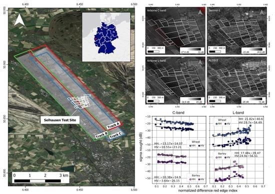
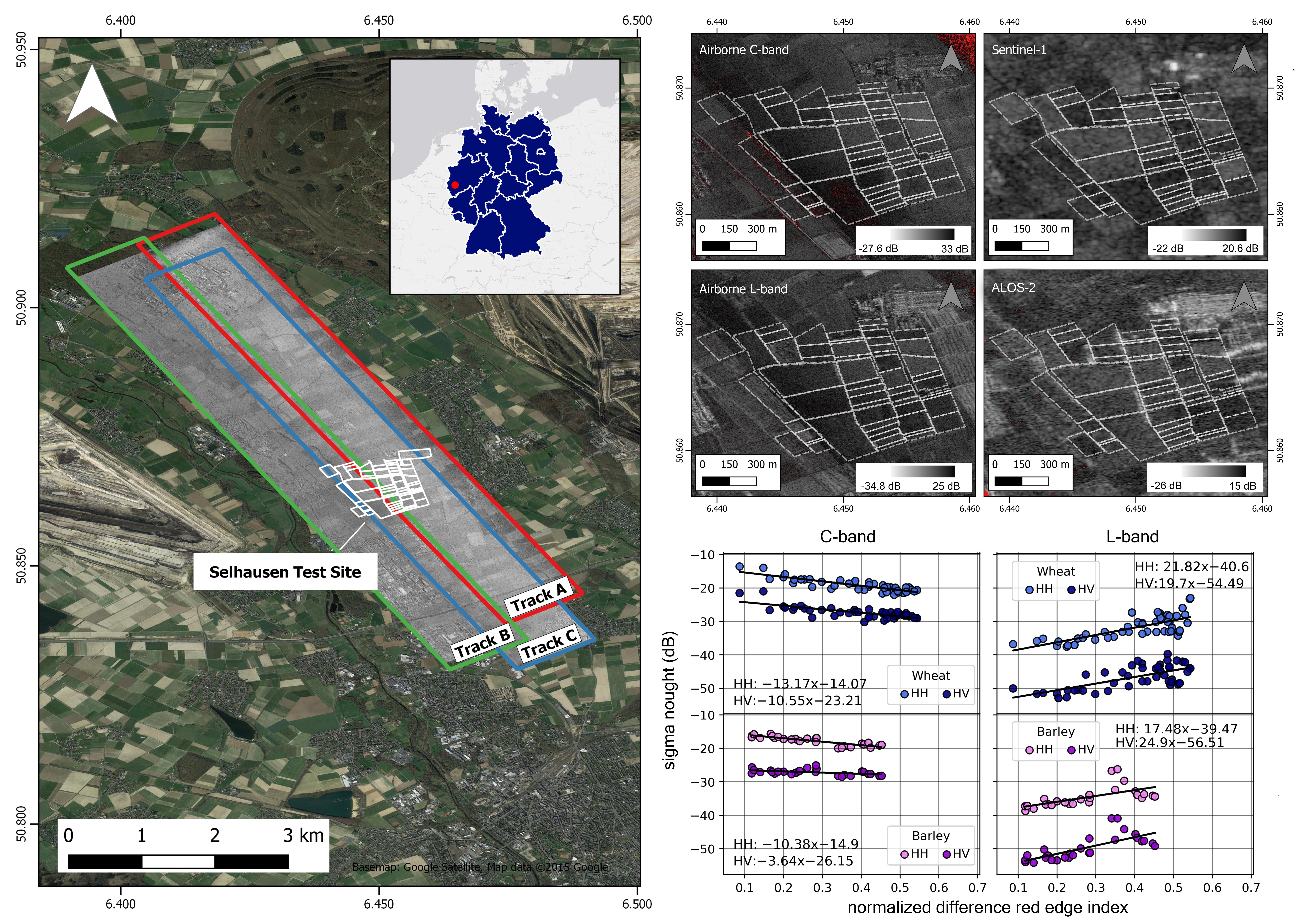
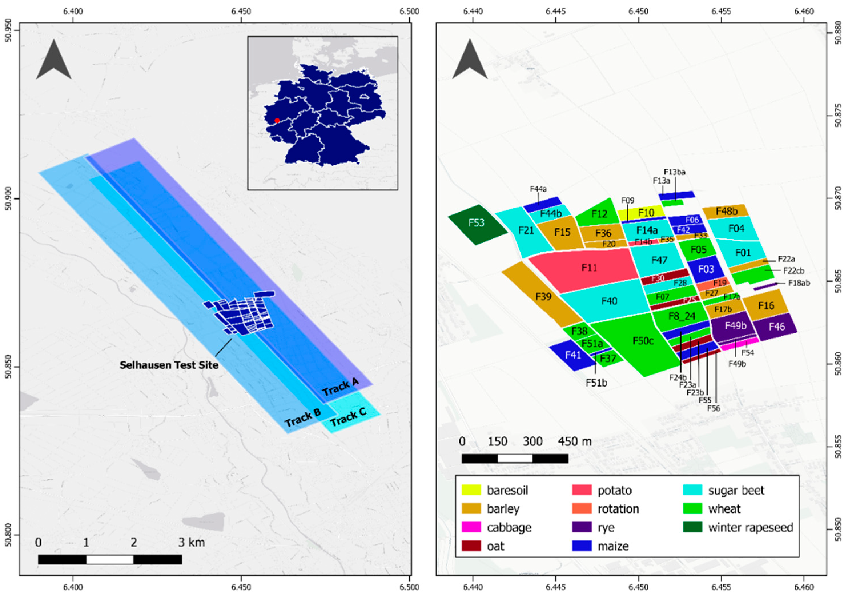
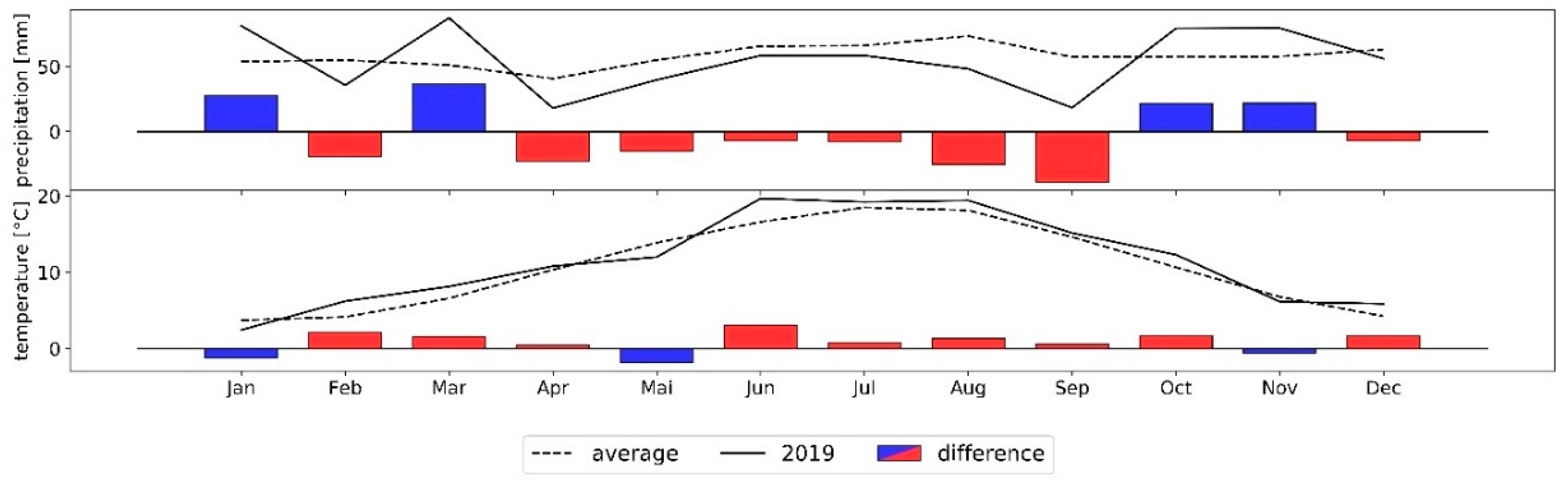
Soil moisture, being one of the key parameters within the hydrological cycle, is of high interest for a wide range of research, e.g., for weather and climate research, hydrological modeling, and water resources management [19,20,21]. In addition, as soil moisture directly affects agricultural production, e.g., by water stress and irrigation demand, it is a crucial parameter for agricultural management decisions and practices at a local scale [22]. As polarimetric SAR data is capable of estimating soil moisture for various environmental and vegetation conditions, the potential of this technology has already been assessed, and various methods are currently employed for soil moisture retrieval [22,23,24]. The SAR backscatter coefficient sigma nought (σ⁰) is directly proportional to the effective scattering area of an illuminated surface, and is affected both by surface parameters, e.g., soil moisture content (m_v), soil texture, surface roughness, and vegetation cover, as well as observation system (instrument) parameters, e.g., frequency, polarization, and incidence angle (θ) [25,26,27,28,29,30]. Being affected by the vegetation cover, plant parameters like plant height and vegetation water content can also be inferred using SAR data [31,32,33]. Due to the different wavelengths, C- and L-band SAR differ in their sensitivity to soil and plant parameters, allowing more detailed parameter observations and monitoring when combined. In this context, the SARSense flight campaign was carried out between the 19 June and 9 August 2019 to investigate the potential and synergy effects of using full-polarized, multi-frequency SAR data regarding soil and plant parameter retrieval for bare soil and under various vegetation covers [34]. The campaign was conducted on the Terrestrial Environmental Observatories (TERENO) field research site, named Selhausen, located near Jülich, Germany [35]. Simultaneous to the L- and C-band SAR observations, in situ measurements and UAS mapping were performed. The aim of this contribution is to characterize the study area (Section 2), to describe the SAR, UAS, and in situ observation strategy and collected data (Section 3), to inform about data pre-processing and applied methods (Section 4), to present and discuss the main results with respect to the above-mentioned campaign objectives (Section 5 and Section 6), as well as to publish the dataset for making them publicly available for further research in the community.

2. Study Area

The Selhausen test site (50.865°N, 6.447°E) is an intensively cultivated area of about 1 km² in the Eastern part of the Rur catchment in Germany. It is part of the Eifel/Lower Rhine Valley Observatory within the TERENO initiative, involving six Helmholtz Association Centers at four distinct observatories across Germany, aiming at the long-term and integrated observation of the effects of climate and global change on especially vulnerable terrestrial environments. This includes both the subsurface and land surface as well as the lower atmosphere and anthroposphere [36]. Within a multitemporal and multi-scale approach, the TERENO initiative provides real-time measurement platforms to monitor related environmental parameters and conduct controlled field experiments [37,38,39]. Being used as a soil moisture validation site for the microwave satellite missions Soil Moisture and Ocean Salinity (SMOS), Soil Moisture Active Passive (SMAP), and ALOS-2, multiple active and passive L-band airborne campaigns were conducted since 2010 at this test site [40,41,42]. Furthermore, it is a Committee on Earth Observation Satellites Land Product Validation Subgroup (CEOS LPV) Supersite for the validation of satellite-derived products and is part of the Integrated Carbon Observation System (ICOS) program (field 11), a European-wide, standardized measuring network of atmospheric greenhouse gas concentrations and exchange fluxes with terrestrial and marine ecosystems [43].

The Selhausen test site consists of 56 individual agricultural fields (Figure 1;

Table 1. Overview of crop types and field IDs for the Selhausen test site.

Crop Type	Field ID
bare soil	F09a, F10
barley	F15, F16, F17b, F20, F22a, F27, F33, F35, F36, F39, F48b
cabbage	F54
oat	F23b, F25, F30, F56
potato	F11, F14b
rye	F18ab, F49b, F46
silage maize	F03, F06, F09b, F13a, F24b, F41, F42, F44a, F51b, F55
sugar beet	F01, F04, F14a, F21, F28, F40, F44b, F47
wheat	F05, F07, F8_24, F12, F13ba, F17a, F22cb, F23a, F37, F38, F50c, F51a
winter rapeseed	F53

). The test site comprises a great diversity in agricultural cropping structure due to the property fragmentation between farmers and a heterogeneous subsurface. Representing the agricultural landuse of the Lower Rhine Embayment, winter wheat, sugar beet, winter barley, potato, silage maize and winter rapeseed are generally cultivated in rotation. Occasionally, cabbage, oat, and rye are cultivated while some fields are left bare or covered with grass or catch crops. Located in the tempered maritime climate zone, the mean annual temperature and precipitation are 10.2 °C and 741 mm, respectively [35]. The major soil types are (gleyic) Luvisol and (gleyic) Cambisol with in majorly silty loam texture [35], having a high variability in the percentage of individual grain size classes in the uppermost 30 cm of soil (sand: 13–35%, silt = 52–70%, clay = 13–17%) [44,45]. Due to a weak inclination of the terrain (<4°), colluvial sediments are deposited on parts of the lower areas. Underneath, eolian sediments from Pleistocene and Holocene with a thickness of up to 2 m are placed on top of Quaternary, mostly fluvial sediments from the Rhine/Meuse river and Rur river system [45,46]. In fact, recent studies on remote and proximal sensing of the leaf area index (LAI), as well as crop modelling revealed a historic river channel system on the test site, influencing the crop development during the growing season, especially at dry soil conditions [46,47,48]. In this regard, also the surface soil moisture content (SSMC) is highly variable across the site [44]. Furthermore, a recent study developed a high-resolution, meter-scaled soil map with 18 soil types for the test site using electromagnetic induction (EMI) measurements on 51 agricultural fields in the Selhausen area [45].

The flight campaign was carried out during a severe drought that affected broad regions from North-East to Western Europe in 2019 [49]. The monthly temperature was significantly above and precipitation significantly below the long-term averages (Figure 2), resulting in low to very low SSMC values, with a mean of 8 vol.% in June and 17 vol.% in August. Due to the underlying historic river channels, the SSMC was highly variable across the Selhausen site, with higher SSMC found in areas, with deeper river channel sediments [46,48]. This effect was also observable in the multispectral and thermal recordings. To cope with these drought conditions, parts of the test site were irrigated during the investigated period. Irrigation was either performed by the farmers or during a specific experiment.

3. Data

For the SARSense campaign, airborne C- and L-band recordings were performed on the 19, 21, 25, and 27 of June and 8 and 9 of August 2019, while simultaneously measuring in situ soil temperature, soil moisture, bulk electrical conductivity, pore water electrical conductivity, dielectric permittivity, as well as vegetation height. The explicit measurement of vegetation parameters in the field and in the laboratory was conducted on the 25 June and 7 August 2019. Among others, the fresh weight, dry weight and water content of leaves and stems were measured as well as the leaf area, phenology code, plant height and leaf chlorophyll concentration. An overview of all measured soil and vegetation parameters can be found in the Appendix A (

Table A1. Number of SARSense data acquisitions for the period between 17–30 June and 8–10 August 2019.

Date	17 June	18 June	19 June	20 June	21 June	22 June	23 June	25 June	26 June	27 June	30 June	7 August	8 August	9 August	10 August
SAR Data
C-band airborne			3		3			3		3			3	3
L-band airborne			3		3			3		3			3	3
Sentinel-1	1	1		1	1		1		1	1	1	1	1		1
ALOS-2						1				1	1
UAS Data
Mavic Pro RGB	1								1				1
Micasense RedEdge-M									1	1
FLIR VUE Pro R 640									1	1
In-Situ Measurements
Soil Sampling			1355		1023			791		802			543	541
Plant Sampling								45				22
Cosmic Ray Rover										2142			1677
Soil Parameters:	Date; Latitude; Longitude; Temperature (°C), Soil Moisture (%), Bulk Electric Conductivity (raw/thermal corrected); Pore Water Electric Conductivity; Dielectric Permittivity Real (raw/thermal corrected); Dielectric Permittivity Imaginary (raw/thermal corrected), Crop Type, Crop Height
Plant Parameters:	Date, Plant Species; Field No.; Amount of Plants (40 × 40 cm2); BBCH; Plant Height (cm); SPAD 502; Sun Scan; Fresh Weight Leaves (g); Fresh Weight Stems (g); Leaf Area (cm2); Dry Weight Leaves (g); Water Content Leaves (g); Dry Weight Stems (g); Water Content Stems (g); Chlorophyll A+B; Carotinoide

). For a comparison with space-borne SAR data, 58 Sentinel-1 (VV and VH) and 6 ALOS-2 scenes (HH and HV) were acquired for the period from the 1 June to 31 August 2019. In addition, cosmic-ray neutron sensing using a mobile cosmic-ray rover was conducted on the 27 June and 8 August 2019. Using UASs, RGB maps were taken on the 17 and 26 June, the 3 and 25 July, and 8 August 2019 as well as temperature and multispectral observations taken on the 26 and 27 June 2019.

As the Selhausen test site is part of the TERENO and ICOS program, numerous measuring stations for climate, soil, and vegetation parameters are permanently installed and running/monitoring. This includes two eddy covariance and three climate stations, measuring fluxes and meteorological parameters respectively, a groundwater well measuring water level, conductivity, and temperature, as well as four automated closed dynamic chambers for measuring soil CO₂ emissions. In addition, 18 lysimeters continuously determine water balance parameters (soil matrix potential, soil temperature, soil heat flux, and soil water content). Two rhizotron facilities enable root growth observations and soil moisture monitoring with ground-penetrating radar and borehole cameras in both lateral and vertical directions during a crop growing cycle.

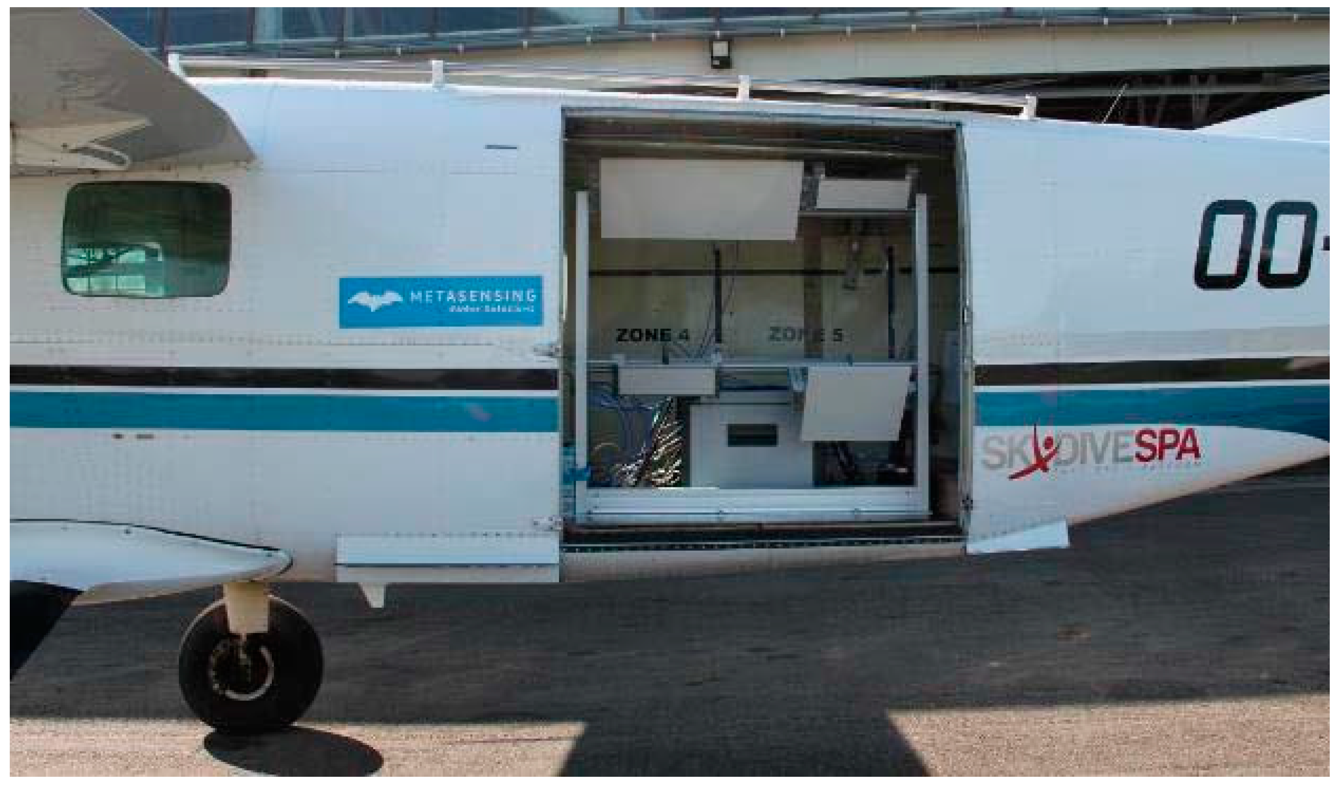
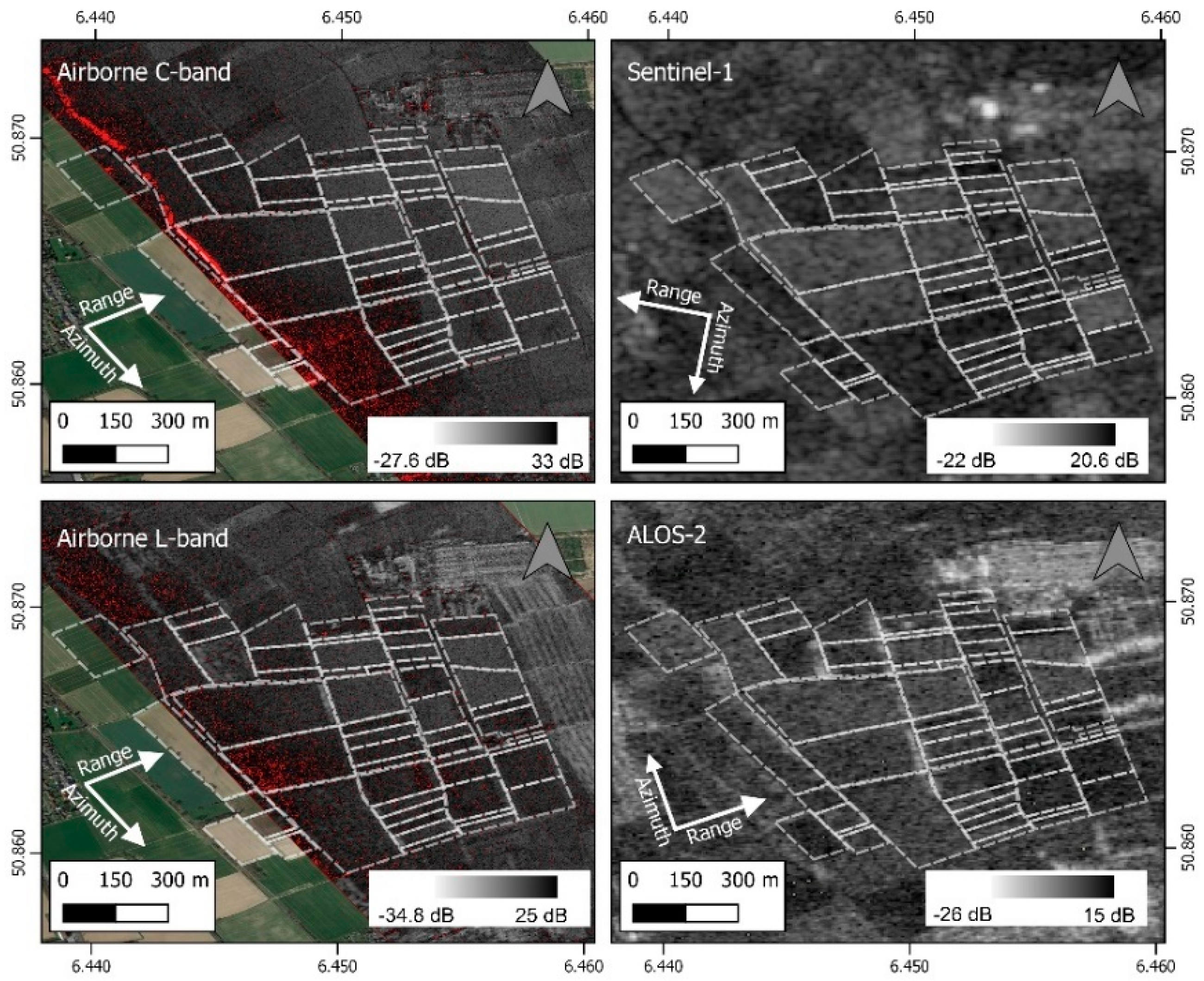
3.1. C- and L-Band Airborne SAR

The C- and L-band SAR data were acquired and processed by the company MetaSensing. The carrier was a Cessna 208 with left side-looking antennas having a nominal look angle of 45°, resulting in incidence angles ranging from 30° to 55°. The flight altitude was around 1620 m (Figure 3). To cover the larger Selhausen agricultural area, three tracks were flown per campaign day, with two ascending (track A and B) and one descending (track C) flight track and about 20% overlap among adjacent scenes. The producer-side processing steps of the radar data consist of range compression, global back-projection, geometric and radiometric calibration. Three (75 cm) corner reflectors were set up for calibration, but due to misalignment, they were only used for geometric calibration. For radiometric calibration, the C- and L-band images were calibrated among themselves, based on the estimated noise level of each data take. The first acquisition was taken as a reference value for both C- and L-band frequencies and from these, a relative noise level was calculated for each track to zero-out any temporal fluctuation. To minimize the mean offset between C-band airborne and space-borne datasets, the Sentinel-1 scene 20190620T055005a was used to calculate a global calibration factor for matching the reflectivity histograms of both data sets for a common patch over a uniformly forested area. Based on empirical values found in the literature, the L-band airborne data was calibrated using a similar procedure. After aggregating the L-band data for all missions, the backscatter histogram over the same uniformly forested area was calculated. Then, a calibration constant for the airborne L-band system was estimated such that its histogram mean would fall 2.5 dB below that of the airborne C-band radar [50]. As no polarimetric calibration was performed on the SAR data, only the backscatter coefficients of the four polarimetric channels (VV, VH, HV, and HH) are available. In this regard, the data is not suitable for eigen- and model-based polarimetric decomposition methods without further processing. The data is provided as Single Look Complex (SLC) σ⁰ in NetCDF file format.

The quad-pol (VV, VH, HV, and HH) C-band SAR sensor, used microstrip radio frequency (RF) antennas at a center frequency of 5400 MHz and transmitting a bandwidth of 200 MHz, a pulse repetition frequency of 1.89 KHz. The data were sampled at 50 MHz (

Table 2. Description of the SARSense C- and L-band radar system.

Parameter	C-Band	L-Band
Antenna Geometry (cm)	32 × 13	33 × 33, 33 × 66
Altitude (m)	1620
Velocity (Kn)	~130
Nominal look angle (°)	45
Mode	Frequency Modulated Continuous Wave-Full-Polar
Peak Power (W)	3–10
Actual PRF (kHz)	1.89
Sampling frequency (MHz)	50
Center frequency (MHz)	5400	1400/1300
Transmitted bandwidth (MHz)	200	50
Azimuth bandwidth (MHz)	100
Beamwidth (Azim. × Elev.) (°)	10 × 35	40 × 40, 20 × 40
Ground range resolution (m)	0.9–1.3	3.6–5.2
Range pixel spacing (m)	1
Azimuth pixel spacing (m)	1
Incidence angle range (°)	35–55

). The global geolocation accuracy in cross-range is 3.06 m and in slant-range 2.92 m based on average displacement as opposed to corner reflectors. The mean Noise Equivalent Sigma Zero (NESZ) was calculated over a body of standing water body in the north of every scene and is −27.6 dB. The quad-pol L-band SAR sensor also used microstrip RF antennas and the same transmission parameters as the C-band. However, the transmission bandwidth was limited by the German authorities (Bundesnetzagentur) to 50 MHz. For the dates 19, 21, 25, and 27 of June, the center frequency was 1400 MHz, whereas for the 8 and 9 of August, the center frequency was 1300 MHz. The global geolocation accuracy in cross-range is 3.05 m and in slant-range 3.01 m based on the average displacement of corner reflectors. The mean NESZ is −34.8 dB and was computed on the same water body as the C-band.

3.2. Sentinel-1 C-Band SAR

The satellites Sentinel-1 A and Sentinel-1 B are imaging the Earth with a C-band SAR instrument using a center frequency of 5400 MHz. Sharing the same orbital plane, the two satellites have a combined exact revisit time of six days, being able to map the Earth´s surface independently from weather conditions and during both day and night time [51,52]. For the period from June 2019 to August 2019 a total of 58 Sentinel-1A/B dual-polarized (VV + VH) scenes in ascending and descending mode in Interferometric Wide-Swath Mode (IW) and Ground Range Detected High Resolution (GRDH) format [53] were acquired. To obtain the highest possible number of scenes, four different orbits were used, resulting in alternating incidence angles (Desc.: 43.1°, Asc.: 30.1°, Desc.: 34.6°, Asc.: 40.1°). The IW Mode captures three-sub-swaths, combining it into a 250 km swath with a spatial resolution of 5 m by 20 m by using Terrain Observation with Progressive Scans SAR (TOPSAR). For GRDH, the resolution is resampled into a 10 m by 10 m pixel spacing. The data was obtained using the Google Earth Engine (GEE) web platform, already being pre-processed by the Sentinel-1 Toolbox SNAP [54]. The pre-processing steps consist of thermal noise removal, radiometric calibration, terrain correction using Shuttle Radar Topography Mission (SRTM) Version 3.0 Global 1 arc second dataset (SRTMGL1) and converting backscatter values to decibels (dB) using log scaling [55]. Additionally, speckle filtering was performed using a focal median filter with a kernel size of 3 by 3 pixels.

3.3. ALOS-2 L-Band SAR

Six dual-polarized (HH + HV) scenes of ALOS-2 in Stripmap Fine Mode (SM3) with a range resolution of 9.1 m and azimuth resolution of 5.3 m for the period from June 2019 to August 2019 were selected, with a revisit time of two to seven days. The scenes were recorded from two ascending and one descending orbit with an incidence angle of 34° and 35° (ascending) as well as 37° (descending) at the Selhausen test site. The Phased Array type L-band Synthetic Aperture Radar (PALSAR-2) sensor, operating with a center frequency of 1257.5 MHz and in Stripmap Fine Mode data is captured at 28 MHz bandwidth with a swath width of 70 km. The SLC data, at processing level 1.1, was provided by the Japan Aerospace Exploration Agency (JAXA) in cooperation with ESA. For further analysis, the data was radiometrically calibrated, resampled to ground range resolution of 10 m by 10 m, speckle filtered (3 by 3 pixels) using a focal median filter and geolocated using the ESA toolbox SNAP. A visual comparison between the C- and L-band air- and space borne data are displayed in Figure 4.

3.4. UASs

In the SARSense campaign, multiple UAS flights were performed, covering an area of 0.85 km². RGB images were captured by a Mavic Pro UAS as well as 5-channel multispectral and thermal infrared measurements were taken by respectively a Micasense RedEdge-M and a FLIR VUE Pro R 640 sensor mounted on a DJI M600 UAS (Figure 5). The images were georeferenced using AeroPoints GPS ground control devices [56]. The individual flight plans were created using DJI GroundStation Pro.

The Mavic Pro UAS carries a 12.7 megapixels RGB camera with an optical distortion of less than 1.5% on a 3-axis gimbal [57]. During the image acquisition, the drone had an average flight speed of 40 km/h, covering the whole test site with a flight altitude of 120 m, resulting in a spatial resolution <4 cm. Using AgiSoft MetaShape, orthomosaics for the whole Selhausen test site were created from a total of 580 nadir images, with a front overlap of 80% and side overlap of 60%. In total, five RGB orthomosaics were created, documenting the Selhausen test site over the whole SARSense campaign period. During the standard procedure to generate orthomosaics, a Digital Elevation Model (DEM) was generated from RGB data by a structure-from-motion procedure. Characteristic features were identified in multiple images and by this photogrammetric multi-view approach the 3D position and orientation of each feature is retrieved. The resulting 3D point cloud can then be converted into a DEM, which is provided here with a spatial resolution of <8 cm.

The DJI M600 was flown at an altitude of 120 m at 31 km/h with both sensors (multispectral and thermal infrared) taking nadir images every second, with the GPS position data being stored in every individual image. The FLIR VUE Pro R 640 is a radiometric thermal infrared camera with a spectral range between 7.5 to 13.5 µm, an accuracy of (±) 5 °C as well as a thermal sensitivity of 0.05 °C [58]. Equipped with a 13 mm lens, the camera has a 45° by 37° field of view with a sensor resolution of 640 by 512 pixels. The images were combined into an orthomosaic with Pix4D resulting in a spatial resolution of <40 cm.

The Micasense RedEdge-M is a 5-channel multispectral sensor, also containing a red edge and near infrared (NIR) bands besides the RGB bands. The spectral range of the individual bands can be found in

Table 3. Spectral band information for the Micasense RedEdge-M.

Band Name	Center Wavelength (nm)	Bandwidth (nm)
Blue	475	20
Green	560	20
Red	668	10
Red Edge	717	10
NIR	840	40

. Furthermore, it is equipped with a downwelling light sensor, measuring the ambient light for each band to correct lighting changes during the flight, e.g., due to changing cloud cover. The sensor was calibrated before and after every flight using the standard calibration panel. The data was combined to an 11 cm resolution orthomosaic for each date with AgiSoft Metashape.

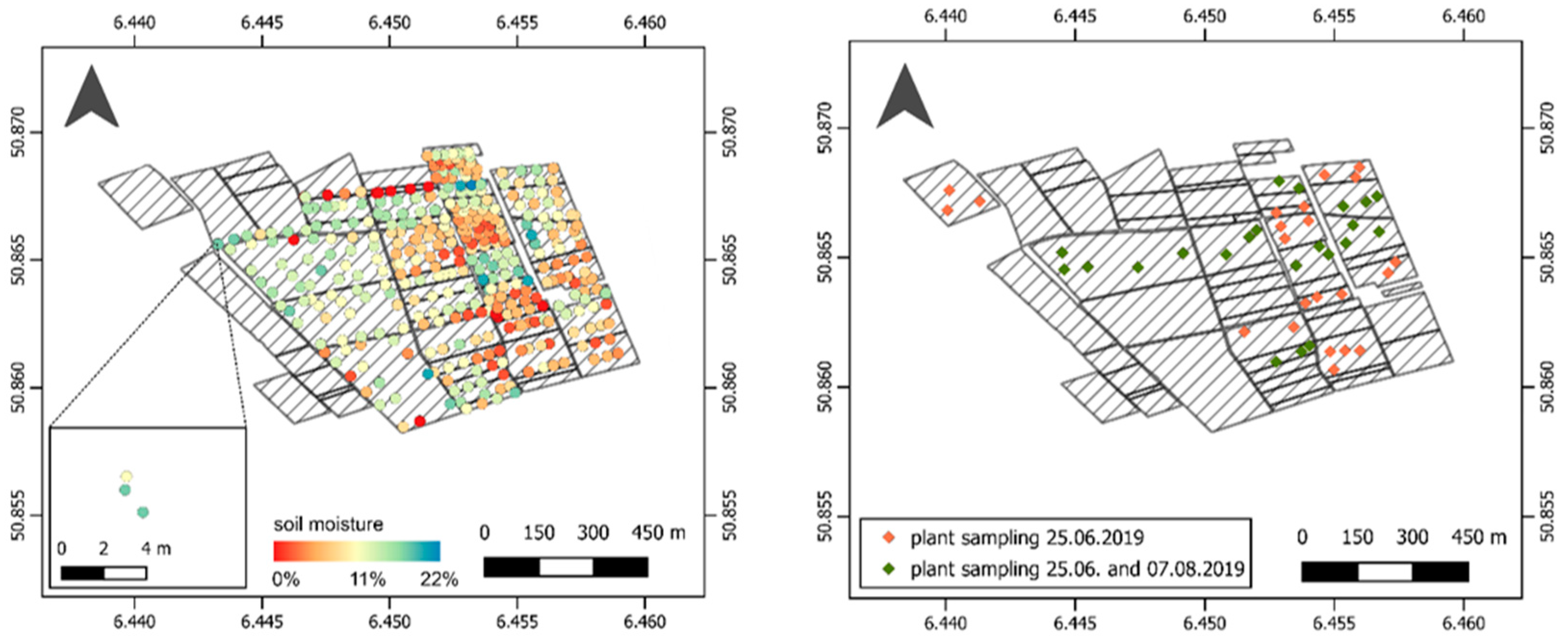
3.5. In Situ Measurements

For the duration of the SARSense flight campaign, a large number of climate, soil, and vegetation parameters were measured, both from already installed operational stations and planned field sampling. Due to the complex soil texture and the presence of different crop types, a high number of in situ soil moisture measurements and plant samplings were conducted, simultaneously or close to the SAR recordings. At the same time, permanently installed measuring stations with a high temporal resolution provided continuose data for the entire period of the SARSense campaign (from June to August 2019) at selected locations. Thanks to the combination of these two datasets, both the temporal and spatial variability of meteorological, soil, and plant parameters could be captured satisfactorily.

3.5.1. Soil Moisture

For the soil moisture measurements, a Hydra Probe II was used. It is a coaxial impedance dielectric sensor, measuring both components of the complex dielectric permittivity, allowing simultaneously measuring soil moisture and soil electrical conductivity (EC) [59]. The sensing volume is 5.7 cm by 3.0 cm, where 5.7 cm is the integrated soil moisture sensing depth. The accuracy for soil moisture is ±3%, for EC ± 0.005 S/m and for soil temperature ± 0.1 °C. As demonstrated in previous research, the Hydra Probe measurements are precise and accurate in fluids with known dielectric properties and highly correlated with soil moisture, indicating the potential of the instrument for quantitative measurement [60]. The mobile soil moisture measurements were performed using the Mobile Hydra Set, which is equipped with an internal GPS device and smartphone connection. The measured variables at the fields are sampling time, coordinates, soil temperature, soil moisture, bulk EC raw, bulk EC TC (thermal correction), pore water EC, and real and imaginary part of the dielectric permittivity (raw and TC). In total, more than 5000 measurements were collected with four Mobile Hydra Probe II during the airborne SAR acquisition dates for the whole Selhausen area (Figure 6). In addition to the soil parameters, the plant height was sampled and logged at these locations as well.

For the 27 June and 8 August, a cosmic-ray neutron sensing rover was used for measuring soil moisture. With the mobile sensor, a large spatial area can be covered within a short time, whereby the individual measurements represent an area of ~8 to 18 hectare [61] and do not represent a temporal course. As the measurement uncertainty of soil moisture depends on the number of measured neutrons, highly sensitive devices are needed [62]. Therefore, the Forschungszentrum Jülich (FZJ) cosmic rover uses an array of 9 detector units, each holding four ¹⁰BF₃-filled tubes, summing up to a total of 36 cosmic-ray neutron probes. The presented data relies on five detector units that were measuring epithermal neutrons at the time, three of which were mounted vertically in the car, whereas two were mounted horizontally. The recording interval was set to 10 seconds. [63]. The measurement of soil moisture with cosmic-ray neutron sensing relies on the inverse dependence of above-ground epithermal neutrons (energy range from ~0.2 eV to 100 keV) on the environmental water content in a footprint of 130 m to 240 m radius and 15 cm to 83 cm penetration depth [61]. The measured neutron counts were converted to soil moisture using the approach developed by Desilets et al. [64], which requires the calibration of the measured epithermal neutron intensity to soil moisture within the footprint. This was done during earlier experiments using the measurement from four other cosmic-ray neutron probes stationed in the Rur catchment [35].

In addition, a permanent SoilNet wireless sensor network consisting of five profiles (depths of −0.01, −0.05, −0.1, −0.2, −0.5, and −1 m) is operated in field F11 to measure in situ soil moisture and temperature with SMT100 sensors (Trübner Precision Instruments) [35]. The SMT100 sensor measures the transit time of an electromagnetic pulse in a 30 mm wide and 120 mm long transmission line to determine soil moisture. Due to sensor specific calibration the accuracy is for soil moisture is 1–2 Vol.% and for soil temperature ± 0.2 °C [65]. Due to the dry conditions, field F11 was irrigated multiple times by the farmer during the SARSense campaign period, with an irrigation also taking place on 27 June during an airborne SAR recording. Furthermore, 18 lysimeters (UMS GmbH) are installed on field F10, near real-time measuring the soil matrix potential, soil temperature, soil heat flux and soil water content in soil depths of 0.1 m, 0.3 m, and 0.5 m. The data from the fixed installed TERENO measuring stations are publicly available and can be found at https://www.tereno.net/ddp.

3.5.2. Plant Sampling

On the 25 of June, a total of 45 plant samples were taken for potato (F11), sugar beet (F04, F01, F47), wheat (F05, F22b, F08), barley (F33, F48b), rapeseed (F53), rye (F27, F49) and corn (F03, F24b, F06). On the 7 August, a total of 22 samples were taken for potato (F11), sugar beet (F04, F01, F47) and corn (F03, F24b, F06), where the other crops were already harvested. Within a 40 cm by 40 cm square, whole plants were harvested at each location and a representative plant was selected and sealed within a plastic bag for later laboratory measures. Furthermore, for the determination of the Chlorophyll and Carotenoid content, fresh green leaves were sampled. Using a leaf tissue puncher, five to ten leaf disks with a diameter of 9 mm were randomly punched out of the upper green leaves of a plant, each weighting between 10 mg and 20 mg. The leaf disks were transferred into 2 mL microcentrifuge tubes, immediately frozen in liquid nitrogen and transported to the FZJ. On the field site, the mean plant height (five plants at each location), the development stage of the plants according to the German Federal Biological Research Centre for Agriculture and Forestry, Federal Plant Variety Office and Chemical Industry (BBCH), LAI and chlorophyll content were measured. The LAI was determined using a SunScan plant canopy analyzer, which measures the photosynthetically active radiation (PAR) in vegetation canopies with a 1 m probe, compared to the reference PAR measured by a BF5 reference PAR sunlight sensor [66]. The chlorophyll content was measured by a SPAD-502Plus Chlorophyll meter, calculating the mean of ten measurements at each location [67].

Within three days from the field sampling, the sealed plant samples were processed in the laboratory, determining the LAI, fresh total biomass, dry weight, and canopy water content for leaves and stems separately. Here, the fresh weight of each plant is determined, and the LAI is calculated consecutively using a Li-3200 Area Meter (LiCor, Lincoln, NE, USA). After leaving the plants in a drying oven at 65 °C for five to six days, the dry weight was measured, and the canopy water content was determined by subtracting dry weight from the fresh weight.

4. Methods

In order to provide recommendations for the ROSE-L satellite mission, the potential of L-band SAR data for soil surface and vegetation parameter retrieval and its synergy effects through potential combination with C-band SAR data from existing missions like Sentinel-1 need to be evaluated. Special focus lies on the use of L- and C-band SAR data for soil moisture retrieval at high resolution as well as the added value of L-band SAR in addressing current EO measurement gaps (soil moisture, vegetation biomass, etc.) and enhanced continuity together with other missions such as Sentinel-1. The first step is to compare the airborne data with the corresponding satellite data for each flight track to assess their temporal consistency and to estimate the influence of the makeshift calibration (see Section 3.1). In the next step, the sensitivity of L- and C- band to in situ measured changes of soil moisture, plant height, vegetation water content (VWC) as well as UAS-based Normalized Difference RedEdge index (NDRE) for potato, sugar beet, wheat, and barley fields within the Selhausen test site is analyzed.

4.1. In Situ Pre-Processing

In the first step, the in situ data was filtered, using the reliability flag (Data_reliability = 0) as well as soil moisture values with 0.0 vol.% were masked as Not a Number (NaN) and not considered in further analysis. The in situ soil moisture data was collected as up to three individual measurements close to each other (within 1 m²) for each measuring location. Therefore, measurements at related points were averaged, and a new point was defined, located in the center of these points. To extract the polarimetric SAR data at these locations, the points were buffered to a circle with an 11 m radius.

4.2. Sigma Nought

The airborne backscattering intensity ${\sigma }^0$ was calculated from the SLC data by:

$${\sigma }^0=20\times {log}_{10}\sqrt{i^2+j^2}$$

(1)

with i = real part and j = imaginary part of the SLC image, following the technical specifications of MetaSensing. In the next step, a Lee filter [68] was applied with a window size of ten pixels to reduce speckle noise (Figure 7). The pixel grids were geolocated using the additional latitude and longitude information within the SLC NetCDF file.

4.3. Linear Correlation

To investigate the sensitivity of C- and L-band to changes in soil and plant parameters, the backscattering signals were correlated to the in situ measured soil moisture, VWC and plant height. Furthermore, they were compared to UAS-based NDRE, using the Near-Infrared and Red-Edge bands. To compare them with each other, a linear regression analysis was performed, where both the coefficient of determination (R²) and the Root Mean Square Deviation (RMSD) are computed for a linear regression of the two variables for each crop and band. Here, R² gives the proportion of variance of the dependent variable (backscattering signal), which can be explained by the linear model with the independent variable (surface parameter).

5. Results and Discussion

To provide a first overview of this data set, both the temporal and spatial backscattering behavior of C- and L-band from airborne and space-borne sensors are analyzed. To evaluate the potential and significance of the flight data, the respective tracks were compared with the corresponding satellite data. Moreover, we focused on soil moisture, vegetation height, and VWC, thus addressing the main objectives of the SARSense campaign. As previous studies have shown, the C- and L-band backscatter coefficients differ in their sensitivity to changes of these parameters, being majorly influenced by the crop type [10,69]. In this regard, two broad-leaved root crops (potato and sugar beet) and two narrow-leaved cereals (wheat and barley), were selected for the analysis.

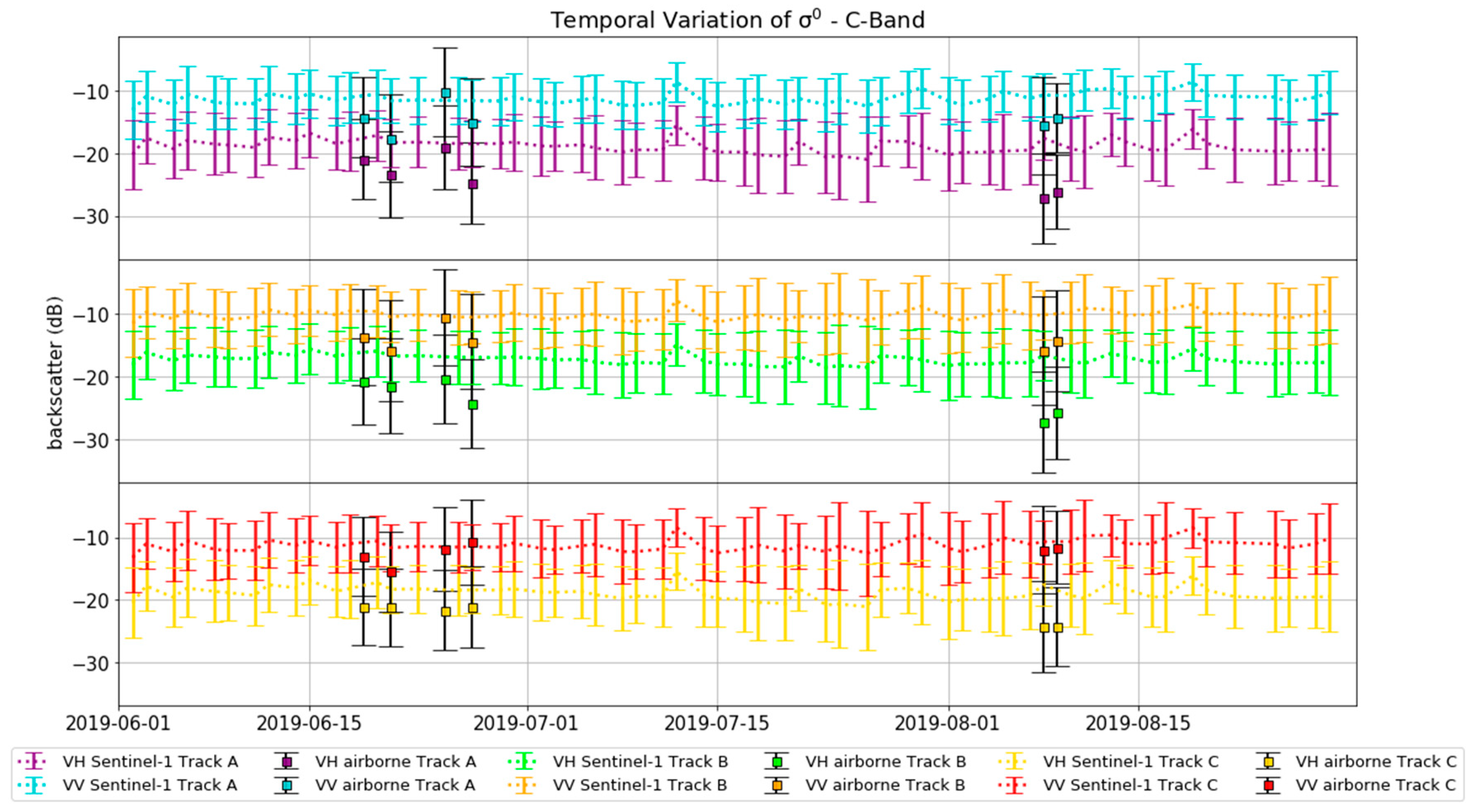
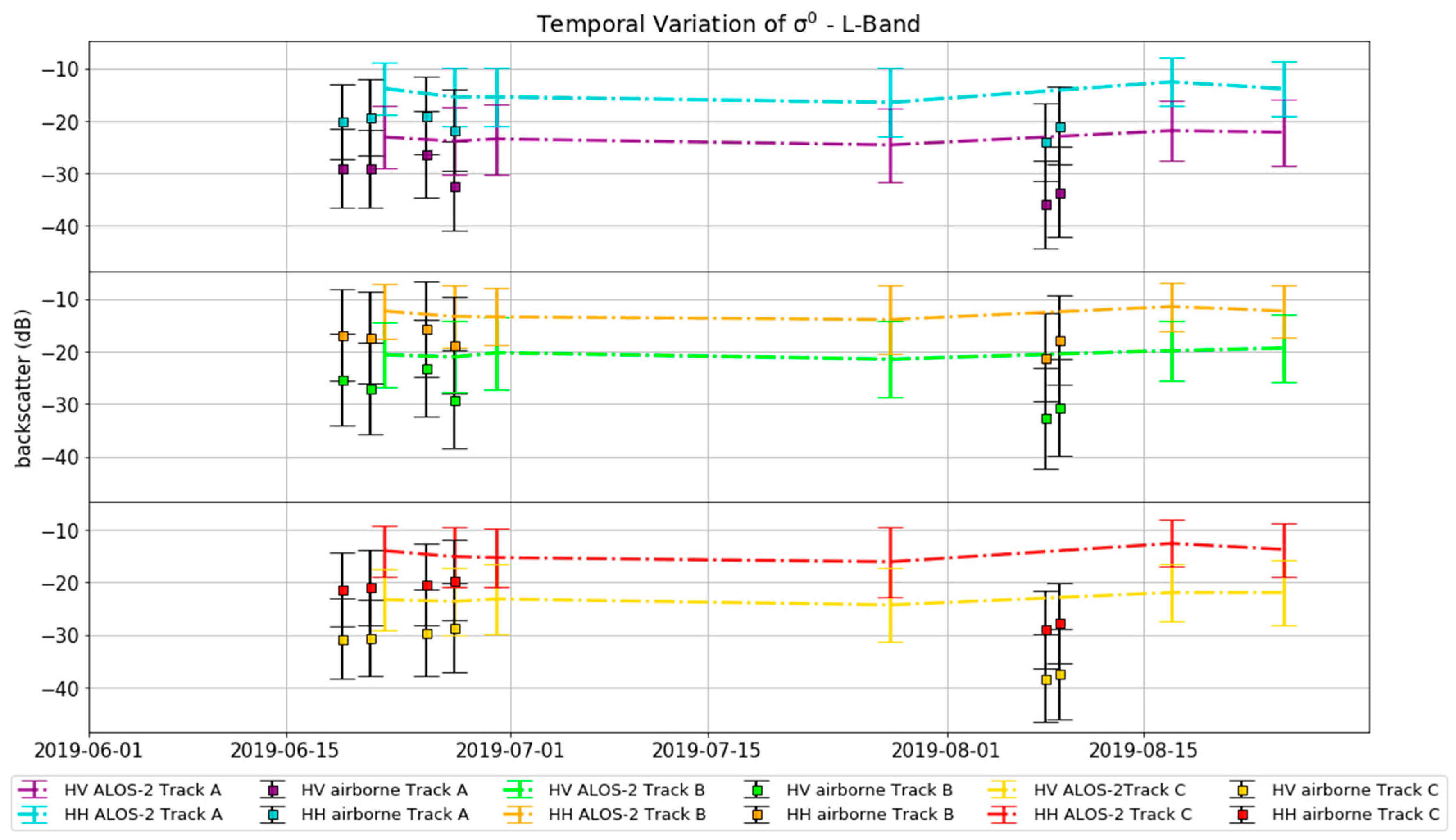
5.1. Temporal Trends of Backscattering Signals from Air- and Space-Borne SAR Data

To evaluate the quality and consistency of the airborne data, the temporal variation of each flight track is compared to the satellite backscattering signal. For the period from the 1 June to 31 August 2019, the scene-based mean and variance are calculated for both the airborne SAR data and the Sentinel-1 and ALOS-2 data of the corresponding area. By using the area-wide mean, reducing the influences of changes in individual vegetation development of different land cover types (e.g., forest and agricultural land), the effect of the airborne calibration on backscatter values can be analyzed. Since the satellite data is dual-polarized, for C-band VV and VH polarization (Figure 8), for L-band HH and HV polarization is used (Figure 9).

Concerning the C-band, the mean values of the flight tracks are in general lower than the mean values derived from Sentinel-1. Track A is about −3.23 dB in VV polarization and −5.55 dB in VH polarization, track B −3.88 dB and −6.69 dB, and track C −2.21 dB and −4.24 dB below the satellite data. Comparing the months June and August, smaller deviations can generally be observed in June, with a mean difference of −2.91 dB and −3.38 dB in VV polarization for the tracks A and B and −10.66 dB, −11.50 dB, and −9.90 dB in VH polarization for the tracks A, B, and C, respectively. Only the VV polarization signal of track C, the mean deviation is smallest in August, with −1.1 dB. In August, the larger deviation between airborne and satellite data can be observed for track A and B, with −4.19 dB and −4.94 dB in VV and −16.00 dB and −16.37 dB in VH polarization, respectively, as well as in track C with −13.59 dB in VH polarization. Here, only C band VV polarization has higher deviations in June with −1.43 dB. Looking more closely at the temporal behavior of the mean backscattering signals, the variability within the airborne data is higher than within the satellite data. In the period of the airborne SAR recordings in June and August, the mean VV polarized backscattering signals of the airborne tracks have a range of 7.36 dB (track A), 5.31 dB (track B) and 4.70 dB (track C), whereas the mean VV polarized backscattering signals derived from Sentinel-1 have a range of 1.06 dB, 0.90 dB, and 1.06 dB within the corresponding areas. For VH polarization, the mean airborne backscattering signals has a range of 8.12 dB (track A), 6.88 dB (track B), and 3.22 dB (track C), compared to the mean backscattering signals from Sentinel-1, with 1.35 dB, 1.00 dB, and 1.25 dB, respectively. In addition, the higher variability of the airborne data, also the temporal behavior differs considerably from the Sentinel-1 data. This is especially evident in June, when the airborne backscattering signals increase and decrease significantly and partially behave opposite to the Sentinel-1 backscattering signals.

The L-band backscattering signals from airborne and ALOS-2 data have the same trends as the C-band data discussed before. In general, the HH polarized airborne backscattering signals are 5.51 dB (track A), 4.66 dB (track B), and 8.01 dB (track C) below, the HV polarized backscattering signals are 7.29 dB (track A), 7.12 dB (track B), and 8.93 dB (track C) below the ALOS-2 backscattering signals within the observation period. Here the deviation between the two data sets becomes particularly clear in track C in August, where the gap between the mean backscattering signals is the largest. In this regard, the change in frequency from 1400 MHz in June to 1300 MHz in August needs to be considered as one cause for this behavior, even though this trend is not as prominent in the other tracks. Focusing on the temporal variability of airborne and ALOS-2 backscattering signals in June, where both data sets have the most comparable temporal frequency, the airborne HH polarized backscattering signals have a range of 2.81 dB (track A), 3.06 dB (track B), and 1.75 dB (track C), compared to 1.61 dB, 1.08 dB, and 1.30 dB from ALOS-2 images, respectively. For HV polarization, the airborne backscattering signals have a range of 5.93 dB (track A), 5.95 dB (track B), and 2.08 dB (track C) compared to 0.78 dB, 0.80 dB and 0.46 dB from ALOS-2 scenes, respectively. Like the airborne C-band data, also the airborne L-band data has higher variability as well as a stronger de- and increases of the backscattering signal can be found in the airborne data. The temporal behavior of the airborne backscattering signal is similar to the one observed in the airborne C-band data, while the ALOS-2 data does not change to an equal extent.

As shown in the temporal analysis of the C- and L-band data, the airborne data differ from the space-borne data both in absolute values and in their temporal behavior. While the satellite-based data show only slight changes in the observed period between individual images, the corresponding airborne data exhibit a very strong change, which is also partly opposite to the space-borne data. This becomes particularly evident in June, when the greatest variability between the scene-based mean values within the airborne data in both C- and L-band is observed, which is not reflected in the backscatter values of the satellite data. The strong variability of the backscattering signals is therefore rather caused by the sub-optimal calibration than by changes in soil and plant parameters. Without further processing, a comparison between absolute airborne backscattering signals and surface parameters over multiple dates would lead to biased results. In this regard, we focus on the time series of Sentinel-1 and ALOS-2 data when comparing backscattering signals between C- and L-band to changes in surface parameters using in situ measurements from different dates. The airborne data is used for scene-based (spatial) analysis. In conclusion to the preceding analysis, the main results are the following:

• Due to sub-optimal radiometric calibration, both C- and L-band airborne data differ in absolute values and in their temporal behavior from corresponding space borne data.
• The use of airborne SAR data from different acquisition dates for analyzing the temporal behavior of surface parameters would lead to biased results.

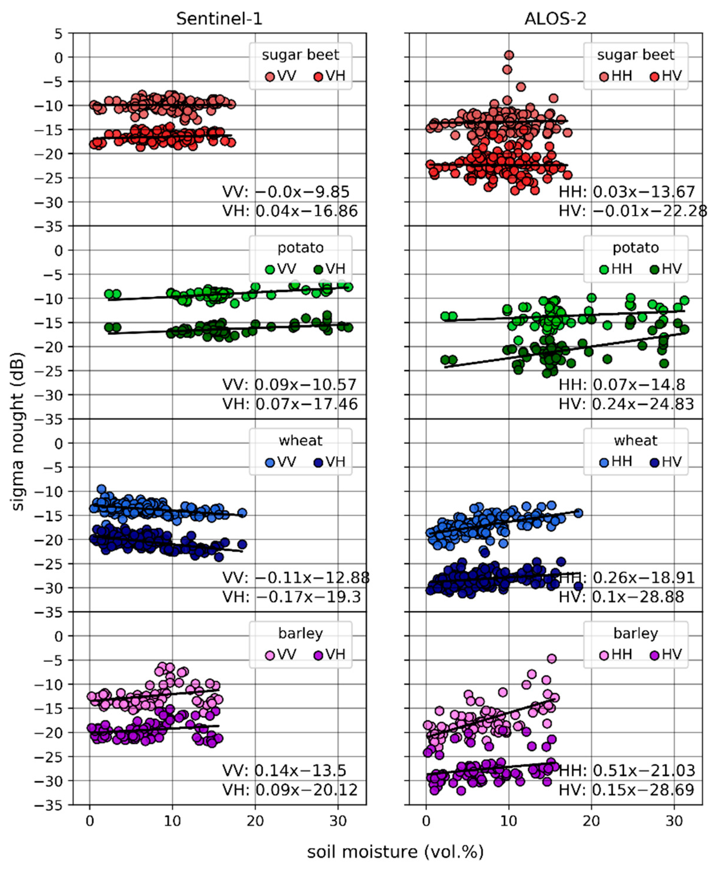
5.2. Backscattering Signal and Soil Moisture

To evaluate the behavior of the backscattering signal with respect to changes in soil moisture, the area-weighted means from backscattering signals in a radius of 11 m around the respective measurement location were correlated with the respective soil moisture values. In this regard, the Sentinel-1 scenes from the 21 and 27 June were correlated with the soil moisture values measured on the corresponding days, both scenes recorded in descending mode with an incidence angle of 43° over the Selhausen test site. ALOS-2 scenes from the 22 and 27 June were correlated with the in situ measurements of the 21 and 27 June, with incidence angles of 34° and 35°, both in ascending mode. As the field F11 was irrigated on the 27 June by the local farmer, the highest soil moisture values can be observed on the potato fields with 2 vol.% to 31 vol.%, whereas the other fields have soil moisture values ranging between 1 vol.% and 17 vol.%. development stage of sugar beet in June is between BBCH 35 and 40, for potato 31, for wheat 77 and for barley between 77 and 92.

With R² between 0.00 and 0.42 no or only moderate correlations between backscattering signals and soil moisture are present. At L-band, the highest correlation can be observed in the co-polarized channel for the barley fields, with R² = 0.42, while the lowest correlation is observed for the sugar beet fields with R² = 0.00 in both co- and cross-polarized channels (Figure 10;

Table 4. The coefficient of determination (R²) and Root Mean Square Deviation (RMSD) of the linear regression between backscattering signal and soil moisture.

Crop.		C-Band VV	C-Band VH	L-Band HH	L-Band HV
Sugar Beet	R2	0.00	0.03	0.00	0.00
	RMSD	1.15	0.67	6.05	5.25
Potato	R2	0.35	0.20	0.05	0.32
	RMSD	0.54	0.64	3.56	4.57
Wheat	R2	0.18	0.28	0.31	0.07
	RMSD	0.95	1.16	2.28	2.07
Barley	R2	0.09	0.05	0.42	0.06
	RMSD	4.22	3.02	6.86	7.23

). In C-band, the maximum correlation can be observed in the co-polarized channel for the potato fields with R² = 0.35, whereas the co-polarized channel for the sugar beet fields is uncorrelated with R² = 0.00. It should be noted here that the data for the potato fields refer to only two individual fields and thus a smaller number of SAR signals are correlated with the soil moisture data, which at the same time show the highest variability. In this sense, the observed correlation is less significant compared to the other studied fields. Moreover, the directional scattering caused by the periodic tillage structure of potato fields can lead to an increase of the backscattering signal up to 3 dB, depending on the row direction, influencing the comparability of the backscattering signals for the two observed potato fields [70]. While most correlations are positive, the C-band backscattering signal in wheat correlates negatively with soil moisture in both channels. Here, the cross-polarized channel with R² = 0.28 reaches the second highest value at C-band, while the co-polarized signal correlates with R² = 0.18. Looking at the plant height at the in situ measuring soil moisture sites, most of the wheat plants range between 60 cm to 100 cm. Correlating the backscattering signal to these plant heights, no significant negative correlation can be observed, with R² = 0.07 in co- and R² = 0.04 in the cross-polarized channel. In this regard, different plant heights related to soil moisture are not likely causing this behavior. A decreasing trend of backscattering signal in elongated, narrow-leaved plants like wheat and barley, caused by high absorption rates of densely arranged thin plant stems, is previously observed with increasing biomass or VWC in X-, C-, and L-band [71,72,73]. In this respect, increasing soil moisture could be accompanied by increasing water content of the vegetation, leading to an attenuation of the soil scattering component and thus to an absolute reduction of the backscattering signal. Increasing backscattering signals from drying soil at very low soil moisture conditions due to increasing subsoil reflectance, as observed by Morrison et al. [74], is not yet described for soils with vegetation cover.

Considering the RMSD, L-band tends to have significantly higher variance within the backscattering signal than C-band, with a mean RMSD of 5.75 dB compared to 1.54 dB. Here, larger RMSD are observed in the co-polarized channels, with a mean difference to the cross-polarized channels of 0.41 dB at L-band and 0.34 dB at C-band. The greatest difference in RMSD between C- and L-band can be observed in sugar beet fields. Here the L-band backscattering signals are much more scattered and appear randomly distributed around a fixed level. Due to the deeper penetration into the vegetation cover and soil layer, the L-band contains information not only from surface backscattering, but also from backscattering of the fleshy taproots, which are shallowly buried in the soil and have a high water content of up to 80% [75]. This likely causes a worse correlation between L-band backscattering and soil moisture compared to other crops.

Looking at the correlations of both polarizations, it can be observed that in L-band always one polarization shows a significantly higher correlation, except for sugar beet. In this regard, the co-polarized signal from the narrow-leaved crops wheat and barley has significantly higher R² values (0.31 and 0.42) than the cross-polarized signal (0.07 and 0.06), as observed in previous studies [76]. In the potato plant with broad leaves, the trend is reversed, with R² = 0.32 in the cross-polarized signal and R² = 0.05 in the co-polarized signal. Here the C-band tends not to have such large differences between cross- and co-polarization. At the potato and wheat fields, where the highest correlations are observed, they differ significantly less. For potato, R² = 0.35 in the co-polarized signal and R² = 0.20 in the cross-polarized signal, while for wheat R² = 0.18 and R² = 0.28, respectively. This trend can also be observed in the slopes of the linear regressions, where the values in the L-band between the co- and cross-polarization signals differ more than at the C-band. Excluding the sugar beet, where no correlation can be observed in both bands, the mean difference between the slopes of co- and cross-polarized channel for each crop at L-band is 0.26, whereas the difference at the C-band is only 0.04. The larger differences between the co- and cross-polarized channels at the L-band indicate that two different scattering mechanisms are measured in each polarization, whereas at the C-band in both polarizations rather only one scattering mechanism is prominent. Since the L-band waves should penetrate deeper into the vegetation layer, the co-polarized signal contains more of the surface backscattering signal, whereas the cross-polarized signal measures more volume backscattering [77]. The C-band, with a wavelength about four to five times shorter, penetrates less into the vegetation layer than L-band and, therefore, might contain only small signal contributions of soil surface scattering. In this regard, both co- and cross-polarized channels contain mainly the same information from vegetation volume scattering [10]. Summing up the results:

• C- and L-band do not show any correlation for sugar beet.
• The co-polarized L-band signal has the highest correlation to soil moisture regarding the narrow-leafed crops.
• Two different scattering mechanisms are measured with co- and cross-polarization at L-band, while only one scattering mechanism is prominent at C-band.

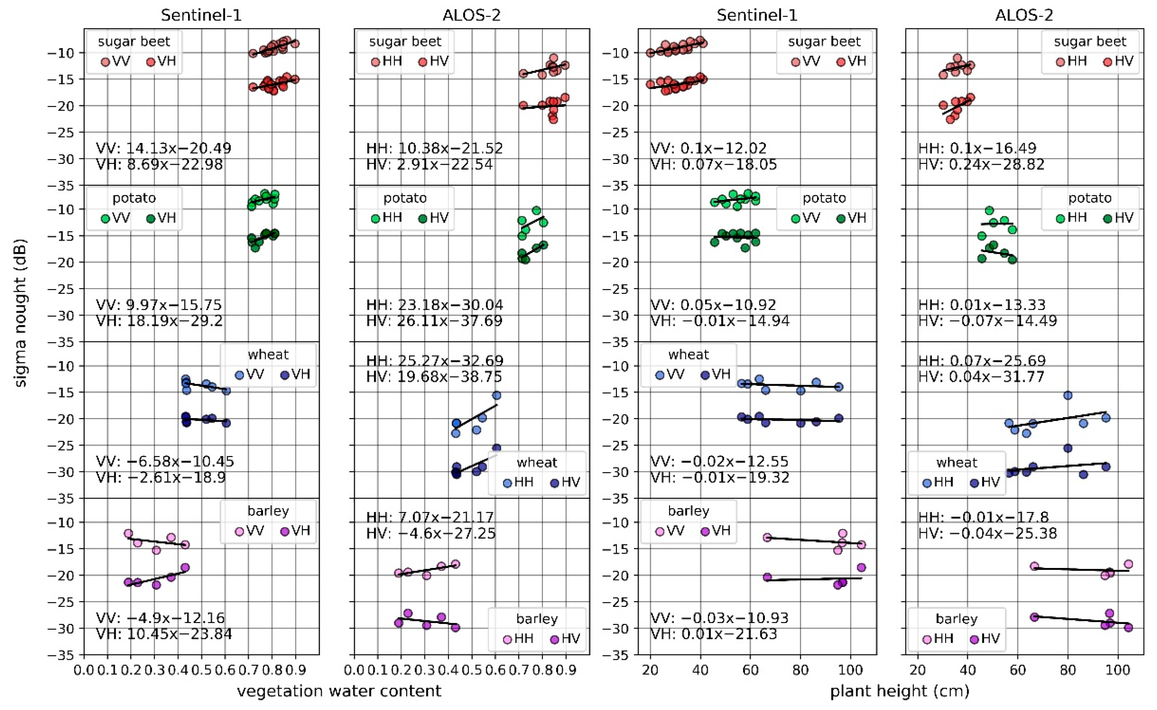
5.3. Backscattering Signal and Plant Parameters

To evaluate the behavior of C- and L-band backscattering on changes in plant parameters, the VWC and plant height measurements from the 25 June and 7 August 2019 were compared to the signals from the co- and cross-polarized channels (VV and VH for C-band, HH and HV for L-band). As the recordings only partially match the in situ measuring dates, Sentinel-1 scenes from the 26 June and the 7 August as well as the ALOS-2 scene from the 27 June were correlated. Since there is a ten-day difference between in situ measurements and ALOS-2 recordings in August, these data were not included due to temporal decorrelation. As wheat and barley were already harvested in August, information on plant parameters was only measured for sugar beet and potato fields this month. The VWC is between 72% for sugar beet, between 43% and 60% for wheat, 19% and 43% for barley, and for potato the VWC is between 71% and 81%. For plant height, sugar beet was measured between 20 cm and 40 cm for the C-band and 30 cm and 40 cm for the L-band, potatoes between 40 and 60 cm, wheat between 55 cm and 95 cm, and barley between 65 cm and 105 cm (Figure 11). To evaluate the correlation between backscattering signals and plant parameters, again linear regressions are calculated and the related R² and RMSD are compared.

Looking at the VWC, C-band tends to be more sensitive to changes in vegetation water content for sugar beet, while especially the co-polarized signal with R² = 0.64 performs better than the L-band co-polarized signal with R² = 0.27 (

Table 5. R² and RMSD of the linear regression between backscattering signal and vegetation water content (VWC).

Crop		C-Band VV	C-Band VH	L-Band HH	L-Band HV
Sugar Beet	R2	0.64	0.24	0.27	0.01
	RMSD	0.20	0.40	0.65	1.65
Potato	R2	0.24	0.55	0.27	0.76
	RMSD	0.41	0.36	1.90	0.28
Wheat	R2	0.33	0.12	0.58	0.65
	RMSD	0.37	0.21	1.95	0.90
Barley	R2	0.16	0.63	0.60	0.17
	RMSD	1.02	0.50	0.26	0.83

). For potato, L-band tends to be more sensitive, with R² = 0.24 and R² = 0.55 for co- and cross-polarized channel in C-band and R² = 0.27 and R² = 0.76 at L-band. Apart from the cross-polarized channel within the barley fields, the L-band signal is much more sensitive to changes in VWC for the elongated, narrow-leaved crops, with R² values between 0.58 and 0.65 compared to R² values between 0.12 and 0.33. In contrast to soil moisture, negative correlations can be observed for wheat at C-band as well as for barley at C- and L-band. In this regard, the trend that backscattering signals decrease with increasing VWC in elongated plants can be observed in both bands. While at C-band the trend can be observed for VWC values ranging between 20% and 40% (barley) for co-polarization as well as between 40% and 60% (wheat) for both polarizations, at L-band this behavior can be only observed for values between 20% and 40% for cross-polarization in the barley fields. Since the correlation here is made only with five to six in situ measurements (a small set of samples), further investigations need to be done to confirm this observation.

The correlation between the backscattering signal and plant height is lower compared to the VWC. For C-band, only the co-polarized signal from the sugar beet field has a significant correlation with R² = 0.55, while all other regressions have R² values ranging between 0.00 and 0.25. For L-band, the highest correlation can be observed in the cross-polarized signal from sugar beet field with R² = 0.41, while the other R² values range between 0.00 and 0.22 (

Table 6. R² and RMSD of the linear regression between backscattering signal and plant height.

Crop		C-Band VV	C-Band VH	L-Band HH	L-Band HV
Sugar Beet	R2	0.55	0.25	0.22	0.41
	RMSD	0.22	0.41	0.73	1.24
Potato	R2	0.13	0.00	0.00	0.08
	RMSD	0.47	0.80	2.61	1.09
Wheat	R2	0.08	0.11	0.22	0.10
	RMSD	0.51	0.21	3.63	2.30
Barley	R2	0.12	0.01	0.05	0.22
	RMSD	1.07	1.34	0.62	0.78

). Looking at the behavior of the respective polarizations within the bands, the co-polarized signals at C-band and the cross-polarized signals at L-band have higher R² values for the broad-leaved plants. No such trend can be observed in the narrow-leaved crops. However, it should also be pointed out that due to the low number of measurements this observation requires further analysis.

With a mean RMSD of 1.27 dB, the L-band is much more scattered around the linear regression models than the C-band with a mean RMSD of 0.52 dB. This trend can also be observed when looking only at the correlations where both C- and L-band are shifted by one day with the in situ measurement. In previous studies, the difference between C- and L-band was observed in wheat, barley, and rapeseed fields, where the L-band backscattering signal generally has higher standard deviations than the C-band, especially pronounced in the first months of the year. This difference is furthermore higher in the VV polarized backscattering signal than in the HH polarized signal [78]. Summarizing the analysis, the main results are the following:

• For both C- and L-band, higher correlation can be observed with VWC than plant height.
• The attenuation effect of cereals on the backscattering signal is most prominent at the C-band, resulting in negative correlations.

5.4. Backscattering Signal and Interception

A scene-based analysis was performed to study the airborne SAR data on the different behavior of C- and L-band cross- and co-polarized channels, comparing only data from simultaneous recordings. Flight track C was used for this purpose, as it has the smallest absolute deviation from satellite data and comparatively smaller temporal, calibration-caused variations than track A and B. During the SAR acquisition on 27 June, the potato field F11 was partially irrigated by the local farmer (Figure 12, dashed line). A direct comparison between the backscattering signal from a non-irrigated and irrigated area is possible, sharing the same surface and observation parameters. The field F11 is located at the near-range of the airborne observation, with incidence angles ranging between 32° and 43°. As the backscattering signal is depending on the incidence angle, SAR-specific range-dependencies can usually be observed with decreasing backscattering intensity related to increasing incidence angles [79,80]. As shown in Figure 12, a reverse trend is present at field F11 with increasing backscattering values related to increasing incidence angles. Here, the L-band HH polarization has an increase of 0.61 dB, the HV polarization an increase of 0.45 dB per one degree of incidence angle while the C-band HH polarization has an increase of 1.02 dB and HV polarization one of 0.86 dB.

To compare both bands and polarizations, the trend was adjusted using a linear regression model and the backscattering values were leveled to the respective measured mean. Comparing the histograms from detrended backscattering signals, the largest difference between irrigated and non-irrigated areas are observed at L-band, with a difference of 3.27 dB in the cross-polarized and 2.20 dB in the co-polarized channel between the respective mean values. This is in line with the results of Vermunt et al. [81], which measured a difference of 3 dB for cross-polarization and 2 dB for co-polarization after light precipitation events for sweet corn, related to the water stored temporally in the interception. The C-band for the potato field has a difference of 1.98 dB in the cross-polarized and 1.78 dB in the co-polarized channel, being less influenced by the interception as well as both polarizations are behaving more similar. The effects of interception water on backscattering signals for potato were also observed previously, even though the related changes were described significantly lower from X-, C-, and L-band recordings three hours after a precipitation event by Riedel et al. [82]. Here, the time between a precipitation or irrigation event and a SAR observation seems to be crucial. While Ulaby [83] stated, that the effect of precipitation is only visible for about one hour in wheat fields, at least the time in potatoes is likely to be similarly short in this regard.

The different behavior of C- and L-band might be again explained by the different penetration depth of the wavelengths. Due to the shallower penetration into the vegetation cover, C-band is sensitive to the water stored on the surface of the vegetation cover after precipitation or irrigation, while the L-band is also sensitive to the interception water stored within the vegetation. In this sense, the simultaneous recording of C- and L-band during or shortly after precipitation events or irrigation can be used to obtain different information about the interception storage of agricultural plants. In addition, the relationship between C- and L-band backscatter could be used to distinguish between backscatter changes related to changes in soil moisture or plant water content and changes related to interception shortly after or during precipitation events.

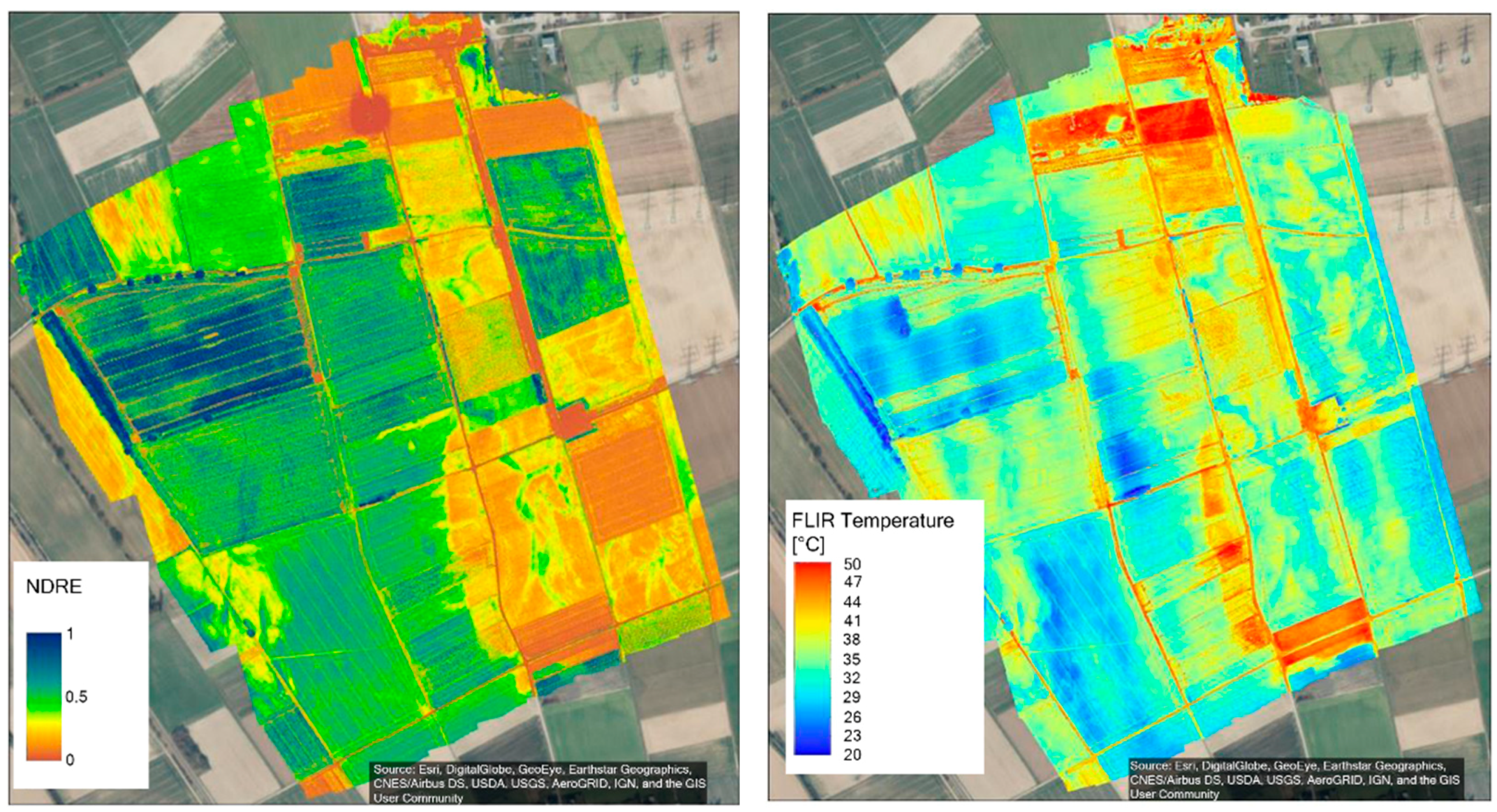
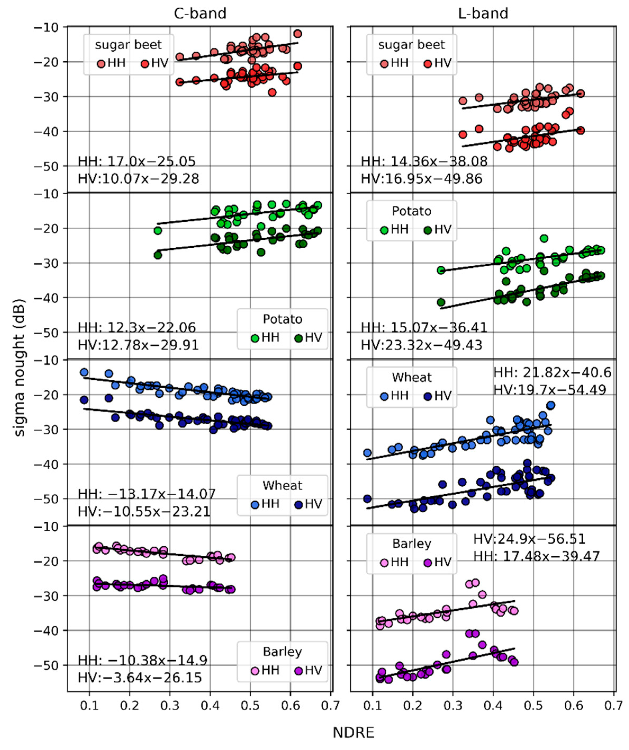
5.5. Backscattering Signal and Normalized Difference Red Edge Index

To analyze the behavior of C- and L-band backscattering signals to other remote sensing vegetation indices, it was compared to the NDRE. For the 27 June, UAS multispectral images were compared to the respective co- (HH) and cross-polarized (HV) SAR images from track C at the locations of soil moisture measurements within an 11 m radius. In the first step, both the C- and L-band images were detrended as described before. For this purpose, a uniform forest patch in the north of the scenes was selected, to calculate the underlying calibration-related range-trend and minimize the influence of the different vegetation covers at the Selhausen test site. The forest patch covers the whole range of incidence angles, spanning from the near- to far-range of the scenes. Opposite to the potato field F11, the range-trends are similar in C- and L-band here. The co-polarized C-band signal has a trend of 0.49 dB per one degree of incidence angle, the cross-polarized signal a trend of 0.47 dB. The L-band co-polarized signal has a trend of 0.46 dB, while the cross polarized signal has the smallest trend with 0.35 dB. Equal to the analysis before, the focus was on the sugar beet, potato, wheat, and barley. The NDRE values range from 0.3 to 0.6 for sugar beet, 0.25 to 0.75 for potato, 0.1 to 0.55 for wheat, and 0.1 to 0.45 for barley. In general, for the broad-leaved crops sugar beet and potato, L-band has higher correlations than C-band, while for the narrow-leafed crops C-band has higher correlations (Figure 13;

Table 7. R² and RMSD of the linear regression between backscattering signal and NDRE.

Crop		C-Band HH	C-Band HV	L-Band HH	L-Band HV
Sugar Beet	R2	0.22	0.14	0.24	0.18
	RMSD	3.75	2.24	2.37	4.70
Potato	R2	0.34	0.40	0.46	0.64
	RMSD	2.64	2.26	2.44	2.76
Wheat	R2	0.74	0.56	0.55	0.47
	RMSD	0.87	1.26	5.63	6.37
Barley	R2	0.74	0.22	0.39	0.53
	RMSD	0.42	0.54	5.45	6.38

). The highest correlation at L-band can be found in the cross-polarized channel for potato with R² = 0.64, while the highest correlation at C-band can be found in the co-polarized channel for wheat and barley with R² = 0.74. The lowest correlation can be found in the cross-polarized channel for sugar beet, with R² = 0.14 and R² = 0.18 for C- and L-band. For the L-band, this is consistent with the low correlations observed in the previous analyses in sugar beet, although the correlation of the backscattering signal with NDRE is higher than that of soil and plant parameters. For the narrow-leaved crops, the co-polarized channel has significantly higher R² values at C-band, while the difference is not as prominent at L-band. The trend of decreasing backscattering signal with increasing VWC at the C-band can also be observed with Negative correlations in the C-band, as observed in the satellite data, also exist for NDRE for the cereals. The negative correlation is found in both wheat and barley fields and in both polarizations, being generally stronger in the wheat as well as the co-polarized channel. In this respect, it the behavior agrees in large parts with the results from the satellite data.

In conclusion to the preceding analysis, the main results are

• For the broadleaf crops, L-band shows highest correlation with NDRE, while for the narrow-leafed, C-band shows highest correlation.
• C-band is highly affected by the attenuation effects of cereals, resulting in negative correlations with NDRE, while L-band is not affected.

6. Conclusions and Outlook

With SARSense, we present an extensive multi-frequency SAR time-series dataset, including both air- and space-borne C- and L-band recordings, accompanied by in situ measurements of the soil and plant parameters (e.g., soil moisture and vegetation water content) as well as high resolution multispectral and thermal data from UAS and cosmic-ray neutron sensing. The large variety of crops grown at the Selhausen test site and the high temporal and spatial resolution measurements provide a comprehensive database for SAR-based research on agricultural land, especially under low soil moisture conditions (around 8 to 17 vol.%). Here, both small-scale and temporally short correlations between backscattering signal and surface parameters (e.g., interception) as well as more general correlations (e.g., the difference between narrow and broad leaf crops) can be observed. Furthermore, a detailed analysis between C- and L-band for different crop types is possible, indicating characteristic backscattering behavior caused by the shape and habitus of the plants. By this, the SARSense campaign continues and extends previous SAR campaigns over the Selhausen test site to provide in-depth and up-to-date knowledge for ongoing and future SAR missions. The dataset as well as the related campaign report can be accessed at https://earth.esa.int/eogateway/campaigns/sarsense-technical-assistance-for-airborne-measurements-during-the-sar-sentinel-experiment (accessed 20 January 2020).

Due to misaligned corner reflectors, no absolute calibration of the airborne SAR data was possible. This is significantly influencing the comparability of the backscattering signals from individual flight tracks. The calibration of the airborne data with the Sentinel-1 scene could not adequately compensate for the error. In this sense, direct comparison between satellite data and airborne data is not possible without further actions, and inter-scene analysis of airborne data would lead to biased results. However, the response of cross- and co-polarized backscattering signals at C- and L-bands to changes in soil and plant parameters across dates can be studied in detail using satellite Sentinel-1 and ALOS-2 data. By using a scene-based approach to analyze the airborne C- and L-band data, they can be used as well for comparing the backscattering signal to the respective ground and plant parameters measured on the same day, although the scenes need to be detrended from the prevailing incidence angle dependency.

The correlations between backscattering signal and surface parameters highly vary between the investigated crops, indicating that no general statement can be made on whether C- or L-band is more sensitive to a respective status or dynamic of a soil or plant parameter. Moreover, neither cross- nor co-polarization is generally performing better in terms of sensitivity to these parameters as this sensitivity is specific for each investigated plant. Overall, during the extremely dry conditions of the campaign period, the lowest R² values are observed in the correlation of the SAR signal to soil moisture, with R² values ranging between 0.00 and 0.35 at C-band and 0.00 and 0.42 at L-band. Almost no correlation can be observed for the sugar beet, indicating that no information from surface backscattering is present for C-band while at L-band, the shallow buried sugar beets are leading to a speckle induced decorrelation. As seen in potato, where the C-band has a higher R² value than L-band in the respective polarization, the backscattering signal reflected by the canopy surface at C-band may sometimes have a stronger correlation to the soil moisture measured by the more deeply penetrating L-band. Since this is of particular interest when using multi-frequency methods for soil moisture estimation on agricultural sites, further research should be conducted to determine for which plants this occurs. For the narrow-leaved plants, wheat and barley, L-band co-polarization has the highest R² values. In terms of VWC, the L-band has higher correlations for the cereals like wheat and barley, while for the broad-leaved crops, the C-band shows a higher correlation. For the Normalized Difference Red Edge index, the trend is reversed, with higher R² at C-band for the narrow leaf plants and slightly higher R² values at L-band for the broadleaf plants. Since NDRE is also positively correlated with VWC, further research examining their interdependencies for these plant types should be conducted to understand this behavior [84]. Negative correlations at C-band can be observed for the narrow-leaved plants for all soil and plant parameters studied, clearly demonstrating the attenuation effect on the backscattering signal within the elongated plants in both vertical and horizontal polarizations also after the heading stage, as observed in previous studies [69]. This should be considered, when estimating soil and plant parameters using change-based methods at C-band, e.g., alpha-approximation method [69]. Regarding the vegetation height, the backscattering signals correlated only very weakly to changes. Only the C-band co-polarized signal for sugar beet is an exception with R² = 0.56, whereby the correlation is largely caused by the relationship between plant height and VWC.

In almost all cases, the backscattering signals of C- and L-band contain a different amount of information about the observed agricultural fields and their individual soil and plant parameters. Therefore, the simultaneous acquisition of C- and L-band SAR data will result in an additional gain in remote sensing of soil and plant. This is of particular interest for agricultural sites with different vegetation types and phenologies, where the sensitivity of the C- and L-band to soil and plant parameters differ.

References

1. Arnell, N.W.; Gosling, S.N. The impacts of climate change on river flood risk at the global scale. Clim. Chang. 2016, 134, 387–401. [Google Scholar] [CrossRef] [Green Version]
2. IPCC. Climate Change 2013: The physical Science Basis: Working Group I Contribution to the Fifth Assessment Report of the Intergovernmental Panel on Climate Change; Cambridge University Press: Cambridge, UK, 2013. [Google Scholar]
3. Dudula, J.; Randhir, T.O. Modeling the influence of climate change on watershed systems: Adaptation through targeted practices. J. Hydrol. 2016, 541, 703–713. [Google Scholar] [CrossRef] [Green Version]
4. Wu, P.; Christidis, N.; Stott, P. Anthropogenic impact on Earth’s hydrological cycle. Nat. Clim. Chang. 2013, 3, 807–810. [Google Scholar] [CrossRef]
5. UNFCCC. Adoption of the Paris Agreement; Report No. FCCC/CP/2015/L.9/Rev.1; UNFCCC: Paris, France, 2015. [Google Scholar]
6. Sheffield, J.; Wood, E.F.; Pan, M.; Beck, H.; Coccia, G.; Serrat-Capdevila, A.; Verbist, K. Satellite Remote Sensing for Water Resources Management: Potential for Supporting Sustainable Development in Data-Poor Regions. Water Resour. Res. 2018, 54, 9724–9758. [Google Scholar] [CrossRef] [Green Version]
7. Tang, Q.; Gao, H.; Lu, H.; Lettenmaier, D.P. Remote sensing: Hydrology. Prog. Phys. Geogr. Earth Environ. 2009, 33, 490–509. [Google Scholar] [CrossRef]
8. Gleason, C.J.; Wada, Y.; Wang, J. A Hybrid of Optical Remote Sensing and Hydrological Modeling Improves Water Balance Estimation. J. Adv. Model. Earth Syst. 2018, 10, 2–17. [Google Scholar] [CrossRef]
9. ESA. Copernicus L-band SAR Mission Requirements Document. Available online: https://esamultimedia.esa.int/docs/EarthObservation/Copernicus_L-band_SAR_mission_ROSE-L_MRD_v2.0_issued.pdf (accessed on 20 January 2020).
10. El Hajj, M.; Baghdadi, N.; Bazzi, H.; Zribi, M. Penetration Analysis of SAR Signals in the C and L Bands for Wheat, Maize, and Grasslands. Remote Sens. 2019, 11, 31. [Google Scholar] [CrossRef] [Green Version]
11. De Roo, R.D.; Yang, D; Ulaby, F.T.; Dobson, M.C. A semi-empirical backscattering model at L-band and C-band for a soybean canopy with soil moisture inversion. IEEE Trans. Geosci. Remote Sens. 2001, 39, 864–872. [Google Scholar] [CrossRef]
12. Steele-Dunne, S.C.; McNairn, H.; Monsivais-Huertero, A.; Judge, J.; Liu, P.-W.; Papathanassiou, K. Radar Remote Sensing of Agricultural Canopies: A Review. IEEE J. Sel. Top. Appl. Earth Obs. Remote Sens. 2017, 10, 2249–2273. [Google Scholar] [CrossRef] [Green Version]
13. NASA. Available online: https://nisar.jpl.nasa.gov/mission/quick-facts/ (accessed on 17 June 2020).
14. European Space Agency. AgriSAR 2006: Agricultural Bio-/Geophysical Retrievals from Frequent Repeat SAR and Optical Imaging; European Space Agency: Paris, France, 2006. [Google Scholar]
15. European Space Agency. TropiSAR: Tropical Forest Biomass Mapping Using L- and P-Band SAR; European Space Agency: Paris, France, 2009. [Google Scholar]
16. Chapin, E.; Chau, A.; Chen, J.; Heavey, B.; Hensley, S.; Lou, Y.; Machuzak, R.; Moghaddam, M. AirMOSS: An Airborne P-band SAR to measure root-zone soil moisture. In Proceedings of the 2012 IEEE Radar Conference, Atlanta, GA, USA, 7–11 May 2012; IEEE: Piscataway, NJ, USA, 2012. ISBN 9781467306577. [Google Scholar]
17. NASA. NASA & ISRO ASAR Campaign (L- and S-band) Deployment-UAVSAR. Available online: https://uavsar.jpl.nasa.gov/cgi-bin/deployment.pl?id=L20191101 (accessed on 18 December 2020).
18. Chapman, B.; Siqueira, P.; Saatchi, S.; Simard, M.; Kellndorfer, J. Initial results from the 2019 NISAR Ecosystem Cal/Val Exercise in the SE USA. In Proceedings of the IGARSS 2019—2019 IEEE International Geoscience and Remote Sensing Symposium, Yokohama, Japan, 28 July–2 August 2019; The Institute of Electrical and Electronics Engineers: New York, NY, USA, 2019; pp. 8641–8644, ISBN 978-1-5386-9154-0. [Google Scholar]
19. Vereecken, H.; Weihermüller, L.; Jonard, F.; Montzka, C. Characterization of Crop Canopies and Water Stress Related Phenomena using Microwave Remote Sensing Methods: A Review. Vadose Zone J. 2012, 11, vzj2011-0138ra. [Google Scholar] [CrossRef]
20. Wagner, W.; Blöschl, G.; Pampaloni, P.; Calvet, J.-C.; Bizzarri, B.; Wigneron, J.-P.; Kerr, Y. Operational readiness of microwave remote sensing of soil moisture for hydrologic applications. Hydrol. Res. 2007, 38, 1–20. [Google Scholar] [CrossRef]
21. Vereecken, H.; Huisman, J.A.; Bogena, H.; Vanderborght, J.; Vrugt, J.A.; Hopmans, J.W. On the value of soil moisture measurements in vadose zone hydrology: A review. Water Resour. Res. 2008, 44, 1879. [Google Scholar] [CrossRef] [Green Version]
22. Sharma, P.; Kumar, D.; Srivastava, H. Assessment of Different Methods for Soil Moisture Estimation: A Review. J. Remote Sens. GIS 2018, 9, 57–73. [Google Scholar]
23. Liu, C.-A.; Chen, Z.-X.; Shao, Y.; Chen, J.-S.; Hasi, T.; Pan, H.-Z. Research advances of SAR remote sensing for agriculture applications: A review. J. Integr. Agric. 2019, 18, 506–525. [Google Scholar] [CrossRef] [Green Version]
24. Di Martino, G.; Iodice, A.; Poreh, D.; Riccio, D. Soil Moisture Retrieval from Polarimetric Sar Data: A Short Review of Existing Methods and a New One. Living Planet Symp. 2016, 740, 136. [Google Scholar]
25. Arii, M.; Yamada, H.; Kobayashi, T.; Kojima, S.; Umehara, T.; Komatsu, T.; Nishimura, T. Theoretical Characterization of X-Band Multiincidence Angle and Multipolarimetric SAR Data From Rice Paddies at Late Vegetative Stage. IEEE Trans. Geosci. Remote Sens. 2017, 55, 2706–2715. [Google Scholar] [CrossRef]
26. Blumberg, D.G.; Freilikher, V.; Lyalko, I.V.; Vulfson, L.D.; Kotlyar, A.L.; Shevchenko, V.N.; Ryabokonenko, A.D. Soil Moisture (Water-Content) Assessment by an Airborne Scatterometer. Remote Sens. Environ. 2000, 71, 309–319. [Google Scholar] [CrossRef]
27. Ulaby, F.; Batlivala, P.; Dobson, M. Microwave Backscatter Dependence on Surface Roughness, Soil Moisture, and Soil Texture: Part I-Bare Soil. IEEE Trans. Geosci. Electron. 1978, 16, 286–295. [Google Scholar] [CrossRef]
28. Ulaby, F.T.; Bradley, G.A.; Dobson, M.C. Microwave Backscatter Dependence on Surface Roughness, Soil Moisture, and Soil Texture: Part II-Vegetation-Covered Soil. IEEE Trans. Geosci. Electron. 1979, 17, 33–40. [Google Scholar] [CrossRef]
29. Verma, N.; Mishra, P.; Purohit, N. Effect of Surface Roughness Parameter on Soil Moisture of Wheat Field in Growing Stage: An Application of Sentinel-1 SAR Data. In Proceedings of the IGARSS 2019—2019 IEEE International Geoscience and Remote Sensing Symposium, Yokohama, Japan, 28 July 2019–2 August 2019; The Institute of Electrical and Electronics Engineers: New York, NY, USA, 2019; pp. 5929–5932, ISBN 978-1-5386-9154-0. [Google Scholar]
30. Alemohammad, S.H.; Jagdhuber, T.; Moghaddam, M.; Entekhabi, D. Soil and Vegetation Scattering Contributions in L-Band and P-Band Polarimetric SAR Observations. IEEE Trans. Geosci. Remote Sens. 2019, 57, 8417–8429. [Google Scholar] [CrossRef]
31. Harfenmeister, K.; Spengler, D.; Weltzien, C. Analyzing Temporal and Spatial Characteristics of Crop Parameters Using Sentinel-1 Backscatter Data. Remote Sens. 2019, 11, 1569. [Google Scholar] [CrossRef] [Green Version]
32. Erten, E.; Lopez-Sanchez, J.M.; Yuzugullu, O.; Hajnsek, I. Retrieval of agricultural crop height from space: A comparison of SAR techniques. Remote Sens. Environ. 2016, 187, 130–144. [Google Scholar] [CrossRef] [Green Version]
33. Notarnicola, C.; Posa, F. Inferring Vegetation Water Content From C- and L-Band SAR Images. IEEE Trans. Geosci. Remote Sens. 2007, 45, 3165–3171. [Google Scholar] [CrossRef]
34. Montzka, C.; Brogi, C.; Mengen, D.; Matveeva, M.; Baum, S.; Schüttemeyer, D.; Bayat, B.; Bogena, H.; Coccia, A.; Masalias, D.; et al. SARSENSE: A C- and L-Band SAR Rehearsal Campaign in Germany in Preparation for Rose-L. Int. Geosci. Remote Sens. Symp. 2020, 4277, 1–4. [Google Scholar]
35. Bogena, H.R.; Montzka, C.; Huisman, J.A.; Graf, A.; Schmidt, M.; Stockinger, M.; von Hebel, C.; Hendricks-Franssen, H.J.; van der Kruk, J.; Tappe, W.; et al. The TERENO-Rur Hydrological Observatory: A Multiscale Multi-Compartment Research Platform for the Advancement of Hydrological Science. Vadose Zone J. 2018, 17, 180055. [Google Scholar] [CrossRef]
36. Zacharias, S.; Bogena, H.; Samaniego, L.; Mauder, M.; Fuß, R.; Pütz, T.; Frenzel, M.; Schwank, M.; Baessler, C.; Butterbach-Bahl, K.; et al. A Network of Terrestrial Environmental Observatories in Germany. Vadose Zone J. 2011, 10, 955–973. [Google Scholar] [CrossRef] [Green Version]
37. Jonard, F.; Weihermuller, L.; Schwank, M.; Jadoon, K.Z.; Vereecken, H.; Lambot, S. Estimation of Hydraulic Properties of a Sandy Soil Using Ground-Based Active and Passive Microwave Remote Sensing. IEEE Trans. Geosci. Remote Sens. 2015, 53, 3095–3109. [Google Scholar] [CrossRef]
38. Jonard, F.; Bircher, S.; Demontoux, F.; Weihermüller, L.; Razafindratsima, S.; Wigneron, J.-P.; Vereecken, H. Passive L-Band Microwave Remote Sensing of Organic Soil Surface Layers: A Tower-Based Experiment. Remote Sens. 2018, 10, 304. [Google Scholar] [CrossRef] [Green Version]
39. Meyer, T.; Weihermüller, L.; Vereecken, H.; Jonard, F. Vegetation Optical Depth and Soil Moisture Retrieved from L-Band Radiometry over the Growth Cycle of a Winter Wheat. Remote Sens. 2018, 10, 1637. [Google Scholar] [CrossRef] [Green Version]
40. Hasan, S.; Montzka, C.; Rüdiger, C.; Ali, M.; Bogena, H.R.; Vereecken, H. Soil moisture retrieval from airborne L-band passive microwave using high resolution multispectral data. ISPRS J. Photogramm. Remote Sens. 2014, 91, 59–71. [Google Scholar] [CrossRef]
41. Montzka, C.; Bogena, H.R.; Weihermuller, L.; Jonard, F.; Bouzinac, C.; Kainulainen, J.; Balling, J.E.; Loew, A.; dall’Amico, J.T.; Rouhe, E.; et al. Brightness Temperature and Soil Moisture Validation at Different Scales During the SMOS Validation Campaign in the Rur and Erft Catchments, Germany. IEEE Trans. Geosci. Remote Sens. 2013, 51, 1728–1743. [Google Scholar] [CrossRef]
42. Montzka, C.; Jagdhuber, T.; Horn, R.; Bogena, H.R.; Hajnsek, I.; Reigber, A.; Vereecken, H. Investigation of SMAP Fusion Algorithms With Airborne Active and Passive L-Band Microwave Remote Sensing. IEEE Trans. Geosci. Remote Sens. 2016, 54, 3878–3889. [Google Scholar] [CrossRef]
43. Thünen Projekte. Selhausen (C1)-Thünen Projekte. Available online: https://www.icos-infrastruktur.de/icos-d/komponenten/oekosysteme/beobachtungsstandorte/selhausen-c1/ (accessed on 16 December 2020).
44. Weihermüller, L.; Huisman, J.A.; Lambot, S.; Herbst, M.; Vereecken, H. Mapping the spatial variation of soil water content at the field scale with different ground penetrating radar techniques. J. Hydrol. 2007, 340, 205–216. [Google Scholar] [CrossRef] [Green Version]
45. Brogi, C.; Huisman, J.A.; Pätzold, S.; von Hebel, C.; Weihermüller, L.; Kaufmann, M.S.; van der Kruk, J.; Vereecken, H. Large-scale soil mapping using multi-configuration EMI and supervised image classification. Geoderma 2019, 335, 133–148. [Google Scholar] [CrossRef]
46. Rudolph, S.; van der Kruk, J.; von Hebel, C.; Ali, M.; Herbst, M.; Montzka, C.; Pätzold, S.; Robinson, D.A.; Vereecken, H.; Weihermüller, L. Linking satellite derived LAI patterns with subsoil heterogeneity using large-scale ground-based electromagnetic induction measurements. Geoderma 2015, 241, 262–271. [Google Scholar] [CrossRef] [Green Version]
47. Brogi, C.; Huisman, J.A.; Herbst, M.; Weihermüller, L.; Klosterhalfen, A.; Montzka, C.; Reichenau, T.G.; Vereecken, H. Simulation of spatial variability in crop leaf area index and yield using agroecosystem modeling and geophysics-based quantitative soil information. Vadose Zone J. 2020, 19, 2026. [Google Scholar] [CrossRef] [Green Version]
48. Herbst, M.; Pohlig, P.; Graf, A.; Weihermüller, L.; Schmidt, M.; Vanderborght, J.; Vereecken, H. Quantification of water stress induced within-field variability of carbon dioxide fluxes in a sugar beet stand. Agric. For. Meteorol. 2021, 297, 108242. [Google Scholar] [CrossRef]
49. Masante, D.; Barbosa, P.; Magni, D. EDO Analytical Report: Drought in Europe-August 2019. Available online: https://www.gdacs.org/Public/download.aspx?type=DC&id=194 (accessed on 4 February 2020).
50. Ulaby, F.T.; Dobson, M.C. Handbook of Radar Scattering Statistics for Terrain; Artech House: Norwood, MA, USA, 1989; ISBN 978-0890063361. [Google Scholar]
51. Torres, R.; Snoeij, P.; Geudtner, D.; Bibby, D.; Davidson, M.; Attema, E.; Potin, P.; Rommen, B.; Floury, N.; Brown, M.; et al. GMES Sentinel-1 mission. Remote Sens. Environ. 2012, 120, 9–24. [Google Scholar] [CrossRef]
52. Schubert, A.; Small, D.; Miranda, N.; Geudtner, D.; Meier, E. Sentinel-1A Product Geolocation Accuracy: Commissioning Phase Results. Remote Sens. 2015, 7, 9431–9449. [Google Scholar] [CrossRef] [Green Version]
53. Fletcher, K. ESA’s Radar Observatory Mission for GMES Operational Services; ESA SP ESA-SP-1322/1; ESA: Noordwijk, The Netherlands, 2012. [Google Scholar]
54. ESA. The Sentinel Application Platform (SNAP), a Common Architecture for All Sentinel Toolboxes Being Jointly Developed by Brockmann Consult, Array Systems Computing and C-S. Available online: http://step.esa.int/main/download/ (accessed on 18 November 2019).
55. Google. Sentinel-1 Algorithms. Available online: https://developers.google.com/earth-engine/sentinel1 (accessed on 18 November 2019).
56. Propeller. Ground Control Points for Drone Surveys & Mapping|AeroPoints. Available online: https://www.propelleraero.com/aeropoints/ (accessed on 16 December 2020).
57. Chiabrando, F.; Teppati Losè, L. Performance evaluation of cots uav for architectural heritage documentation. A test on s.giuliano chapel in savigliano (cn)–Italy. Int. Arch. Photogramm. Remote Sens. Spat. Inf. Sci. 2017, 42, 77–84. [Google Scholar] [CrossRef] [Green Version]
58. FLIR Vue Pro R|FLIR Systems. Available online: https://www.flir.de/products/vue-pro-r/ (accessed on 16 December 2020).
59. Stevens Water. HydraProbe|Stevens Water. Available online: https://stevenswater.com/products/hydraprobe/ (accessed on 16 December 2020).
60. Seyfried, M.S.; Grant, L.E.; Du, E.; Humes, K. Dielectric Loss and Calibration of the Hydra Probe Soil Water Sensor. Vadose Zone J. 2005, 4, 1070–1079. [Google Scholar] [CrossRef]
61. Köhli, M.; Schrön, M.; Zreda, M.; Schmidt, U.; Dietrich, P.; Zacharias, S. Footprint characteristics revised for field-scale soil moisture monitoring with cosmic-ray neutrons. Water Resour. Res. 2015, 51, 5772–5790. [Google Scholar] [CrossRef] [Green Version]
62. Zreda, M.; Desilets, D.; Ferré, T.P.A.; Scott, R.L. Measuring soil moisture content non-invasively at intermediate spatial scale using cosmic-ray neutrons. Geophys. Res. Lett. 2008, 35, 362. [Google Scholar] [CrossRef] [Green Version]
63. Jakobi, J.; Huisman, J.A.; Schrön, M.; Fiedler, J.; Brogi, C.; Vereecken, H.; Bogena, H.R. Error Estimation for Soil Moisture Measurements With Cosmic Ray Neutron Sensing and Implications for Rover Surveys. Front. Water 2020, 2, 4079. [Google Scholar] [CrossRef]
64. Desilets, D.; Zreda, M.; Ferré, T.P.A. Nature’s neutron probe: Land surface hydrology at an elusive scale with cosmic rays. Water Resour. Res. 2010, 46, 2454. [Google Scholar] [CrossRef]
65. Bogena, H.R.; Huisman, J.A.; Schilling, B.; Weuthen, A.; Vereecken, H. Effective Calibration of Low-Cost Soil Water Content Sensors. Sensors 2017, 17, 208. [Google Scholar] [CrossRef] [Green Version]
66. Delta, T. SunScan Canopy Analysis-Canopy Analyser-LAI-PAR. Available online: https://www.delta-t.co.uk/product/sunscan/ (accessed on 16 December 2020).
67. KONICA MINOLTA Europe. Available online: https://www5.konicaminolta.eu/de/messgeraete/produkte/farbmessung/chlorophyll-messgeraet/spad-502plus/einfuehrung.html?gclid=CjwKCAiA_eb-BRB2EiwAGBnXXssTMesBxvkJy3Qtc4bsrCFzLXrD8DU9XafeTUCX3oyCkt-1tq2BPxoCjCgQAvD_BwE (accessed on 16 December 2020).
68. Lee, J.S.; Wen, J.H.; Ainsworth, T.L.; Chen, K.S.; Chen, A.J. Improved Sigma Filter for Speckle Filtering of SAR Imagery. IEEE Trans. Geosci. Remote Sens. 2009, 47, 202–213. [Google Scholar] [CrossRef]
69. Balenzano, A.; Mattia, F.; Satalino, G.; Davidson, M.W.J. Dense Temporal Series of C- and L-band SAR Data for Soil Moisture Retrieval Over Agricultural Crops. IEEE J. Sel. Top. Appl. Earth Obs. Remote Sens. 2011, 4, 439–450. [Google Scholar] [CrossRef]
70. Wegmüller, U.; Santoro, M.; Mattia, F.; Balenzano, A.; Satalino, G.; Marzahn, P.; Fischer, G.; Ludwig, R.; Floury, N. Progress in the understanding of narrow directional microwave scattering of agricultural fields. Remote Sens. Environ. 2011, 115, 2423–2433. [Google Scholar] [CrossRef]
71. Fontanelli, G.; Paloscia, S.; Zribi, M.; Chahbi, A. Sensitivity analysis of X-band SAR to wheat and barley leaf area index in the Merguellil Basin. Remote Sens. Lett. 2013, 4, 1107–1116. [Google Scholar] [CrossRef] [Green Version]
72. Macelloni, G.; Paloscia, S.; Pampaloni, P.; Marliani, F.; Gai, M. The relationship between the backscattering coefficient and the biomass of narrow and broad leaf crops. IEEE Trans. Geosci. Remote Sens. 2001, 39, 873–884. [Google Scholar] [CrossRef]
73. Santi, E.; Fontanelli, G.; Montomoli, F.; Brogioni, M.; Macelloni, G.; Paloscia, S.; Pettinato, S.; Pampaloni, P. The retrieval and monitoring of vegetation parameters from COSMO-SkyMed images. In Proceedings of the IGARSS 2012—2012 IEEE International Geoscience and Remote Sensing Symposium, Munich, Germany, 22 July–27 July 2012; IEEE: Piscataway, NJ, USA, 2012; pp. 7031–7034, ISBN 978-1-4673-1159-5. [Google Scholar]
74. Morrison, K.; Wagner, W. Explaining Anomalies in SAR and Scatterometer Soil Moisture Retrievals From Dry Soils with Subsurface Scattering. IEEE Trans. Geosci. Remote Sens. 2020, 58, 2190–2197. [Google Scholar] [CrossRef] [Green Version]
75. Block, B. Die Zuckerrübe. In Rübensirup: Seine Herstellung, Beurteilung und Verwendung; Block, B., Ed.; Springer: Berlin/Heidelberg, Germany, 1920; pp. 10–18. ISBN 978-3-662-33861-2. [Google Scholar]
76. Wang, H.; Magagi, R.; Goïta, K.; Wang, K. Soil moisture retrievals using ALOS2-ScanSAR and MODIS synergy over Tibetan Plateau. Remote Sens. Environ. 2020, 251, 112100. [Google Scholar] [CrossRef]
77. Cloude, S.R.; Pottier, E. A review of target decomposition theorems in radar polarimetry. IEEE Trans. Geosci. Remote Sens. 1996, 34, 498–518. [Google Scholar] [CrossRef]
78. Skriver, H.; Svendsen, M.T.; Thomsen, A.G. Multitemporal C- and L-band polarimetric signatures of crops. IEEE Trans. Geosci. Remote Sens. 1999, 37, 2413–2429. [Google Scholar] [CrossRef]
79. Mladenova, I.E.; Jackson, T.J.; Bindlish, R.; Hensley, S. Incidence Angle Normalization of Radar Backscatter Data. IEEE Trans. Geosci. Remote Sens. 2013, 51, 1791–1804. [Google Scholar] [CrossRef]
80. Mahmud, M.S.; Geldsetzer, T.; Howell, S.E.L.; Yackel, J.J.; Nandan, V.; Scharien, R.K. Incidence Angle Dependence of HH-Polarized C- and L-Band Wintertime Backscatter Over Arctic Sea Ice. IEEE Trans. Geosci. Remote Sens. 2018, 56, 6686–6698. [Google Scholar] [CrossRef]
81. Vermunt, P.C.; Khabbazan, S.; Steele-Dunne, S.C.; Judge, J.; Monsivais-Huertero, A.; Guerriero, L.; Liu, P.-W. Response of Subdaily L-Band Backscatter to Internal and Surface Canopy Water Dynamics. IEEE Trans. Geosci. Remote Sens. 2020, 1–16. [Google Scholar] [CrossRef]
82. Riedel, T.; Pathe, C.; Thiel, C.; Herold, M.; Schmullius, C. Systematic investigation on the effect of dew and interception on multifrequency and multipolarimetric radar backscatter signals. Retr. Bio- Geo-Phys. Parameters SAR Data Land Appl. 2001, 475, 99–104. [Google Scholar]
83. Allen, C.T.; Ulaby, F.T. Characterization of the Microwave Extinction Properties of Vegetation Canopies; University of Michigan, College of Engineering, Radiation Laboratory: Ann Arbor, MI, USA, 1984. [Google Scholar]
84. Easterday, K.; Kislik, C.; Dawson, T.; Hogan, S.; Kelly, M. Remotely Sensed Water Limitation in Vegetation: Insights from an Experiment with Unmanned Aerial Vehicles (UAVs). Remote Sens. 2019, 11, 1853. [Google Scholar] [CrossRef] [Green Version]
Figure 1. Map of the Selhausen test site and airborne flight tracks (left) as well as the individual crop types and field IDs (right).
Remotesensing 13 00825 g001
Figure 2. Precipitation and temperature measurements of 2019 compared to the long-term average (29 years). Within the period of the SARSense campaign, it was both hotter and dryer than average.
Remotesensing 13 00825 g002
Figure 3. Cessna C208 carrying the SARSense radar setup. The top left and bottom right antennas are for L-band, the bottom left and top right antennas for C-band.
Remotesensing 13 00825 g003
Figure 4. Comparison of airborne C- and L-band data with Sentinel-1 and ALOS-2 over the Selhausen test site for the 21/22 June.
Remotesensing 13 00825 g004
Figure 5. Normalized Difference Red-Edge (NDRE) index measured by the Micasense RedEdge-M multispectral sensor (left) and surface temperature (°C) measured by the FLIR VUE Pro 640 thermal infrared camera (right) on the 27 June 2019.
Remotesensing 13 00825 g005
Figure 6. Soil moisture sampling points for the 21 June (left) and plant sampling points for the 25 June and 7 August (right).
Remotesensing 13 00825 g006
Figure 7. Comparison between unfiltered and speckle filtered SAR image for C-band (left) and L-band (right) for HH polarization from 19 June.
Remotesensing 13 00825 g007
Figure 8. Temporal behavior of backscattering signals of C-band air- and space-borne data for the flight tracks A, B, and C.
Remotesensing 13 00825 g008
Figure 9. Temporal behavior of backscattering signals of L-band air- and space-borne data for the flight tracks A, B and C.
Remotesensing 13 00825 g009
Figure 10. Scatter plots between soil moisture and backscattering signal from co- and cross-polarized channels of C- and L-band satellite data.
Remotesensing 13 00825 g010
Figure 11. Scatter plots between vegetation water content (left) and plant height (right) and backscattering signal from co- and cross-polarized channels of C- and L-band satellite data.
Remotesensing 13 00825 g011
Figure 12. Observed and detrended range profile (left) of field F11, backscattering signal in decibels (dB) for irrigated and non-irrigated area (middle) and related histograms from both areas (right).
Remotesensing 13 00825 g012
Figure 13. Scatter plots between Normalized Difference Red-Edge (NDRE) index and backscattering signal from co- and cross-polarized channels of C- and L-band airborne data.
Remotesensing 13 00825 g013