Hyperspectral Image Destriping and Denoising Using Stripe and Spectral Low-Rank Matrix Recovery and Global Spatial-Spectral Total Variation

Abstract

Hyperspectral image (HSI) is easily corrupted by different kinds of noise, such as stripes, dead pixels, impulse noise, Gaussian noise, etc. Due to less consideration of the structural specificity of stripes, many existing HSI denoising methods cannot effectively remove the heavy stripes in mixed noise. In this paper, we classify the noise on HSI into three types: sparse noise, stripe noise, and Gaussian noise. The clean image and different types of noise are treated as independent components. In this way, the image denoising task can be naturally regarded as an image decomposition problem. Thanks to the structural characteristic of stripes and the low-rank property of HSI, we propose to destripe and denoise the HSI by using stripe and spectral low-rank matrix recovery and combine it with the global spatial-spectral TV regularization (SSLR-SSTV). By considering different properties of different HSI ingredients, the proposed method separates the original image from the noise components perfectly. Both simulation and real image denoising experiments demonstrate that the proposed method can achieve a satisfactory denoising result compared with the state-of-the-art methods. Especially, it outperforms the other methods in the task of stripe noise removal visually and quantitatively.

1. Introduction

Hyperspectral image (HSI) data play an essential role in the field of remote sensing. Unlike natural images, it contains not only spatial information, but also rich spectral information. Therefore, it is widely used in urban planning, earth observation, agriculture, food safety, etc. [1,2]. However, HSI suffers from various noise types because of the unstable working environment, photon effects, instrument failure, etc. These noises degrade the quality of HSI and limit the performance of subsequent applications, e.g., classification, segmentation, change detection, and so on [3,4,5,6]. Therefore, mixed noise denoising becomes a crucial step for further analysis and applications of the HSIs.

Compared with natural images, HSIs contain mixed noises with different types, such as Gaussian noise, dead pixels/lines, sparse noise, stripe noise etc., which challenge the existing denoising methods. Besides, HSI noises are distributed both in the spatial domain and spectral domain, and the noise intensity of each band is different, thus making it difficult to estimate the noise of each band [7].

So far, a large number of HSI denoising methods have been proposed. These methods can be roughly divided into five groups. The most intuitive way is to regard each band of an HSI as a 2-D natural image. In this way, the classical natural image denoising methods can be used to restore the HSI data band-wise, for instance, the bilateral filter [8], the non-local-means algorithm [9], the block-matching 3-D filtering (BM3D) [10], etc. Unfortunately, artifacts and deformation will be brought into the denoising results because of two main drawbacks. The first one is that the natural image denoising methods always assume that the noise distribution is Gaussian, which is not fit for modeling the mixed noise. The other one is that the band-wise processing manner neglects the strong correlations between bands.

Another natural idea is to treat the HSI data as a multidimensional data cube. Then, the volumetric data denoising methods can be applied to denoise the HSIs, such as the 3D non-local means filter [11], BM4D [12], PCA-BM4D [13], etc. However, these methods do not take advantage of the correlation information through the spectral bands either, leading to unsatisfactory results. Therefore, it is necessary to consider the spatial and spectral information simultaneously to improve the denoising quality.

The third type of HSI denoising methods combines spatial and spectral information to achieve better denoising performance [14,15,16,17,18,19]. Fu et al. make use of the spectral correlation along the bands and the non-local spatial similarity to learn the adaptive dictionary for HSI denoising [16]. Zheng et al. adapt the denoising problem to a data fusion problem and take advantage of the noise-free bands to reconstruct the target noisy bands [18]. The total variation (TV) regularization is favored as an image denoising tool for its excellent denoising performance and edge-preserving property [20]. It is also popular in HSI denoising. In [14], Yuan et al. use the spectral-spatial adaptive TV operator as the smoothing prior of the image in the denoising model. This method can reduce the noise in the smooth area while retaining important edge and texture information. In [15], the authors applied the total variation (TV) to regularize the HSI data spatially and spectrally. Then, they fused the two results by a Q-weighted fusion algorithm. Compared with the results obtained from a single (either spatial or spectral) view, the spatial-spectral view fusion denoising is effective. Besides, some transform domain-based methods have also been proposed [21,22,23].

Low-rank-based methods are considered as the fourth type of common HSI denoising methods. The adjacent bands of an HSI have strong correlations, thus forming the low rankness of an HSI. In return, the low-rankness implies the low-dimensional structural characteristic of high-dimensional data, which is helpful for recovering data. In general, the low-rankness is always achieved by applying the low-rank matrix approximation [24,25,26], low-rank tensor decomposition [27,28,29], and low-rank constraint [30,31,32]. In [25], Zhang et al. take advantage of the low-rank property by regarding the noisy-free HSI data as a low-rank matrix. Then, they propose to remove the different kinds of noise at the same time based on the low-rank matrix recovery (LRMR). He et al. build a patch-wise low-rank matrix approximation (LRMA) according to the low-rank property of the local 3D patches [26]. Based on the LRMA, they come up with a noise-adjusted iterative low-rank matrix approximation (NAILRMA) method. Their following work presents a TV-regularized low-rank (LRTV) matrix factorization denoising method in [33]. They use the nuclear norm, TV regularization, and $L_1$ norm together to formulate the restoration problem. In [34], Zheng et al. proposed a double-factor-regularized low-rank tensor factorization (LRTF-DFR) method for HSI denoising. They embed the group sparsity constraint of the spatial factor and correlation constraint of the spectral factor into the LRTF framework, and obtain a satisfactory denoising result.

More recently, many deep learning-based methods have been proposed and achieve superb results [35,36,37,38,39]. The performance of these supervised learning-based methods highly depends on the extensive noisy/clean HSI pairs and parameter selection. However, in practice, it is difficult and costly to acquire large amounts of clean HSIs in remote sensing, limiting the supervised learning methods.

In reality, it is not really necessary to separate the fourth type of HSI denoising methods from the third one. A large amount of work integrate the spatial and spectral information with the low-rank property to detach the clean HSI from the observed noisy image [29,30,32,33,40,41]. In [41], a local low-rank matrix recovery and global spatial-spectral total variation model (LLRSSTV) was proposed by He et al. Instead of processing the local patches independently, as the previous low-rank-based HSI denoising methods do, the global spatial-spectral TV (SSTV) regularize all the local patches simultaneously and can ensure the global spatial-spectral smoothness of the estimated image. Besides, it helps to separate the sparse and Gaussian noise from the observed patches via the estimated clean patches.

Unfortunately, due to less consideration of the structural specificity of stripes, these methods cannot effectively remove the heavy stripe noise from mixed noise. To the best of our knowledge, most of the existing works on mixed noise denoising model the observed HSI data without considering the stripe noise as an independent component, resulting in unsatisfactory destriping performance. While for the destriping works, they mainly focus on the stripe noise removal but ignore other noise. Therefore, we are motivated to propose a destriping and denoising algorithm. In this paper, we propose a stripe-spectral low-rank (SSLR) matrix recovery and combine it with the global SSTV regularization method to restore the HSIs corrupted by various types of noises. The output of the proposed method includes three independent components that are completely decoupled, i.e., sparse noise, stripes, and the clean image.

The contributions of the proposed approach can be summarized as follows.

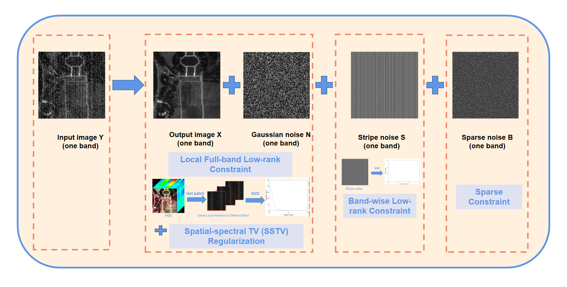
• Previous methods on denoising mixed noise usually classify stripes to sparse noise without considering its structural specificity, while in our paper, we treat the stripes as an independent component and take full advantage of its low-rank property, thus obtaining better destriping and denoising performance.
• A global spatial-spectral total variation (SSTV) regularization is combined with the stripe-spectral low-rank constraint (SSLR) in the proposed HSI denoising model to reconstruct the clean image, stripe, and sparse noise.
• The augmented Lagrange multiplier (ALM) algorithm is employed to solve the proposed SSLR-SSTV model. Both simulated and real data experimental results demonstrate that the proposed method improves the denoising results significantly when compared with the state-of-the-art techniques. Especially, the proposed method provide superb destriping performance with the stripe low-rank constraint.

The rest of the paper is organized as follows. Section 2 introduces the backgrounds and preliminaries on low-rank property of HSI and stripes and SSTV regularization. The proposed denoising model is described in Section 3. Section 4 is the experimental configurations. In Section 5, both simulated experiments and real data experiment are described and analyzed. We analyze the influence of selecting several important parameters in Section 6, and finally, conclusions are given in Section 7.

2. Backgrounds and Preliminaries

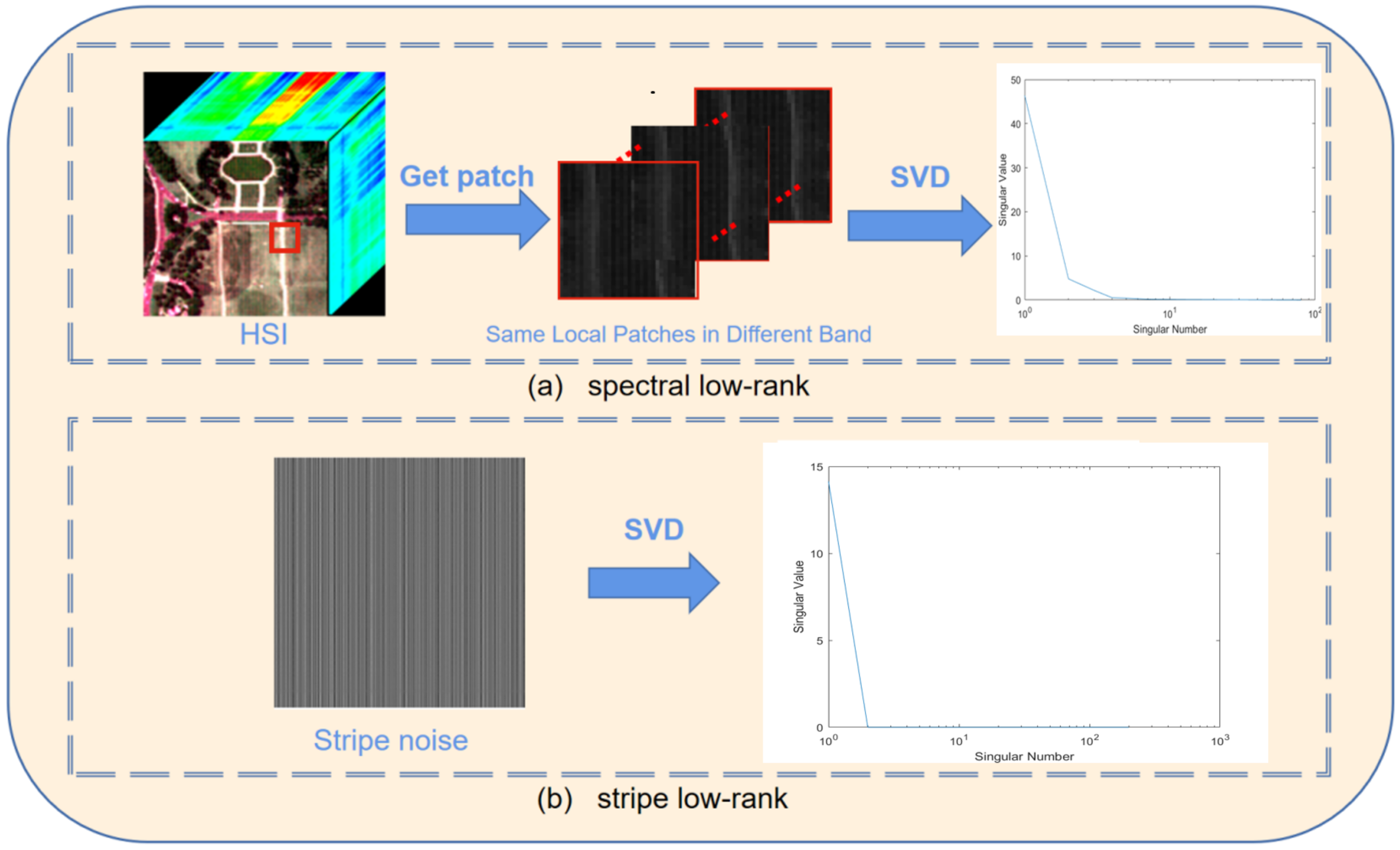
2.1. Low-Rank Property of HSI and Stripe Component

The spectral bands of HSI data are highly correlated and have abundant redundancy. This implies that a large number of spectra can be represented by linear low-dimensional models [28]. To illustrate this property, we extract a full-band image patch of size $m\times n\times P$ from a HSI of size $M\times N\times P$, and convert the patch into a matrix of size $mn\times P$. For analyzing the low-rank property over the bands, we decompose the matrix using the singular value decomposition (SVD), as shown in Figure 1a. The rank of full-band patch is much less than its size, i.e., $r_1\ll P$ and $r_1\ll mn$.

In terms of the stripe noise, it is different from other noise and has significant structural and directional characteristics. We quantitatively analyze the property of stripes in HSI. For a simulated stripe noise image, we decompose the stripe matrix using the SVD, as shown in Figure 1b. We can observe that the singular values of the stripe image rapidly decrease to zero with rank 1. In other words, the subspace of additive stripes can be well modeled by low-rank constraints. Therefore, we propose to use the low-rank constraint on the stripe directly.

2.2. Spatial-Spectral TV (SSTV) Regularization

TV-based techniques have been widely applied to image denoising since its emergence [20]. It helps to regularize the signals while preserving the important details. Without exception, it is one of the most powerful and popular tools for HSI noise removal [14,33,42,43]. For a 2D grayscale image $\mathbf{I}$, the standard isotropic TV norm is defined as

$${\parallel \mathbf{I}\parallel }_{TV}=\parallel D_i{\mathbf{I}\parallel }_1+{\parallel D_j\mathbf{I}\parallel }_1$$

(1)

where $D_i$ and $D_j$ compute the first-order derivative along the horizontal and vertical direction of the input image, respectively. The ${∥·∥}_1$ is L1-norm and denotes the sum of absolute value of the matrix. Note that an HSI has three dimensions and strong correlations between bands. Therefore, the isotropic SSTV norm of an HSI $\mathbf{X}$ is defined as

$${\parallel \mathbf{X}\parallel }_{SSTV}=\parallel D_i{\mathbf{X}\parallel }_1+\parallel D_j{\mathbf{X}\parallel }_1+{\parallel D_b\mathbf{X}\parallel }_1$$

(2)

where $D_b$ acts the same role as $D_i$ and $D_j$ do, but along the spectral direction. As the gradient of different directions on HSI may be different, the istropic SSTV norm Equation (2) can be extended to an anisotropic version:

$${\parallel \mathbf{X}\parallel }_{SSTV}={\tau }_i\parallel D_i{\mathbf{X}\parallel }_1+{\tau }_j\parallel D_j{\mathbf{X}\parallel }_1+{\tau }_b{\parallel D_b\mathbf{X}\parallel }_1$$

(3)

where ${\tau }_i$, ${\tau }_j$, and ${\tau }_b$ are the weighting coefficients in three directions.

3. Stripe-Spectral Low Rank and Spatial-Spectral TV Method

As mentioned before, an HSI contains different kinds of noises. In this paper, we consider the following model:

$$\mathbf{Y}=\mathbf{X}+\mathbf{S}+\mathbf{B}+\mathbf{N}$$

(4)

where $\mathbf{Y}\in {\mathbb{R}}^{M\times N\times P}$ is the observed HSI, with M, N, and P the number of the rows, columns, and bands, respectively. In (4), $\mathbf{X}$ is the desired clean image, $\mathbf{S}$ corresponds to the additive stripe noise; $\mathbf{N}$ denotes the Gaussian noise; and $\mathbf{B}$ represents the sparse noise, including the impulse noise, dead pixels, or lines. Despite the fact that the noises are dependent in raw space, we do not know the prior knowledge about the correlation between different noises. Therefore, in this paper, we assume that the different noises are independently distributed. The aim of denoising is to recover X from Y.

3.1. Proposed Model

As we have analyzed in Section 2.1, the stripe component $\mathbf{S}$ occurs in random bands and has structurally repeated structure that can be described low-rank features. Therefore, we are inspired by using a low-rank constraint on the stripe. For recovering the clean image $\mathbf{X}$ from observed HSI $\mathbf{Y}$, except for the widely used SSTV regularization, we also apply the spectral low-rank constraint as a regularization term. Finally, we use the sparse constraint on sparse noise component $\mathbf{B}$. Therefore, our image reconstruction model is described by

$$\begin{array}{cc}\hfill & \underset{\mathbf{X},\mathbf{S},\mathbf{B}}{\min }rank\left(\mathbf{X}\right)+\lambda {∥\mathbf{B}∥}_1+\tau {∥\mathbf{X}∥}_{SSTV}+\beta \sum _{b=1}^{P}rank\left({\mathbf{S}}_b\right)\hfill \\ \hfill & s.t.{∥\mathbf{Y}-\mathbf{X}-\mathbf{S}-\mathbf{B}∥}_F^2\le \xi ,rank\left(\mathbf{X}\right)\le r_1\hfill \\ \hfill & {∥{\mathbf{Y}}_{\mathbf{b}}-{\mathbf{X}}_{\mathbf{b}}-{\mathbf{S}}_{\mathbf{b}}-{\mathbf{B}}_{\mathbf{b}}∥}_F^2\le \xi ,rank\left({\mathbf{S}}_b\right)\le r_2.\hfill \end{array}$$

(5)

As the rank constraint $rank(·)$ is non-convex, we adopt the nuclear norm ${∥·∥}_{*}$ to replace it, i.e., the sum of the singular values of matrix [44,45]. Therefore, the reconstruction model is reformulated as

$$\begin{array}{cc}\hfill & \underset{\mathbf{X},\mathbf{S},\mathbf{B}}{\min }{∥\mathbf{X}∥}_{*}+\lambda {∥\mathbf{B}∥}_1+\tau {∥\mathbf{X}∥}_{SSTV}+\beta \sum _{b=1}^P{∥{\mathbf{S}}_b∥}_{*}\hfill \\ \hfill & s.t.{∥\mathbf{Y}-\mathbf{X}-\mathbf{S}-\mathbf{B}∥}_F^2\le \xi ,rank\left(\mathbf{X}\right)\le r_1\hfill \\ \hfill & {∥{\mathbf{Y}}_{\mathbf{b}}-{\mathbf{X}}_{\mathbf{b}}-{\mathbf{S}}_{\mathbf{b}}-{\mathbf{B}}_{\mathbf{b}}∥}_F^2\le \xi ,rank\left({\mathbf{S}}_b\right)\le r_2\hfill \end{array}$$

(6)

where $\lambda$, $\tau$, and $\beta$ are the coefficients that controls the sparsity regularizer of noise, SSTV regularizer, and the stripe low-rank regularizer, respectively. Moreover, $r_1$ and $r_2$ are the upper bounds of the low-rank matrix.

When solving the low-rank constraint of the above model, the size of each band $X_b$ of the HSI is elongated from $M\times N$ to $MN\times 1$, so the size of $\mathbf{X}$ becomes $MN\times p$, making $\mathbf{X}$ a very thin matrix. It is proved in [46] that the processing of a very thin matrix may cause parametric blurring because of the limited degrees-of-freedom. Therefore, the application of a global low-rank constraint to the HSI is unfavored. In order to solve this problem, in [41], the authors divide the HSI in local and full-band overlapping patches, thus better preserving the detail information. In this paper, we also apply the low-rank constraint to the local patches, refer to Figure 1a as an example. We obtain full-band patches from the 3-D image $\mathbf{X}$ and sparse noise $\mathbf{B}$. For the stripe noise, we still use the global information. Based on this idea, the optimization problem (6) can be defined as

$$\begin{array}{cc}\hfill & \underset{\mathbf{X},\mathbf{S},\mathbf{B}}{\min }\sum _{ij}({∥{\mathbf{X}}_{\mathbf{ij}}∥}_{*}+\lambda {∥{\mathbf{B}}_{\mathbf{ij}}∥}_1)+\tau {∥X∥}_{SSTV}+\beta \sum _{b=1}^P{∥{\mathbf{S}}_b∥}_{*}\hfill \\ \hfill & s.t.{∥{\mathbf{Y}}_{\mathbf{ij}}-{\mathbf{X}}_{\mathbf{ij}}-{\mathbf{S}}_{\mathbf{ij}}-{\mathbf{B}}_{\mathbf{ij}}∥}_F^2\le \xi ,rank\left(\mathbf{X}\right)\le r_1\hfill \\ \hfill & {∥{\mathbf{Y}}_{\mathbf{b}}-{\mathbf{X}}_{\mathbf{b}}-{\mathbf{S}}_{\mathbf{b}}-{\mathbf{B}}_{\mathbf{b}}∥}_F^2\le \xi ,rank\left({\mathbf{S}}_b\right)\le r_2,\hfill \end{array}$$

(7)

where ${\mathbf{X}}_{\mathbf{ij}}$ and ${\mathbf{B}}_{\mathbf{ij}}$ are the clean image patch and sparse noise patch of $m\times n\times p$ at location $(i,j)$, respectively. The patch cube is extracted by a binary operator $A_{ij}:\mathbf{X}\to {\mathbf{X}}_{\mathbf{ij}}$.

The proposed reconstruction model aims to optimize three variables—$\mathbf{X}$, $\mathbf{S}$, and $\mathbf{B}$—simultaneously, which can be solved via an alternatively minimizing strategy. Next, we will introduce the optimization procedure and solve the optimization problem (7) according to the augmented Lagrange multiplier (ALM) method.

3.2. Optimization Procedure

As mentioned above, we adopt the ALM to solve the minimization problem (7) by introducing three variables $J,W\in {\mathbb{R}}^{M\times N\times P}$ and $U\in {\mathbb{R}}^{M\times N\times P\times 3}$. The optimization problem (7) is then equivalent to

$$\begin{array}{cc}\hfill & \underset{\mathbf{X},\mathbf{S},\mathbf{B},J,W,U}{\min }\sum _{ij}({∥{\mathbf{X}}_{ij}∥}_{*}+\lambda {∥{\mathbf{B}}_{ij}∥}_1)+\tau {∥U∥}_{SSTV}+\beta \sum _{b=1}^P{∥{\mathbf{S}}_b∥}_{*}\hfill \\ \hfill & s.t.{\mathbf{X}}_{ij}=J_{ij},J=W,U=\mathbf{D}W,\hfill \\ \hfill & {∥{\mathbf{Y}}_{ij}-{\mathbf{X}}_{ij}-{\mathbf{S}}_{ij}-{\mathbf{B}}_{ij}∥}_F^2\le \xi ,rank\left(\mathbf{X}\right)\le r_1\hfill \\ \hfill & {∥{\mathbf{Y}}_b-{\mathbf{X}}_b-{\mathbf{S}}_{\mathbf{b}}-{\mathbf{B}}_b∥}_F^2\le \xi ,rank\left({\mathbf{S}}_b\right)\le r_2\hfill \end{array}$$

(8)

where $\mathbf{D}= \left[{\tau }_i{D}_i,{\tau }_j{D}_j,{\tau }_b{D}_b\right]$ is the SSTV operator, as presented in Equation (3).

The augmented Lagrangian function is described as follows:

$$\begin{array}{cc}\hfill & \left\{\mathbf{X},\mathbf{S},\mathbf{B},J,W,U\right\}=\arg \underset{\mathbf{X},\mathbf{S},\mathbf{B},J,W,U}{\min }\sum _{ij}\left({∥{\mathbf{X}}_{ij}∥}_{*}+\lambda {∥{\mathbf{B}}_{ij}∥}_1\right.\hfill \\ \hfill & +{\mathcal{I}}_{ij}^Y·({\mathbf{Y}}_{ij}-{\mathbf{X}}_{ij}-{\mathbf{B}}_{ij}-{\mathbf{S}}_{ij})+\frac{\rho }{2}{∥{\mathbf{Y}}_{ij}-{\mathbf{X}}_{ij}-{\mathbf{B}}_{ij}-{\mathbf{S}}_{ij}∥}_F^2\hfill \\ \hfill & \left.+{\mathcal{I}}_{ij}^X·({\mathbf{X}}_{ij}-J_{ij})+\frac{\rho }{2}{∥{\mathbf{X}}_{ij}-J_{ij}∥}_F^2\right)+{\mathcal{I}}^J·(J-W)+\frac{\rho }{2}{∥J-W∥}_F^2\hfill \\ \hfill & +\tau {∥U∥}_{SSTV}+{\mathcal{I}}^U·(U-\mathbf{D}W)+\frac{\rho }{2}{∥U-\mathbf{D}W∥}_F^2\hfill \\ \hfill & +\sum _{b=1}^P\left(\beta {∥{\mathbf{S}}_b∥}_{*}+{\mathcal{I}}_b^S·({\mathbf{Y}}_b-{\mathbf{X}}_b-{\mathbf{B}}_b-{\mathbf{S}}_b)+\frac{\rho }{2}{∥{\mathbf{Y}}_b-{\mathbf{X}}_b-{\mathbf{B}}_b-{\mathbf{S}}_b∥}_F^2\right)\hfill \end{array}$$

(9)

where $\rho$ is the penalty coefficient, and ${\mathcal{I}}_{ij}^Y$, ${\mathcal{I}}_{ij}^X$, ${\mathcal{I}}^J$, ${\mathcal{I}}^U$, and ${\mathcal{I}}_b^S$ are the Lagrangian multipliers. By choosing proper initialization and regularization parameters, we can obtain a satisfactory result. The restoration process of ALM can be decomposed into six simpler subproblems, and their variables are updated in an alternate iterative manner.

(1) Optimization problem regarding${\mathbf{X}}_{ij}$:

$$\begin{array}{cc}\hfill & {\mathbf{X}}_{ij}=\arg \underset{{\mathbf{X}}_{ij}}{\min }\sum _{ij}\left({∥{\mathbf{X}}_{ij}∥}_{*}+{\mathcal{I}}_{ij}^Y·({\mathbf{Y}}_{ij}-{\mathbf{X}}_{ij}-{\mathbf{B}}_{ij}-{\mathbf{S}}_{ij})+\frac{\rho }{2}{∥{\mathbf{Y}}_{ij}-{\mathbf{X}}_{ij}-{\mathbf{B}}_{ij}-{\mathbf{S}}_{ij}∥}_F^2\right.\hfill \\ \hfill & \left.+{\mathcal{I}}_{ij}^X·({\mathbf{X}}_{ij}-J_{ij})+\frac{\rho }{2}{∥{\mathbf{X}}_{ij}-J_{ij}∥}_F^2\right)\hfill \\ \hfill & =\arg \underset{{\mathbf{X}}_{ij}}{\min }\sum _{ij}\left({∥{\mathbf{X}}_{ij}∥}_{*}+\frac{\rho }{2}{∥{\mathbf{Y}}_{ij}-{\mathbf{X}}_{ij}-{\mathbf{B}}_{ij}-{\mathbf{S}}_{ij}+\frac{{\mathcal{I}}_{ij}^Y}{\rho }∥}_F^2+\frac{\rho }{2}{∥{\mathbf{X}}_{ij}-J_{ij}+\frac{{\mathcal{I}}_{ij}^X}{\rho }∥}_F^2\right).\hfill \end{array}$$

(10)

The step of updating ${\mathbf{X}}_{\mathbf{ij}}$ is a typical low-rank matrix approximation problem, which can be easily solved by performing a soft threshold operation on the matrix singular value decomposition (SVD) [47]:

$$\left\{\begin{array}{c}{\mathbf{X}}_{ij}=U(shrink\_L_{*}({\Sigma }_{r_1},\frac{1}{2\rho }))V^{*}\hfill \\ shrink\_L_{*}({\Sigma }_{r_1},\frac{1}{2\rho })=\mathrm{diag}\{\max ({{\Sigma }_{r_1}}_{ii}-\frac{1}{2\rho },0)\}\hfill \\ SVD(\frac{{\mathbf{Y}}_{ij}+J_{ij}-{\mathbf{B}}_{ij}-{\mathbf{S}}_{ij}}{2}+\frac{{\mathcal{I}}_{ij}^Y-{\mathcal{I}}_{ij}^X}{2\rho })=U\Sigma V^{*}\hfill \end{array}\right.$$

(11)

where ${{\Sigma }_{r_1}}_{ii}$ is the diagonal element of the singular-value matrix ${\Sigma }_{r_1}=\mathrm{diag}\left({\sigma }_i(1<i<r_1)\right)$.

(2) Optimization problem regarding stripe noise${\mathbf{S}}_{\mathbf{b}}$:

Given an image $\mathbf{X}$, sparse noise $\mathbf{B}$, and the optimization equation of striped noise, ${\mathbf{S}}_{\mathbf{b}}$ is as follows:

$$\begin{array}{cc}\hfill & {\mathbf{S}}_{\mathbf{b}}=\arg \underset{{\mathbf{S}}_b}{\min }\sum _{b=1}^P\left(\beta {∥{\mathbf{S}}_b∥}_{*}+{\mathcal{I}}_b^S·({\mathbf{Y}}_b-{\mathbf{X}}_b-{\mathbf{B}}_b-{\mathbf{S}}_b)+\frac{\rho }{2}{∥{\mathbf{Y}}_b-{\mathbf{X}}_b-{\mathbf{B}}_b-{\mathbf{S}}_b∥}_F^2\right)\hfill \\ \hfill & =\arg \underset{{\mathbf{S}}_b}{\min }\sum _{b=1}^P\left(\beta {∥{\mathbf{S}}_b∥}_{*}+\frac{\rho }{2}{∥{\mathbf{Y}}_b-{\mathbf{X}}_b-{\mathbf{B}}_b-{\mathbf{S}}_b+\frac{{\mathcal{I}}_b^S}{\rho }∥}_F^2\right).\hfill \end{array}$$

(12)

Equation (12) can also be easily solved by performing soft threshold operation on the matrix singular values.

$$\left\{\begin{array}{c}{\mathbf{S}}_{\mathbf{b}}=U\left(shrink\_L_{*}({\Sigma }_{r_2},\frac{\beta }{\rho })\right)V^{*}\hfill \\ SVD({\mathbf{Y}}_b-{\mathbf{B}}_b-{\mathbf{X}}_b+\frac{{\mathcal{I}}_b^S}{\rho })=U\Sigma V^{*}\hfill \end{array}\right.,$$

(13)

where ${\Sigma }_{r_2}=\mathrm{diag}\left({\sigma }_i(1<i<r_2)\right)$.

(3) Optimization problem regarding sparse noise${\mathbf{B}}_{ij}$:

Given an image $\mathbf{X}$, stripe noise $\mathbf{B}$, and the optimization equation of sparse noise, ${\mathbf{B}}_{\mathbf{ij}}$ is as follows:

$$\begin{array}{cc}\hfill & {\mathbf{B}}_{ij}=\arg \underset{{\mathbf{B}}_{ij}}{\min }\sum _{ij}\left({∥{\mathbf{B}}_{ij}∥}_1+{\mathcal{I}}_{ij}^Y·({\mathbf{Y}}_{ij}-{\mathbf{X}}_{ij}-{\mathbf{B}}_{ij}-{\mathbf{S}}_{ij})+\frac{\rho }{2}{∥{\mathbf{Y}}_{ij}-{\mathbf{X}}_{ij}-{\mathbf{B}}_{ij}-{\mathbf{S}}_{ij}∥}_F^2\right)\hfill \\ \hfill & =\arg \underset{{\mathbf{B}}_{ij}}{\min }\sum _{ij}\left({∥{\mathbf{B}}_{ij}∥}_1+\frac{\rho }{2}{∥{\mathbf{Y}}_{ij}-{\mathbf{X}}_{ij}-{\mathbf{B}}_{ij}-{\mathbf{S}}_{ij}+\frac{{\mathcal{I}}_{ij}^Y}{\rho }∥}_F^2\right)\hfill \\ \hfill & =shrink\_L_1({\mathbf{Y}}_{ij}-{\mathbf{X}}_{ij}-{\mathbf{S}}_{ij}+\frac{{\mathcal{I}}_{ij}^Y}{\rho },\frac{\lambda }{\rho })\hfill \end{array}$$

(14)

where $shrink\_L_1$ is the soft-threshold operator of L1 norm [48], which is defined as

$$shrink\_L_1(x,\gamma )=\left\{\begin{array}{c}x-\gamma ,ifx>\gamma \hfill \\ x+\gamma ,ifx<\gamma \hfill \\ 0,else\hfill \end{array}\right..$$

(15)

(4) The J-related optimizing step:

$$\begin{array}{c}J=\arg \underset{J}{\min }\sum _{ij}\left({\mathcal{I}}_{ij}^X·({\mathbf{X}}_{ij}-J_{ij})+\frac{\rho }{2}{∥{\mathbf{X}}_{ij}-J_{ij}∥}_F^2\right)+{\mathcal{I}}^J·(J-W)+\frac{\rho }{2}{∥J-W∥}_F^2\hfill \\ =\arg \underset{J}{\min }\sum _{ij}\left(\frac{\rho }{2}{∥{\mathbf{X}}_{ij}-J_{ij}+\frac{{\mathcal{I}}_{ij}^X}{\rho }∥}_F^2\right)+\frac{\rho }{2}{∥J-W+\frac{{\mathcal{I}}^J}{\rho }∥}_F^2.\hfill \end{array}$$

(16)

It is easy to see that (16) has a closed-form solution. The form of solution is as follows:

$$J=(W-\frac{{\mathcal{I}}^J}{\rho }+\sum _{ij}{A}_{ij}^T({\mathbf{X}}_{ij}+\frac{{\mathcal{I}}_{ij}^X}{\rho }))./(L+\sum _{ij}{A}_{ij}^T{A}_{ij})$$

(17)

where L represents a full-one tensor of size $M\times N\times P$, and $./$ means dividing each element of the previous matrix by the corresponding element of the latter matrix.

(5) The W-related optimizing step:

$$\begin{array}{cc}& W=\arg \underset{W}{\min }{\mathcal{I}}^U·(U-\mathbf{D}W)+\frac{\rho }{2}{∥U-\mathbf{D}W∥}_F^2+{\mathcal{I}}^J·(J-W)+\frac{\rho }{2}{∥J-W∥}_F^2\hfill \\ \hfill =& \arg \underset{W}{\min }\frac{\rho }{2}{∥U-\mathbf{D}W+\frac{{\mathcal{I}}^U}{\rho }∥}_F^2+\frac{\rho }{2}{∥J-W+\frac{{\mathcal{I}}^J}{\rho }∥}_F^2.\hfill \end{array}$$

(18)

This problem can be effectively solved according to the fast Fourier transform (FFT) method [41]:

$$W={\mathcal{F}}^{-1}\left[\frac{\mathcal{F}((J+\frac{{\mathcal{I}}^J}{\rho })+{\mathbf{D}}^T(U+\frac{{\mathcal{I}}^U}{\rho }))}{1+\mathcal{F}{({\tau }_i{\mathbf{D}}_i)}^2+\mathcal{F}{({\tau }_j{\mathbf{D}}_j)}^2+\mathcal{F}{({\tau }_b{\mathbf{D}}_b)}^2}\right]$$

(19)

where $\mathcal{F}$ and ${\mathcal{F}}^{-1}$ represent the Fast Fourier Transform (FFT) and the inverse FFT, respectively. ${\mathbf{D}}^T$ stands for the adjoint operator of $\mathbf{D}$.

(6) The U-related optimizing step:

$$\begin{array}{c}U=\arg \underset{U}{\min }\tau {∥U∥}_1+{\mathcal{I}}^U·(U-DW)+\frac{\rho }{2}{∥U-DW∥}_F^2\hfill \\ =\arg \underset{U}{\min }\tau {∥U∥}_1+\frac{\rho }{2}{∥U-DW+\frac{{\mathcal{I}}^U}{\rho }∥}_F^2\hfill \end{array}$$

(20)

where Y and U can be expressed as ${\mathcal{I}}^U=[{\mathcal{I}}_1^U,{\mathcal{I}}_2^U,{\mathcal{I}}_3^U]$ and $U=[U1,U2,U3]$. The optimization problem (20) can be solved by soft-thresholding (shrinkage) operator $shrink\_L_1$, which is the same as Equation (15):

$$\left\{\begin{array}{c}\hfill U_1=shrink\_L_1({\tau }_i{\mathbf{D}}_{i}W-\frac{{\mathcal{I}}_1^U}{\rho },\frac{\tau }{\rho })\\ \hfill U_2=shrink\_L_1({\tau }_j{\mathbf{D}}_{j}W-\frac{{\mathcal{I}}_2^U}{\rho },\frac{\tau }{\rho })\\ \hfill U_3=shrink\_L_1({\tau }_b{\mathbf{D}}_{b}W-\frac{{\mathcal{I}}_3^U}{\rho },\frac{\tau }{\rho })\end{array}\right..$$

(21)

Then, the Lagrangian multipliers ${\mathcal{I}}_{ij}^Y$, ${\mathcal{I}}_{ij}^X$, ${\mathcal{I}}^J$, ${\mathcal{I}}^U$ and ${\mathcal{I}}_b^S$ can be updated in parallel:

$$\left\{\begin{array}{c}{\mathcal{I}}_{ij}^Y={\mathcal{I}}_{ij}^Y+\rho ({\mathbf{Y}}_{ij}-{\mathbf{X}}_{ij}-{\mathbf{B}}_{ij}-{\mathbf{S}}_{ij})\hfill \\ {\mathcal{I}}_{ij}^X={\mathcal{I}}_{ij}^X+\rho ({\mathbf{X}}_{ij}-J_{ij})\hfill \\ {\mathcal{I}}^J={\mathcal{I}}_{ij}^J+\rho (J-W)\hfill \\ {\mathcal{I}}^U={\mathcal{I}}_{ij}^U+\rho (U-\mathbf{D}W)\hfill \\ {\mathcal{I}}_b^S={\mathcal{I}}_{ij}^S+\rho ({\mathbf{Y}}_b-{\mathbf{X}}_b-{\mathbf{B}}_b-{\mathbf{S}}_b)\hfill \end{array}\right..$$

(22)

The algorithm procedure is summarized in Algorithm 1.

Algorithm 1 SSLR-SSTV

1:   Input: observed HSI $\mathbf{Y}$, desired rank r, patch size, stopping criterion $\epsilon$, regularization parameters

$\lambda$, $\beta$ and $\tau =[{\tau }_i,{\tau }_j,{\tau }_b]$

2:   Initialize: Set parameters $\lambda$, $\beta$, $\tau =[{\tau }_i,{\tau }_j,{\tau }_b]$, $\epsilon$, r; $\mathbf{Y}$ = $\mathbf{X}$ = J = W; U = $\mathbf{S}$ = $\mathbf{B}$ = 0;

3:   for iter=1: IterMax do

Update ${\mathbf{X}}_{\mathbf{ij}}$ via (11);

Compute ${\mathbf{S}}_{\mathbf{b}}$ by solving (13);

Solve (14) for $\mathbf{B}$;

Update J, W, U, and the Lagrangian multipliers using (17), (19), (21) and (22), respectively.

Check the convergence conditions.

${∥\mathbf{Y}-\mathbf{X}-\mathbf{S}-\mathbf{B}∥}_F^2\le \xi$,

${∥{\mathbf{Y}}_{\mathbf{b}}-{\mathbf{X}}_{\mathbf{b}}-{\mathbf{S}}_{\mathbf{b}}-{\mathbf{B}}_{\mathbf{b}}∥}_F^2\le \xi$

end for

4:   Output: Clean Image $\mathbf{X}$, sparse noise $\mathbf{B}$ and stripe noise $\mathbf{S}$.

4. Experimental Configurations

4.1. Datasets

In our experiments, we use four HSI datasets. The details of these datasets (The datasets are available through: http://lesun.weebly.com/hyperspectral-data-set.html, https://engineering.purdue.edu/biehl/MultiSpec/hyperspectral.html, http://www.escience.cn/people/feiyunZHU/DatasetGT.html (accessed on 11 January 2021)) are as follows.

• ROSIS Pavia city center dataset: This dataset was collected by the reflective optics system imaging spectrometer (ROSIS-03). We use a $200\times 200\times 80$ cube to implement our experiment.
• HYDICE Washington DC Mall (WDC) dataset: This dataset was acquired in the Washington DC mall by the Hyperspectral Digital Imagery (HYDICE) sensor. The whole image contains $1208\times 307$ pixels and 191 spectral channels. We select a sub-image of $256\times 256\times 80$.
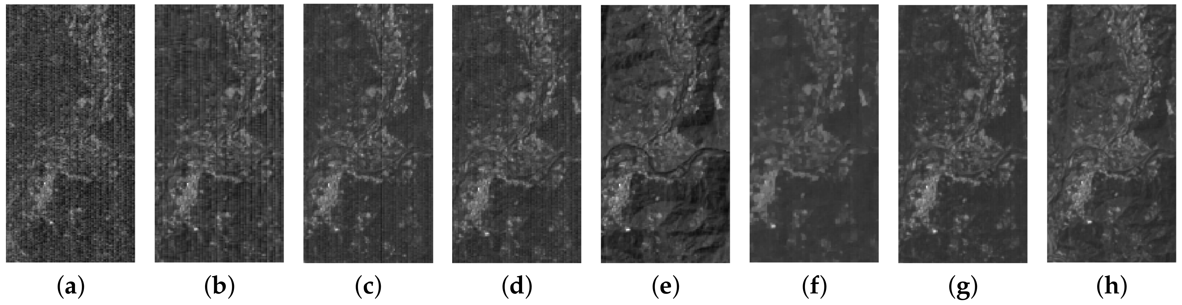
• EO Hyperion Dataset: This dataset was acquired by the EO-1 HYPERION sensor; the spectral and spatial resolutions of this dataset are 166 bands and $400\times 200$ pixels, respectively.
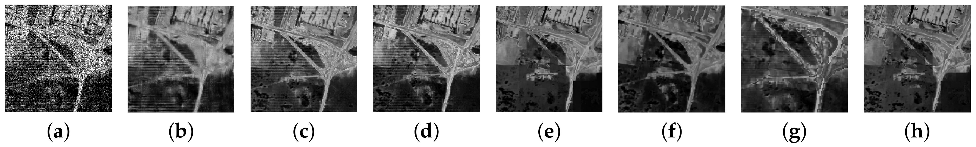
• HYDICE Urban Dataset: This dataset was acquired in the Copperas Cove by the HYDICE sensor, which also contains intricate ground substances. The spectral and spatial resolutions of this dataset are 210 bands and $307\times 307$ pixels.

The first two datasets are noise-free and used in the simulated experiments. The last two datasets are corrupted by real noise and used in the real noise experiments.

4.2. Experimental Indicators and Settings

In the simulated experiments, we use the mean peak signal-to-noise ratio (MPSNR) [49,50], mean structural similarity (MSSIM) [51], and the mean spectral angle mapper (MSAM) [52] to evaluate the quality of the denoising results of each algorithm. PSNR and SSIM are two of the most widely used quality assessment indexes in the field of image processing and computer vision. The PSNR measures the quality of the restored image according to the mean square error, and the SSIM evaluates the similarity between the target image and the reference image. The higher the PSNR and SSIM are, the better the restored image is. SAM calculates the spectral similarity according to the angular difference between the spectrum vectors of the filtered and the noise-free HSI. The smaller SAM is, the more similar the restored image is to the original image. These three measurements are calculated as

$$\begin{array}{c}MPSNR=\frac{1}{b}\sum _{b=1}^{P}10lo{g}_{10}\frac{{I_{max,b}}^2\times MN}{{∥{\widehat{u}}_b-u_b∥}^2}\hfill \\ MSSIM=\frac{1}{b}\sum _{b=1}^P\frac{(2{\mu }_{u_b}{\mu }_{{\widehat{u}}_b}+C_1)(2{\sigma }_{u_b{\widehat{u}}_b}+C_2)}{({\mu }_{u_b}^2+{\mu }_{{\widehat{u}}_b}^2+C_1)({\sigma }_{u_b}^2+{\sigma }_{{\widehat{u}}_b}^2+C_2)}\hfill \\ MSAM=\frac{1}{P}\sum _{b=1}^{P}arccos\left[\frac{{\sum }_i^{MN}{u}_b^i{\widehat{u}}_b^i}{\sqrt{{\sum }_{i=1}^{MN}{(u_b^i)}^2}\sqrt{{\sum }_{i=1}^{MN}{({\widehat{u}}_b^i)}^2}}\right]\hfill \end{array}$$

(23)

where $I_{max,b}$ is the maximum value of the image on the $b_{th}$ band. ${\widehat{u}}_b$ and $u_b$ denote the denoised and clean HSI in $b_{th}$ band, respectively. ${\mu }_{u_b}$ and ${\mu }_{{\widehat{u}}_b}$ are average values of image $u_b$ and ${\widehat{u}}_b$, and ${\sigma }_{u_b}$, ${\sigma }_{{\widehat{u}}_b}$ represent the the variances, while ${\sigma }_{u_b{\widehat{u}}_b}$ means the covariance between two images.

In real HSI experiments, due to the lack of reference image, we use a no-reference HSI quality assessment (The MATLAB code was provided by Dr. Jingxiang Yang; Available: https://github.com/polwork/No-Reference-Hyperspectral-Image-Quality-Assessment-via-Quality-Sensitive-Features-Learning (accessed on 11 January 2021)) [50] to evaluate the denoised images. The smaller the quality assessment score is, the better the denoising or restoring result is.

In both simulated and read data experiments, we compare our denoising results with six state-of-the-art denoising methods on mixed noise: BM4D [12], low-rank matrix recovery (LRMR) [25], the TV-regularized low-rank method (LRTV) [33], the noise-adjusted iterative low-rank matrix approximation (NAILRMA) [26], SSTV-regularized local low-rank matrix recovery (LLRSSTV) he2018hyperspectral, and double-factor-regularized LRTF (LRTF-DFR) method [34]. In addition, in order to further demonstrate the superior destriping performance of our method, we also compare our SSLR-SSTV method with the low-rank-based single-image decomposition model (LRID) under different stripe noise.

We set the penalty parameter $\rho$ as ${10}^{-2}$. The patch size is initialized to $20\times 20$, and the step length is 10 both in the horizontal and vertical directions, empirically. Finally, the stopping criterion $\epsilon$ and the iteration number IterMax are set to ${10}^{-6}$ and 50, respectively. Before the denoising, we normalize the HSI data to [0, 1] by dividing the maximal value of the HSI data cube. The selection of parameters will be discussed in Section 6.

4.3. Simulation Configurations

Real HSIs are usually degraded by a mix of various noises. The goal of our algorithm is to destripe and denoise. To simulate a noisy image, we add Gaussian noise with different standard variance $\sigma$, salt-and-pepper impulse noise with different percentage o, and stripes with different percentages r and different intensities v to randomly selected $30\%$ the bands of the two HSI datasets, as described in the following three cases.

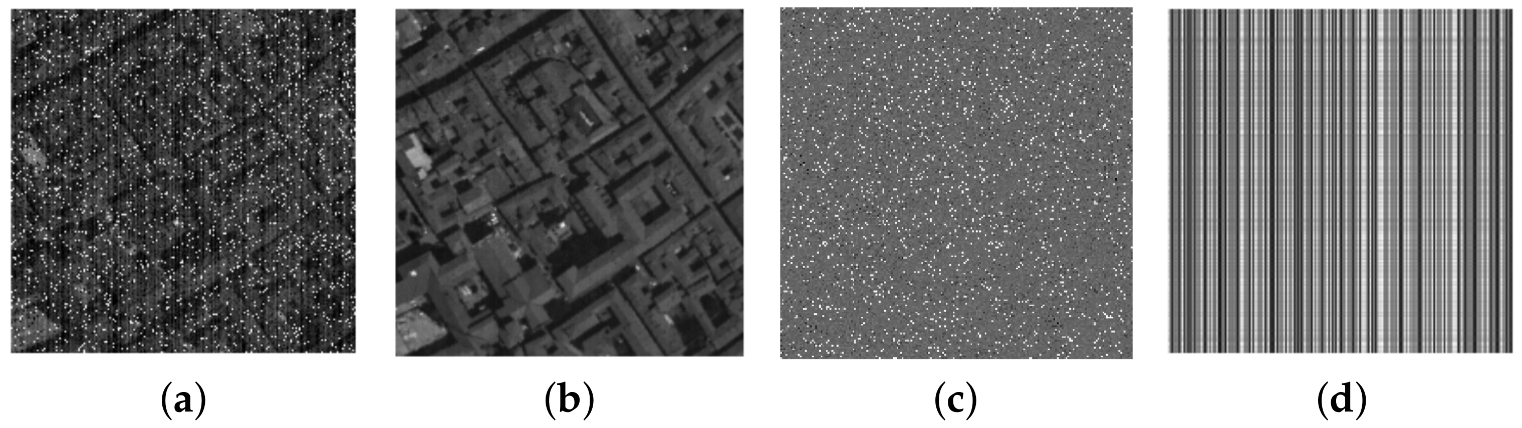
• Case 1: (Gaussian Noise + Salt and Pepper Noise + stripes with different percentages) We add Gaussian noise and impulse noise with $\sigma$ = 0.05 and o = 0.1. Besides, the intensity of the stripes is $v=0.075$. For each band with stripes, we consider using increasing percentages of the stripes r = 0.3, 0.5, and 0.7, respectively.
• Case 2: (Gaussian Noise + Salt and Pepper Noise + stripes with different intensity) Based on case 1, we choose the stripe noise with the percentage of r = 0.3 and the intensity of v = 0.05, 0.075, and 0.1.
• Case 3: (only stripes) Only stripe noise is added to image data. The intensity of the stripes is v = 0.05 0.075, 0.1, and the percentages of the stripes are r = 0.3, 0.5.

5. Experimental Results

In this part, we conduct several simulated and real data experiments to verify the effectiveness of our method.

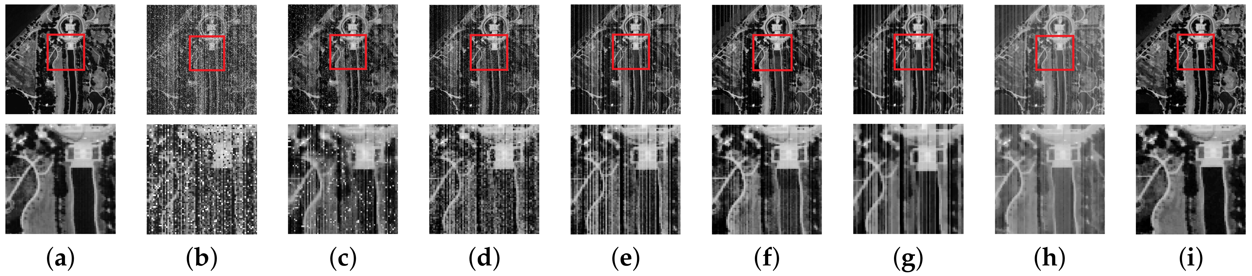
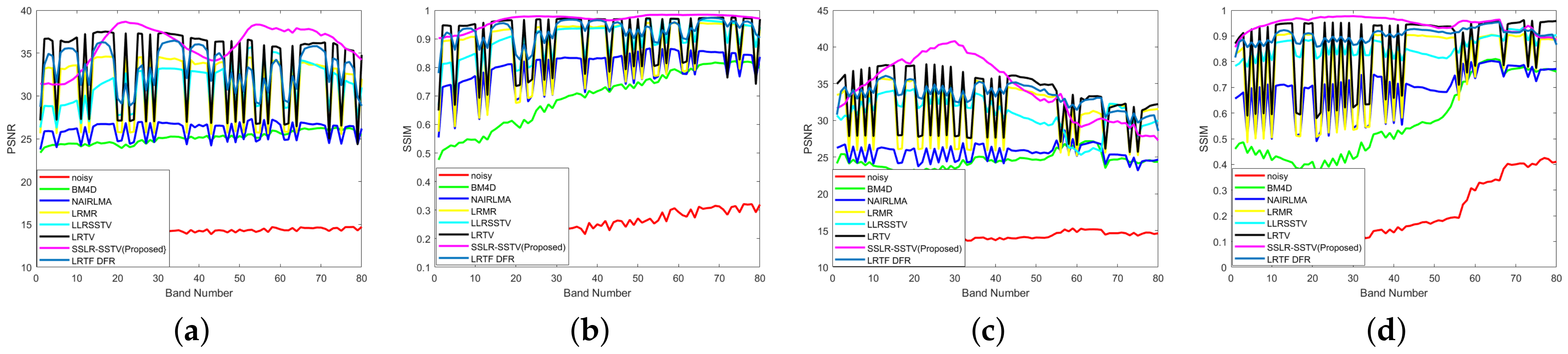
5.1. Simulated Data Experiments

In our proposed method, clean image components $\mathbf{X}$ are reconstructed through TV regularization terms and local low-rank constraints. The $L_1$ sparse regularization and the low-rank constraint help to separate the sparse noise $\mathbf{B}$ and stripe noise $\mathbf{S}$ from the HSI, respectively. Figure 2 illustrates the output independent components of our method in case 1 with $\sigma$ = 0.05, o = 0.1, v = 0.075, and r = 0.3. Figure 2a presents the observed image $\mathbf{Y}$, Figure 2b is the denoised image $\mathbf{X}$, and Figure 2c,d shows the output sparse noise $\mathbf{B}$ and the output stripe noise $\mathbf{S}$, respectively.

Figure 3 and Figure 4 present the denoising results of the different methods for the two simulated data sets in Case 1 with r = 0.5, v = 0.075. Figure 3 shows the denoising results of Pavia city center data in band 11 and its zoom-in image. Figure 4 presents the denoising results of Washington DC Mall data in band 3 and its zoom-in image. Figure 3a and Figure 4a present the original Pavia City Center data and Washington DC Mall data, respectively. Figure 3b and Figure 4b show the image after adding the simulated mixed noise. Figure 3c–i and Figure 4c–i display the denoising results of the different methods. By visually comparing the denoising results of these methods, it can be seen clearly that the proposed method outperforms the other methods and can effectively remove the mixed noise. From Figure 4c–i, we can observe that BM4D fails in removing sparse noise and stripe noise because it does not consider the correlation between bands. NAILRMA does not behave well because it only considers the Gaussian distribution of noise. LRMR, LLRSSTV, LRTV, and LRTF-DFR can effectively remove the sparse noise and Gaussian noise, but the stripe noise is not well filtered. Figure 3 and Figure 4 demonstrate that the proposed SSLR-SSTV can best preserve local details and remove high intensity of stripe noises in the mixed noise.

Figure 5 shows the PSNR and SSIM values of each band of the Pavia City Center images and Washington DC Mall in case 1, respectively. As presented in Figure 5, the proposed method achieves the best PSNR and SSIM values in most bands of the image. In addition, we can see that the PSNR and SSIM of our method are smooth between bands, while other methods have relatively large differences between each band, which forms sawtooth. Actually, the sawtooth is generated at bands where there are stripe noise. Figure 5 proves that our method has better destriping performance than the other methods. The above experiments demonstrate the superiority of the proposed method, especially its ability of destriping in mixed noise.

The quantitative evaluation results of the different denoising methods with the simulated noise in cases 1 and 2 for the Washington DC Mall data and the Pavia City Center data are shown in

Table 1. In the different cases of simulated mixed noise (case 1 and case 2), the quantitative picture quality indices of denoising two HSI data with different methods.

Case	Data	Gaussian Noise	Salt and Pepper Noise	Stripes	Indicators	Noisy	BM4D	NAILRMA	LRMR	LLRSSTV	LRTV	LRTF_DFR	SSLR-SSTV
Case 1 Gaussian+ Salt and Pepper Noise +stripes (different percentages)	Pavia city	$\sigma$ = 0.05	o = 0.1	r = 0.3 v = 0.075 r = 0.5 v = 0.075 r = 0.7 v = 0.075	MPSNR MSSIM MSAM MPSNR MSSIM MASM MPSNR MSSIM MSAM	14.2135 0.2414 0.7083 14.1624 0.2380 0.7103 14.1338 0.2358 0.7126	25.1773 0.6985 0.2340 25.0946 0.6944 0.2325 25.0585 0.6914 0.2339	26.3919 0.8161 0.1415 25.9381 0.7916 0.1569 25.5457 0.7627 0.1805	32.1789 0.9006 0.1442 31.3789 0.8760 0.1746 30.9459 0.8468 0.2099	33.0750 0.9256 0.1299 31.0370 0.8924 0.1634 30.0624 0.8564 0.2102	34.0848 0.9240 0.1311 33.5149 0.9078 0.1566 33.1073 0.8819 0.1922	34.2962 0.9400 0.1001 33.3251 0.9286 0.1062 32.6091 0.9028 0.1062	35.9412 0.9672 0.0883 35.9781 0.9674 0.0860 35.9542 0.9674 0.0864
	Washington DC Mall	$\sigma$ = 0.05	o = 0.1	r = 0.3 v = 0.075 r = 0.5 v = 0.075 r = 0.7 v = 0.075	MPSNR MSSIM MSAM MPSNR MSSIM MASM MPSNR MSSIM MSAM	14.1100 0.2030 0.6104 14.0866 0.2013 0.6127 14.0452 0.1989 0.6145	24.5282 0.5682 0.2187 24.5261 0.5675 0.2198 24.3282 0.5574 0.2213	25.9672 0.7230 0.1597 25.5618 0.6864 0.1708 25.2558 0.6745 0.1769	32.2587 0.8481 0.1017 31.3062 0.8015 0.1255 31.2042 0.7979 0.1400	32.2334 0.8989 0.1162 30.9260 0.8584 0.1302 30.6388 0.8407 0.1283	33.4941 0.8946 0.0746 32.7237 0.8561 0.0939 32.5230 0.8466 0.1102	34.7571 0.9327 0.0577 33.5054 0.9059 0.0668 33.1975 0.8954 0.6070	34.7809 0.9499 0.0807 34.6840 0.9494 0.0806 34.7539 0.9498 0.0795
Case 2 Gaussian+ Salt and Pepper Noise +stripes (different intensity)	Pavia city	$\sigma$ = 0.05	o = 0.1	r = 0.3 v = 0.05 r = 0.3 v = 0.1	MPSNR MSSIM MSAM MPSNR MSSIM MSAM	14.2506 0.2445 0.7061 14.1672 0.2387 0.7110	25.2494 0.7020 0.2333 25.0163 0.6935 0.2359	26.6699 0.8329 0.1333 25.8698 0.7903 0.1612	33.2249 0.9298 0.1187 31.3262 0.8757 0.1695	35.0842 0.9585 0.0909 31.1318 0.8958 0.1570	34.9714 0.9478 0.1072 33.4429 0.9053 0.1485	35.6133 0.9619 0.0765 33.0726 0.9218 0.1217	35.9348 0.9673 0.0881 35.9719 0.9676 0.0862
	Washington DC Mall	$\sigma$ = 0.05	o = 0.1	r = 0.3 v = 0.05 r = 0.3 v = 0.1	MPSNR MSSIM MSAM MPSNR MSSIM MASM	14.1461 0.2052 0.6086 14.0768 0.2010 0.6129	24.5298 0.5706 0.2202 24.4740 0.5656 0.2206	26.1667 0.7390 0.1568 25.4846 0.6844 0.1719	33.2962 0.8821 0.0865 31.2627 0.8073 0.1228	32.9514 0.9181 0.1097 30.8719 0.8577 0.1273	34.2894 0.9222 0.0613 32.6464 0.8604 0.0900	35.2569 0.9398 0.0532 33.2457 0.9033 0.0678	34.8278 0.9501 0.0796 34.7806 0.9502 0.0799

. We use bold to mark the best result for each quality index in the same case. As is shown in Table 1, our method achieves the highest MPSNR, the largest MSSIM, and the smallest MSAM in most cases when compared to the other methods. This result proves the advantage of our method in removing mixed noise from HSI.

Besides, we made rough comparisons with three deep learning-based methods [35,36,37]. Given the input images with the same noise level, our method can yield comparable or even better denoising results according to the evaluation indexes. However, we cannot conclude that our method is better than the deep learning-based methods, as those deep learning-based methods need proper training datasets, hyperparameter selection, etc., which are not accessible in our experiments. In this paper, we focus on developing a model-based HSI denoising method to quickly obtain accurate results without supervising information and training data.

Table 2. The result of HSI denoising using low-rank-based single-image decomposition model (LRID) and SSLR-SSTV in different stripe noise levels.

Image	Method	Indicators	Stripes
			r = 0.3 v = 0.075	r = 0.5 v = 0.075	r = 0.7 v = 0.075	r = 0.3 v = 0.05	r = 0.3 v = 0.1
Pavia city	LRID_destripe	MPSNR MSSIM MSAM	32.7530 0.9554 0.0907	32.7487 0.9559 0.0905	32.6235 0.9547 0.0920	33.3185 0.9567 0.0797	32.7800 0.9552 0.0919
	SSLR-SSTV	MPSNR MSSIM MSAM	35.7038 0.9673 0.0866	36.3639 0.9704 0.0805	32.9474 0.9391 0.1048	38.0868 0.9786 0.0722	37.5613 0.9770 0.0753
Washington DC Mall	LRID_destripe	MPSNR MSSIM MSAM	31.9562 0.9403 0.0589	32.0484 0.9394 0.0566	31.8708 0.9403 0.0589	32.0538 0.9404 0.0575	31.8131 0.9392 0.0598
	SSLR-SSTV	MPSNR MSSIM MSAM	33.8812 0.9466 0.0755	36.4991 0.9699 0.0657	33.1961 0.9305 0.0815	35.4121 0.9652 0.0699	33.8284 0.9485 0.0761

shows the destriping results for both Pavia City and Washington DC datasets with the simulated stripe noise in cases 3. In general, our method has higher MPSNR and MSSIM values in most cases compared with the LRID method. This phenomenon shows that our method is competitive in restoring images corrupted by stripe noise. We show the destriping results of the Pavia city and Washington DC Mall in Figure 6 and Figure 7, respectively.

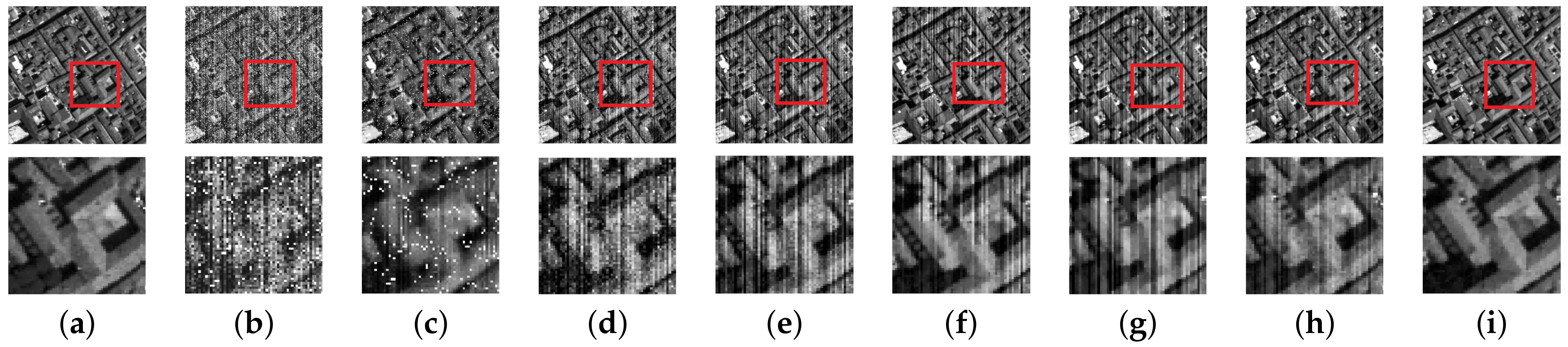
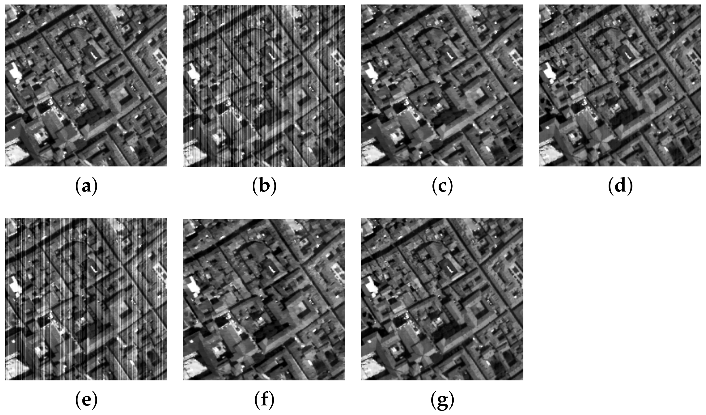
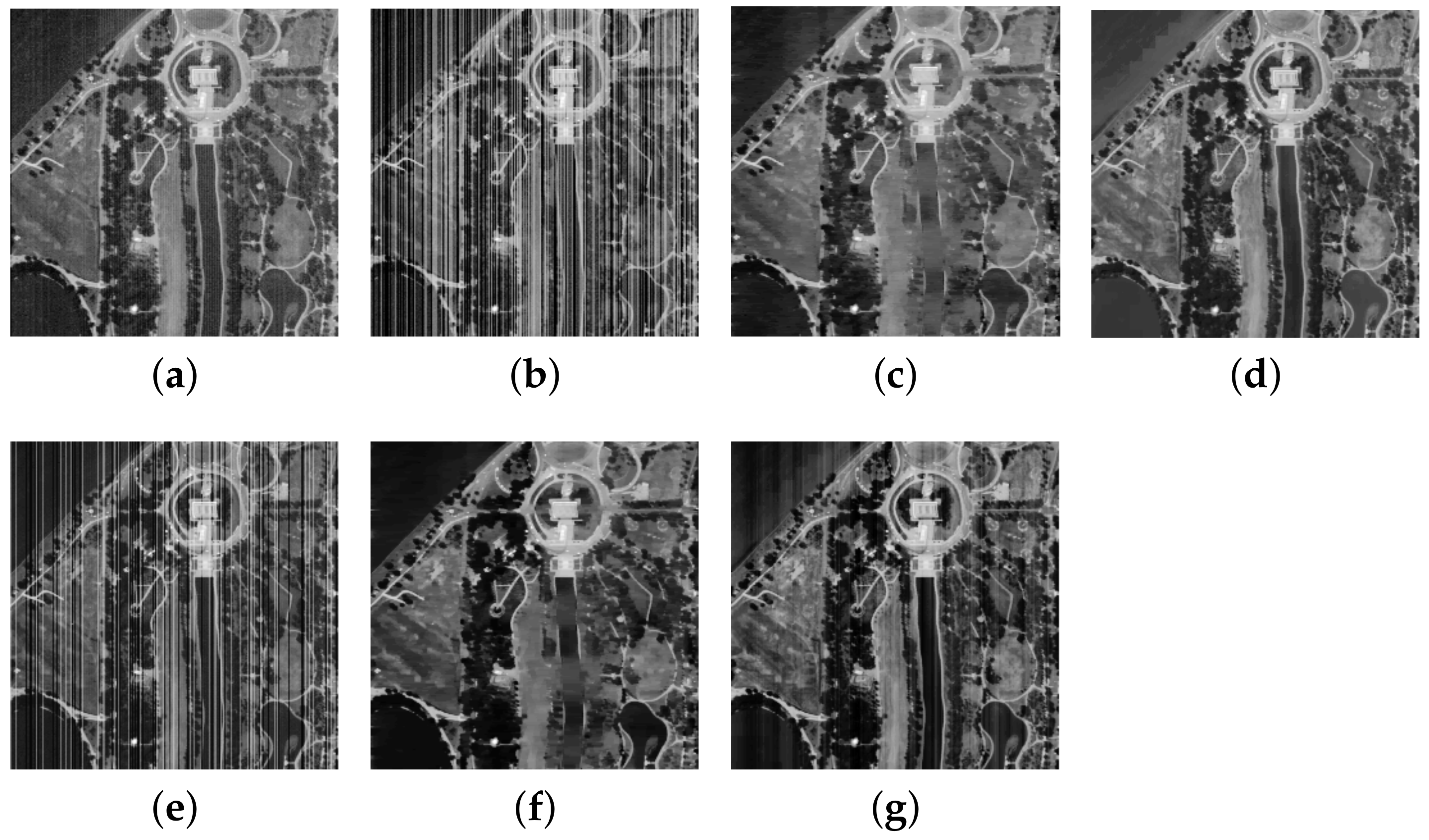
5.2. Real HSI Noise Experiments

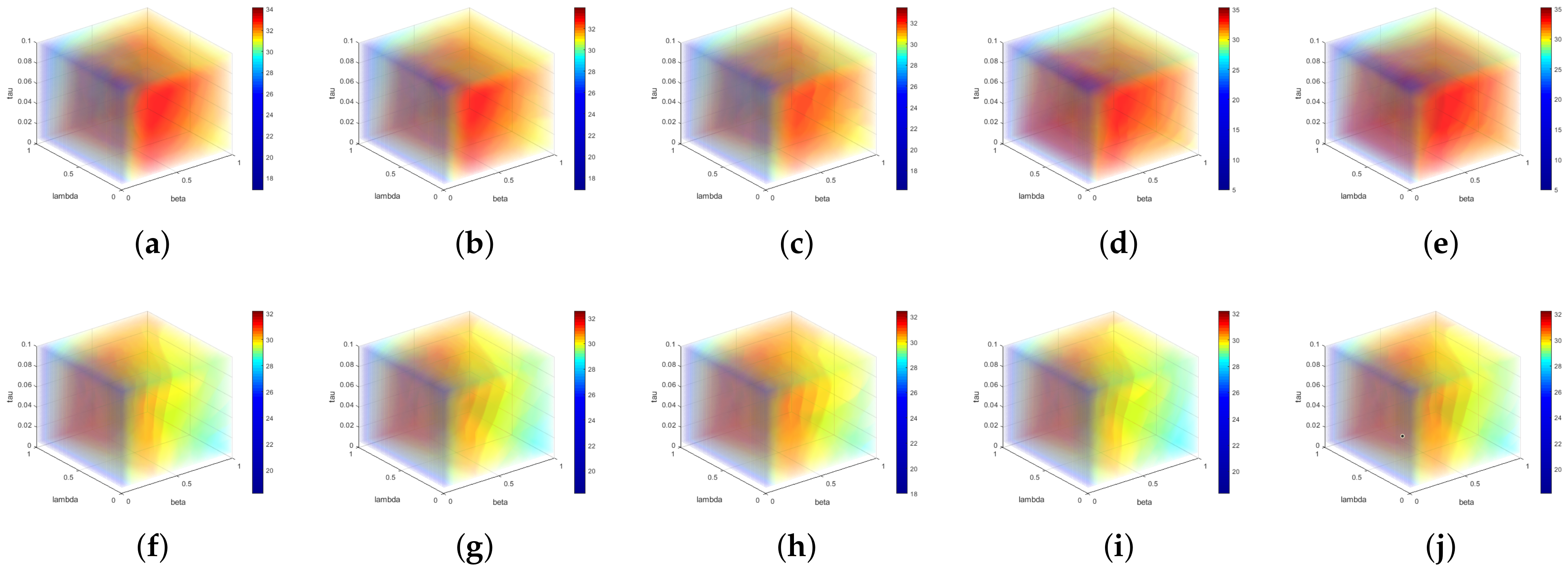
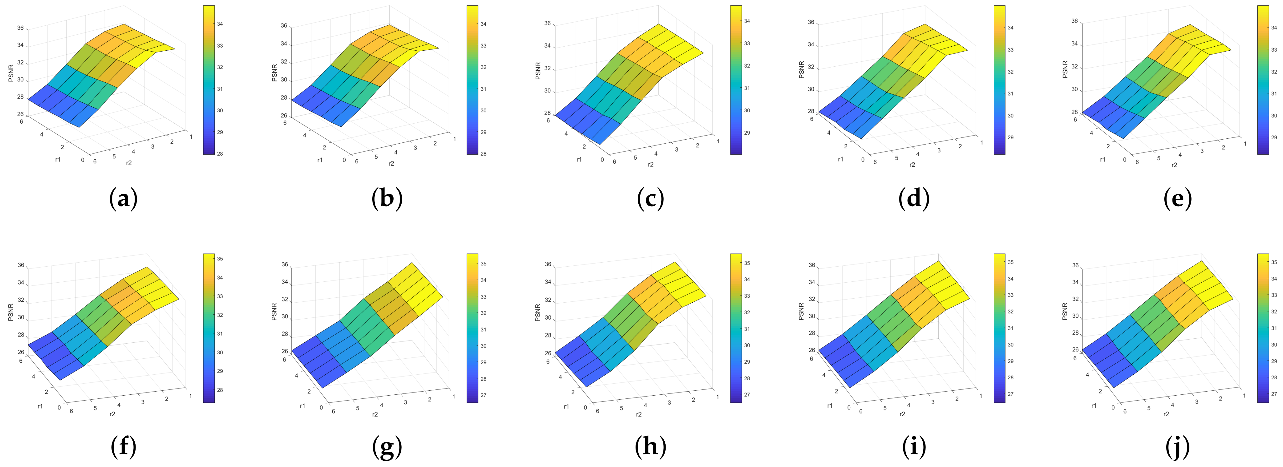
In this section, we evaluate the performance of the proposed method on two real HSI data sets: EO Hyperion Dataset and HYDICE Urban Dataset. Figure 8 and Figure 9 show the denoising results obtained in the EO Hyperion data of bands 132 and Urban dataset of bands 206, respectively. From Figure 8a–h and Figure 9a–h, we can see that the BM4D method fails to denoise the mixed noise. As presented in Figure 8 and Figure 9c,d, the NAILRMA and LRMR can remove some noise, but there is still obvious noise surviving. In Figure 8e and Figure 9e, LRTV has oversmoothed the image and distorted the edge. By comparison, our method, LLRSSTV, and LRTF-DFR achieve a better restoration result visually than other compared methods. In Figure 8e,g, LLRSSTV is slightly better than our method in maintaining details.

Table 3. THE result of HSI denoising on real data.

Data	Noise	BM4D	NAIRLMA	LRMR	LLRSSTV	LRTV	LRTF_DFR	SSLR-SSTV
EO Hyperion	13.7319	13.7218	13.6193	13.4800	12.3797	12.3925	13.4411	12.1580
URBAN	12.9954	12.8967	12.2262	12.2081	10.8188	11.8250	12.9058	10.7117

shows the blind HSI quality assessment of different methods on real data. As shown in this table, our method achieves the lowest scores on two real HSI datasets. This result further demonstrates the superiority and robustness of our method.

6. Discussion

Parameters play significant roles in controlling the denoising performance. In our method, the parameter $\lambda$ controls the regularization of the sparse noise $\mathbf{B}$, $\beta$ is the parameter for stripe noise $\mathbf{S}$, and $\tau$ adjusts the spatial-spectral smoothness of the reconstructed $\mathbf{X}$. In the experiments, we adjust these parameters to achieve the highest PSNR value.

First, we analyze the influence of the parameters $\tau$, $\lambda$ and $\beta$ on the denoising results with the simulated noise in cases 1 and 2 for the two simulated datasets. Figure 10 shows the MPSNR values of SSLR-SSTV on the Pavia dataset and Washington DC Mall data, as related to parameters $\tau$, $\lambda$, and $\beta$. It can be seen from these figures that the optimal parameters of our method are $\tau =0.03$, $\lambda =0.3$ and $\beta =1$, and the result is robust under different noise cases and different images.

Second, we investigate the effect of the upper bound rank $r_1$ and $r_2$. We select $r_1$ and $r_2$ from [1, 6], and fix the parameters as $\tau =0.03$, $\lambda =0.3$ and $\beta =1$. It is clear that the denoised results are best when $r_1=2$ and $r_2=1$ in Figure 11. This is in accordance with our analysis in Section 2.1.

During the simulation experiment, we find some bias between the mean value of the filtered result and the original image, i.e., the filtered image is visually darker than the original image. This phenomenon is because our algorithm regards horizontal and vertical components of the clean image as stripes. Numerous experiments have shown that the difference between the mean value of the filtered image and the original image is close to the mean value of the stripes component. Therefore, we compensate for the filtered result by adding the difference and achieve an excellent visual effect.

Furthermore, we compare the running time with the other methods.

Table 4. Comparisons of computational time for the denoising methods (in seconds).

Data	BM4D	NAILRMA	LRMR	LLRSSTV	LRTV	LRTF_DFR	SSLR-SSTV
Pavia city	178.59 s	60.94 s	111.18	154.63 s	20.94 s	71.22 s	220.25 s
Washington DC Mall	341.22 s	77.57 s	283.32	373.11 s	31.52 s	107.29 s	576.58 s
EO Hyperion	1432.84 s	1951.05 s	1031.03	723.98 s	91.54 s	144.56 s	1006.70 s
URBAN	3526.43 s	4860.03 s	3124.84 s	773.26 s	106.78 s	161.74 s	757.68 s

shows the average processing time of these methods on simulated data and on real data. All of the compared algorithms are running on Matlab R2019a (Intel i7 CPU at 3.60 GHz, 16 GB of memory). Note that our degradation model contains four components, and the optimization process may be a little more costly than the other methods, but our method can provide better denoising and destriping results.

7. Conclusions

Focusing on the destriping and denoising problem of HSI corrupted by mixed noise, we proposed a stripe and spectral low-rank matrix recovery and global spatial-spectral total variation (SSLR-SSTV) method in this paper. In our model, the noises in HSI are classified into sparse noise, stripe noise, and Gaussian noise. A global spatial-spectral TV regularization and local low-rank constraint is utilized to remove the Gaussian noise and reconstruct the clean image. Considering the significant structural and directional characteristic of stripes, we use the low-rank constraint on the stripe noise of each band. In addition, we take advantage of the sparse property to remove the sparse noise. The designed restoration model is efficiently solved by the augmented Lagrange multiplier algorithm. Experiments on both simulated and real HSI datasets show that our method has the ability to accurately suppress noise and keep image details. Our method outperforms the state-of-the-art methods both in visual quality and evaluation criteria, especially when the stripe noise is strong in the mixed noise.

References

1. Landgrebe, D. Hyperspectral image data analysis. IEEE Signal Process. Mag. 2002, 19, 17–28. [Google Scholar] [CrossRef]
2. Ghamisi, P.; Yokoya, N.; Li, J.; Liao, W.; Liu, S.; Plaza, J.; Rasti, B.; Plaza, A. Advances in hyperspectral image and signal processing: A comprehensive overview of the state of the art. IEEE Geosci. Remote Sens. Mag. 2017, 5, 37–78. [Google Scholar] [CrossRef] [Green Version]
3. Zhang, L.; Zhang, L.; Tao, D.; Huang, X. On combining multiple features for hyperspectral remote sensing image classification. IEEE Trans. Geosci. Remote Sens. 2011, 50, 879–893. [Google Scholar] [CrossRef]
4. Zhou, J.; Kwan, C.; Ayhan, B.; Eismann, M.T. A novel cluster kernel RX algorithm for anomaly and change detection using hyperspectral images. IEEE Trans. Geosci. Remote Sens. 2016, 54, 6497–6504. [Google Scholar] [CrossRef]
5. Yang, J.; Zhao, Y.Q.; Chan, J.C.W. Learning and transferring deep joint spectral–spatial features for hyperspectral classification. IEEE Trans. Geosci. Remote Sens. 2017, 55, 4729–4742. [Google Scholar] [CrossRef]
6. Wang, Q.; Yuan, Z.; Du, Q.; Li, X. GETNET: A general end-to-end 2-D CNN framework for hyperspectral image change detection. IEEE Trans. Geosci. Remote Sens. 2018, 57, 3–13. [Google Scholar] [CrossRef] [Green Version]
7. Rasti, B.; Scheunders, P.; Ghamisi, P.; Licciardi, G.; Chanussot, J. Noise reduction in hyperspectral imagery: Overview and application. Remote Sens. 2018, 10, 482. [Google Scholar] [CrossRef] [Green Version]
8. Elad, M. On the origin of the bilateral filter and ways to improve it. IEEE Trans. Image Process. 2002, 11, 1141–1151. [Google Scholar] [CrossRef] [Green Version]
9. Buades, A.; Coll, B.; Morel, J.M. A non-local algorithm for image denoising. In Proceedings of the 2005 IEEE Computer Society Conference on Computer Vision and Pattern Recognition (CVPR’05), San Diego, CA, USA, 20–26 June 2005; Volume 2, pp. 60–65. [Google Scholar]
10. Dabov, K.; Foi, A.; Katkovnik, V.; Egiazarian, K. Image denoising by sparse 3-D transform-domain collaborative filtering. IEEE Trans. Image Process. 2007, 16, 2080–2095. [Google Scholar] [CrossRef] [PubMed]
11. Qian, Y.; Shen, Y.; Ye, M.; Wang, Q. 3-D nonlocal means filter with noise estimation for hyperspectral imagery denoising. In Proceedings of the 2012 IEEE International Geoscience and Remote Sensing Symposium, Munich, Germany, 22–27 July 2012; pp. 1345–1348. [Google Scholar]
12. Maggioni, M.; Katkovnik, V.; Egiazarian, K.; Foi, A. Nonlocal transform-domain filter for volumetric data denoising and reconstruction. IEEE Trans. Image Process. 2012, 22, 119–133. [Google Scholar] [CrossRef]
13. Chen, G.; Bui, T.D.; Quach, K.G.; Qian, S.E. Denoising hyperspectral imagery using principal component analysis and block-matching 4D filtering. Can. J. Remote Sens. 2014, 40, 60–66. [Google Scholar] [CrossRef]
14. Yuan, Q.; Zhang, L.; Shen, H. Hyperspectral image denoising employing a spectral—Spatial adaptive total variation model. IEEE Trans. Geosci. Remote Sens. 2012, 50, 3660–3677. [Google Scholar] [CrossRef]
15. Yuan, Q.; Zhang, L.; Shen, H. Hyperspectral image denoising with a spatial—Spectral view fusion strategy. IEEE Trans. Geosci. Remote Sens. 2013, 52, 2314–2325. [Google Scholar] [CrossRef]
16. Fu, Y.; Lam, A.; Sato, I.; Sato, Y. Adaptive spatial-spectral dictionary learning for hyperspectral image denoising. In Proceedings of the IEEE International Conference on Computer Vision, Santiago, Chile, 7–13 December 2015; pp. 343–351. [Google Scholar]
17. Xu, L.; Li, F.; Wong, A.; Clausi, D.A. Hyperspectral image denoising using a spatial–spectral monte carlo sampling approach. IEEE J. Sel. Top. Appl. Earth Obs. Remote Sens. 2015, 8, 3025–3038. [Google Scholar] [CrossRef]
18. Zheng, X.; Yuan, Y.; Lu, X. Hyperspectral image denoising by fusing the selected related bands. IEEE Trans. Geosci. Remote Sens. 2018, 57, 2596–2609. [Google Scholar] [CrossRef]
19. Huang, X.; Du, B.; Tao, D.; Zhang, L. Spatial-spectral weighted nuclear norm minimization for hyperspectral image denoising. Neurocomputing 2020, 399, 271–284. [Google Scholar] [CrossRef]
20. Rudin, L.I.; Osher, S.; Fatemi, E. Nonlinear total variation based noise removal algorithms. Phys. D Nonlinear Phenom. 1992, 60, 259–268. [Google Scholar] [CrossRef]
21. Chen, G.; Qian, S.E. Denoising of hyperspectral imagery using principal component analysis and wavelet shrinkage. IEEE Trans. Geosci. Remote Sens. 2010, 49, 973–980. [Google Scholar] [CrossRef]
22. Rasti, B.; Sveinsson, J.R.; Ulfarsson, M.O.; Benediktsson, J.A. Hyperspectral image denoising using 3D wavelets. In Proceedings of the 2012 IEEE International Geoscience and Remote Sensing Symposium, Munich, Germany, 22–27 July 2012; pp. 1349–1352. [Google Scholar]
23. Rasti, B.; Sveinsson, J.R.; Ulfarsson, M.O.; Benediktsson, J.A. Hyperspectral image denoising using first order spectral roughness penalty in wavelet domain. IEEE J. Sel. Top. Appl. Earth Obs. Remote Sens. 2013, 7, 2458–2467. [Google Scholar] [CrossRef]
24. Song, H.; Wang, G.; Zhang, K. Hyperspectral image denoising via low-rank matrix recovery. Remote Sens. Lett. 2014, 5, 872–881. [Google Scholar] [CrossRef]
25. Zhang, H.; He, W.; Zhang, L.; Shen, H.; Yuan, Q. Hyperspectral image restoration using low-rank matrix recovery. IEEE Trans. Geosci. Remote Sens. 2014, 52, 4729–4743. [Google Scholar] [CrossRef]
26. He, W.; Zhang, H.; Zhang, L.; Shen, H. Hyperspectral image denoising via noise-adjusted iterative low-rank matrix approximation. IEEE J. Sel. Top. Appl. Earth Obs. Remote Sens. 2015, 8, 3050–3061. [Google Scholar] [CrossRef]
27. Huang, Z.; Li, S.; Fang, L.; Li, H.; Benediktsson, J.A. Hyperspectral image denoising with group sparse and low-rank tensor decomposition. IEEE Access 2017, 6, 1380–1390. [Google Scholar] [CrossRef]
28. Xue, J.; Zhao, Y.; Liao, W.; Chan, J.C.W. Nonlocal low-rank regularized tensor decomposition for hyperspectral image denoising. IEEE Trans. Geosci. Remote Sens. 2019, 57, 5174–5189. [Google Scholar] [CrossRef]
29. Zhang, H.; Liu, L.; He, W.; Zhang, L. Hyperspectral image denoising with total variation regularization and nonlocal low-rank tensor decomposition. IEEE Trans. Geosci. Remote Sens. 2019, 58, 3071–3084. [Google Scholar] [CrossRef]
30. Zhao, Y.Q.; Yang, J. Hyperspectral image denoising via sparse representation and low-rank constraint. IEEE Trans. Geosci. Remote Sens. 2014, 53, 296–308. [Google Scholar] [CrossRef]
31. Yang, J.; Zhao, Y.Q.; Chan, J.C.W.; Kong, S.G. Coupled sparse denoising and unmixing with low-rank constraint for hyperspectral image. IEEE Trans. Geosci. Remote Sens. 2015, 54, 1818–1833. [Google Scholar] [CrossRef]
32. Wang, Q.; Wu, Z.; Jin, J.; Wang, T.; Shen, Y. Low rank constraint and spatial spectral total variation for hyperspectral image mixed denoising. Signal Process. 2018, 142, 11–26. [Google Scholar] [CrossRef]
33. He, W.; Zhang, H.; Zhang, L.; Shen, H. Total-variation-regularized low-rank matrix factorization for hyperspectral image restoration. IEEE Trans. Geosci. Remote Sens. 2015, 54, 178–188. [Google Scholar] [CrossRef]
34. Zheng, Y.B.; Huang, T.Z.; Zhao, X.L.; Chen, Y.; He, W. Double-Factor-Regularized Low-Rank Tensor Factorization for Mixed Noise Removal in Hyperspectral Image. IEEE Trans. Geosci. Remote. Sens. 2020, 58, 8450–8464. [Google Scholar] [CrossRef]
35. Xie, W.; Li, Y. Hyperspectral imagery denoising by deep learning with trainable nonlinearity function. IEEE Geosci. Remote Sens. Lett. 2017, 14, 1963–1967. [Google Scholar] [CrossRef]
36. Yuan, Q.; Zhang, Q.; Li, J.; Shen, H.; Zhang, L. Hyperspectral image denoising employing a spatial—Spectral deep residual convolutional neural network. IEEE Trans. Geosci. Remote Sens. 2018, 57, 1205–1218. [Google Scholar] [CrossRef] [Green Version]
37. Zhang, Q.; Yuan, Q.; Li, J.; Liu, X.; Shen, H.; Zhang, L. Hybrid noise removal in hyperspectral imagery with a spatial—Spectral gradient network. IEEE Trans. Geosci. Remote Sens. 2019, 57, 7317–7329. [Google Scholar] [CrossRef]
38. Li, B.; Gou, Y.; Liu, J.Z.; Zhu, H.; Zhou, J.T.; Peng, X. Zero-Shot Image Dehazing. IEEE Trans. Image Process. 2020, 29, 8457–8466. [Google Scholar] [CrossRef] [PubMed]
39. Gou, Y.; Li, B.; Liu, Z.; Yang, S.; Peng, X. CLEARER: Multi-Scale Neural Architecture Search for Image Restoration. In Proceedings of the Advances in Neural Information Processing Systems 33 pre-proceedings (NeurIPS 2020), Vancouver, BC, Canada, 6–12 December 2020. [Google Scholar]
40. Xue, J.; Zhao, Y.; Liao, W.; Kong, S.G. Joint spatial and spectral low-rank regularization for hyperspectral image denoising. IEEE Trans. Geosci. Remote Sens. 2017, 56, 1940–1958. [Google Scholar] [CrossRef]
41. He, W.; Zhang, H.; Shen, H.; Zhang, L. Hyperspectral image denoising using local low-rank matrix recovery and global spatial–spectral total variation. IEEE J. Sel. Top. Appl. Earth Obs. Remote Sens. 2018, 11, 713–729. [Google Scholar] [CrossRef]
42. Chang, Y.; Yan, L.; Fang, H.; Luo, C. Anisotropic spectral-spatial total variation model for multispectral remote sensing image destriping. IEEE Trans. Image Process. 2015, 24, 1852–1866. [Google Scholar] [CrossRef] [PubMed]
43. He, W.; Zhang, H.; Zhang, L. Total variation regularized reweighted sparse nonnegative matrix factorization for hyperspectral unmixing. IEEE Trans. Geosci. Remote Sens. 2017, 55, 3909–3921. [Google Scholar] [CrossRef]
44. Fazel, M. Matrix Rank Minimization with Applications. Ph.D. Thesis, Stanford University, Stanford, CA, USA, 2003. [Google Scholar]
45. Huang, Y.M.; Yan, H.Y.; Wen, Y.W.; Yang, X. Rank minimization with applications to image noise removal. Inf. Sci. 2018, 429, 147–163. [Google Scholar] [CrossRef]
46. Candès, E.J.; Sing-Long, C.A.; Trzasko, J.D. Unbiased risk estimates for singular value thresholding and spectral estimators. IEEE Trans. Signal Process. 2013, 61, 4643–4657. [Google Scholar] [CrossRef] [Green Version]
47. Cai, J.F.; Candès, E.J.; Shen, Z. A singular value thresholding algorithm for matrix completion. SIAM J. Optim. 2010, 20, 1956–1982. [Google Scholar] [CrossRef]
48. Candès, E.J.; Li, X.; Ma, Y.; Wright, J. Robust principal component analysis? J. ACM 2011, 58, 1–37. [Google Scholar] [CrossRef]
49. Singh, A.; Kumar, H.; Kadambi, G.; Kishore, J.; Shuttleworth, J.; Manikandan, J. Quality Metrics Evaluation of Hyperspectral Images. Int. Arch. Photogramm. Remote Sens. Spat. Inf. Sci. 2014, XL-8. [Google Scholar] [CrossRef] [Green Version]
50. Yang, J.; Zhao, Y.; Yi, C.; Chan, J.C.W. No-reference hyperspectral image quality assessment via quality-sensitive features learning. Remote Sens. 2017, 9, 305. [Google Scholar] [CrossRef] [Green Version]
51. Wang, Z.; Bovik, A.C.; Sheikh, H.R.; Simoncelli, E.P. Image quality assessment: From error visibility to structural similarity. IEEE Trans. Image Process. 2004, 13, 600–612. [Google Scholar] [CrossRef] [PubMed] [Green Version]
52. Yuhas, R.H.; Goetz, A.F.; Boardman, J.W. Discrimination among semi-arid landscape endmembers using the spectral angle mapper (SAM) algorithm. In Proceedings of the Summaries of the Third Annual JPL Airborne Geoscience Workshop, Pasadena, CA, USA, 1–5 June 1992. [Google Scholar]
Figure 1. Low-rank property of hyperspectral image (HSI) and stripe component.
Remotesensing 13 00827 g001
Figure 2. The image decomposition result of our method in Pavia City Center image (band 22). The data are corrupted by the noise simulated in case 1 with σ = 0.05 and o = 0.1, r = 0.3, and v = 0.075; (a) observed image Y , (b) denoised image X , (c) the output sparse noise B , and (d) the output stripe noise S .
Remotesensing 13 00827 g002
Figure 3. The Pavia City Center image (11th band) (top) and zoom-in image (bottom) before and after denoising in case 1 with σ = 0.05 and o = 0.1, r = 0.5, v = 0.075. (a) Original image; (b) noise image; and the image denoising results of (c) BM4D, (d) NAILRMA, (e) LRMR, (f) LLRSSTV, (g) LRTV, (h) LRTF-DFR, and (i) SSLR-SSTV (proposed method).
Remotesensing 13 00827 g003
Figure 4. The Washington DC Mall image (3th band) (top) and zoom-in image (bottom) before and after denoising in case 1 with σ = 0.05 and o = 0.1, r = 0.5, v = 0.075. (a) Original image; (b) noise image; and the image denoising results of (c) BM4D, (d) NAILRMA, (e) LRMR, (f) LLRSSTV, (g) LRTV, (h) LRTF-DFR, and (i) SSLR-SSTV (proposed method).
Remotesensing 13 00827 g004
Figure 5. The peak signal-to-noise ratio (PSNR) and structural similarity (SSIM) values of each band in the Pavia City Center images (a,b) and Washington DC Mall (c,d) with case 1: σ = 0.05 and o = 0.1, r = 0.5, v = 0.075.
Remotesensing 13 00827 g005
Figure 6. Comparison of the destriping results in Pavia City (11th band) under two different noise levels. (a) Original image. (b) Noise image r = 0.5 , v = 0.075 . (c) LRID. (d) Our method. (e) Noise image with r = 0.3 , v = 0.1 . (f) LRID. (g) SSLR-SSTV (proposed method).
Remotesensing 13 00827 g006
Figure 7. Comparison of the destriping results in Washington DC Mall (3th band) under two different noise level. (a) Original image. (b) Noise image r = 0.5 , v = 0.075 . (c) LRID. (d) Our method. (e) Noise image with r = 0.3 v = 0.1 . (f) LRID. (g) SSLR-SSTV (proposed method).
Remotesensing 13 00827 g007
Figure 8. Band 132 of the EO Hyperion dataset before and after denoising via the different methods: (a) Original image, (b) BM4D, (c) NAILRMA, (d) LRMR, (e) LLRSSTV, (f) LRTV, (g) LRTF-DFR, and (h) SSLR-SSTV (proposed method).
Remotesensing 13 00827 g008
Figure 9. Band 206 of the EHYDICE Urban dataset before and after denoising via the different methods: (a) Original image, (b) BM4D, (c) NAILRMA, (d) LRMR, (e) LLRSSTV, (f) LRTV, (g) LRTF-DFR, and (h) SSLR-SSTV (proposed method).
Remotesensing 13 00827 g009
Figure 10. MPSNR values of SSLR-SSTV (proposed method) for Pavia City Center image (top) and Washington DC Mall (bottom) by varying parameters τ , λ , and β . The data were corrupted by the noise simulated in case 1 and case 2 with σ = 0.05 and o = 0.1: (a,f) r = 0.3, v = 0.075; (b,g) r = 0.5, v = 0.075; (c,h) r = 0.7, v = 0.075; (d,i) r = 0.3, v = 0.05; (e,j) r = 0.3, v = 0.1.
Remotesensing 13 00827 g010
Figure 11. MPSNR values of SSLR-SSTV (proposed method) for Pavia City Center image (top) and Washington DC Mall image (bottom) by varying parameters r 1 and r 2 . The data were corrupted by the noise simulated in case 1 and case 2 with σ = 0.05 and o = 0.1 (a,f) r = 0.3, v = 0.075; (b,g) r = 0.5, v = 0.075; (c,h) r = 0.7, v = 0.075; (d,i) r = 0.3, v = 0.05; (e,j) r = 0.3, v = 0.1.
Remotesensing 13 00827 g011